Abstracts XVI Spanish Meeting on Computational GeometryBarcelona, July 1-3, 2015 Preface The XVI...
120
Abstracts XVI Spanish Meeting on Computational Geometry Barcelona, July 1-3, 2015 Preface The XVI Spanish Meeting on Computational Geometry (XVI EGC, “Encuentros de Ge- ometr´ ıa Computacional”) was held on July 1–3, 2015, in Barcelona, Spain. The EGC meet- ings were held annually from 1990 to 1995, and biennially since then. The meeting combines a strong scientific tradition with a friendly atmosphere. The original aim of our meeting was to provide a forum where Spanish-speaking researchers and students could present their research activities but it gradually developed a more international character, and in 2011 the main language of the XIV EGC was English. In parallel, abstracts contained in 2011 and subsequent meetings were peer reviewed. This volume contains the extended abstracts describing the works accepted at the XVI EGC. A selection of the papers presented at EGC will be invited to a special issue that the International Journal of Computational Geometry and Applications will devote to this meeting. These papers will undergo the standard review process of this journal. We would like to thank all the authors and attendees for their participation in the XVI ECG. We are specially grateful to the members of the Scientific Committee for their careful review of the papers and their insightful comments. Lastly, we are grateful for the generous support of our sponsors: the European Science Foundation (through EuroGIGA), the Societat Catalana de Matem` atiques and the Real Sociedad Matem´ atica Espa˜ nola. July 2015 Pedro Ramos Rodrigo I. Silveira Editors
Transcript of Abstracts XVI Spanish Meeting on Computational GeometryBarcelona, July 1-3, 2015 Preface The XVI...

Abstracts XVI Spanish Meeting
on Computational Geometry
Barcelona, July 1-3, 2015
Preface
The XVI Spanish Meeting on Computational Geometry (XVI EGC, “Encuentros de Ge-ometrıa Computacional”) was held on July 1–3, 2015, in Barcelona, Spain. The EGC meet-ings were held annually from 1990 to 1995, and biennially since then. The meeting combinesa strong scientific tradition with a friendly atmosphere. The original aim of our meetingwas to provide a forum where Spanish-speaking researchers and students could present theirresearch activities but it gradually developed a more international character, and in 2011the main language of the XIV EGC was English. In parallel, abstracts contained in 2011and subsequent meetings were peer reviewed.
This volume contains the extended abstracts describing the works accepted at the XVIEGC. A selection of the papers presented at EGC will be invited to a special issue thatthe International Journal of Computational Geometry and Applications will devote to thismeeting. These papers will undergo the standard review process of this journal.
We would like to thank all the authors and attendees for their participation in theXVI ECG. We are specially grateful to the members of the Scientific Committee for theircareful review of the papers and their insightful comments. Lastly, we are grateful for thegenerous support of our sponsors: the European Science Foundation (through EuroGIGA),the Societat Catalana de Matematiques and the Real Sociedad Matematica Espanola.
July 2015 Pedro RamosRodrigo I. Silveira
Editors

Committees
Program Committee
Manuel AbellanasOswin AichholzerProsenjit BoseSergio CabelloJean CardinalErik D. DemaineJose Miguel Dıaz-BanezRuy Fabila-MonroySilvia Fernandez-MerchantJesus Garcıa-Lopez Alfredo GarcıaGregorio HernandezRolf KleinStefan LangermanJoseph S. B. Mitchell
Alberto MarquezBelen PalopPedro Ramos (chair)Tomas RecioEduardo Rivera-CampoToshinori SakaiGelasio SalazarFrancisco SantosAntoni SellaresRodrigo I. SilveiraPavel ValtrMarc van KreveldDavid Wood
Organizing Committee
Merce Claverol Carmen Hernando Clemens Huemer Mercè Mora
Vera Sacristan (Chair)Carlos SearaRodrigo I. Silveira
Sponsoring Institutions
European Science Foundation (through EuroGIGA)Societat Catalana de MatematiquesReal Sociedad Matematica Espanola (RSME)

Contributions
Invited talk 1 - Wednesday 9:30 – 10:30
Envelope Magic towards Reversible Pairs of Figures
Jin Akiyama
Session 1 - Wednesday 11:00 – 12:40
Non-crossing monotone paths and binary trees in edge-labeled complete geometricgraphs 1
Frank Duque, Ruy Fabila-Monroy, Carlos Hidalgo-Toscano and Pablo Perez-Lantero
On Hamiltonian alternating cycles and paths 5
Merce Claverol, Alfredo Garcıa, Delia Garijo, Carlos Seara and Javier Tejel
The bipartite traveling salesman problem for convex point sets 9
Alfredo Garcıa and Javier Tejel
Crossing families and self crossing Hamiltonian cycles 13
Jorge Cravioto, Jose Luis Alvarez and Jorge Urrutia
Shortcut sets for Euclidean graphs 17
Jose Caceres, Delia Garijo, Antonio Gonzalez, Alberto Marquez and M.L. Puertas
Invited talk 2 - Wednesday 14:30 – 15:30
Enumerating lattice 3-polytopes
Francisco Santos
Session 2 - Wednesday 16:00 – 17:30
On the complexity of minimum-link path problems 21
Irina Kostitsyna, Maarten Loffler, Valentin Polishchuk and Frank Staals
The O-hull of a planar point set and some applications 25
Carlos Alegrıa-Galicia, David Orden, Carlos Seara and Jorge Urrutia
Matching regions in the plane using non-crossing segments 29
Greg Aloupis, Esther Arkin, David Bremner, Erik D. Demaine, Sandor Fekete, BahramKouhestani and Joseph Mitchell
Special session on open problems in memory of Ferran Hurtado
Invited talk 3 - Thursday 9:00 – 10:00
Flows, Sets, and Stenos: Algorithmic Geo-visualization
Bettina Speckmann

Session 3 - Thursday 10:00 – 11:00
Deciding monotonicity of good drawings of the complete graph 33
Oswin Aichholzer, Thomas Hackl, Alexander Pilz, Gelasio Salazar and Birgit Vogten-huber
Bounding the pseudolinear crossing number of Kn via simulated annealing 37
Martin Balko and Jan Kyncl
Simple realizability of complete abstract topological graphs simplified 41
Jan Kyncl
Session 4 - Thursday 11:30 – 12:50
Remote monitoring by edges and faces of maximal outerplane graphs 45
Gregorio Hernandez and Ana Mafalda Martins
A new meta-module for efficient robot reconfiguration 49
Irene Parada, Vera Sacristan and Rodrigo I. Silveira
Efficient distributed and parallel reconfiguration of expand-contractmodular robots 53
Manuel Perera and Vera Sacristan
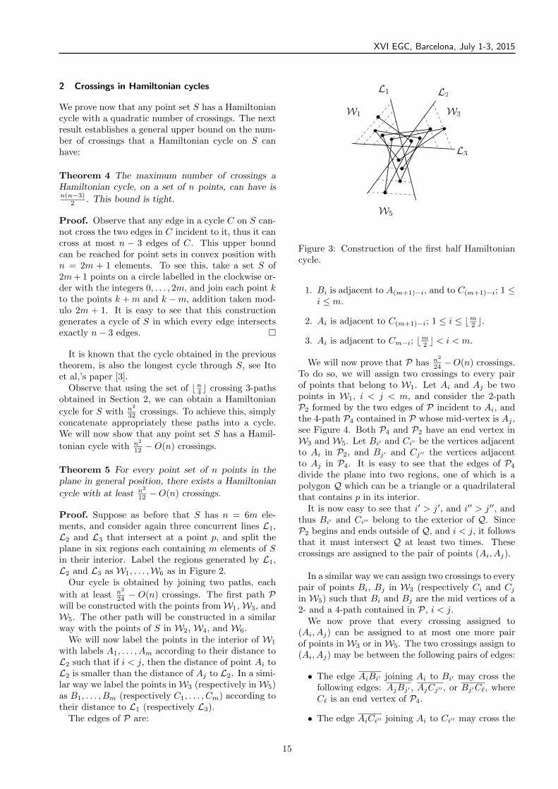
Computing the maximum overlap of a disk and a polygon with holesunder translation 57
Narcıs Coll, Marta Fort and J. Antoni Sellares
Session 5 - Thursday 14:40 – 16:00
The 2-center problem and ball operators in strictly convex normed planes 61
Pedro Martın, Horst Martini and Margarita Spirova
Combining surface and volume Reeb graphs for solid segmentation 65
Birgit Strodthoff and Bert Juettler
Minimum interference graph coloring and monochromatic edges 69
Javier Lorenzo Dıaz, David Orden, Ivan Marsa-Maestre, Jose Manuel Gimenez-Guzmanand Enrique de La Hoz
Grundy and pseudo-Grundy indices for geometric graphs 73
Dolores Lara, Christian Rubio-Montiel and Francisco Javier Zaragoza Martınez

Session 6 - Thursday 16:30 – 17:50
Orthogonal polygon illumination with rotating floodlights 77
Israel Aldana, David Flores, Jorge Urrutia, Carlos Velarde, Carmen Cedillo, JoelAguilar and Erick Solis
Almost empty monochromatic polygons in planar point sets 81
Alejandro C. Gonzalez-Martınez, Jorge Cravioto Lagos and Jorge Urrutia
The hamburger theorem 85
Jan Kyncl and Mikio Kano
On the number of anchored rectangle packings for a planar point set 89
Kevin Balas and Csaba Toth
Invited talk 4 - Friday 9:30 – 10:30
Ray configurations
Jorge Urrutia
Session 7 - Friday 11:00 – 13:00
Stabbing segments with rectilinear objects 93
Merce Claverol, Delia Garijo, Matias Korman, Carlos Seara and Rodrigo I. Silveira
Scribability problems for polytopes 97
Arnau Padrol and Hao Chen
Discrete Geometry on 3 Colored Point Sets in the Plane 101
Mikio Kano
Point sets in the plane as lengths of subsequences of permutations 104
Jose Luis Alvarez, Jorge Cravioto and Jorge Urrutia
On the disks with diameters the sides of a convex 5-gon 108
Clemens Huemer and Pablo Perez-Lantero
Stabbing circles for sets of segments in the plane 112
Merce Claverol, Elena Khramtcova, Evanthia Papadopoulou, Maria Saumell and CarlosSeara

XVI EGC, Barcelona, July 1-3, 2015
Non-crossing monotone paths and binary trees in edge-labeled completegeometric graphs
Frank Duque∗ †1, Ruy Fabila-Monroy ∗ ‡ 1, Carlos Hidalgo-Toscano ∗ §1, and Pablo Perez-Lantero ¶2
1Departamento de Matematicas, Cinvestav, D.F. Mexico, Mexico.2Escuela de Ingenierıa Civil en Informatica, Universidad de Valparaıso, Valparaiso, Chile.
Abstract
Let G be a geometric graph on n vertices whose edgesare labeled with distinct positive integers. A path inG is called monotone if its edge labels form a mono-tone sequence. A rooted tree in G is called monotoneif every path from the root to a leaf is monotone in-creasing or every path from the root to a leaf is mono-tone decreasing. Let α(G) be the maximum length ofa monotone non-crossing path in G. Let τ(G) be themaximum size of the monotone a non-crossing com-plete binary tree in G. In this paper, we give lowerand upper bounds on α(G) and τ(G), respectively.
Introduction
Let G = (V,E) be a graph. An edge labeling of G isan injective function N : E −→ Z. A monotone pathin G is a simple path P = v0, v1, . . . , vk in G such thatN(vivi+1) < N(vi+1vi+2) for all i = 0, 1, . . . , k − 2 orN(vivi+1) > N(vi+1vi+2) for all i = 0, 1, . . . , k − 2.The minimum over all edge labelings of the maxi-mum length of a monotone path is denoted by α(G).Chvatal and Komlos [3] raised the problem of esti-mating α(Kn). Currently, the best known bounds are12
(√4n− 3− 1
)≤ α(Kn) ≤
(12 + o(1)
)n. The lower
bound is due to Graham and Kleitman [4] and theupper bound to Calderbank and Chung [2]. The lat-ter authors conjectured that this is the right order ofmagnitude of α(Kn).
The parameter α(G) has been studied for specificfamilies of graphs. Bialostocki and Roditty showedthat α(G) ≥ 3 if and only if G contains as a sub-graph an odd cycle of length at least five or one of sixfixed graphs. Yuster [6] studied the parameter α∆,defined as the maximmum of α(G) over all graphswith maximum degree at most ∆, and proved that∆(1 − o(1)) ≤ α∆ ≤ ∆ + 1. Roditty, Shoham, and
∗Partially supported by Conacyt of Mexico, grant 153984.†Email: [email protected]‡Email: [email protected]§Email: [email protected]¶Partially supported by project Millennium Nucleus Infor-
mation and Coordination in Networks ICM/FIC RC130003(Chile). Email: [email protected]
Yuster [5] gave bounds for α(G) when G is a tree,a planar graph, or has bounded arboricity. Burger,Cockayne, and Mynhardt [1] gave upper bounds forα(G) when G is a complete or complete bipartitegraph, and gave exact values for some small graphs.
In this paper, we study α(G) and other parametersin the context of geometric graphs.
A geometric graph G is a graph whose vertices arepoints in the plane in general position and whoseedges are straight line segments joining these points.We say that G is a straight-line drawing of G if Gand G are isomorphic. Let α(G) be the minimumover all edge labelings of the maximum length of anon-crossing monotone path in G. Let α(G) be the
minimum of α(G) over all straight-line drawings G ofG.
A rooted binary tree in G is monotone increasing(decreasing) if all paths from the root to a leaf are
monotone increasing (decreasing). Let τ+(G) (τ−(G))be the minimum over all edge labelings of the maxi-mum size of a non-crossing monotone increasing (de-
creasing) rooted complete binary tree in G. Let τ+(G)
(τ−(G)) be the minimum of τ+(G) (τ−(G)) over all
straight-line drawings G of G. Let τ(G) be the min-imum over all edge labelings of the maximum size ofa non-crossing monotone rooted complete binary treein G and τ(G) the minimum of τ(G) over all straight-
line drawings G of G.
A convex geometric graph is a geometric graphwhose vertices are in convex position. A convexstraight-line drawing of a graph G is a convex geo-metric graph G that is isomorphic to G.
In this paper we prove that α(Kn) = Θ(n). For thecase of monotone trees, there is a gap between thelower and upper bounds. We prove that τ(Kn) =Ω(log log n) and τ(Kn) = O(
√n log n). As an in-
termediate result, if we are interested in boundingthe size of monotone increasing or monotone decreas-ing binary trees but not both, we prove the boundsτ+(Kn) = O(log n) and τ−(Kn) = O(log n).
1

XVI Spanish Meeting on Computational Geometry
1 Monotone non-crossing paths
Lemma 1 Let S be a set of points in convex po-sition and ` a straight line that splits S into twononempty parts U and V . The maximum length of anon-crossing polygonal chain whose vertices alternatebetween U and V and whose edges increase in slopeis two.
Proof. Assume that a polygonal P of length threewith the conditions of the statement exists. Let p, q, rdenote the first, second and third vertices of P , re-spectively, and assume that q ∈ U (the reasoning isanalogous if q ∈ V ). There exist three ways in whichthe first two edges of P can look like, as shown inFigure 1. In any case, the fourth vertex of P mustbe either in the convex wedge with apex q and ver-tices p and r in its boundary or across the supportingline of pq from r. In the first case, the convexity of Sis contradicted, in the second case a crossing in P isintroduced.
Figure 1: The fourth vertex of a polygonal with in-creasing slope must be in the shaded region.
Theorem 2 α(Kn) = Θ(log n).
Proof. Let Kn be a straight-line drawing of Kn andassume without loss of generality that no two verticesof Kn have the same x-coordinate. Let v1, . . . , vndenote the vertices of Kn in increasing order of x-coordinate, N an edge labeling of Kn, and H thecomplete 3-hypergraph with same vertex set as Kn.For 0 ≤ i < j < k ≤ n, color the edge (vi, vj , vk)of H blue if N(vivj) < N(vjvk), otherwise color itred. From Ramsey’s Theorem, there exists a com-plete monochromatic sub-hypergraph K of size m =Ω(log n) in H with vertices vi1 , vi2 , . . . , vim . Then,P = vi1 , vi2 , . . . , vim is a monotone path of length
Ω(log n) in Kn which has no crossings, as it is alsox-monotone.
Now, for the upper bound, let Kn be a convexstraight-line drawing of Kn. We define the follow-ing labeling N of Kn. Let ` be a vertical line thatpartitions the vertices of Kn into two sets U,W ofsize at most n/2 + 1. Label the edges between U and
W so that N(e) < N(e′) if and only if the slope of eis smaller than the slope of e′. Recursively label theedges of the subgraph Kn[U ] of Kn induced by U and
the edges of the subgraph Kn[W ] of Kn induced byW in such way that the edges between vertices in Uand V have larger labels than the ones in both Kn[U ]
and Kn[W ]. Now, let P be a monotone path of maxi-
mum length in Kn with respect to this edge labeling.By Lemma 1, there are at most two edges that go be-tween sets of the same level of recursion. Moreover,P cannot have edges both in Kn[U ] and Kn[W ], since
there would be a subpath with an edge in Kn[U ], an
edge between U and W and an edge in Kn[W ]; thispath cannot be monotone. Thus, the length T (n) ofP satisfies the recursion T (n) ≤ 2 + T (n/2), whichimplies T (n) = O(log n).
2 Monotone non-crossing complete binary trees
We can obtain a lower bound on τ(Kn) with the sameargument used to bound α(Kn).
Theorem 3 Let Kn be a convex straight-line draw-ing of Kn. Then, τ(Kn) = Ω(logn).
Proof. As before, let v1, v2, . . . , vn denote the ver-tices of Kn in increasing order of x-coordinate, Nan edge labeling of Kn, and H the complete 3-hypergraph with same vertex set as Kn. For 0 ≤i < j < k ≤ n, color the edge (vi, vj , vk) of H blueif N(vivj) < N(vjvk), otherwise color it red. FromRamsey’s theorem, there exists a complete monochro-matic sub-hypergraph K of size Ω(log n) in H. As-sume without loss of generality that at least half ofthe vertices of K lie on the lower convex hull of thevertices of Kn. Let vi1 , . . . , vim denote those verticesin counterclockwise order. Let m′ be the largest in-teger of the form 2h+1 − 1, for some integer h, suchthat m′ ≤ m. We embed a rooted complete binarytree T of size m′ and vertices vi1 , . . . , vim′ . Place theroot of T at vi1 , and inductively place its left andright subtrees at the vertices vi2 , . . . , vi(m′+1)/2
andvi(m′+1)/2+1
, . . . , vim′ with roots at vi2 and vi(m′+1)/2+1,
respectively (see Figure 2). Note that T is monotoneand has no crossings by construction.
Figure 2: A complete binary tree in H.
2

XVI EGC, Barcelona, July 1-3, 2015
Theorem 4 τ(Kn) = Ω(log log n).
Proof. Let Kn be a straight-line drawing of Kn. Bythe Erdos-Szekeres Theorem, there exists a set ofΩ(log n) vertices of Kn in convex position; the boundfollows from Theorem 3.
When we search for monotone paths, there is noneed to distinguish between monotone increasing andmonotone decreasing—traversing a monotone increas-ing path in opposite direction gives us a monotone de-creasing path of the same length and vice versa. Thisis not the case with complete binary trees. Theorem 3guarantees that we can find a monotone complete bi-nary tree of size Ω(log n), but it can be increasing ordecreasing.
An upper bound on τ(Kn) must take into accountboth monotone increasing and monotone decreasingcomplete binary trees. We start by bounding bothτ+(Kn) and τ−(Kn).
Theorem 5 τ+(Kn) = O(log n) and τ−(Kn) =O(log n).
Proof. Let Kn be a convex straight-line drawingof Kn. We give an edge labeling of Kn such thatτ+(Kn) = O(log n). The proof for τ−(Kn) = O(log n)is analogous. The supporting line of every edge e = uvof Kn partitions the vertices of Kn \ u, v into twosets, let Se be the smaller one. Construct a labelingN such that if N(e) < N(e′) then |Se| ≤ |Se′ |. Let Tbe a largest non-crossing increasing complete binarytree in Kn with root r with respect to N .
Let L and R be the convex hulls of the left andright subtrees of T , respectively. We claim that Land R are disjoint. Suppose this is not the case. Letl, v1, . . . , vs, r
′ be the the vertices of L∪R sorted radi-ally around r starting with the root of the left subtreeand ending with the root of the right subtree. Theremust be a vertex of R followed by a vertex of L inthis order, otherwise L and R are disjoint; let vi bethe first such vertex of R in this order and l′ = vi+1.In the path that joins vi with r′ in T , there exists atleast one edge vjvk with j ≤ i < k. The vertices l andl′ lie on different sides of the supporting line of vjvk,so the path that joins them in T must cross vjvk. Thisis a contradiction, since T is non-crossing.
Let ` be a line through r that separates L and R.The line ` partitions the vertices of Kn \ r into twoparts, one with less than n/2 vertices. Let T ′ be thesubtree of T contained in this part.
Let h′ be the height of T ′. For 0 ≤ h ≤ h′, letTh,s be the set of subtrees of T ′ of height h such thatthe edge that joins them with their parent has labellarger than s. Let T (h, s) be the minimum of thelargest label of each tree in Th,s.
Note that for every vertex v of T ′ with children uand w either the subtree Tu rooted at u is contained
in Svw or the subtree Tw rooted at w is contained inSvu. Assume without loss of generality that the firstcase happens. This implies that every edge of Tu iscontained in Svw. Thus, the label of every edge of Tuis smaller than the label of vw. Therefore, T (h, s) ≥T (h − 1, T (h, s)). It can be shown by induction that
T (h, s) = Ω(s22h
). Thus, there is a label in T ′ of size
at least Ω(22h
). This implies that h′ = O(log logn).Therefore, T has at most O(log n) vertices.
The edge labeling used in the proof of Theorem 5forbids large monotone increasing binary trees, but itis possible to find a monotone decreasing binary treeof linear size. Theorem 6 gives an edge labeling thatforbids both increasing and decreasing large binarytrees.
Theorem 6 τ(Kn) = O(√n log n).
Proof. Let Kn be a convex straight-line drawing ofKn. Let v1, . . . , vn denote the vertices of Kn in coun-
terclockwise order. Let m =⌈√
n/ log n⌉
and par-
tition the vertices into groups S1, S2, . . . , Sm of con-secutive vertices such that each one has size at most⌈√
n log n⌉. Label the edges with endpoints within
Si with the same edge labeling as in Theorem 5 suchthat the largest non-crossing decreasing complete bi-nary tree contained in Si has size at most O(log n).We refer to these edges as red edges. We refer tothe edges with endpoints in different groups as blueedges. Label the blue edges by increasing slope. Fur-thermore, choose the labels in such a way that everyblue edge has larger label than every red edge.
Let T be a monotone decreasing complete binarytree with respect to this labeling. Note that T con-sists of a possibly empty blue binary tree Tb and a for-est of red complete binary trees such that the rootsof the red trees are leaves of Tb (Figure 3). Notethat since Tb is non-crossing, the subgraph of Tb in-duced by blue edges between two different groups Si
and Sj has at most two connected components. ByLemma 1, these components are trees of height atmost three. Therefore the number of edges betweentwo different groups Si and Sj is at most a constant.Let u1, . . . , um be vertices on a circle ordered coun-terclockwise. Add an edge between ui and uj if andonly if there is an edge in Tb between Si and Sj .Since Tb is non-crossing, the resulting graph is alsonon-crossing; it has O(
√n/ log n) edges. Therefore,
Tb has at most O(√n/ log n) edges. Since there are
O(√n/ log n) leaves in Tb, there are O(
√n/ log n) red
trees, each with size at most O(log n). Thus, T hassize O(
√n log n).
Now consider a monotone increasing complete bi-nary tree T with respect to this labeling. Note that Tconsists of a possibly empty red binary tree Tr and aforest of blue complete binary trees such that the roots
3

XVI Spanish Meeting on Computational Geometry
Figure 3: A monotone deccreasing complete binarytree with respect to the ordering of Theorem 6.
of the red trees are leaves of Tr (Figure 4). The treeTr is contained in some Sr, so it has size O(
√n log n).
Identify all the roots of the blue trees with a vertexof Sr, this produces a non crossing blue tree. Thereare at most O(
√n log n) blue edges with an endpoint
in Sr. We can bound the number of remaining blueedges as before by O(
√n/ log n). Therefore, T has
size O(√n log n).
Figure 4: A monotone inscreasing complete binarytree with respect to the ordering of Theorem 6.
References
[1] A. P. Burger, E. J. Cockayne, and C. M. Mynhardt.Altitude of small complete and complete bipartitegraphs. Australas. J. Combin., 31:167–177, 2005.
[2] A. R. Calderbank, F. R. K. Chung, and D. G. Sturte-vant. Increasing sequences with nonzero block sumsand increasing paths in edge-ordered graphs. DiscreteMath., 50(1):15–28, 1984.
[3] V. Chvatal and J. Komlos. Some combinatorial the-orems on monotonicity. Canad. Math. Bull., 14:151–157, 1971.
[4] R. L. Graham and D. J. Kleitman. Increasing paths inedge ordered graphs. Period. Math. Hungar., 3:141–148, 1973. Collection of articles dedicated to the mem-ory of Alfred Renyi, II.
[5] Yehuda Roditty, Barack Shoham, and Raphael Yuster.Monotone paths in edge-ordered sparse graphs. Dis-crete Math., 226(1-3):411–417, 2001.
[6] Raphael Yuster. Large monotone paths in graphswith bounded degree. Graphs Combin., 17(3):579–587,2001.
Por que no sale esto ...Por que no sale esto ...
4

XVI EGC, Barcelona, July 1-3, 2015
On Hamiltonian alternating cycles and paths
Merce Claverol∗1, Alfredo Garcıa†2, Delia Garijo‡3, Carlos Seara∗4, and Javier Tejel†2
1Departament de Matematica Aplicada IV, Universitat Politecnica de Catalunya, Spain.2Departamento de Metodos Estadısticos, IUMA, Universidad de Zaragoza, Spain.
3Departamento de Matematica Aplicada I, Universidad de Sevilla, Spain.4Departament de Matematica Aplicada II, Universitat Politecnica de Catalunya, Spain.
Abstract
A natural relaxation for problems that have no solu-tion for plane geometric graphs is to allow the geomet-ric graphs to be 1-plane, that is, there can be at mostone crossing per edge. In this work, we study this re-laxation for Hamiltonian alternating cycles and paths.Thus, it is well-known that one cannot always drawa plane Hamiltonian alternating cycle, even on a bi-colored point set in convex position, whilst we provethat allowing the cycle to be 1-plane, it can alwaysbe found, on a point set in general position, in O(n2)time and space. We also restrict ourselves to bicoloredpoint sets in convex position obtaining a remarkablevariety of results. Among them, we show that everyHamiltonian alternating cycle with minimum numberof crossings is 1-plane, and we compute Hamiltonianalternating cycles and paths with minimum numberof crossings in, respectively, O(n) and O(n2) time andspace.
Introduction
Let R and B be two disjoint sets of red and bluepoints in the plane, respectively, such that S = R∪Bis in general position (i.e, no three points lie on thesame line). A Hamiltonian alternating path on S isa path passing through every point of S such thatits edges are straight-line segments, and any two con-secutive vertices have distinct colors. A Hamiltonianalternating cycle is analogously defined. Thus, unlessotherwise stated, |B| = n and n ≤ |R| ≤ n + 1.
When there are no crossings, such paths and cyclesare said to be plane, and they are 1-plane if everyedge is allowed to have at most one crossing. Observethat the terms plane graph and 1-plane graph referto a geometric object, while to be planar or 1-planar
∗Emails: [email protected], [email protected]. Re-search supported by proyects Gen. Cat. DGR 2014SGR46 andMINECO MTM2012-30951.†Emails: [email protected], [email protected]. Research sup-
ported by Gobierno de Aragon under grant E58 (ESF) andproject MINECO MTM2012-30951.‡Email: [email protected]. Research supported by proyect
2011/FQM-164.
r
bp3 p4 p6
p1 p2 p5
Figure 1: Left: A 1-PHAC. Right: A configurationthat does not admit a 1-PHAP with endpoints r, b.
are properties of the underlying abstract graph. Forshort, we shall write 1-PHAC and 1-PHAP to refer toa 1-plane Hamiltonian alternating cycle and a 1-planeHamiltonian alternating path, respectively. Figure 1(left) illustrates a 1-PHAC1.
From the fact that one cannot always find a Hamil-tonian alternating path, even if S is in convex po-sition, arose the interest to study such geometricgraphs. According to Pach [8], the first study is dueto Erdos [5] who proposed in 1989 to determine orestimate the largest number `(n) such that, for everyset of n red and n blue points on a circle (i.e., in con-vex position), there exists a non-crossing alternatingpath consisting of `(n) vertices. Erdos conjecturedthat `(n) = 3
2n + 2 + o(n), but one can find pointconfigurations for which `(n) < 4
3n + o(n) [1, 8]. Thebest bounds up to date for `(n) are due to Kyncl,Pach and Toth [8], and valid for bicolored point setsin general position. However, the conjecture that|`(n) − 4
3n| = o(n) remains open, even for points inconvex position.
On the other hand, Akiyama and Urrutia [2] gavean O(n2) time algorithm for computing a plane alter-nating path visiting the maximum possible number ofpoints, provided that the point set is in convex po-sition and the endpoints of the path are previouslyfixed. Moreover, Kaneko, Kano and Yoshimoto [7]proved that there always exists a Hamiltonian alter-nating cycle on a bicolored point set in general posi-tion with at most n − 1 crossings. See [6] for morereferences on bicolored point sets.
Due to the impossibility of achieving the plane char-
1In the figures in this work, red points are illustrated as solidred points, and blue points are depicted as hollow blue points.
5

XVI Spanish Meeting on Computational Geometry
acter, and as a natural relaxation on the constraint,Hurtado et al. [3] proposed to study 1-plane geometricgraphs in general, emphasizing on 1-plane Hamilto-nian alternating cycles and paths. They proved thatone can always draw a 1-PHAC on a point set in con-vex position, and also on a double chain. They alsoconjectured the existence of a 1-PHAP for point setsin general position. Our main result in Section 1 (The-orem 3) settles in the affirmative this conjecture, andis even stronger, since we prove that not only a pathbut a 1-PHAC can always be obtained on a point setin general position, also upper-bounding the numberof crossings. Our approach lets us also show that sucha cycle can be computed in O(n2) time and space.
Section 2 concerns Hamiltonian alternating cyclesand paths on bicolored point sets in convex position.Theorem 5 provides a lower bound for the numberof crossings, and states that only some cycles thatare 1-plane attain the bound. We also character-ize the point configurations that do not admit a 1-PHAP with given endpoints, and for the remainingwe show every optimum Hamiltonian alternating path(i.e., with minimum number of crossings) is 1-plane.We conclude in Theorem 9 analyzing the complexi-ties of computing optimum Hamiltonian alternatingpaths and cycles. These complexities are O(n) (forcycles and paths with consecutive endpoints of S) andO(n2) (for all paths).
We want to point out that most proofs in this workinvolve a number of technical results and long caseanalysis. Thus, due to the space limitation, they areomitted, although we give some brief explanations.
1 General position
We first consider the problem of drawing a 1-PHAC ona set S = R∪B in general position with n = |R| = |B|.Our approach follows the technique of Kaneko, Kanoand Yoshimoto [7] to construct a Hamiltonian alter-nating cycle with at most n − 1 crossings, but withimportant differences. Indeed, the main tool of theirtechnique is the fact that there always exists a Hamil-tonian alternating path with at most n − 1 crossingsconnecting any red point to any blue point, both lo-cated on the boundary of CH(S)2. Then, they usean effective way of splitting S into adequate subsetsin which, by induction, one can draw such paths sothat they can be connected giving rise to the desiredcycle. Our main obstacle is that when the path is al-lowed to be 1-plane, red and blue arbitrary points onthe boundary of CH(S) cannot always be connected;see Figure 1 (right). This fact is captured in Lemma2, which says that one can fix the endpoints of a 1-PHAP in all cases except for the special configurationsof Definition 1.
2As usual, the convex hull of a point set X ⊆ S is denotedby CH(X).
pi
pi+1
r
r2r1
S1
S2
p′i′p′i′+1
r
r2r1
S1
S2
Figure 2: A counterclockwise partition (left) and aclockwise partition (right) of S around r.
On the other hand, our approach makes possiblebounding the number of crossings, not only by n− 1but using the number of runs of S. A run of S is amaximal set of consecutive points of the same coloron the boundary of CH(S), which can be red or bluedepending on the color of the points. We write r(X)and b(X) to denote the number of red and blue runsof S, respectively; observe that r(S) = b(S) wheneverthe boundary of CH(S) contains points of both colors.
The following lemma, which is an adaptation ofLemma 1 of [7], gives the method to split S into theabove-mentioned adequate subsets; see also Figure 2.For the sake of brevity, we only state the result for|R| = |B| = n ≥ 1 but a similar result holds for|R| = |B|+ 1 = n + 1 ≥ 2.
Lemma 1 Let S = R∪B be in general position, andlet r be an arbitrary red point of S. Suppose that|R| = |B| = n ≥ 1, p1, . . . , p2n−1 is the counter-clockwise radial order of the points of S \ r aroundr, and pi+1 is the first point in that sequence such that|r, p1, . . . , pi+1 ∩R| = |r, p1, . . . , pi+1 ∩B|. Then,(a) pi+1 = p1 if p1 is blue, (b) pi and pi+1 both existand are blue whenever p1 is red. In this last case, wesay that S1 = p1, . . . , pi and S2 = pi+1, . . . , p2n−1form a counterclockwise partition of S \r around r.
If we explore the points of S\r in clockwise order,we obtain the clockwise partition of S \ r around r,where there are points p′i′ , p
′i′+1 playing the role of pi,
pi+1; see Figure 2 (right).
Definition 1 Let S = R ∪ B such that r ∈ R andb ∈ B are on the boundary of CH(S). The triple(S, r, b) is a special configuration if:
(i) The two neighbors of r on the boundary ofCH(S) are red, and those of b are blue.
(ii) In the clockwise and counterclockwise partitionsof S around r, pi+1 = p′i′+1 = b.
(iii) In the clockwise and counterclockwise partitionsof S around b, pi+1 = p′i′+1 = r.
Otherwise, the configuration (S, r, b) is non-special.
6

XVI EGC, Barcelona, July 1-3, 2015
Figure 1 (right) illustrates a special configuration(S, r, b). In the counterclockwise partition of S aroundr, S1 = p1, p2, p3, p4 and so pi+1 = b; for theclockwise partition we have S1 = p5, p6, and againp′i′+1 = b. The same happens for the clockwise andcounterclockwise partitions of S around b: points pi+1
and p′i′+1 coincide with r.As it was explained before, the following lemma is
the main tool to reach Theorem 3 below. Its proofshows simultaneously both statements by inductionon |S|, using the partitions of Lemma 1 and perform-ing a case analysis.
Lemma 2 Let S = R ∪B, and let r be an arbitraryred point on the boundary of CH(S). Then, the fol-lowing statements hold.
(i) If |R| = |B| = n ≥ 1 and there is a blue point bon the boundary of CH(S) such that the config-uration (S, r, b) is non-special, then there existsa 1-PHAP on S with endpoints r, b and at mostn− r(S) crossings.
(ii) If |R| = |B| + 1 = n + 1 ≥ 2 and there is ared point r′ on the boundary of CH(S) differentfrom r, then there exists a 1-PHAP on S withendpoints r, r′ and at most n− b(S) crossings.
By using the Ham-sandwich theorem and Lemma 2,we can prove our main result in this section.
Theorem 3 For given S = R ∪ B with |B| = |R| =n ≥ 2, there exists a 1-plane Hamiltonian alternatingcycle on S with at most n−maxr(S), b(S) crossings.
The bound of n−maxr(S), b(S) for the numberof crossings is tight: a point set S consisting of 2npoints in convex position, n consecutive red pointsand n consecutive blue points attains the bound [7].However, there are configurations of points for whichthis bound is far to be tight: if the n red points areon the boundary of CH(S) and the n blue points areinside CH(S), then there is a Hamiltonian alternatingcycle on S with no crossings [4], and the bound ofTheorem 3 would be n− 1.
Lemma 2 and Theorem 3 let us compute a 1-PHAC,not necessarily minimizing the number of crossings, inO(n2) time and space.
Corollary 4 For given S = R ∪ B with |B| = |R| =n ≥ 2, a 1-plane Hamiltonian alternating cycle on Scan be computed in O(n2) time and space.
2 Convex position
We now turn to a natural restriction of our study thatis to consider point sets S in convex position. We firstobtain that, in this case, the bound of Theorem 3 isa lower bound for the number of crossings of every
Hamiltonian alternating cycle on S, and moreover,only cycles that are 1-plane attain the bound.
Theorem 5 Let S = R ∪ B be in convex positionwith |R| = |B| = n ≥ 2. Then,
(i) Every Hamiltonian alternating cycle on S has atleast n− r(S) crossings.
(ii) A Hamiltonian alternating cycle on S with n −r(S) crossings is 1-plane.
The converse of statement (ii) in the preceding the-orem is not true, i.e., it is possible to construct a1-PHAC on a set S with more than n − r(S) cross-ings. For instance, if S consists of points alternatingin color then r(S) = n, and obviously one can draw a1-PHAC without crossings, but also a 1-PHAC withdn2 e or dn2 e+ 1 crossings (depending on the parity ofn). Moreover, using the same point configuration, itis not difficult to check that the number of different1-plane Hamiltonian alternating cycles on a point setcan be exponential.
Regarding paths, recall that by Lemma 2, one canalways draw a 1-PHAP with given endpoints, pro-vided that the point configuration is non-special (incase that those endpoints are of distinct colors). Thefollowing theorem states that for point sets in convexposition, special configurations are the unique config-urations of points that do not admit such a path.
Theorem 6 Let S = R ∪ B be in convex positionwith |R| = |B| = n ≥ 1. Given r ∈ R and b ∈ B,there exists a 1-plane Hamiltonian alternating path onS with endpoints r, b if and only if the configuration(S, r, b) is non-special.
On the other hand, when the configuration is non-special, one may wonder whether being optimum im-plies being 1-plane. This is the analogous problemas that considered in Theorem 5(ii) for cycles, butthere is a fundamental difference: the path has fixedendpoints, which have the same color or not.
Theorem 7 Let S = R ∪ B be in convex positionwith |R| = |B| ≥ 1 or |R| = |B| + 1 ≥ 2, and letps, pt ∈ S such that the configuration (S, ps, pt) isnon-special if ps, pt have distinct colors. Then, ev-ery optimum Hamiltonian alternating path on S withendpoints ps, pt is 1-plane.
The preceding theorem is proved by assuming thatthere exists such an optimum path, say Opt, and thatan edge is crossed by two other edges. Depending onthe positions of the endpoints of those edges and theircolors, we distinguish a number of cases. A contra-diction (with Opt being optimum) is reached in eachcase, by using a technical lemma that gives informa-tion about the order in which Opt must visit some
7

XVI Spanish Meeting on Computational Geometry
subsets of points, and a property based on the quad-rangular property. All the arguments of this proof,except for those in one case, can be used for specialconfigurations to show that no edge of Opt can becrossed twice. In that specific case, we obtain thatOpt has only one edge that is crossed twice. This iscontained in the following corollary.
Corollary 8 Let (S, r, b) be a special configurationfor a point set S = R ∪ B in convex position with|R| = |B| = n ≥ 1. Then, every Hamiltonian al-ternating path on S with endpoints r, b has at leastn − r(S) crossings. Moreover, an optimum Hamilto-nian alternating path on S with endpoints r, b can becomputed in O(n) time, has n − r(S) crossings, andall its edges are crossed at most once, except for oneof them that is crossed twice.
Finally, we analyze the complexities of computingoptimum Hamiltonian alternating paths and cycles onS in convex position. Recall that, by Corollary 4,when S is in general position, a 1-PHAC (not neces-sarily optimum) can be computed in O(n2) time andspace.
Theorem 9 For given S = R∪B in convex position,the following statements hold.
(i) If |R| = |B| = n ≥ 2, then an optimum Hamilto-nian alternating cycle on S can be computed inO(n) time and space.
(ii) Let ps, pt ∈ S with either distinct colors if |R| =|B| ≥ 1 or the same color if |R| = |B| + 1 ≥ 2.Then, an optimum Hamiltonian alternating pathon S with endpoints ps, pt can be computed inO(n2) time and space. Further, such a path canbe computed in O(n) time and space when ps, ptare consecutive points of S.
Moreover, in all cases, the optimum is 1-plane.
The proof of statement (i) in the preceding theo-rem is based on a linear procedure that computes,for every point pi of one color, the first clockwisepoint pJ(i) of the other color such that, between them,there are the same number of red and blue points.This lets us show that the process developed in theproof of Lemma 2 (here omitted) can be done in lin-ear time. A similar argument applies to prove state-ment (ii) for consecutive endpoints of the path. Fornon-consecutive endpoints ps, pt (also statement (ii)),we design an O(n2) time and space dynamic program-ming algorithm which uses as a main tool that it is al-ways possible to find an optimum 1-PHAP with thoseendpoints that contains either an optimum sub-pathfrom ps to pJ(s), or an optimum sub-path from ps topJ′(s) (where this point is obtained as pJ(i) but per-forming the same procedure counterclockwise).
3 Conclusion
We conclude by formulating some problems, relatedto those here considered, that remain open.
• For point sets S in general position:
Problem 1. Characterize the special configurations(S, r, b) that do admit a 1-PHAP.Problem 2. Among all optimum Hamiltonian alter-nating cycles on S, determine whether there is at leastone that is 1-plane.Problem 3. Decide whether it is possible to computein polynomial time an optimum 1-PHAC on S.
• For point sets S in convex position:
Problem 4. Prove that the number of 1-plane Hamil-tonian alternating cycles on S is exponential in r(S).
Acknowledgements
The authors want to dedicate this work in memorialof Prof. Ferran Hurtado. More particularly, Delia,Merce and Carlos are specially much grateful for shar-ing with Ferran the pleasure of arising together thefirst ideas and formalizations of the problem.
References
[1] M. Abellanas, A. Garcıa, F. Hurtado and J. Tejel,Caminos alternantes, in: Actas X Encuentros de Ge-ometrıa Computacional (in Spanish), 2003, 7–12.
[2] J. Akiyama and J. Urrutia, Simple alternating pathproblem, Discr. Math. 84 (1990), 101–103.
[3] M. Claverol, D. Garijo, F. Hurtado, D. Lara and C.Seara, The alternating path problem revisited, in:Proc. XV Spanish Meeting on Comp. Geom., 2013,115–118.
[4] A. Garcıa and J. Tejel, Dividiendo una nube de pun-tos en regiones convexas, in: Actas VI Encuentros deGeometrıa Computacional, 1995, 169–174.
[5] Paul Erdos, Personal communication to J. Pach(see [8]).
[6] A. Kaneko and M. Kano, Discrete geometry on redand blue points in the plane - a survey, in: Discreteand Computational Geometry, The Goodman-PollackFestschrift; edited by B. Aronov et al., Springer, 2003,551–570.
[7] A. Kaneko, M. Kano and Y. Yoshimoto, AlternatingHamiltonian cycles with minimum number of cross-ings in the plane, Int. J. Comput. Geom. Appl. 10(2000), 73–78.
[8] J. Kyncl, J. Pach and G. Toth, Long alternatingpaths in bicolored point sets, in: Graph Drawing2004 (J. Pach, ed.), Lecture Notes in Computer Sci-ence 3383, 2004, 340–348. Also in Discr. Math. 308(2008), 4315–4322.
8

XVI EGC, Barcelona, July 1-3, 2015
The bipartite traveling salesman problem for convex point sets
Alfredo Garcıa∗1 and Javier Tejel∗1
1Departamento de Metodos Estadısticos, IUMA, Universidad de Zaragoza, Spain
Abstract
Given a bicolored convex point set S = R ∪ B, with|R| = |B| = n, we provide an O(n6) algorithm tofind the shortest Hamiltonian cycle C, visiting alter-natively the points of R and B. The algorithm isbased on characterizing the possible order in whichthe points of S can appear in C. This algorithm canalso be used to construct the shortest Hamiltoniancycle C such that C visits alternatively the bicoloredvertices of a simple polygon P and is inside P .
Introduction
In the bipartite traveling salesman problem (BTSP),one is given a partition of a prescribed set of citiesinto two classes R and B, with |R| = |B|, and onewishes to find the shortest route such that the citiesin R and B alternate along the route. At first glance,dividing the cities into two classes seems to be a bitartificial, but the BTSP appears in a natural way as aparticular case for different types of problems, mainlyin typical industrial settings where pick and place orgrasp and delivery robots are employed with some ma-terial handling tasks. See for example [10].
It is well-known that the BTSP and the EuclideanBTSP (the cities are assumed to be points on theplane) are NP-hard, so there is no polynomial algo-rithm to solve them unless P = NP . Researchershave been focused on designing good approximationalgorithms or solving particular cases. We refer thereader to [2, 4, 7, 9, 10] and the references thereinfor different approximation algorithms along with ex-perimental results. When the cities are on a line ora tree, the BTSP can be solved in O(n) and O(n2)time, respectively [12]. In [6], the authors solve an-other particular case. They give an O(n4) algorithmto decide whether there is a renumbering of the ncities such that the elements of the resulting distancematrix satisfy a set of inequalities. If this is the case,the shortest tour can be obtained directly from thisrenumbering. This set of inequalities is in fact a re-laxation of the Monge property: cij + clm ≤ cim + clj ,for i < l and j < m.
∗Emails: [email protected], [email protected]. Research sup-ported by Gobierno de Aragon under grant E58 (ESF) andproject MINECO MTM2012-30951.
In this paper, we assume that the cities are bicol-ored points on the plane and we focus on studying theparticular case in which the points are in convex posi-tion. Under this assumption, Section 2 is devoted tocharacterizing the order of the points in any optimumtour for the BTSP, using a technical lemma proved inSection 1. This characterization allows us to designan O(n6) algorithm, described in Section 3, to solvethe BTSP for the convex case. Finally, in Section 4,we extend the characterization and the algorithm tofind the optimum tour inside a simple polygon, whichvisits alternatively the bicolored vertices of the poly-gon.
1 A technical lemma
Given a point set S on the plane, a polygonalpath P is a curve specified by a sequence of pointsp1, p2, . . . , pk+1 called its vertices, where k ≥ 1 andpi 6= pj for all i, j. The curve itself consists of theline segments e1 = p1p2, e2 = p2p3, . . . , ek = pkpk+1
connecting the consecutive vertices. We consider P asan oriented path, so P begins at point p1, finishes atpoint pk+1 and all the edges ei = pipi+1 are orientedfrom pi to pi+1. A polygonal path is called simple ifonly consecutive segments intersect and only at theirendpoints.
The following lemma allows us to associate a simplepolygonal path with every non-simple polygonal path.
Lemma 1 Let P be a polygonal path connectingp1 to pk+1, consisting of consecutive segments e1 =p1p2, e2 = p2p3, . . . , ek = pkpk+1. Then, there ex-ists a simple polygonal path P ′ connecting p1 topk+1 consisting of a sequence of consecutive segmentse′i1 , e
′i2, . . . , e′ih such that every segment e′ij is con-
tained in segment eij and 1 = i1 < i2 < . . . < ih = k.
Figure 1 shows an example of the lemma. The thickersegments correspond to P ′. Observe that if segmente′i appears before segment e′j in P ′, then segment eiappears before segment ej in path P = p1, . . . , p17.
Proof. The proof is by induction on k. If k = 1,P consists of segment e1 = p1p2, so P is simpleand coincides with P ′. Suppose the lemma holdsfor any polygonal path consisting of ≤ k − 1 seg-ments. Hence, by induction, the polygonal path
9

XVI Spanish Meeting on Computational Geometry
p1
p2p3
p4 p5
p6p7
p8
p9
p10p11
p12
p13
p14
p17e′1
e′5e′10
e′11
e′13
p16
p15
p′
e′14
e′16
P
P ′
Figure 1: The simple polygonal path P ′ obtained fromthe non-simple polygonal path P .
Pk−1 = e1, . . . , ek−1 connecting p1 to pk containsa simple polygonal path P ′k−1 consisting of segmentse′i1 , . . . , e
′ih
, with i1 = 1 < i2 < . . . < ih = k − 1, ande′ij ⊆ eij for j = 1, . . . , h. Let p′ be the first point
of P ′k−1 that is also a point of segment ek = pkpk+1.That point exists because at least pk is a commonpoint for both P ′k−1 and ek. Then, by construction,the subpath P ′′ of P ′k−1 consisting of the points fromp1 to p′ has p′ as the only common point with seg-ment e′k = p′pk+1. Therefore, the path P ′ obtainedby gluing segment e′k = p′pk+1 to P ′′ satisfies all thesought properties.
2 Points in convex position
Let S be a point set in convex position and let CH(S)be the convex hull of S. We suppose that the points ofS appear clockwise in the cyclic order p1, p2, . . . , p2non the boundary of CH(S). A Hamiltonian cycle C onS is given by a cyclic permutation (pi1 , pi2 , . . . , pi2n)of the points of S, where C is assumed to be a directedcycle, consisting of the directed segments (or edges)pi1pi2 , pi2pi3 . . . , pi2n−1
pi2n , pi2npi1 . The length of C is
the amount l(C) =∑2n
j=1 d(pij , pij+1), where d(pi, pj)is the Euclidean distance from pi to pj , identifyingpi2n+1
with pi1 . Given five points pi1 , pi2 , pi3 , pi4 , pi5in clockwise order on the boundary of CH(S) and aHamiltonian cycle C on S, we say the five points forma five points star if they appear in C in the orderpi1 , . . . , pi3 , . . . , pi5 , . . . , pi2 , . . . , pi4 , . . . or in the orderpi1 , . . . , pi4 , . . . , pi2 , . . . , pi5 , . . . , pi3 , . . ..
We assume that the points of S are partitioned intotwo classes, R and B, such that |R| = |B| = n. R isthe set of red points and B is the set of blue points.A cycle (path) is alternating if any two consecutivevertices have distinct colors. The following theoremshows that any optimum Hamiltonian alternating cy-cle cannot contain a five points star. Figure 2 showsthe shortest Hamiltonian alternating cycle C for that
p1
p2p3 p4
p5p6
p7p8
p9p10
p11
p12
Figure 2: The shortest Hamiltonian alternating cyclefor this convex point set.
convex point set, where red points are illustrated assolid red points and blue points as hollow blue points.Observe that C does not contain a five points star.The proof of the theorem is mainly based on Lemma1 and the well-known quadrangular property: Givena geometric graph G, if edge e = pq crosses edgee′ = p′q′, then the length of the geometric graphG′ obtained by replacing edges e, e′ by edges pp′, qq′
(or replacing them by edges pq′, qp′ ) is less than thelength of graph G. Of course, if graph G′′ is obtainedfrom G by applying this transformation several times,G′′ is shorter than G. Using the quadrangular prop-erty, it is not difficult to check the next two propertiesfor the shortest Hamiltonian alternating cycle, C, onS (see [3] for details).
P1 If the directed edge ei = piqi crosses the directededge ej = pjqj , then points pi, pj must have thesame color (and therefore qi, qj have the othercolor)
P2 C cannot contain three edges ei = piqi, ej =pjqj , ek = pkqk crossing each other.
Theorem 2 Let S = R ∪B be a point set in convexposition, where |R| = |B| = n. If C is the shortestHamiltonian alternating cycle on S, then C cannotcontain a five points star.
Proof. Assuming that five points pi1 , pi2 , pi3 , pi4 ,pi5 , clockwise on the boundary of CH(S), ap-pear in C in the cyclic order pi1 , . . . , pi3 , . . . , pi5 , . . . ,pi2 , . . . , pi4 , . . ., a contradiction is reached. The samereasoning can be applied to the symmetric orderpi1 , . . . , pi4 , . . . , pi2 , . . . , pi5 , . . . , pi3 , . . ..
Let P1, P3, P5, P2, P4 be the polygonal paths con-sisting of the edges of C connecting pi1 to pi3 , pi3 topi5 , pi5 to pi2 , pi2 to pi4 and pi4 to pi1 respectively. LetP ′1, P
′3, P
′5, P
′2, P
′4 be the corresponding simple polyg-
onal paths obtained by applying Lemma 1 to thosepaths. By construction, the polygonal path P ′5 mustbe crossed by P ′1 and P ′4. Among all the intersectionpoints between P ′4 and P ′5, let q4 be the first one onP ′4, and among all the intersection points between P ′1and P ′5, let q1 be the last one on P ′1. Note that q4must be a crossing point between an edge e′5 = p′5q
′5
10

XVI EGC, Barcelona, July 1-3, 2015
pi5
pi3pi4
pi1
pi2
p′5q′5
p′4
q′4p′1
q′1
q4 q1
pi5
pi3pi4
pi1
pi2p′5
q′5
p′4
q′4p′1
q′1
q4
q1p′′5
q′′5
pi5
pi3pi4
pi1
pi2
p′5q′5
p′4
q′4 p′1
q′1
q4 q1
pi5
pi3pi4
pi1
pi2
p′5 q′5
p′4
q′4 p′1
q′1
q4
q1p′′5
q′′5
Figure 3: Point q4 appears before point q1 in P5.
of P5 and an edge e′4 = p′4q′4 of P4, and q1 must be a
crossing point between an edge e′′5 = p′′5q′′5 of P5 and
an edge e′1 = p′1q′1 of P1. We distinguish two cases
depending on the order of q1 and q4 on P5.
Case 1: q4 appears before q1 in P5
In this case, e′′5 must appear after e′5 in P5 or bothedges coincide. Suppose first that both edges coincide,so q4 is placed before q1 on e′5 = e′′5 . See top part ofFigure 3. As triple crossings are forbidden by propertyP2, then necessarily edges e′1 and e′4 do not cross eachother. Moreover, since q4 is the first crossing pointbetween P ′4 and P ′5 on P ′4 and q1 is the last crossingpoint between P ′1 and P ′5 on P ′1 , p′4 must be to theright of e′5 and p′1 must be to the left of e′5. Observethat, by property P1, p′1 6= q′4, p
′4 6= q′1, p′1, p
′4, p′5 have
the same color and q′1, q′4, q′5 the other color. By ap-
plying the quadrangular property twice, first replac-ing edges e′5, e
′4 by edges s5 = p′5q
′4 and s4 = p′4q
′5
and then replacing edges e′1, s4 by edges s1 = p′1q′5
and s′4 = p′4q′1, we obtain a shorter cycle. Specifi-
cally, if we denote by P1a, P1b, P4a, P4b and P5a, P5b
the three couples of paths obtained from P1, P3, P5
when edges e′1, e′4, e′5 are removed, then cycle C
is P1a, e′1, P1b, P3, P5a, e
′5, P5b, P2, P4a, e
′4, P4b and the
cycle C ′ = P1a, s1, P5b, P2, P4a, s′4, P1b, P3, P5a, s5, P4b
would be shorter than C.
Suppose now that e′5 is different from e′′5 . Again,by applying the quadrangular property twice, replac-ing edges e′5, e
′4 by edges s5 = p′5q
′4, s4 = p′4q
′5, and
edges e′1, e′′5 by edges s1 = p′1q
′′5 , s′′5 = p′′5q
′1 we obtain
a shorter cycle (bottom part of Figure 3).
Case 2: q1 appears before q4 in P5
Due to space limitations, we do not explain this casein detail. The reasoning is based again on applyingthe quadrangular property twice. The main differencein relation to Case 1 is that now paths P ′4 and P ′1 mustcross at a point q′, placed in the region bounded bypath P ′5 and the part of the boundary of CH(S) frompi2 to pi5 , and the edges producing this crossing pointmust be used to apply the quadrangular property.
3 Algorithm
Cyclic permutations of the set 1, 2, . . . , n where afive points star is forbidden have been studied pre-viously in [8], where recurrence formulas, asymptoticvalues, ... are given for their number. These per-mutations are also called g-pyramidal permutations[8, 11] and it is not difficult to see that the familyof g-pyramidal permutations is the same as the fam-ily of twisted sequences defined by Aurenhammer in[1]. Given a distance matrix, in [5], Deineko et al. de-veloped an O(n7) algorithm to compute the shortesttwisted sequence. In [11], a similar algorithm withcomplexity O(n6) is given to compute the shortest g-pyramidal permutation. Next, we describe this lastalgorithm and how to apply it to solve the originalproblem.
The algorithm to compute the shortest g-pyramidalpermutation is based on the fact that a permutationis g-pyramidal if and only if it satisfies the subdivi-sion property [8]: A cyclic permutation (1, i2, i3, . . . in)satisfies the subdivision property if and only if(i2, . . . , in) is formed by, first, a permutation σ1 ofconsecutive indices and later a permutation σ2 of theremaining indices and, besides, this division processcan be repeated again for σ1 and σ2.
The input of the algorithm is the complete graph,Kn, with 1, 2, . . . , n as the set of vertices, and an × n distance (or cost) symmetric matrix D, whered(i, j) is the distance or cost between vertex i andvertex j. The output is the shortest g-pyramidalpermutation, that is, a permutation πn such that∑n
i=1 d(i, πn(i)) ≤ ∑ni=1 d(i, π′n(i)) for any other g-
pyramidal permutation π′n. Let us denote by [i, j]the interval of consecutive vertices i, i + 1, . . . , j (as-suming n + 1 = 1). For each interval [i, j], a vertexs ∈ [i, j] and a vertex t 6∈ [i, j], let C(i, j, s, t) be thecost (length) of an optimal path beginning at s, vis-iting all the vertices of [i, j] and finishing at t, withthe additional condition that the path satisfies thesubdivision property.
Clearly, if [i, j] only contains one vertex, thenC[i, i, i, t] = d(i, t). In any other case, by the opti-mality principle of dynamic programming, C(i, j, s, t)is the minimum of:C(i, k, s, t′) + C(k + 1, j, t′, t), k ∈ [s, j − 1], t′ ∈ [k + 1, j]
C(k + 1, j, s, t′) + C(i, k, t′, t), k ∈ [i, s− 1], t′ ∈ [i, k]
11

XVI Spanish Meeting on Computational Geometry
because, after vertex s, either an interval [i, k] is visitedfirst, then a vertex t′ of [k + 1, j], next the remainingvertices of this last interval and finally vertex t, or theopposite, first an interval [k + 1, j], then a vertex t′ in[i, k], next the rest of vertices in that interval and finallyvertex t.
The algorithm computes the O(n4) values C(i, j, s, t) inincreasing order of the size of the intervals [i, j]. Since ev-ery C(i, j, s, t) requires O(n2) time, the overall complexityis O(n6) time and O(n4) space. The length of the shortestg-pyramidal permutation is
mink
(C(2, n, k, 1) + d(1, k)), k ∈ [2, n]
and the optimal permutation is obtained in the standardbackward way of dynamic programming.
As, by Theorem 2, the shortest Hamiltonian alternatingcycle must be g-pyramidal, the following theorem holds.
Theorem 3 Let S = R ∪ B be a point set in convexposition, where |R| = |B| = n. The shortest Hamiltonianalternating cycle on S can be computed in O(n6) time andO(n4) space.
4 Points being the vertices of a simple polygon
Let S = R∪B be a bicolored point set, with |R| = |B|, andlet P be a simple polygon whose vertices are the points ofS. We would like to find the shortest Hamiltonian alter-nating cycle C inside P . See Figure 4. Recall that, in asimple polygon, the distance between any two vertices ofP is the geodesic distance and the shortest path betweenthem is the geodesic path. The geodesic distance also sat-isfies the quadrangular property, so, when two geodesicpaths cross, they can be replaced by another two, withoutincreasing the length of the resulting graph. This also im-plies that properties P1 and P2 hold for geodesic paths:C cannot contain three geodesic paths crossing each otherand if the geodesic path piqi crosses the geodesic pathpjqj , then pi, pj have the same color.
On the other hand, it is not difficult to see that Lemma1 is also true when the polygonal path consists of a setof geodesic paths instead of a set of segments. Hence, asTheorem 2 is based on the quadrangular property, prop-erties P1 and P2, and Lemma 1, then this theorem alsoholds for optimum Hamiltonian alternating cycles insidesimple polygons. Therefore, there is a shortest Hamilto-nian alternating cycle inside P not containing a five pointsstar and the algorithm of Section 3 can be applied againto find it.
Theorem 4 Let S = R∪B be a bicolored point set suchthat |R| = |B| = n and the points of S are the verticesof a simple polygon P . Then, the shortest Hamiltonianalternating cycle inside P can be computed in O(n6).
References
[1] F. Aurenhammer, On-line sorting of twisted se-quences in linear time. BIT, 28 (1988), 194–204
p1
p2
p3p4
p5
p6
p7
p8
p9
p10
p11
p12
Figure 4: The shortest Hamiltonian alternating cyclep1, p2, p3, p9, p7, p5, p4, p6, p8, p11, p10, p12 for the sim-ple polygon p1, p2, p3, p4, p5, p6, p7, p8, p9, p10, p11, p12.
[2] A. Baltz and A. Srivastav, Aproximation algorithmsfor the Euclidean bipartite TSP. Operations ResearchLetters 33 (2005), 403–410.
[3] M. Claverol, A. Garcıa, D. Garijo, C. Seara and J.Tejel, On Hamiltonian alternating cycles and paths.Manuscript submitted to Comput. Geom.
[4] P. Chalanasi and R. Motwani, Approximating capac-itated routing and delivery problems. SIAM Journalon Computing 28 (1999), 2133–2149.
[5] V.G. Deineko and G.J. Woeginger, A study of ex-ponential neighborhoods for the travelling salesmanproblem and for the quadratic assignement problem,Mathematical Programming 87 (2000), 519–542.
[6] V.G. Deineko and G.J. Woeginger, Another look atthe shoelace TSP: The case of very old shoes. In: Funwith Algorithms (A. Ferro, F. Luccio and P. Wid-mayer, eds.), LNCS 8496 (2014), 125–136.
[7] A. Frank, B. Korte, E. Triesch and J. Vygen, Onthe bipartite traveling salesman problem. TechnicalReport No. 98866-OR. Research Institute for DiscreteMathematichs, University of Bonn, Germany (1998).
[8] A. Garcıa and J. Tejel, The order of points on thesecond convex hull of a simple polygon. Discrete andComputational Geometry 14 (1995), 185–205.
[9] Y. Karuno, H. Nagamochi and A. Shurbevski, Ap-proximating the bipartite TSP and its biased gen-eralization, in: WALCOM 2014 (S.P. Pal and K.Sadakane Eds.), Lecture Notes in Computer Science8344 (2014), 56–67.
[10] C. Michel, H. Schroeter and A. Srivastav, Approxi-mation algorithms for pick-and-place robots. Annalsof Operations Research 107 (2001), 321–338.
[11] J. Tejel, Algoritmos polinomiales para problemas derecorrido optimo, Ph. Thesis, 1994 (in Spanish).
[12] F. Wang, A. Lim and Z. Xu, The one-commoditypickup and delivery travelling salesman problem ona path or a tree. Networks 48 (2006), 24–35.
12

XVI EGC, Barcelona, July 1-3, 2015
Crossing families and self crossing Hamiltonian cycles
Jose Luis Alvarez Rebollar ∗1, Jorge Cravioto Lagos †2, and Jorge Urrutia ‡3
1Posgrado en Ciencias Matematicas, Universidad Nacional Autonoma de Mexico (UNAM)2Posgrado en Ciencia e Ingenierıa de la Computacion, Universidad Nacional Autonoma de Mexico (UNAM)
3Instituto de Matematicas, Universidad Nacional Autonoma de Mexico (UNAM)
Abstract
Let S be a set of n points in the plane in general po-sition. Two line segments connecting pairs of pointsof S cross if they have an interior point in commonwhich is called a crossing. Two edge disjoint graphswith vertices in S cross if there is an edge in the firstand an edge in the second that cross. A set of edgedisjoint graphs with vertices in S is called mutuallycrossing if any two graphs of the set cross. In this pa-per we show that for any point set S there always exista set of mutually crossing 3-paths with at least bn4 celements. We prove that for any point set S there al-ways exists a set of bn6 c vertex disjoint 3-cycles (fromnow on called triangles) of S that are mutually cross-ing. We also show that there always exists a Hamil-tonian cycle on S such that its edges cross at leastn2
12 −O(n) times.
Introduction
Let S be a set of points in general position. A k-path (respectively a k-cycle) of S is a path with kedges all of whose vertices are elements of S. Twovertex disjoint edges with vertices in S cross if theyintersect at a point which is in the relative interior ofboth of them. Two paths or two cycles of S are vertexdisjoint if no point in S belongs to both of them, andthey cross if at least an edge from the first crosses anedge from the second. A Hamiltonian cycle is a cyclethat contains all points of S.
In the study of geometric graphs, we have beenmainly interested in finding crossing free graphs onpoint sets, that is graphs containing no two crossingedges, e.g. triangulations, non-crossing matchings inbicolored point sets, alternating paths, etc.. In thispaper we will be interested in finding geometric graphson point sets with many crossings, e.g. Hamiltoniancycles whose edges cross as many times as possible.
∗Email: [email protected]. Partially supported bygrant 80268 of CONACyT, Mexico.†Email: [email protected]. Partially supported by
grant 80268 of CONACyT, Mexico.‡Email: [email protected]. Partially supported by
grant 80268 of CONACyT, Mexico.
Perhaps the first paper in this direction, was [1] inwhich the authors proved that any set of n points ingeneral position has a matching with
√n/12 elements
all of which cross each other, they call such match-ings crossing matchings. Their result was proved us-ing what they called mutually avoiding sets of points.Two subsets A and B of a point set S are mutuallyavoiding if any line passing through two elements ofA (respectively B) does not intersect the convex hullof B (respectively A). Valtr [5] proved that there arepoint sets S that do not contain mutually avoidingsets with more than 11
√n elements.
Pach and Solymoshi [4] then proved that if a pointset with n = 2m points has exactly m halving lines,then it has a crossing perfect matching. We believethat in general, any point set with n points always hasa crossing matching of linear size, or almost linear size.The problem of finding a crossing family with morethan O(
√n) segments for any set of n points is still
open.
Observe that using the result by Aronov et al. onthe existence of crossing matchings, it is relativelyeasy to show that S always admits a Hamiltonian cy-cle with O(n
√n) crossings. To see this take a cross-
ing matching with√
n/12 edges, remove from S theendpoints of this matching, and find again a crossingmatching in the remaining set of points. Clearly wecan iterate this process until we get a set with O(
√n)
crossing matchings of size O(√n). By concatenating
the edges of these matchings appropriately, we canget a Hamiltonian cycle of S with O(n
√n) crossings
among its edges. The question now arises in a nat-ural way to find out if S always has a Hamiltonianmatching with a quadratic number of crossings. Weanswer this question in the affirmative in Section 2 ofthis paper. We show that any point set always has a
Hamiltonian cycle such that its edges cross n2
12 −O(n)times. If, as we believe, it is true that any point set al-ways has a crossing matching of linear size this wouldgive a different proof of our main result.
We generalize the definition of crossing matchingsin the following way: a crossing family of k-paths on Sis a set of vertex disjoint paths in S of length k, suchthat any two of them cross. In Section 1 we show
13

XVI Spanish Meeting on Computational Geometry
L1 L2
s1
s2
s3
s4
s04
s03
s02
s01A B C
Figure 1: Constructing a family of crossing 3-paths.
that if instead of a matching, we take 3-paths, thenany point set S has a crossing set of vertex disjointpaths of S with bn4 c elements, which is tight as thisis the maximum number of vertex disjoint 3-paths ofS. We then show that we can always find a set of bn6 cvertex disjoint triangles of S that cross.
An interesting open problem is the following:
Conjecture 1 Any point set S in general positionalways has a family of crossing 2-paths of linear size.
1 Crossing families of 3-paths and triangles
The first theorem shows a tight bound on the size ofthe 3-path crossing families that can be obtained forany point set. The second theorem in this section,shows a lower bound on the size of a crossing fami-lies of triangles that can always be obtained. Othercrossing families were obtained during this researchbut are not shown here due to space and relevance.
Crossing family of 3-paths
Theorem 1 For any point set of n points in the planethere always exists a crossing family of vertex disjoint3-paths of size bn/4c.
Proof. Let S be a set of n points in the plane in gen-eral position, assume that S has 4m elements. Firstwe draw two vertical auxiliary lines, L1 and L2, suchthat S is divided in three sections, A, B and C fromleft to right such that A and C contain m points each,and the middle section, B, contains 2m elements ofS. Next consider an arbitrary perfect matching of Sin which every element of A and C is joined with anelement of B. This generates m vertex disjoint edgesthat cross L1 and m different edges that cross L2, asit is shown in Figure 1.
Label the edges that cross L1 by s1, . . . , sm accord-ing to the order in which they intersect L1 from topto bottom. In a similar way label the edges thatcross L2 by s
′1, . . . , s
′m according to the order in which
W3
W4
L1 L2W2
W1
W5
L3W6
Figure 2: Constructing a family of crossing triangles.
they cross L2, but from bottom to top. Now jointhe right endpoint of si with the left endpoint of s
′i,
i = 1, . . . , n4 . It is now easy to see that we obtain a
set of crossing 3-paths.Since any 3-path has four elements of S as vertices,
any family of vertex disjoint 3-paths of S has at mostbn4 c elements, which shows that our bound is opti-mal.
Crossing family of triangles
We now prove the following result:
Theorem 2 For every point set of n points in theplane in general position, there is a set of bn/6c vertexdisjoint crossing triangles.
We recall first the next result of Buck and Buck [2]:
Theorem 3 Let S be a set of n points in the planein general position. Then there are three concur-rent lines L1, L2 and L3 that split the plane into sixwedges, each containing at least bn6 c elements of S.
We proceed now with the proof of Theorem 2.
Proof. Consider three lines L1, L2 and L3 as in Buckand Buck’s result, and let p be the point at which L1,L2 and L3 intersect. Label the wedges induced bythese lines as W1, . . . ,W6 in the clockwise directionaround p starting at any of them, see Figure 2.
Consider a perfect non-crossing matching betweenthe elements of S in W1 and those in W5, and labelthe edges of this matching s1, . . . , sbn/6c in the op-posite order in which they are intersected by a raystarting at p and is contained in W6. Now label theelements of S in W3 with the integers 1, . . . , bn/6caccording to their distance to L1. Let Ti be the trian-gle whose vertices are the vertices of si and the pointlabelled i, i = 1, . . . , bn/6c. It is now easy to ver-ify that T1, . . . , Tbn/6c cross each other. Our resultfollows.
14
XVI EGC, Barcelona, July 1-3, 2015
2 Crossings in Hamiltonian cycles
We prove now that any point set S has a Hamiltoniancycle with a quadratic number of crossings. The nextresult establishes a general upper bound on the num-ber of crossings that a Hamiltonian cycle on S canhave:
Theorem 4 The maximum number of crossings aHamiltonian cycle, on a set of n points, can have isn(n−3)
2 . This bound is tight.
Proof. Observe that any edge in a cycle C on S can-not cross the two edges in C incident to it, thus it cancross at most n − 3 edges of C. This upper boundcan be reached for point sets in convex position withn = 2m + 1 elements. To see this, take a set S of2m+ 1 points on a circle labelled in the clockwise or-der with the integers 0, . . . , 2m, and join each point kto the points k + m and k −m, addition taken mod-ulo 2m + 1. It is easy to see that this constructiongenerates a cycle of S in which every edge intersectsexactly n− 3 edges.
It is known that the cycle obtained in the previoustheorem, is also the longest cycle through S, see Itoet al,’s paper [3].
Observe that using the set of bn4 c crossing 3-pathsobtained in Section 2, we can obtain a Hamiltonian
cycle for S with n2
32 crossings. To achieve this, simplyconcatenate appropriately these paths into a cycle.We will now show that any point set S has a Hamil-
tonian cycle with n2
12 −O(n) crossings.
Theorem 5 For every point set of n points in theplane in general position, there exists a Hamiltonian
cycle with at least n2
12 −O(n) crossings.
Proof. Suppose as before that S has n = 6m ele-ments, and consider again three concurrent lines L1,L2 and L3 that intersect at a point p, and split theplane in six regions each containing m elements of Sin their interior. Label the regions generated by L1,L2 and L3 as W1, . . . ,W6 as in Figure 2.
Our cycle is obtained by joining two paths, each
with at least n2
24 − O(n) crossings. The first path Pwill be constructed with the points fromW1,W3, andW5. The other path will be constructed in a similarway with the points of S in W2, W4, and W6.
We will now label the points in the interior of W1
with labels A1, . . . , Am according to their distance toL2 such that if i < j, then the distance of point Ai toL2 is smaller than the distance of Aj to L2. In a simi-lar way we label the points inW3 (respectively inW5)as B1, . . . , Bm (respectively C1, . . . , Cm) according totheir distance to L1 (respectively L3).
The edges of P are:
W3
L1 L2
W1
W5
L3
Figure 3: Construction of the first half Hamiltoniancycle.
1. Bi is adjacent to A(m+1)−i, and to C(m+1)−i; 1 ≤i ≤ m.
2. Ai is adjacent to C(m+1)−i; 1 ≤ i ≤ bm2 c.
3. Ai is adjacent to Cm−i; bm2 c < i < m.
We will now prove that P has n2
24 −O(n) crossings.To do so, we will assign two crossings to every pairof points that belong to W1. Let Ai and Aj be twopoints in W1, i < j < m, and consider the 2-pathP2 formed by the two edges of P incident to Ai, andthe 4-path P4 contained in P whose mid-vertex is Aj ,see Figure 4. Both P4 and P2 have an end vertex inW3 and W5. Let Bi′ and Ci” be the vertices adjacentto Ai in P2, and Bj′ and Cj′′ the vertices adjacentto Aj in P4. It is easy to see that the edges of P4
divide the plane into two regions, one of which is apolygon Q which can be a triangle or a quadrilateralthat contains p in its interior.
It is now easy to see that i′ > j′, and i′′ > j′′, andthus Bi′ and Ci′′ belong to the exterior of Q. SinceP2 begins and ends outside of Q, and i < j, it followsthat it must intersect Q at least two times. Thesecrossings are assigned to the pair of points (Ai, Aj).
In a similar way we can assign two crossings to everypair of points Bi, Bj in W3 (respectively Ci and Cj
in W5) such that Bi and Bj are the mid vertices of a2- and a 4-path contained in P, i < j.
We now prove that every crossing assigned to(Ai, Aj) can be assigned to at most one more pairof points inW3 or inW5. The two crossings assign to(Ai, Aj) may be between the following pairs of edges:
• The edge AiBi′ joining Ai to Bi′ may cross thefollowing edges: AjBj′ , AjCj′′ , or Bj′C`, whereC` is an end vertex of P4.
• The edge AiCi′′ joining Ai to Ci′′ may cross the
15

XVI Spanish Meeting on Computational Geometry
W3
L1 L2
W1
W5
AjAi
Cj00
Bj0
Bi0
Bk
Ci00
C`
L3
Figure 4: Crossings assigned to (Ai, Aj).
following edges: AjBj′ , AjCj′′ , or Cj′′Bk, whereBk is the other end vertex of P4.
The only pairs of points to which we can assignthese crossings are (Bi′ , Bj′), (Bi′ , Bk), (Ci′′ , Cj′′),and (Ci′′ , C`).
We will now prove that any crossing can be assignedto at most two pairs of elements of S. We show onlyone of the several cases that may arise. The otherscan be proved in a similar way.
Suppose that AiBi′ crosses AjBj′ at a point q as inFigure 4, and that it is assigned to the pair (Ai, Aj).Then the crossing at q can also be assigned to thepair (Bj′ , Bi′), but not to any of (Bi′ , Bk), (Ci′′ , Cj′′),and (Ci′′ , C`). To see this, observe that since AjBj′
does not belong to the 4-path with central vertex Bk
then the crossing at q cannot be assigned to the pair(Bi′ , Bk). The crossing at q cannot be assigned to thepairs (Ci′′ , Cj′′), and (Ci′′ , C`) because AjBj′ doesnot belong to the 2-paths with central vertices Cj′′
and Ci′′ .
Since each of W1, W3 and W5 has m elements, thenumber of valid pairs that we can take in each of themis(m−12
)(we leave out one element of S in each ofW1,
W3 andW5, Am, B(m+1)−dm2 e, and Cdm2 e respectively,as they do not always generate valid pairs).
Thus the total number of crossings is at least:3(m−12
), which since n = 6m equals
n2
24−O(n).
In the same way we can obtain a path with theelements ofW2,W4 andW6 which we can concatenatewith the first path to obtain a cycle with
n2
12−O(n)
crossings. Our result follows.
2.0.1 An upper bound
We finish our paper presenting an example of a pointset S with n = 3m points such that any Hamiltonian
cycle on S has at most 5n2
18 −O(n) crossings.Consider three convex curves as shown in Figure 5,
each containing m equidistant points. We can prove
that any Hamiltonian cycle on S has at most 5n2
18 −O(n) crossings. An example of a cycle achieving thisbound is shown in Figure 5.
h1
h2
h3
Figure 5:
3 Conclusion
In this paper we started the problem of studyingHamiltonian cycles on point sets with many crossingsamong its edges. Similar results were obtained for tri-angles and k-paths. We proved that any point set Sin general position always has sets of crossing k-pathsof linear size, for k ≥ 3. It is an open problem if thisis also true for 1 ≤ k ≤ 2.
References
[1] B. Aronov, P. Erdos, W. Goddard, D.J. Kleitman,M. Klugerman, J. Pach and L. J. Schulman, Crossingfamilies, Combinatorica 14 (1994), 127–134.
[2] R. C. Buck and E. F. Buck, Equipartition of convexsets, Mathematics Magazine 22 (1949), 195–198.
[3] H. Ito, U. Hideyuki, and Y. Mitsuo, Lengths of toursand permutations on a vertex set of a convex polygon,Discrete Applied Mathematics 115, (1994).
[4] J. Pach and J. Solymoshi, Halving lines and perfectcross-matchings, in: Advances in Discrete and Com-putational Geometry (B. Chazelle, J.E. Goodman andR. Pollack, eds.), Contemporary Mathematics 223,AMS, Providence, 1999, 245-249.
[5] P. Valtr, On mutually avoiding sets, The Mathemat-ics of Paul Erdos II Algorithms and CombinatoricsVolume 14, 1997, pp 324-328.
16

XVI EGC, Barcelona, July 1-3, 2015
Shortcut sets for Euclidean graphs
J. Caceres∗1, D. Garijo†2, A. Gonzalez†2, A. Marquez†2, and M.L. Puertas∗1
1Departamento de Estadıstica y Matematica Aplicada, Universidad de Almerıa, Spain2Departamento de Matematica Aplicada I, Universidad de Sevilla, Spain
Abstract
A Euclidean graph G is the locus of a rectilinear em-bedding of a planar graph in the Euclidean plane. Ashortcut set S is a collection of segments with end-points on G such that the Euclidean graph obtainedfrom G by adding the segments in S has smaller diam-eter than G. The minimum cardinality of a shortcutset is the shortcut number scn(G). In this work, wefirst provide a tight upper bound on scn(G). We thenshow that it is possible, in polynomial time, to deter-mine if scn(G) = 1 and, in that case, to construct ashortcut set that minimizes the diameter among allpossible shortcut sets. Finally, we compute the short-cut number in some families of Euclidean graphs.
Introduction
The set of points G in the Euclidean plane lying ona rectilinear embedding of a certain planar graph iscalled a Euclidean graph. We write p ∈ G for a pointp on G, and distinguish the vertices of the underly-ing planar graph saying that u ∈ V (G). The edgeset E(G) of G is the collection of straight-line seg-ments uv such that u, v ∈ V (G) are adjacent in theunderlying planar graph. The length of an edge isthe Euclidean distance between its two endpoints. Apath between p, q ∈ G is a sequence pu1 . . . ukq suchthat u1u2, . . . , uk−1uk ∈ E(G), p is a point on anedge ( 6= u1u2) incident with u1, and q is a point onan edge (6= uk−1uk) incident with uk. The distanced(p, q) between points p and q is the length of a short-est p-q path in G. The diameter of G is diam(G) =maxp,q∈G d(p, q), and the pair p, q ∈ G is called an-tipodal whenever they are at distance diam(G). Asusual δ(u) denotes the degree of vertex u.
We define a shortcut segment for a Euclidean graphG as a segment pq with p, q ∈ G satisfying thatdiam(G ∪ pq) < diam(G), and it is called simple ifG ∩ pq = p, q. We want to point out that this def-inition comes from that given by Yang in [1], whichincludes as a possibility the equality of the diametersof those two Euclidean graphs, but we believe that our
∗Emails:jcaceres, [email protected]†Emails: dgarijo, gonzalezh, [email protected]
definition captures better the intuitive idea of short-cut, and it allows us to enrich the problem with newelements.
Since one can easily find Euclidean graphs thathave no shortcut segment (a triangle, for example),an interesting question arises: is it possible to reducethe diameter of any Euclidean graph by adding a fi-nite number of segments? With this idea in mind,we define a shortcut set for G as a finite set S ofstraight line segments with endpoints on G such thatdiam(G ∪ (∪s∈Ss)) < diam(G). The shortcut numberscn(G) is the cardinality of a minimum shortcut setfor G, and S is optimal if |S| = scn(G) and it min-imizes diam(G ∪ (∪s∈Ss)) among all shortcut sets ofsize scn(G). The Euclidean graphs G here consideredare those that have no two antipodal vertices with di-lation 1 (otherwise G does not admit a shortcut set).From now on, we assume this condition to be satisfied.
In [1], the author deals with shortcut segmentsfor Euclidean chains (i.e., Euclidean graphs obtainedfrom paths). He designs three different approximationalgorithms to compute optimal shortcut segments forthat family of Euclidean graphs. Further, he obtainsnecessary and sufficient conditions on the uniquenessof those shortcut segments in certain subfamilies, andstudies the ratio diam(C ∪ pq)/diam(C) for any Eu-clidean chain C. In particular, we extend here some ofhis results to general graphs. To the best of our knowl-edge, there are no other studies on shortcut sets andso our work initiates the study of these sets in generalEuclidean graphs. We want to stress that our problemcan be viewed as a variant of the Diameter-Optimalk-Augmentation Problem for edge-weighted geomet-ric graphs, where one has to insert k additional edgesto a plane geometric graph in order to minimize thediameter of the resulting graph. Even for this case inwhich the endpoints of the added segments are ver-tices of the graph, there are very few results as it ispointed out in [2] (where other references are given).
1 An upper bound on the shortcut number
In this section, we provide an upper bound on scn(G)by constructing, in polynomial time, an adequateshortcut set. This leads us to show that one can al-
17

XVI Spanish Meeting on Computational Geometry
ways find an optimal shortcut set.
Theorem 1 Let G be a Euclidean graph with n1pendant vertices. Then, there exists a shortcut set forG of cardinality at most 2|E(G)|−n1 that can be com-puted in polynomial time. Consequently, scn(G) ≤2|E(G)| − n1, and moreover, this bound is tight.
Proof. (Sketch) Let u ∈ V (G) be a vertex of degreeδ(u) = r ≥ 2 and let u0, ..., ur−1 be the set of itsneighbors sorted clockwise. Let `i be the line con-taining the edge ei = uui with i ∈ 0, ..., r − 1, andlet H+
i be the right half-space considering the positivedirection from u to ui. For each i, let ϕ(ui) = uj (if itexists) such that uj ∈ H+
i and uj+1 6∈ H+i (where in-
dices are taken modulo r). Clearly, the angle formedby edges ei and ej is smaller than π, and so we cantake a segment si intersecting all edges ek for everyk so that i ≤ k ≤ j; Figure 1 illustrates this fact.Further, si shortens all paths formed by any two ofthose edges, and it can be placed sufficiently close tou in order not to increase diam(G).
ui
`i uj
siu H+i
Figure 1: Segment si (depicted as a thick segment)cuts all edges ek with i ≤ k ≤ j.
In this way, we can construct a shortcut set for G ofcardinality at most
∑u∈V (G),δ(u)≥2 δ(u) = 2|E(G)| −
n1. Thus, we obtain the desired bound whose equal-ity is attained by the star Sn with odd n, given byV (Sn) = u, u0, ..., un−1, E(G) = uui : 0 ≤ i ≤n−1, and every ui placed at (cos( 2π
n i), sin( 2πn i)).
Corollary 2 Every Euclidean graph admits an opti-mal shortcut set.
2 Euclidean graphs G with scn(G) = 1
The aim of this section is to show that it is possibleto identify in polynomial time whether scn(G) = 1and, in that case, to find an optimal shortcut set (seeTheorem 5). To do this, we first need to prove thatthe diameter of a Euclidean graph G can be computedin polynomial time. We begin with a technical lemma.
Lemma 3 Let p, q ∈ G be an antipodal pair placedin two different non-pendant edges, say e = uv ande′ = u′v′. Then, there exist two different shortest p-q
paths, say P1 and P2, such that either u, u′ ∈ P1 andv, v′ ∈ P2, or u, v′ ∈ P1 and v, u′ ∈ P2 (see Figure 2).
p
q
P1
P2
u v
u′ v′
Figure 2: Paths P1 and P2 (depicted with thick edges)containing respectively vertices u, u′ and v, v′.
Note that, in general the diameter of the Euclideangraph is given by points that may not belong toV (G), which entails a substantial difficulty for findingdiam(G). However, the proof of the following lemmashows that this parameter can be computed in poly-nomial time by only considering the distances betweenelements of V (G).
Lemma 4 The diameter of a Euclidean graph withn vertices can be computed in polynomial time.
Proof. (Sketch) For a graph G on n vertices, our aimis to find an antipodal pair p, q ∈ G. In a first step,we compute the distance between any pair of verticesof V (G). After this, we consider the case when p(similar for q) lies on some pendant edge, say e = uv,with δ(u) = 1 . We have,
d(p, q) = maxr∈u′v′
d(u, r) =d(u, u′) + d(u′, v′) + d(v′, v)
2
since d(u′, v′) = |u′v′| (note that e′ cannot be apendant edge since this would lead us to the casep, q ∈ V (G)). So, as a second step, we find all fur-thest points to the pendant vertices of V (G) usingonly the information obtained in the first step.
Finally, we assume that p and q lie on two non-pendant edges e = uv and e′ = u′v′, respectively. Tocompute d(p, q), we only need to consider the short-est p-q paths P1 and P2 provided by Lemma 3, andagain the distances computed in the first step. Moreprecisely,
d(p, q) = min
d(u, v) + d(v, v′) + d(v′, u′) + d(u′, u)
2,
,d(u, v) + d(v, u′) + d(u′, v′) + d(v′, u)
2
Thus, diam(G) corresponds with the maximum overall values obtained in each step.
18

XVI EGC, Barcelona, July 1-3, 2015
Theorem 5 For every Euclidean graph G, it is possi-ble to determine in polynomial time whether scn(G) =1 and, in that case, to construct an optimal shortcutset for G.
Proof. Let us first construct two vertical lines α andβ such that G lies inside the strip that they define.To each vertex u ∈ V (G), we assign two horizontalsegments with an extreme in w and the other in, re-spectively, α and β. The set of all those horizontalsegments is denoted by H.
For a pair of edges e, e′ ∈ E(G) and a line ` cross-ing both of them, we define the class P(`) as the setof lines intersecting exactly the same segments of Hthat are intersected by `. Thus, we have classified thelines that cross edges e and e′ by this relation. Notethat a line m ∈ P(`) crosses e and e′ in two points,say em,e′m, and these points define a segment that wedenote by sm. Throughout this proof, we shall con-sider P(`) as a set of lines as well as a set of points insegments defined by those lines. An example of theregion of the plane formed by points on segments smwith m ∈ P(`) is depicted in Figure 3.
u
v
u′
v′
e
e′
` m
sm
em
e′m
Figure 3: The region in grey corresponds to the pointson segments defined by P(`) and edges e, e′.
We now show that the number of families P(`) perpair of edges e, e′ is of order O(n2). For each pair ofvertices u, v ∈ V (G), we construct a line `u+v+ paral-lel to segment uv leaving u and v to its left, and sat-isfying that any other such a line closer to uv crossesthe same segments of H. In the same way, we con-struct the lines `u+v− (leaving u to its left and v to itsright), `u−v+ (u to its right and v to its left) and `u−v−(both to its right). Observe that if a line ` intersectsa subset of segments of H then there exist verticesu, v ∈ V (G) such that one among the above definedlines, say `u+v− , crosses exactly the same segmentsof H, and so P(`) = P(`u+v−). Thus, there are fourdifferent families of lines P(`) associated with everypair u, v ∈ V (G), and so the total number of familiesis of order O(n2).
On the other hand, let e = uv and e′ = u′v′
be two edges of G, and let P(`) be a family of
lines intersecting both e and e′. We define the map
f(e,e′)` : P(`) −→ R as f
(e,e′)` (m) = diam(G ∪ sm). To
compute the minimum of this map, we shall see thatit is only necessary to consider segments intersectingthe border of P(`). Indeed, let m ∈ P(`) be a line sothat sm does not intersect the border of P(`). It isclear that at least one of the four segments depictedin Figure 4 has image lower than sm.
u
v
u′
v′e′u′v
suv′
euv′
e′uv′
eu′v
su′v
u
v
u′
v′
sm
e′muu′
em
smuu′
e′m
emuu′
smvv′
e′mvv′
emvv′
(a) (b)
Figure 4: (a) Segments suv′ and su′v, and (b) seg-ments smuu′ and smvv′ .
Finally, observe that if sm with m ∈ P(`) is a short-est segment between e and e′ going through a fixedpoint p on the border of the region induced by P(`),then sm must be orthogonal to the bisector of the an-gle formed by e and e′, whenever these edges are notparallel (see Figure 5). Otherwise sm is orthogonal toboth e and e′.
u
v
u′
v′
sm
em
e′m
p
Figure 5: A shortest segment joining e and e′ inter-secting the border of P(`).
Therefore, in order to find the minimum of f(e,e′)`
it suffices to compute the images of the lines contain-ing the following segments: suv′ and su′v, the twosegments orthogonal to the bisector of the angle be-tween e and e′ (or orthogonal to both e and e′ ifthey are parallel) that intersects the border of P(`)and are inside P(`), and the segments inside P(`)containing a segment of the border of P(`). Thus,the line with the smallest image is the minimum of
f(e,e′)` and, by Lemma 4, this can be computed in
19

XVI Spanish Meeting on Computational Geometry
polynomial time. Consequently, we can also obtain in
polynomial time the minimum value of f(e,e′)` over all
pairs e, e′ and classes P(`), which is attained by a cer-tain segment say sm. If this minimum is smaller thandiam(G) then segment sm forms an optimal shortcutset for G (thereby showing that scn(G) = 1); other-wise scn(G) > 1.
3 Special families of graphs
Due to the hardness of computing the shortcut num-ber, it is natural to restrict the problem to certaingraph classes. Indeed, as well as Yang studies short-cuts of Euclidean chains in [1], we compute this pa-rameter in Euclidean graphs generated from polygonsand embeddings of K4.
First, we consider polygons P as Euclidean graphsthat come from planar embeddings of cycles, and pro-vide their shortcut number.
Proposition 6 For every polygon P , the followingstatements hold.
1. P does not admit a simple shortcut segment.
2. If P is convex then scn(P ) = 2.
3. If P is non-convex then scn(P ) = 1.
Proof. (Sketch) First, observe that if P is a convexpolygon then any segment pq with p, q ∈ P and P ∩pq = p, q splits P into two paths, say P1 and P2.Thus, let p1 and p2 be the midpoints of P1 and P2,respectively (see Figure 6(a)). It is trivial to checkthat p1 and p2 remain at distance diam(P ).
On the other hand, if P is non-convex then there issome pocket given by two vertices, say u, v ∈ P . Weconsider a segment going through u and very close to vthat produces three intersection points with P : vertexu, a point r outside the pocket, and a point r′ insidethe pocket; Figure 6(b) illustrates this situation. Wecan prove that ur is a shortcut segment just checkingthat for any antipodal pair p, q ∈ P ∪ ur there is ashortest p-q path shortened by ur. Finally, Figure 7shows that scn(P ) ≤ 2.
The only non-trivial Euclidean graphs G obtainedfrom a planar embedding of a complete graph Kn ap-pear for n = 3 and n = 4. Since the case n = 3 hasbeen already studied in Proposition 6, it only remainsto consider the case n = 4; with an analysis of the an-tipodal points we can prove the following proposition.
Proposition 7 For any Euclidean graph G obtainedfrom a planar embedding of K4, it holds thatscn(G) = 1.
p
q
p2
p1
u
r′v
r
(a) (b)
Figure 6: (a) Polygons do not admit simple shortcutsegments, and (b) non-convex polygons always admitshortcut segments.
v
svusu
Figure 7: A convex polygon and one of its shortcutsets (depicted with thick edges).
4 Concluding remarks and open questions
We have studied shortcut sets of Euclidean graphs,designing first a method to construct, in polynomialtime, shortcut sets of bounded size for Euclideangraphs G that have no two antipodal vertices withdilation 1 (which is a necessary condition to guar-antee the existence of a shortcut set). This methodyields a tight upper bound on scn(G) that is used toprove that G has an optimal shortcut set. We thenshow that Euclidean graphs G with scn(G) = 1 canbe identified in polynomial time and, in that case, weconstruct an optimal shortcut set for G. Finally, wehave computed the shortcut number of polygons, andall possible rectilinear embeddings of K4.
It would be interesting to reduce the complexityof the algorithm provided in the proof of Theorem 5.Also, it is unknown if the problem of deciding whetherscn(G) = k, for fixed k ≥ 2, is polynomial. Finally, itwould be interesting to explore the shortcut numberof Euclidean graphs generated from other classes ofgraphs; for instance: trees, 2-connected outerplanargraphs, and planar graphs with high symmetry.
References
[1] B. Yang, Euclidean chains and their shortcuts.Theoretical Comp. Science 497 (2013), 55–67.
[2] U. Große, J. Gudmunsson, C. Knauer, M. Smid,and F. Stehn, Fast algorithms for diameter-optimally augmenting trees, ICALP, 2015, to ap-pear.
20

XVI EGC, Barcelona, July 1-3, 2015
On the complexity of minimum-link path problems
Irina Kostitsyna∗1, Maarten Loffler†2, Valentin Polishchuk‡3, and Frank Staals§2
1Dept. of Mathematics and Computer Science, TU Eindhoven, Eindhoven, the Netherlands2Dept. of Computing and Information Sciences, Utrecht University, Utrecht, the Netherlands
3Communications and Transport Systems, ITN, Linkoping University, Sweden
Abstract
We study the problem of connecting two points on apolyhedral terrain with a minimum-link chain, whosevertices lie on the terrain and whose links go above theterrain. This kind of problem arises, e.g., in free-spaceoptical communication technology, when a transmis-sion channel has to be set up between two points thatdo not directly see each other. We give hardness resultsfor several versions of the problem.
As a by-product, we resolve the open problem men-tioned in the handbook [1] (see Chapter 27.5, Openproblem 3) and The Open Problems Project [2] (seeProblem 22): “What is the complexity of the minimum-link path problem in 3-space?” Our results imply thatthe problem is NP-hard.
Last, but not least, we give similar results for diffusereflection paths (paths that are allowed to bend onlyon the boundary of the domain) for two-dimensionalpolygonal domains with holes. Hardness of the prob-lem has remained an open problem, despite a largebody of work on the paths, motivated by ray tracingin graphics applications.
Introduction
Staged illumination. Link distance is intimately re-lated to guarding and visibility: the set of pointsreachable with 1 link from a point s is exactly theset seen by s, and more generally, the region that canbe seen from the set reachable from s with k links,is exactly the set reachable from s with k + 1 links(for any k). This simple observation forms the basisof “staged illumination” paradigm—the predominant
∗Email: [email protected]. Research supported by theNetherlands Organisation for Scientific Research (NWO) undergrant 612.001.106†Email: [email protected]. Research supported by the Nether-
lands Organisation for Scientific Research (NWO) under grant639.021.123‡Email: [email protected]. Research supported by
grant 2014-03476 from the Swedens innovation agency VIN-NOVA§Email: [email protected]. Research supported by the Nether-
lands Organisation for Scientific Research (NWO) under grant612.001.022
technique for finding minlink paths; see Chapters 26.4and 27.3 in the handbook [1]. Visibility in terrainsand general 3D scenes has been studied extensivelyboth in theory and in practice [3–7], and it is wellunderstood how to compute the area (volume) visibleby one or even multiple viewpoints [8].
An intriguing open question has been to see whetherthe staged illumination works in higher dimensions:finding minlink path in 3D has been mentioned as anopen problem in the handbook [1] (Chapter 27.5, Openproblem 3) and in The Open Problems Project [2] (seeProblem 22); the earliest reference to the problemis, perhaps, the 1993 thesis [9] (Chapter 6). In thispaper we answer the question in the negative, showingNP-hardness of computing minimum-link paths in 3D(even when the obstacles are just a terrain).
Diffuse reflection. In a vanilla minlink path problemthe location of vertices (bends) of the path are un-constrained, i.e., they can occur anywhere in the freespace. In the diffuse reflection model [10–14] the bendsare restricted to occur on the boundary of the domain.Studying this kind of paths is motivated by ray tracingin realistic rendering of 3D scenes in graphics, as lightsources that can reach a pixel with fewer reflectionsmake higher contributions to intensity of the pixel [15,16]. Despite the 3D graphics motivation, all work ondiffuse reflection has been confined to 2D polygonaldomains, where the path bends are restricted to edgesof the domain. While there is evidence that in simplepolygons the problem can be solved in polynomialtime [12, 14], the complexity of the problem in polyg-onal domains with holes has been open [10]. In thispaper we resolve the open question: we show that theproblem is NP-hard.
1 Settings
The input to the minimum-link path problem consistsof the environment and two points, s and t in it; thegoal is to connect s to t by a path with minimumnumber of links. We use terms links and bends foredges and vertices of the path, saving the terms edgesand vertices for those of the environment.
We consider various settings, which can be cate-
21

XVI Spanish Meeting on Computational Geometry
FreeFlight Crawler DiffReflPolygon O(n)[17] O(n) O(n9)[14]Full 2D O∗(n2)[18] O(n) NP-hardTerrain O(1) NP-hard NP-hardFull 3D NP-hard NP-hard NP-hard
Table 1: Complexity of minimum-link path in the differentenvironments and path types. Polynomial results are known ortrivial; hardness results are from this work.
gorized by two aspects. Firstly, the environment inwhich we work can be, in order of increasing complex-ity, a simple polygon in 2D, a general 2D polygonaldomain, a 3D terrain (xy-monotone surface), or a full3D scene. Secondly, our minimum-link-path may beallowed to go anywhere in the domain (free flight), tostay on the boundary of the domain (crawler), or haveits bends on the boundary while allowing the links togo anywhere in the domain (diffuse reflection). Wenow survey these settings in more detail.
Environments One classical distinction betweenworking setups in 2D is simple polygons vs. polygonaldomains (polygons with holes). For many geometricproblems, more efficient algorithms are possible insimple polygons. Similarly, terrains are an importantspecial case of full 3D scenes.
A common assumption in work on 3D scenes is thatfaces of the environment are triangles. For shortestpaths planning and some other applications such anassumption can be made w.l.o.g., since all faces canbe triangulated in linear time and adjacent coplanartriangles can be perturbed to break the coplanarity—this will not change the answer to the problem. Onthe contrary, for link distance computation (as well as,e.g., for visibility) coplanarity breaking may be fatal:we allow (and in some versions actually require) thelinks to stay on the surface of a face and span multiplecoplanar triangles with a single link. Therefore inour problem formulation we will assume that facesare triangles, but allow degenerate inputs in whichadjacent triangles may be coplanar. Similarly, for thediffuse reflection path problem in a 2D domain, we willassume that the domain is triangulated. Note that inthe 2D setting, the restriction to bend on the domainboundary is equivalent to the restriction to bend onthe domain edges (in diffuse reflection studies it isassumed that no reflection happens from the vertices[10]).
Path types We consider three different versions ofminimum-link paths, depending on where the linksand bends of the paths are allowed to be.
FreeFlight: The path may go anywhere through thefree space in the environment. This model is standardfor 2D path planning, as well as some applications in3D.
Crawler: The path must stay on the boundary ofthe environment. This model is the standard for pathplanning on polyhedral surfaces or terrains. For full3D scenes this model makes sense only if there is asingle 3D obstacle, in which case it reduces to the caseof a single polyhedral surface. In 2D scenes, the pathis fully determined.
DiffuseReflection: The path’s vertices (bends) mustbelong to the environment boundary, but the path’sedges (links) may go anywhere through the free space.This model is motivated from diffuse reflection.
The different environments and path types can becombined into many different problems, some of whichare trivial. Table 1 shows an overview of the possiblecombinations.
For minimum-link paths, O(n)-time algorithms areknown for simple polygons in the realRAM model(standard in computational geometry) [17, 19], the bitcomplexity of the path’s vertices may be quadratic [20].For polygonal domains with holes the fastest knownalgorithm for minlink path runs in nearly quadratictime [18], which may be close to optimal due to 3SUM-hardness of the problem [21]. The Crawler modelin 2D comes down to following the boundary of thedomain, which is silly and can be done in linear time.
The state-of-the-art of link distance problems in3D is much duller: complexity of no version has beenknown before. For FreeFlight paths on terrains, theproblem is not interesting: any two points can beconnected via a path with just a single bend. In thispaper, we show that all other versions are NP-hard.
2 Hardness
We prove that all versions, defined above, of minlinkproblems in 3D are NP-hard. We worked out a singlereduction idea that works for all the problems, and webelieve the idea can work to give hardness results forother problems as well: as a demonstration, we applyit to prove the NP-hardness of the diffuse reflectionpath problem in 2D polygonal domains with holes.
We reduce from the 2-Partition problem: Given a setof integers A = a1, . . . , am, is there a subset A′ ⊆ Awhose sum is equal to half the sum of all numbers. Onefeature of our hardness proof is that essentially thesame reduction works for all our problems, includingthe 2D diffuse reflection path. For concreteness wepresent the reduction for Terrain-Crawler-e (path muststay on the terrain and bend only on edges); themodifications for the other problems are given next.
The terrain in the reduction consists of a creasedrectangle, on which fences, with two slits in each fence,are installed between consecutive creases; the rectan-gle does not depend on the instance of 2-Partition,while the fences do (more precisely, the location ofone of the slits in each fence is instance-dependent)—see Figure 1 for the overall construction. All creases
22

XVI EGC, Barcelona, July 1-3, 2015
a1
0
a1+a2
a2
a1+a2
a1a2
0a1+a2+a3
a1+a3a2+a3
a3
a2
0
0
a1+a3
a1+a2+a3
a1
a3
a2+a3a1+a2
0
a2
a1
a1+a20
a1
`0 `1
`2
`3`3`2`1`0
a1
0 0
a2
a1
a1+a2
0
a1+a2
0
a2
a1a3
a1+a2+a3
a2+a3
a1+a3
0 on importantcreases
a1-slit
a2-slita3-slit
0-slits
Figure 1: The first 6 creases; the important creases are dashed.The locations on `i that are reachable with 2i−1 links correspondto sums formed by all possible subsets of a1, . . . , ai. Theflipped-over numbers on intermediate creases are just labels(not coordinates of the points) showing the positions from whichthe corresponding locations on the following important creasesare obtained by mirroring in the slits (the labels are flipped toemphasize that they are mirror images). Bottom left cornershows the view of our construction from the top when thecreased rectangle is unfolded (i.e., creases are straightened).The important and intermediate creases are dashed and dottedresp. For the fences, only their top ridges are shown (blue).
are parallel to two sides, `0 and `m, of the creasedrectangle; abusing the notation, `0 and `m are alsocalled creases (they can be turned into real creases byattaching an extra rectangular piece to each of `0, `m).Overall there are 2m creases, and the even creasesare named `1, `2, . . . , `m; we call them (and the firstcrease, `0) the important creases. The other creases,`′1, `
′2, . . . , `
′m−1, are called intermediate. We envision
that each of the important creases is a real line, andthat the 0s on all important creases are aligned; in par-ticular, by location of point p on an important creasewe will understand the (signed) distance from 0 to p(i.e., the coordinate of p on the crease). The points sand t are put on the creases `0 and `m at locations 0and
∑ai/2 resp.
Fences run parallel to the creases, exactly in themiddle of the face between the consecutive creases.Any fence is just a wall of small height (the reason formaking the height small is to make sure that the pathwould not benefit from jumping onto fences—this isimportant in other versions). The two slits on the fencebetween creases `i−1 and `′i−1 correspond to values 0and ai. And the two slits on the fence between creases`′i−1 and `i restores the order of locations between `′i−1and `i (see Figure 1).
Starting from a point at any location a on an im-portant crease `i−1, one can reach the same locationa on the important crease `i in 2 links (straddlingthrough the 0-slits in the two fences that separate thecreases), or the location a + ai (going through the
ai-slits). Reaching any other point b 6= a or a + aion `i requires more than 2 links since any path mustbend on every crease.
To avoid leakage from 0-slits to ai-slits (or back) be-tween consecutive important creases, additional fences,serving as curtains, are installed perpendicularly tothe fences, between the slits, in faces between creases`′i−1 and `i. This way, in order to reach `i from `i−1,any path must either use the two 0-slits in the fencesbetween the creases (which brings the path to thesame location and corresponds to not taking ai intothe subset) or use the two ai-slits (which shifts thelocation by ai and corresponds to picking ai to thesubset). Overall our construction possesses the fol-lowing crucial property: the locations on the crease`i that can be reached from s with 2i − 1 links areexactly the sums of all possible subsets of the first inumbers in A. In particular, t, the point at location∑
ai/2 on `m can be reached with 2m− 1 links iff theinstance of 2-Partition is feasible.
Theorem 1 Terrain-Crawler-e is NP-hard.
Our reduction directly works to show hardness alsoof Terrain-Crawler (path must stay on the terrain butcan bend anywhere), Terrain-DiffRefl (path can goanywhere through the free space but can bend only onthe surface of the terrain) and Terrain-DiffRefl-e (pathcan go anywhere through the free space but can bendonly on the edges of the terrain) because bending inthe interior of faces and/or lifting the links from theterrain surface does not reduce link distance between sand t (to make jumping onto the fences useless, makethe fences low in height, so that fences situated ondifferent faces of the creased rectangle do not see eachother). The 3D versions are more general than theterrain ones; to see this put a copy of the terrain,without the fences, slightly above the original terrain(so that the only free space is the thin layer betweenthe terrains): if the layer is thin enough, the abilityto take off from the terrain does not help decreasingthe link distance from s to t.
Corollary 2 All versions of the minlink problem in3D settings defined in Section 1 are NP-hard.
Diffuse reflection in 2D. We can “flatten” our con-struction and turn the faces of the creased rectangleinto “corridors”, while turning the creases into edgesof a “zigzag” polygon; the fences are turned into ob-stacles within the corresponding corridors, and slitsremain slits—the only free space through which it ispossible to go with one link between the edges thatcorrespond to consecutive creases of the terrain (Fig-ure 2). This retains the crucial property of our terrainconstruction: locations reachable with fewest linkson the edges correspond to sums of numbers in thesubsets of A.
23

XVI Spanish Meeting on Computational Geometry
0 0
0 a1
a1
0 a1
a2
a2
a1+a
2+a
3
a2+a
3a1+a
2a1+a
3a2
a3
a10
a1+a
2
a1+a2
a1+a2 a2 a1 0
a1+a2+a3
a2+a3
a1+a3 a3
Figure 2: There exists an s-t diffuse reflection path with 2m−1links iff 2-Partition instance is feasible.
Theorem 3 The Diffuse reflection path problem in a2D polygonal domain with holes is NP-hard.
Overall our reduction bears resemblance to the clas-sical path encoding scheme [22] used to prove hardnessof 3D shortest path and other path planning problems,as we also repeatedly double the number of path homo-topy types; however, since we reduce from 2-Partition(and not from 3SAT, as is common with path encod-ing), our proof(s) are much less involved than a typicalpath-encoding one.
References
[1] J. E. Goodman and J. O’Rourke, Handbook ofDiscrete and Computational Geometry. Chap-man & Hall/CRC, 2004.
[2] E. D. Demaine, J. S. B. Mitchell, and J.O’Rourke, The open problems project, http :
//maven.smith.edu/~orourke/TOPP/.
[3] L. D. Floriani and P. Magillo, “Algorithms forvisibility computation on terrains: A survey,” En-vironment and Planning B: Planning and Design,vol. 30, no. 5, 2003.
[4] F. Kammer et al., “Practical approaches to par-tially guarding a polyhedral terrain,” in Geo-graphic Information Science, 2014.
[5] B. Ben-Moshe, P. Carmi, and M. J. Katz, “Ap-proximating the visible region of a point on aterrain,” GeoInformatica, vol. 12, no. 1, 2008.
[6] A. Efrat et al., “On incremental rendering ofsilhouette maps of a polyhedral scene,” Compu-tational Geometry, vol. 38, no. 3, 2007.
[7] E. Moet, “Computation and complexity of visi-bility in geometric environments,” PhD thesis,Utrecht University, 2008.
[8] F. Hurtado et al., “Terrain visibility with multi-ple viewpoints,” in Proc. 24th International Sym-posium on Algorithms and Computation, 2013.
[9] C. Piatko, “Geometric bicriteria optimal pathproblems,” PhD thesis, Cornell University, 1993.
[10] S. K. Ghosh et al., “Algorithms for computingdiffuse reflection paths in polygons,” The VisualComputer, vol. 28, no. 12, 2012.
[11] D. Prasad, S. P. Pal, and T. Dey, “Visibility withmultiple diffuse reflections,” Computational Ge-ometry: Theory and Applications, vol. 10, 1998.
[12] A. Bishnu et al., An algorithm for computingconstrained reflection paths in simple polygon,http://arxiv.org/abs/1304.4320, 2013.
[13] B. Aronov et al., “Visibility with multiple reflec-tions,” Discrete & Computational Geometry, vol.20, no. 1, 1998.
[14] B. Aronov et al., “The complexity of diffuse re-flections in a simple polygon,” in Proc. 7th LatinAmerican Symposium on Theoretical Informat-ics, 2006.
[15] J. D. Foley et al., Introduction to ComputerGraphics. Addison-Wesley Longman PublishingCo., Inc., 1994.
[16] M. de Berg, “Generalized hidden surface re-moval,” Computational Geometry, vol. 5, no. 5,1996.
[17] S. Suri, “A linear time algorithm with minimumlink paths inside a simple polygon,” ComputerVision, Graphics and Image Processing, vol. 35,no. 1, 1986.
[18] J. Mitchell, G. Rote, and G. Woeginger,“Minimum-link paths among obstacles in theplane,” Algorithmica, vol. 8, no. 1, 1992.
[19] J. Hershberger and J. Snoeyink, “Computingminimum length paths of a given homotopyclass,” Computational Geometry: Theory andApplications, vol. 4, 1994.
[20] S. Kahan and J. Snoeyink, “On the bit com-plexity of minimum link paths: Superquadraticalgorithms for problems solvable in linear time,”Computational Geometry: Theory and Applica-tions, vol. 12, no. 1-2, 1999.
[21] J. S. B. Mitchell, V. Polishchuk, and M.Sysikaski, “Minimum-link paths revisited,” Com-putational Geometry, vol. 47, no. 6, 2014.
[22] J. Canny and J. H. Reif, “New lower boundtechniques for robot motion planning problems,”in Proc. 28th Annual Symposium on Foundationsof Computer Science, 1987.
24

XVI EGC, Barcelona, July 1-3, 2015
The Oβ-hull of a planar point set and some applications
Carlos Alegrıa-Galicia∗1, David Orden†2, Carlos Seara‡3, and Jorge Urrutia§4
1Posgrado en Ciencia e Ingenierıa de la Computacion, Universidad Nacional Autonoma de Mexico2Departamento de Fısica y Matematicas, Universidad de Alcala, Spain
3Dept. Matematica Aplicada 2, Universitat Politecnica de Catalunya, Spain4Instituto de Matematicas, Universidad Nacional Autonoma de Mexico
Abstract
We study the Oβ-hull of a planar point set, a gene-ralization of the Orthogonal Convex Hull where thecoordinate axes form an angle β. Given a set P ofn points in the plane, we describe algorithms to:(i) maintain the Oβ-hull of P while β runs from 0to π, (ii) maximize the area/ perimeter of the Oβ-hullof P , (iii) achieve the best fitting to P of a two-jointpolygonal chain with alternate interior angle β, and(iv) compute a monochromatic Oβ-hull in a bi-coloredpoint set. All our algorithms run in O(n log n) timeand O(n) space.
Introduction
Let Oβ be a set of two lines with slopes 0 and tan(β),where 0 < β < π. A region in the plane is said tobe Oβ-convex, if its intersections with all translationsof any line in Oβ are either empty or connected. AnOβ-quadrant is a translation of one of the (Oβ-convex)open regions that result from subtracting the elementsof Oβ from the plane. We refer to this quadrants astop-right, top-left, bottom-right, and bottom-left, ac-cording to their position around the common point ofthe lines in Oβ .
Let P be a set of n points in the plane. We assumeP to have no three collinear points, and no pair ofpoints over an horizontal line. Let Q be the set ofall Oβ-quadrants that are P -free, i.e., that contain nopoints from P . The Oβ-hull of P is the set
OβH(P ) = R2 −⋃
q∈Qq
∗Email: alegria [email protected].†Email: [email protected]. Research supported
by MICINN Project MTM2011-22792, ATLAS-ProjectVA172A12-2, and TIGRE5-CM Comunidad de Madrid ProjectS2013/ICE-2919.‡Email: [email protected]. Research supported by
projects Gen. Cat. DGR 2014SGR46, MINECO MTM2012-30951/FEDER§Email: [email protected]. Research supported
in part by MTM2006-03909 (Spain) and SEP-CONACYT ofMexico, Proyecto 80268.
top-righttop-left
bottom-left bottom-right
β
(a) (b)
Figure 1: (a) The set Oβ . (b) The Oβ-hull of P .
of points in the plane contained in all connected Oβ-convex supersets of P [5, 1]. See Figure 1.
In this paper, we show how to maintain OβH(P )while β changes in (0, π), and apply this result tosolve three related computational problems. All ouralgorithms run in O(n log n) time and O(n) space. Wewill omit some details because of the lack of space. Fora comprehensive background on Oβ-convexity pleaserefer to Fink et at. [4]. A recent related computationalproblem can be found in Alegrıa et al. [1].
1 Computing and maintaining OβH(P )
Let R be the region obtained by removing from theplane all P -free top-right Oβ-quadrants. The top-right Oβ-staircase of P is the directed polygonal chainformed by the segment of the boundary of R thatstarts at the rightmost and ends at the topmost vertex(element of P that lies over the boundary) ofOβH(P ),with respect to the coordinate system defined by thelines in Oβ . We further define the top-left, bottom-left,and bottom-right Oβ-staircases in a similar way. TheOβ-hull of P is disconnected when the intersection oftwo opposite (top-right and bottom-left, or top-leftand bottom-right) Oβ-staircases is not empty. We re-fer to each region bounded by their intersection asan overlapping region. See the regions bounded bydashed lines in Figure 1(b).
25

XVI Spanish Meeting on Computational Geometry
pi
pi−1
pi+1
β3
αi
β2β1
β1
Figure 2: Segment of the top-rightOβ-staircase before(β1), at (β2 = α1), and after (β3) a deletion event.
We specify OβH(P ) in terms of its sets of verticesand overlapping regions. While β goes from 0 to π, werecognize four types of events that modify those sets.An insertion (resp. deletion) event occurs when avertex joins (resp. leaves) an Oβ-staircase. At overlap(resp. release) events, an overlapping region is created(resp. destroyed). For a fixed value of β, we cancompute the sets of vertices and overlapping regionsin Θ(n log n) time and O(n) space [5]. We show nexthow to maintain those sets while β changes.
1.1 Computing vertex events
Let p1, . . . , pn be the elements of P labeled in as-cending vertical order, and α(P ) = α1, . . . , αn−1the set of angles such that, the slope of the linethrough pi and pi+1 equals to tan(αi). For a smallenough initial value of β, every point in P is the apexof a top-right and a bottom-left P -free Oβ-quadrants.Note that, while β approaches to π, the first pointthat stops being the apex of a P -free top-right Oβ-quadrant, is the one corresponding to the smallest αi(see Figure 2). To compute the next deletion event,we must remove αi from α(P ), update αi−1 to the an-gle where the slope of the line through pi−1 and pi+1
equals tan(αi−1), and obtain the new smallest elementin α(P ). A recursive repetition of this computationallows us to obtain all deletion events correspondingto top-right Oβ-quadrants.
Note there is a linear number of insertion/deletionevents and therefore, if we store P in a balancedsearch tree ordered according to the y-axis and α(P )in a priority queue, we require O(n log n) time andO(n) space to compute all events associated to top-right Oβ-quadrants. Considering the angles shown inFigure 3, a similar algorithm can be used to obtain thecorresponding events for the remaining Oβ-staircasesin the same time/space.
1.2 Computing overlap events
For a small enough initial value of β, consecutivepoints of P in the y-coordinate order define a verylarge overlap, whose area will decrease until reaching
αi,top-right
αi,top-left
αi,bottom-left
αi,bottom-right
pi
pi−1
pi+1
Figure 3: The event angles corresponding to the fourOβ-staircases for the point pi ∈ P .
zero when the corresponding opposite wedges cease tointersect. To compute the release event, we need tomaintain the current pairs of points which define theopposite wedges determining the overlap, updatingthem as in Figure 2, and focusing on the two pointson rays with the direction of the non-horizontal linein Oβ (see Figure 5). The overlap finishes when βreaches the angle γ between the horizontal and theline through those two points. The cost of this up-date is constant, once we know which point is to bechanged. Nevertheless, we also need: (i) To main-tain the list of the angles γ for all the current over-laps and, (ii) To compute the minimum of this list(the next release event). These updates require atmost O(log n) time per each insertion/deletion event,for each time such an overlap-event occurs. Since thenumber of these overlap-events is linear, the total costis O(n log n) time. Standard techniques [6] allow usto obtain the boundary of OβH(P ) in O(n log n) timeand O(n) space. This time complexity is optimal sincethe vertices of the convex hull of P can be obtained,in linear time, from those of OβH(P ).
Theorem 1 The sets of vertices, overlapping regions,edges, connected components, and points in the inte-rior of OβH(P ) can be maintained in Θ(n log n) timeand O(n) space for all β ∈ (0, π).
2 Area and perimeter maximization
Let β1, . . . , βO(n) be the sequence of events, orderedby appearance while β goes from 0 to π. Following thelines of Bae et al. [2], we express the area of OβH(P )for any β ∈ [βi, βi+1) as
area(P(β))−∑
i
area(4i(β))+∑
j
area( j(β)), (1)
where P(β) is the polygon obtained by joining coun-terclockwise consecutive vertices of OβH(P ), 4i(β)is the ith triangle bounded by a line segment and asegment of an Oβ-staircase both joining consecutivevertices in it, and j(β) is the jth overlapping re-gion defined by the intersection of two opposite Oβ-staircases (see Figure 6). Our general approach is to
26

XVI EGC, Barcelona, July 1-3, 2015
Figure 4: The polygon P(β) in dotted lines, the areaof OβH(P ) in light brown, and a triangle and twooverlapping regions in blue.
maintain the terms of Equation (1) during a completeangular sweep. We first compute the optimal value ofβ for [β1, β2), and then traverse the event sequence up-dating the affected terms at each event. At the sametime, we compute the local angle of maximum areaat each [βi, βi+1), and keep the local optimal angle ifthe maximum area is improved.
The polygon. At any fixed value of β, the area ofP(β) can be obtained from the vertices of OβH(P )in linear time, so it is only modified by insertion anddeletion events. Each event can be handled in con-stant time: the area of a triangle needs to be added(deletion event) or subtracted (insertion event) fromthe previous value of area(P(β)). See Figure 5.
p1
β p4
p2
p3
(a)
p2
β
p3
p4
p1
(b)
Figure 5: (a) Before the first release event, the top-right bottom-left Oβ-staircases are formed by all thepoints of P , and the top-left and bottom-right Oβ-staircases are equal to p4 and p1, respectively. (b) Af-ter the first release event, p2 and p3 leave respectively,the top-right and bottom-left Oβ-staircases.
The triangles. If we consider a top-right Oβ-staircase (Figure 6(a)), the area of 4i(β) is given by
∣∣(xi − xi+1)(yi+1 − yi) + (yi+1 − yi)2 cot(β)∣∣ .
The term∑i area(4i(β)) is impacted by insertion
and deletion events. At a deletion event two trianglesare removed and one triangle is added. The converseoccurs for insertion events.
(x0, y1) (xi, yi)
(xi+1, yi+1)
β
(a)
(xk, yk)
(x′0, yj)
(xk+1, yk+1)
(xj , yj)
(xj+1, yj+1)
β
(x0, yj)
(b)
Figure 6: (a) The triangle 4i(β) on the top-right β-staircase. (b) The parallelogram j(β) between thetop-right and bottom-left β-staircases.
The overlapping regions. Overlapping regions arebounded by parallelograms with sides parallel to thelines in Oβ . If we consider top-right and bottom-leftintersecting Oβ-staircases (Figure 6(b)), the area ofan overlapping region is given by
|(xk+1−xi+1)(yk−yi)+(yk+1−yi+1)(yk−yi) cot(β)|.
The term∑j area( j(β)) is impacted by all types
of events. Overlap and release events require a sin-gle overlapping region to be added or deleted. Forinsertion and deletion events, at most two new over-laps are created, or destroyed. As β increases from 0to π, overlaps between top-left and bottom-right Oβ-staircases arise after the overlaps between the top-right and the bottom-left Oβ-staircases. Therefore,we can process them independently.
To maintain the perimeter it is sufficient to main-tain the four Oβ-staircases and the set of overlappingregion. Thus, the discussion above leads to the fol-lowing result.
Theorem 2 The value(s) of β for which OβH(P )has maximum area or perimeter can be obtained inΘ(n log n) time and O(n) space.
3 The oriented (2, β)-fitting problem
For k ≥ 1, θ ∈ [0, π), and β ∈ (0, π), a (k, β)-polygonal chain with orientation θ, Ck,β(θ), is a chainwith 2k − 1 consecutive alternating links with slopestan(θ) and tan(θ+β), such that the extreme links arehalf-lines with slope tan(θ). The (k, β)-fitting problem
27

XVI Spanish Meeting on Computational Geometry
for P with the Min-Max criterion, consists on findinga chain Ck,β(θ) with minimum error tolerance
µ(Ck,β(θ), P ) = maxpi∈P
df (pi, Ck,β(θ)),
where df (pi, Ck,β(θ)) is the minimum distance be-tween Ck,β(θ) and pi, along a line with slope tan(θ+β)(Figure 7). We consider here the case where θ = 0,and we want to find the chain C2,0(θ) of optimal errortolerance.
plt
plbprt
prb
εl
εr
`i,β
Figure 7: OβH(P ) and the polygonal chain C2,β .
In [3] the Oπ2
-hull of P is used as a tool to solve
the(2, π2
)-fitting problem in O(log n) time for a fixed
value of θ, inside a closed orientation interval [θi, θi+1].An event sequence of a linear number of orientationintervals is created to maintain Oπ
2H(P ) as θ changes
from 0 to 2π. In our problem we can follow exactly thesame techniques. We refer the reader to reference [3]to see the evident changes coming from the use of adifferent structure. More concretely, Oπ
2H(P ) is re-
placed by OβH(P ), which needs also a linear num-ber of interval events [βi, βi+1] to be maintained, andwhere the angular sweep is done over β. Thus, Lem-mas 3 and 4 in [3] can now be stated as follows:
(i) Given a value β ∈ [βi, βi+1], an optimal solutionof the (2, β)-fitting problem for β is defined bya line `i,β with slope tan(β) passing through apoint pi of P which gives the bipartition of P .
(ii) The optimal solution of the (2, β)-fitting problemfor an interval event [βi, βi+1] occurs either atan endpoint of the interval, i.e., at βi or βi+1,or at a value β0 ∈ [βi, βi+1] when the left andright error tolerance are equal.
Following the maintenance of OβH(P ), the prob-lem is thus solved as follows: (i) compute OβH(P )and the optimal error tolerance for the first intervalbetween events, (ii) traverse the event sequence, ob-taining the optimal error tolerance at each intervalbetween events, and (iii) update the previous solu-tion if it is improved.
Theorem 3 The (2, β)-fitting problem can be solvedin O(n log n) time and O(n) space.
4 Computing a monochromatic Oβ-hull
Here we consider P = R ∪ B with R ∩ B = ∅, andsolve the problem of computing the interval(s) of βwhere OβH(B) ∩R = ∅.
Note that a point in P is a vertex of OβH(P ) if,and only if, it is the apex of at least one P -free Oβ-quadrant. Conversely, a point in the plane lies in theinterior of OβH(P ) if, and only if, every Oβ-quadrantwith apex on that point contains at least one elementof P . As OβH(P ) is a closed region, these observa-tions lead to the following lemma.
Lemma 4 The Oβ-hull of B contains no points of Rif, and only if, every element in R is the apex of atleast one B-free Oβ-quadrant.
In the algorithm to compute the vertex events de-scribed in Section 1.1, we are interested in deletionevents generated by pairs pi, pi+1 where pi is red andpi+1 is blue, as they mark the angles where a redpoint is leaving or joining OβH(B). While traversingthe event list, we can obtain the (possibly empty) setof angular intervals where OβH(B) contains no pointsfrom R, by keeping track of the number of red pointscontained in OβH(B). From Theorem 1 we get thefollowing result.
Theorem 5 The interval(s) of β ∈ (0, π) whereOβH(B)∩R = ∅ can be computed in O(n log n) timeand O(n) space.
References
[1] C. Alegrıa-Galicia, D. Orden, C. Seara, and J. Urru-tia, On the O-hull of planar point sets, 30th Eu-ropean Workshop on Computational Geometry (Eu-roCG 2014), Death Sea, Israel, March 3–5, (2014)
[2] S. W. Bae, C. Lee, H-K. Ahn, S. Choi, and K-Y.Chwa, Computing minimum-area rectilinear convexhull and L-shape. Computational Geometry: Theoryand Applications, 42(3) (2009), 903–912.
[3] J. M. Dıaz-Banez, M. A. Lopez, M. Mora, C. Seara,and I. Ventura. Fitting a two-joint orthogonal chainto a point set. Computational Geometry: Theory andApplications, 44(3) (2011), 135–147.
[4] E. Fink and D. Wood. Restricted-Orientation Con-vexity, Monographs in Theoretical Computer Science(An EATCS Series), Springer-Verlag, 2004
[5] T. Ottman, E. Soisalon-Soisinen, and D. Wood, Onthe definition and computation of rectilinear convexhulls, Information Sciences, 33 (1984), 157–171.
[6] F. Preparata and M. I. Shamos, Computational Ge-ometry: An Introduction. Springer-Verlag, 1985.
28

XVI EGC, Barcelona, July 1-3, 2015
Matching regions in the plane using non-crossing segments
Greg Aloupis1, Esther M. Arkin2, David Bremner3, Erik D. Demaine4, Sandor P. Fekete5, Bahram Kouhestani6, andJoseph S. B. Mitchell2
1Tufts University2Stony Brook University
3University of New Brunswick4MIT
5TU Braunschweig6Queens University
Abstract
In memory of our friend, Ferran Hurtado.
Given a set S = R1, R2, . . . , R2n of 2n disjoint openregions in the plane, we examine the problem of com-puting a non-crossing perfect region-matching: a perfectmatching on S that is realized by a set of non-crossing linesegments, with the segments disjoint from the regions. Westudy the complexity of this problem, showing that, in gen-eral, it is NP-hard. We also show that a perfect matchingalways exists and can be computed in polynomial time ifthe regions are unit (or more generally, nearly equal-size)disks or squares. We also consider the bipartite version ofthe problem in which there are n red regions and n blueregions; in this case, the problem is NP-hard even for unitdisk (or unit square) regions.
1 Introduction
We consider a natural geometric matching problem on pla-nar regions. Given a set S = R1, R2, . . . , R2n of 2ndisjoint regions in the plane, we examine the problem ofcomputing a non-crossing perfect region-matching: de-termine whether there exists a set of n pairs of regions,(P1, Q1), (P2, Q2), . . . , (Pn, Qn), of S (Pi, Qi ∈ S)such that there exist non-crossing (disjoint interiors) linesegments, piqi, that realize the matching, with pi ∈ Pi,qi ∈ Qi, and piqi disjoint from the interiors of the regionsof S (i.e., the regions of S are obstacles through which theedges of the matching are not allowed to pass).
Related Work. This problem is related to two problemsposed by Ferran Hurtado at his Barcelona workshops.
First, Aloupis et al. [4] considered the problem of real-izing a given matching (i.e., with a pairing of the regionsspecified) by a set of non-crossing line segments connect-ing each pair of regions in the matching. They particularlystudied the problem in which one region of each given pairis a single point, while the other region is either a discretepoint set or a line segment, possibly in a special config-uration. The bottleneck version of this problem has been
studied by Abu-Affas et al. [3].Second, Abrego et al. [1, 2] studied a variant of geomet-
ric matching, called C-matching, in which a set S of pointsare to be matched using regions of a specified type (e.g.,squares) from a set C; the regions serve as the “edges” ofthe C-matching. In a perfect C-matching, each point of Slies in exactly one of the |S|/2 regions of the C-matching,and each such region contains exactly two points of S. Ifthe regions are pairwise-disjoint, the matching is strong.
Preliminaries. We are given a set S = R1, . . . , R2nof 2n disjoint (open) regions; most of our attention is fo-cused on the case of regions that are circular disks or axis-aligned squares. The complement, <2 \ (∪iRi) of the setof regions is a (closed) connected set, which we call thefree space. Consider the region visibility graph, G, whosenodes are the regions S and whose edges E correspond topairs of regions, Ri andRj , that are weakly visible, mean-ing that there exist points pi ∈ ∂Ri and pj ∈ ∂Rj suchthat the line segment pipj lies fully within the free space.A set of line segments is a non-crossing matching for Sif the segments all lie within the free space, are pairwisenon-crossing (no point lies in the relative interior of twodistinct segments), and there is a matching in the graph Gfor which the segments are a geometric realization. Notethat even if the graph G on S has a perfect matching, itmay not be possible to realize it with non-crossing linesegments; see Figure 1(a), where the only realization bystraight segments of a perfect matching on the set of smalland large squares results in two edges crossing in the mid-dle of the figure. In Figure 1(b), we show a simple case ofcircular regions (small and large) for which the graph G isa star (so only one pair of regions can be matched).
Our Results. We prove that determining whether a non-crossing perfect matching exists is NP-complete for dis-joint regions that are squares or disks, not all the samesize. In contrast, we prove that if the regions are (dis-joint) unit disks/squares, a non-crossing perfect matchingalways exists and can be computed efficiently. If the re-
29

XVI Spanish Meeting on Computational Geometry
(a) While the graph G has a per-fect matching, it has no realiza-tion with non-crossing straightsegments.
(b) The graph Gis a star; at mosttwo regions can bematched.
Figure 1: Examples.
gions are disks/squares with a bounded ratio of largest tosmallest, then one can always find a non-crossing match-ing that matches a constant fraction of the input regions.We also consider the bipartite case, in which the input is n“red” regions and n “blue” regions; we prove that it is NP-complete to decide whether there is a non-crossing perfectbipartite matching for unit disks/squares.
2 Hardness
Theorem 1 Given a set S of 2n disjoint disks or axis-aligned squares in the plane, deciding whether there existsa non-crossing perfect matching on S is NP-complete.
Proof. [Sketch] Our reduction is from Planar Exactly-1-in-3-SAT. We focus on the case of axis-aligned squares. InFigures 3, 4, 2 we show some of the gadgets; not shownare the (polynomially) numerous “blockers”, which fill thespace around the squares and red/blue edges shown, mak-ing it so that the only edges possible to consider for thematching are (essentially) those red/blue edges shown, asthere are no other combinatorially distinct free-space con-necting segments between pairs of squares. Gadgets forblockers are shown in Figure 2 (both for squares and cir-cular disks). A blocker is designed in such a way that theonly way to pair up the objects in the blocker is to makeinternal connections that leave the outer bounding objectsunavailable for matching.
In the variable gadget of Figure 3(a), using the red (ver-tical) edges corresponds to setting the variable to True,while using the blue (horizontal) edges corresponds to set-ting the variable to False. Once we commit to the typeof edge (red or blue) matching to the square labelled vi,we are commited to this choice along the “variable chain”.Figure 3(b) shows a splitting gadget that allows the sig-nal from a variable to be split, so that it can propagate tomultiple different clauses. Figure 4 shows three variablechains connecting to a clause gadget (a single square). Ina solved configuration, one of the dashed blue edges andone of the dashed red edges will be active, depending onwhich unique variable is true. We claim that there is anon-crossing perfect matching if and only if it is possi-ble to satisfy all clauses using exactly one true literal per
(a) Blocker using squares.
(b) Blocker using circular disks.
Figure 2: Blocker gadgets.
(a) Variable gadget. (b) Split gadget.
Figure 3: Variable gadgets used in the proof of Theorem 1.
clause. Further, we claim that the entire construction usesa polynomial number of squares.
3 Matching Unit Disks and Squares
Theorem 2 Given a set S = R1, . . . , R2n of 2n dis-joint unit-radius disks or axis-aligned unit squares in theplane, there is always a non-crossing perfect matching onS, and it can be computed in polynomial time.
Proof. For disksRi, we construct the Euclidean Delaunaytriangulation of the disk centers, pi, in time O(n log n).We know, from Dillencourt [5], that there is a perfectmatching in the Delaunay triangulation. We match pairsof disks according to this matching. We then realize the
30

XVI EGC, Barcelona, July 1-3, 2015
Figure 4: Clause gadget, bringing together three variables.
(a) Circular regions.(b) Square regions.
Figure 5: Proof of Theorem 2.
connections as follows (see Figure 5(a)): for a Delau-nay edge (pi, pj), with corresponding witness circle Ci,j(which passes through pi and pj and has no other cen-ter points interior to it), centered at ci,j , we connect pointp′i ∈ ∂Ri to the point p′j ∈ ∂Rj , where p′i (resp., p′j) is the“shifted” point on the segment pici,j at distance 1 from pi(resp., on the segment pjci,j at distance 1 from pj). Then,the circle C ′i,j centered at ci,j of radius 1 less than the ra-dius ofCi,j has an interior disjoint from all other unit disksRk of S (since Ci,j is empty of unit disk centers, and theradius ofC ′i,j is 1 less than that ofCi,j). Thus, the segmentp′ip′j , which lies within C ′i,j , does not intersect any other
unit disk. Further, the segments p′ip′j obtained from De-
launay edges in this way are pairwise non-crossing, sinceeach such segment has a corresponding witness circleC ′i,j ,whose interior contains no other shifted points p′k. Thus,we have obtained a non-crossing perfect matching on theset S of unit disks.
For squares, we construct the L∞ Delaunay triangula-tion of the centers of the regions S. We know that theDelaunay triangulation has a perfect matching (in fact, italso has a Hamiltonian path; one simple proof is given in[2]). We match pairs of squares according to such a match-ing/path. We then realize the connections as shown in Fig-ure 5(b).
Theorem 3 Computing a non-crossing perfect matching
on 2n unit disks or axis-aligned unit squares has anΩ(n log n) lower bound in the algebraic decision treemodel.
Proof. Our reduction is from sorting. Given n distinct in-tegers x1, x2, . . . , xn that are to be sorted, we create aninstance of region matching on a set of 2n − 2 disjointsmall squares, each of side length 1/4, centered on thepoints ximin
, ximax, and xi ± 1/4, for i 6= imin, imax,
along the x-axis. Here, ximin= mini xi = xπ1
andximax = maxi xi = xπn are the smallest and largest ofthe input integers, whose sorted sequence (unknown to us)is given by the permutation π: (xπ1
, xπ2, . . . , xπn
). (Thevalues ximin
and ximaxare easily computed in timeO(n).)
For this set of disjoint squares, the only non-crossing per-fect matching is that which joins the square centered atximin with the square centered at xπ2 − 1/4, the squarecentered at xπ2
+1/4 with the square centered at xπ3−1/4,
etc. Thus, the result of the matching (which square ismatched to which square) determines the sorted order ofthe input xi.
Note that if the radii of the regions (disks) can be ar-bitrary, then it may not be possible to match more than asingle pair of regions; see Figure 1(b). It is interesting toconsider for what ratio of large to small radius can we saythat a perfect matching always exists. For any arrangementof disks, let rmax (resp., rmin) denote the radius of thelargest (resp., smallest) disk/square. Let ρ = rmax/rminbe the ratio of the size of the largest to smallest object.One natural question is whether there is a critical ratio ρ∗Sfor squares or ρ∗D for disks, respectively, so that a non-crossing matching exists for any ratio ρ ≤ ρ∗D or ρ ≤ ρ∗S ,but not for ρ > ρ∗D, ρ > ρ∗S . As it follows from Theorem 2that there is a non-crossing matching whenever ρ = 1, theexistence of ρ∗D and ρ∗S would follow from a monotonicityproperty. The examples in Figure 6 show that (assumingexistence) ρ∗D ≤ 3 for disjoint disks, and ρ∗S ≤ 1/φ fordisjoint squares, where φ = 0.618 . . . is the Golden Ratio.
1−x
x
x
1
Figure 6: Lower bounds for the critical ratio: Examplesfor which no non-crossing perfect matchings exist.
We now consider the question of achieving a matching(with non-crossing edges) of at least a certain fraction ofthe input regions.
Theorem 4 If rmax/rmin ≤ C, then there always existsa non-crossing matching of Ω(n/C) pairs.
31

XVI Spanish Meeting on Computational Geometry
Proof. [Sketch] We shrink disks to rmin and do a non-crossing matching on the equal-radius disks. Then, weargue that no original (larger) disk can block more thanO(C) of the matched edges.
4 Bipartite Matchings
Theorem 5 Given a set S of 2n disjoint axis-aligned unitsquares in the plane, n of them “red” and n of them“blue”, deciding whether there exists a non-crossing per-fect bipartite matching between red and blue squares isNP-complete.
Proof. [Sketch] We reduce from planar Constraint GraphSatisfaction [6]: given a planar graph with edge weightsof 1 (denoted red) or 2 (denoted blue), where each ver-tex is red-red-blue (called AND) or blue-blue-blue (calledOR), decide whether there is an orientation such that ev-ery vertex has a total incoming weight of at least 2. Givensuch a graph, we embed it orthogonally in a grid, and re-place each AND vertex, each OR vertex, and each turn withFigures 7a, 8a, and 9a, respectively. Dashed lines denotecandidate matching connections; all other connections aresuitably blocked by a bipartite unit-square blocker (detailsappear in the full paper). Figures 7, 8, and 9 show allvalid solutions of these gadgets. Each 6-cycle forces thecontained two points to either both match into this gadget(representing an outgoing edge in the orientation) or intothe adjacent gadget (representing an incoming edge in theorientation). In the AND and OR gadgets we view the hori-zontal edges to the widget as inputs and the vertical edgesfrom it as an output; we call an input active if it is incom-ing, and call an output active if it is outgoing. The centralpoints force the appropriate behavior by blocking certainconnections.
(a) Gadget(b) 2 inputs inactive⇒ output inactive.
(c) 1 input active⇒ output inactive.
(d) 2 inputs active,output inactive.
(e) 2 inputs active,output active.
Figure 7: Constraint-graph AND vertex.
Acknowledgements
We thank all of the participants of the 2015 Bellairs Workshopon Computational Geometry.
(a) Gadget(b) No inputs active, forc-ing output inactive.
(c) One input active,output inactive.
(d) One input active,output active.
(e) Two inputs active,output inactive.
(f) 2 inputs active,output active.
Figure 8: Constraint-graph OR vertex.
(a) Gadget (b) Left to top. (c) Top to left.
Figure 9: Constraint-graph 90 turn.
References
[1] B. M. Abrego, E. Arkin, S. Fernandez-Merchant, F. Hur-tado, M. Kano, J. S. Mitchell, and J. Urrutia. Matchingpoints with geometric objects: Combinatorial results. InProc. 8th Jap. Conf. Discrete Comput. Geometry, JCDCG04,Springer-Verlag, 2005.
[2] B. M. Abrego, E. M. Arkin, S. Fernandez-Merchant, F. Hur-tado, M. Kano, J. S. Mitchell, and J. Urrutia. Matchingpoints with squares. Discrete & Computational Geometry,41(1):77–95, 2009.
[3] A. K. Abu-Affash, P. Carmi, M. J. Katz, and Y. Trabelsi. Bot-tleneck non-crossing matching in the plane. Comput. Geom.,47(3):447–457, 2014.
[4] G. Aloupis, J. Cardinal, S. Collette, E. D. Demaine, M. L.Demaine, M. Dulieu, R. F. Monroy, V. Hart, F. Hurtado,S. Langerman, M. Saumell, C. Seara, and P. Taslakian. Non-crossing matchings of points with geometric objects. Com-put. Geom., 46(1):78–92, 2013.
[5] M. B. Dillencourt. A non-Hamiltonian, nondegenerate De-launay triangulation. Inf. Process. Lett., 25(3):149–151,1987.
[6] R. A. Hearn and E. D. Demaine. Games, Puzzles, and Com-putation. A K Peters, July 2009.
32

XVI EGC, Barcelona, July 1-3, 2015
Deciding monotonicity of good drawings of the complete graph
Oswin Aichholzer∗1, Thomas Hackl†1, Alexander Pilz‡1, Gelasio Salazar§2, and Birgit Vogtenhuber¶1
1Institute for Software Technology, Graz University of Technology, Austria.2Instituto de Fisica, Universidad Autonoma de San Luis Potosi, Mexico.
Abstract
We describe an O(n5) time algorithm for decidingwhether a good drawing of the complete graph Kn,given in terms of its rotation system, can be re-drawnusing only x-monotone arcs.
Introduction
In this paper we investigate x-monotone drawings ofcomplete graphs. We recall that a drawing of a graphis x-monotone if each vertical line intersects each edgeat most once. We are interested in good drawings ofthe complete graphs Kn. We recall that in a gooddrawing of a graph no two edges share more thanone point (either a common end vertex or a cross-ing) and no edge crosses itself (this last condition isobviously satisfied in every x-monotone drawing). Animportant motivation to focus the attention on gooddrawings is that every crossing-minimal (in the usualdefinition of crossing number) drawing of a graph isgood.
Besides their natural aesthetic appeal, x-monotonedrawings provide a nice generalization of rectilinearand pseudolinear (see Section 3) drawings. Very littleseems to be known about this natural class of draw-ings. Pach and Toth proved in [4] two Hanani-Tuttetype theorems for (arbitrary, not necessarily good) x-monotone drawings; their results were later strength-ened by Fulek et al. in [3]. Pach and Toth also showedthat, in sharp contrast with the behavior of the recti-linear and the pseudolinear crossing numbers, whichcannot be bounded from above by any function of theusual crossing number, the x-monotone crossing num-ber of a graph is at most twice the square of its usual
∗Email: [email protected]. Supported by the ESF EURO-CORES programme EuroGIGA–ComPoSe, Austrian ScienceFund (FWF): I 648-N18.†Email: [email protected]. Supported by the Austrian
Science Fund (FWF): P23629-N18 ‘Combinatorial Problems onGeometric Graphs’.‡Email: [email protected]. Supported by the ESF EURO-
CORES programme EuroGIGA–ComPoSe, Austrian ScienceFund (FWF): I 648-N18.§Email: [email protected]. Supported by CONA-
CYT grant 222667.¶Email: [email protected].
crossing number [5].
It is natural to ask what is the complexity of veri-fying if a given drawing of a graph is equivalent toan x-monotone drawing (that is, if there is a self-homeomorphism of the sphere and a stereographicprojection that takes the original drawing into an x-monotone drawing). We call such a drawing mono-tone. For monotone drawings of Kn, tight lowerbounds on the crossing number are known [1, 2]. Theonly algorithmic question related to monotone draw-ings that we are aware of was settled in [3], where anO(n2) algorithm is given that tests whether a graphwith given x-coordinates assigned to the vertices hasan x-monotone embedding (respecting the given x-coordinates).
Here we adopt the broader point of view that weare given the rotation system of the drawing (as op-posed to, say, its cell structure). We recall that in agiven drawing, the rotation at a vertex is the clock-wise ordering of edges at that vertex, and that therotation system is the collection of rotations at its ver-tices. We investigate the question of whether, givena rotation system that corresponds to a good draw-ing of Kn, there exists a monotone drawing of Kn
with the same rotation system (i.e., the drawings areweakly isomorphic). We show (see Theorem 5) thatthere is a polynomial-time algorithm that settles thisdecision problem.
A major tool in our algorithm is a variation of acharacterization of monotonicity by Balko, Fulek, andKyncl [2, Lemma 4.8] (see Theorem 2). The algorithmcan be easily modified to test whether a given gooddrawing is weakly isomorphic to a 2-page book draw-ing (see Corollary 7). Finally, we briefly discuss inSection 3 a related result on characterizing pseudolin-ear drawings of complete graphs.
1 A different characterization of monotonicity
For a drawing D of Kn let S = (v1, . . . , vs) be a se-quence of its vertices. For 1 ≤ i < j ≤ s, we denotewith D(S, i, j) the drawing obtained from D by re-moving v1, . . . , vi−1, vj+1, . . . , vs. If D is seen as asubset of the plane, then a cell of D is a connectedcomponent of R2 \D.
33

XVI Spanish Meeting on Computational Geometry
Definition 1 (Abrego et al. [1]) A drawing D ofKn is s-shellable if there exists a sequence S =(v1, . . . , vs) of vertices and a cell C of D with the fol-lowing property: for all 1 ≤ i < j ≤ s, the vertices viand vj are on the boundary of the region of D(S, i, j)that contains C. The sequence S is an s-shelling of Dwitnessed by C.
Definition 2 Let D be a drawing of Kn. We saythat a sequence of vertices (v1, . . . , vs) is a partialshelling sequence from v1 to vs if there is a cell C ofD such that for all 1 < i < s, vi is incident to the cellof D(S, i, s) that contains C. Similarly, we say that(v1, . . . , vs) is a partial shelling sequence from vs to v1if there is a cell C of D such that for all 1 < i < s, viis incident to the cell of D(S, 1, i) that contains C. Ineither case, C witnesses the partial shelling sequence.
The following lemma is similar to [2, Observa-tion 4.5], but uses a slightly more general formulation.
Lemma 1 A sequence S = (v1, . . . , vs) of vertices isan s-shelling of a drawing D of Kn witnessed by acell C of D if and only if (i) v1 and vs are incidentwith C, (ii) (v1, . . . , vs) is a partial shelling sequencefrom v1 to vs witnessed by C, and (iii) (v1, . . . , vs)is a partial shelling sequence from vs to v1 witnessedby C.
The following theorem is the key ingredient to ouralgorithm. It connects monotonicity (the existence ofa monotone good drawing) of a rotation system withthree simple properties. For the proof of this theoremwe need the notion of the unbounded cell of a gooddrawing D. This is the cell of D of which every pointis connected to infinity.
Theorem 2 A good drawing D of Kn is monotone ifand only if there exists a permutation π = (v1, . . . , vn)of its vertices such that the following three propertieshold.
1. For every vi, the rotation of vi contains a consec-utive subsequence that contains exactly the ele-ments vi+1, . . . , vn.
2. For every vi, the edge vivi+1 does not cross anyedge vavb, for all a, b > i.
3. No 3-cycle in D separates v1 from vn.
Proof. The three properties clearly hold if D ismonotone w.r.t. π. A drawing is monotone if and onlyif it contains a permutation π = (v1, . . . , vn) of its ver-tices such that π is an n-shelling of D and the pathdefined by π is plane [2, Lemma 4.8]. Planarity ofthe path (v1, . . . , vn) in D directly follows from Prop-erty 2. By [2, Lemma 4.7], Property 3 is equivalent tov1 and vn sharing a cell. It remains to prove that π
is an n-shelling of D (witnessed by a cell C). ByLemma 1 this is the case if D has a partial shellingsequence from v1 to vn and one from vn to v1, wit-nessed by C.
We first show that D has a partial shelling sequencefrom v1 to vn. The vertices v1 and vn share at leastone cell C, the unbounded cell. By Property 2, v1v2is not crossed. Thus, v1 and v2 share two cells, whichmerge with C when removing v1. Continuing this ar-gument for any i from 2 to n, we can derive fromProperties 2 and 3 that vi and vn share a cell (the un-bounded cell) that contains C in D(π, i, n). Hence, viand vn share a cell (the unbounded cell) in D(π, i, n)and D has a partial shelling sequence from v1 to vnwitnessed by C.
Next we show that D has a partial shelling sequencefrom vn to v1 witnessed by C. For the sake of contra-diction assume that there is no such partial shellingsequence. Recall that, by Property 3, v1 and vn sharethe unbounded cell C in D. Therefore, there is anedge vivi+1 (i ≤ n − 1) that is crossed by an edgevjvk of the sub-drawing induced by v1, . . . , vi+1. Bothj and k have to be less than i. W.l.o.g., let j < k.Note that k = j+ 1 is not possible due to Property 2.Thus, 1 ≤ j ≤ i− 3 and j + 1 < k < i. Consider thedrawing induced by vj , vk, vi, vi+1, plus vk−1 (seeFigure 1). The vertices vi and vi+1 partition the ro-tation around vk into two parts. By Property 1, vk−1and vj have to be in the same partition. However, byProperty 2, the path (vj , . . . , vk) must not cross anyof the edges of the 3-cycle vkvivi+1, a contradiction.
Thus, by Lemma 1, π is an n-shelling of D andsince the path (v1, . . . , vn) is plane, it follows that Dis monotone w.r.t. π.
vi+1vivj
vk
vk−1
vk−1
Figure 1: There cannot be an edge vjvk crossing anedge vivi+1.
Note that the second part of the proof shows thatour properties imply the reverse formulation of Prop-erty 2 (i.e., where a, b < i+ 1).
2 The algorithm
In this section, we provide an O(n5) time and O(n4)space algorithm for deciding monotonicity, based onTheorem 2. The algorithm is separated into twophases, one where the checks for the properties areprepared, and one where we pick the rightmost ver-
34

XVI EGC, Barcelona, July 1-3, 2015
tex vn and test the properties with respect to thischoice. Both phases rely on dynamic programming.
Throughout this section, an interval (w, k) in therotation of a vertex v is the consecutive subsequenceof its rotation that starts with w and has length k.
Preprocessing. In the preprocessing phase we pre-pare two data structures to be able to check Prop-erties 1 and 2 of Theorem 2 (see Lemmata 3 and 4,respectively) in constant time per problem instance.For Property 3 we need no preprocessing as it can bechecked directly in the permutation search algorithm(see the proof of Theorem 5).
Lemma 3 Let D be a good drawing. Given two ver-tices v and v′, as well as an interval (w, k), 2 ≤ k ≤n − 1, in the rotation around v that contains v′. LetD(v, w, k) be a sub-drawing induced by v and the ver-tices in the interval (w, k). In O(n5) time we can con-struct a data structure of size O(n4) to answer thefollowing query. Is there a consecutive subsequence ofk − 1 vertices in the rotation of v′ that contains ex-actly the vertices of D(v, w, k) without v and v′? Inaddition, the data structure provides the first elementof the subsequence, if it exists.
Proof. Let σ be the linearly ordered sequence ob-tained from the rotation around v′ when removing v(i.e., σ starts with the element after v). Add the firstk − 1 vertices of σ to a queue Q and let c be thenumber of vertices in Q that are in the interval (w, k)in the rotation around v (c can be obtained in lineartime). If c = k−1, Q is the required subsequence andwe are done. (As an answer we only store the firstelement of Q in our data structure.) Otherwise, addthe next element vl of σ that has not been added toQ to it, and remove the first element vf of Q fromit. (The invariant that |Q| = k − 1 is maintained.)If vf is part of the interval at v, there cannot exist asubsequence as required at v′ and we are done. If vlis part of the interval at v, we increase c by one. If atsome point c = k − 1, we are done and Q defines therequested subsequence. The first element of that sub-sequence (i.e., the first element of Q) can obviouslybe reported in constant time in that case. Otherwise,if we added all vertices of σ to Q without c becomingk−1, we know that the required subsequence does notexists. We repeat this process for any combination ofv, v′, w, and k, resulting in overall O(n5) time andO(n4) space.
Lemma 4 Let D be a good drawing. Given two ver-tices v and v′, as well as an interval (w, k), 2 ≤ k ≤n − 1, in the rotation around v that contains v′. LetD(v, w, k) be a sub-drawing induced by v and the ver-tices in the interval (w, k). In O(n5) time we can con-struct a data structure of size O(n4) to answer the
following query. Is there an edge in D(v, w, k) thatcrosses vv′?
Proof. We use dynamic programming. Clearly, fork = 2, the edge vv′ is uncrossed. Suppose it isalso uncrossed for a subproblem given by the tuple(v, v′, (w, k)). If there is an edge crossing vv′ in thesubproblem (v, v′, (w, k + 1)), this crossing must bewith an edge that is incident to the additional vertex.(Note that given the rotation system, we can deter-mine in constant time whether two edges of a gooddrawing of Kn cross.) There is only a linear num-ber of choices for the other end vertex for an edgecrossing vv′. Thus, one step can be performed in lin-ear time and the O(n5) time and O(n4) space boundsfollow.
Permutation search. Using the data structures fromthe preprocessing we can now prove our claim aboutchecking monotonicity. The algorithm is implicitlygiven in the proof of the following theorem.
Theorem 5 Given the rotation system of a gooddrawing D of Kn, we can test in O(n5) time andO(n4) space whether there exists a permutation π ofits vertices such that D is monotone w.r.t. π.
Proof. Using dynamic programming we build a per-mutation π = (v1, . . . , vn) of the vertices of D andshow that it fulfills the properties of Theorem 2, orthat such a permutation does not exist. In a firstphase, we apply the preprocessing provided by Lem-mata 3 and 4. For the second phase, we guess a vertexvn, the last element of π. We then apply Theorem 2as follows. For any vertex vi and an interval (w, k) inits rotation containing vn, let D(vi, w, k) be the sub-drawing induced by vi and the vertices in the intervalfor k ≤ n − 1. We check whether there is a permu-tation of the vertices of D(vi, w, k) starting with viand ending with vn such that Properties 1 and 2 arefulfilled. At the end of the second phase for each vn,we check whether there exists a vertex and an intervalaround it, such that this vertex can be v1 (in combi-nation with the guessed vn), fulfilling Property 3.
In the following, we describe the second phase inmore detail. For each choise of vn we consider probleminstances comprising a vertex vi and an interval (w, k)around vi. The base cases (vi, (w, 3)) can be easilydecided. Using dynamic programming, we can assumethat all problem instances up to k − 1 are decided.
For each vertex vi and an interval (w, k) around vithat is containing vn, we guess a successor vi+1 fromthat interval. We check whether the rotation of vi+1
has a consecutive subsequence that matches the cho-sen interval at vi; let (w′, k − 1) be this interval atvi+1. Then, we check whether the edge vivi+1 crossesany edge in the sub-drawing D(vi, w, k). Both checks
35

XVI Spanish Meeting on Computational Geometry
can be done in constant time (see Lemmata 3 and 4)after the preprocessing phase. As soon as one of thesechecks fails, we know that this problem instance is notpart of the required permutation and continue withthe next instance. If both checks are positive, we ob-tain w′ and there is a permutation of the vertices ofD(vi, w, k) starting at vi and ending at vn fulfillingProperties 1 and 2 if there exists one such permuta-tion for vi+1 and the interval (w′, k − 1).
After all problem instances (vi, (w, n−1)) have beendecided for one fixed vn, it remains to find a valid v1.Note that Properties 1 and 2 are fulfilled for one in-terval (w, n− 1) at v1 if and only if they are fulfilledfor all intervals of length n − 1 around v1. We checkProperty 3 for each of the O(n) possibilities for v1 ina brute-force way (O(n3) triangle side tests) and aredone for the fixed vn.
The first phase takes O(n5) time and O(n4) space.There are linearly many possibilities to chose vn, thereis a cubic number of subproblems (vi, (w, k)), and foreach subproblem, we check a linear number of succes-sor vertices. Checking all possible choices for v1 takesO(n4) time for each vn. Hence, the overall algorithmto decide monotonicity needs O(n5) time and O(n4)space.
Note that in case such a permutation π exists, wecan easily retrieve it with the algorithm by simplystoring valid successor vertices. For a valid vertex v1it is then standard to retrieve π in linear time.
We can modify the above approach to obtain analgorithm to test whether a drawing has a 2-page bookdrawing. Instead of checking whether an edge vv′ iscrossed by edges of a sub-drawing (Lemma 4), we cancheck whether it is crossed at all.
Lemma 6 The set of uncrossed edges of a good draw-ing D can be reported in O(n3) time.
Proof. Since the edges are uncrossed, they define aplanar graph, and therefore there are only O(n) suchedges. We first obtain a maximal plane sub-drawingof D consisting of a set of edges denoted by F by pro-cessing the edges in an arbitrary order. The currentedge is compared against all edges already added to F(at most linearly many). If the edge crosses none ofthem, we add it to F . Thus, F will contain (a super-set of) all uncrossed edges of D. Finally, we test eachedge of F with all edges of D, reporting the uncrossedones.
Corollary 7 Given a good drawing D, we can testwhether D is weakly isomorphic to a 2-page bookdrawing in O(n5) time and O(n4) space.
The spine of a 2-page book drawing of Kn togetherwith the edge v1vn forms a plane (i.e., crossing-free)Hamiltonian cycle. It is conjectured [6] that every
good drawing of Kn contains a plane Hamiltonian cy-cle. For our dynamic-programming approach, the in-terval of a vertex defining the subproblem enables usto reason about the subproblem. This interval cannot be used when looking for plane Hamiltonian cy-cles. Is there a polynomial-time algorithm to obtaina plane Hamiltonian cycle in a good drawing of Kn, ifit exists? Can the set of all uncrossed edges of a gooddrawing be reported in o(n3) time?
3 Pseudo-linear drawings
Consider a drawing of Kn in the projective plane P2.A pseudo-line is a bi-infinite simple curve in P2 thatdoes not disconnect P2. A drawing in P2 is pseudo-linear if each edge can be simultaneously extended toa pseudo-line such that in the resulting set of pseudo-lines each pair of pseudo-lines intersects exactly oncein a proper crossing. It is well-known that a pseudolin-ear drawing is monotone. Balko, Fulek, and Kyncl [2]show that a monotone drawing is pseudolinear iff itdoes not contain a drawing of K4 that contains acrossing and where in this sub-drawing one vertex is inthe interior of a triangle (w.r.t. the unbounded cell).We call such a drawing a bad K4. We show (in thefull version) that the restriction to monotone draw-ings in the statement of [2] is unnecessary, a resultobtained independently by Arroyo, McQuillan, andRichter (personal communication).
Theorem 8 A good drawing of Kn in P2 is pseudo-linear if and only if it does not contain a bad K4.
Acknowledgements. We want to thank BernardoM. Abrego, Silvia Fernandez-Merchant, and PedroRamos for valuable discussions.
References
[1] B. M. Abrego, O. Aichholzer, S. Fernandez-Merchant,P. Ramos, and G. Salazar. Shellable drawings and thecylindrical crossing number of Kn. Discrete Comput.Geom., 52(4):743–753, 2014.
[2] M. Balko, R. Fulek, and J. Kyncl. Crossing numbersand combinatorial characterization of monotone draw-ings of Kn. Discrete Comput. Geom., 53(1):107–143,2015.
[3] R. Fulek, M. J. Pelsmajer, M. Schaefer, andD. Stefankovic. Hanani-Tutte, monotone drawings,and level-planarity. In Thirty essays on geometricgraph theory, pages 263–287. Springer, 2013.
[4] J. Pach and G. Toth. Monotone drawings of planargraphs. Journal of Graph Theory, 46:39–47, 2004.
[5] J. Pach and G. Toth. Monotone crossing number.Mosc. J. Comb. Number Theory, 2(3):18–33, 2012.
[6] N. H. Rafla. The good drawings Dn of the completegraph Kn. PhD thesis, McGill University, Montreal,1988.
36

XVI EGC, Barcelona, July 1-3, 2015
Bounding the pseudolinear crossing number of Kn
via simulated annealing
Martin Balko∗1 and Jan Kyncl†1,2,3
1Department of Applied Mathematics and Institute for Theoretical Computer Science, Charles University,Faculty of Mathematics and Physics, Malostranske nam. 25, 118 00 Praha 1, Czech Republic
2Alfred Renyi Institute of Mathematics, Realtanoda u. 13-15, Budapest 1053, Hungary3Ecole Polytechnique Federale de Lausanne, Chair of Combinatorial Geometry, EPFL-SB-MATHGEOM-DCG,
Station 8, CH-1015 Lausanne, Switzerland
Abstract
A drawing D of a graph is pseudolinear if the edgesof D can be extended to doubly-infinite curves thatform an arrangement of pseudolines. The pseudo-linear crossing number of Kn, denoted by cr(Kn),is the minimum number of crossings in a pseudoli-near drawing of Kn. Using simulated annealing, weobtain new pseudolinear drawings of Kn with fewcrossings for small values of n. We introduce a pseu-dolinear version of known constructions that blowup rectilinear drawings of Kn and we prove thatcr(Kn) < 0.380448
(n4
)+O(n3), shrinking the current
gap between the lower and upper bound roughly byfive percent.
Introduction
In a drawing of a graph G, the vertices of G are repre-sented by distinct points in the plane and each edgeis represented by a simple continuous arc connectingthe images of its endpoints. As usual, we identify thevertices and their images, as well as the edges andthe arcs representing them. We require that the edgespass through no vertices other than their endpointsand that no three edges meet at a common interiorpoint.
A drawing D of G is called pseudolinear if the edgesof D can be extended to doubly-infinite simple curvesthat form an arrangement of pseudolines , that is, anytwo curves cross exactly once. It is well-known thatevery arrangement of pseudolines is homeomorphicto an arrangement of x-monotone curves, therefore
∗Email: [email protected]. Research supported by thegrant no. 14-14179S of the Czech Science Foundation (GACR),by the grant GAUK 1262213 of the Grant Agency of CharlesUniversity, and by the grant SVV–2015–260223.†Email: [email protected]. Research supported by ERC
Advanced Research Grant no 267165 (DISCONV), by SwissNational Science Foundation Grants 200021-137574 and 200020-14453, by the grant no. 14-14179S of the Czech Science Foun-dation (GACR) and by the grant GAUK 1262213 of the GrantAgency of Charles University.
we always assume that a pseudolinear drawing is x-monotone.
A rectilinear drawing of G is a drawing of G inwhich the vertices are represented by points in generalposition (no three points lie on a common line) andeach edge is represented by a straight-line segment.
A crossing in a drawing D of G is a common interiorpoint of two edges. The number of crossings in D isdenoted by cr(D). The pseudolinear crossing numbercr(G) of G is the minimum number of crossings in apseudolinear drawing of G. Similarly, the rectilinearcrossing number cr(G) of G is the minimum numberof crossings in a rectilinear drawing of G. We havecr(G) ≤ cr(G) for every graph G, as every rectilineardrawing is pseudolinear.
Both the rectilinear and the pseudolinear cross-ing number of Kn have attracted a lot of atten-tion, see the survey by Abrego, Fernandez-Merchant,and Salazar [3]. For the pseudolinear crossing num-ber of Kn, the best known lower bound cr(Kn) >0.379972
(n4
)−O(n3) is due to Abrego et al. [2].
Abrego and Fernandez-Merchant [1] proved the up-per bound cr(Kn) < 0.380559
(n4
)+ O(n3) using an
iterative procedure that generates arbitrarily largerectilinear drawings with few crossings from a givenbase drawing. In his Rectilinear Crossing NumberProject , Aichholzer [5] published a list of best knownrectilinear drawings of Kn for n ≤ 100. Abrego etal. [4] used one of these drawings to improve theupper bound to cr(Kn) < 0.380544
(n4
)+ O(n3) and
also produced new drawings yielding the general up-per bound cr(Kn) < 0.380488
(n4
)+ O(n3). Fabila-
Monroy and Lopez [10] recently improved this boundto cr(Kn) < 0.380473
(n4
)+O(n3) using a simple heuris-
tic, moving the vertices of an initial rectilinear draw-ing one by one by a vector chosen randomly from aproduct of exponential distributions. The bound ofFabila-Monroy and Lopez [10] has been the best knownupper bound on cr(Kn).
Our main contribution is the following improvement.
37

XVI Spanish Meeting on Computational Geometry
Theorem 1 For every positive integer n, we have
cr(Kn) < 0.380448
(n
4
)+O(n3).
To prove Theorem 1, we follow Fabila-Monroy’s andLopez’s [10] approach and adapt it to pseudolineardrawings. We perform small random changes in aninitial pseudolinear drawing D of Kn for small n whilekeeping track of cr(D). To search the space of confi-gurations efficiently, we use simulated annealing [8, 11],a probabilistic metaheuristic motivated by the ther-modynamics of annealing in metallurgy. In most ofthe cases (where n ≥ 42), we obtain a pseudolineardrawing of Kn with fewer crossings than the currentbest known upper bounds. The improvement on theleading constant in cr(Kn) is derived using a pseu-dolinear version of the construction by Abrego andFernandez-Merchant [1].
According to our knowledge, all previous upperbounds on cr(Kn) follow from upper bounds on cr(Kn).It is possible that some of our configurations are notstretchable; this would hint at the possibility thatcr(Kn) < cr(Kn) for large values of n. This it true forgeneral graphs, see [9] for a construction of graphs forwhich the rectilinear crossing number is strictly largerthan the pseudolinear one.
Some improvements on the leading constant ofcr(Kn) are illustrated in Figure 1. The results ofour experiments can be found on our webpage [7].
1 Representation of pseudolinear drawings
We use the following representation of pseudolin-ear drawings of Kn. An n-signature is a functionσ :([n]3
)→ +,−. Every pseudolinear drawing D of
Kn realizes an n-signature as follows. If v1 < · · · < vnare the vertices of D ordered by x-coordinates, then atriple i, j, k ∈
([n]3
)with i < j < k receives the sign
− if vj lies above the edge vivk in D and + otherwise.An n-signature σ is realizable if there is a pseu-
dolinear drawing D of Kn realizing σ. For integers1 ≤ i < j < k < ` ≤ n and signs ξ1, ξ2, ξ3, ξ4 ∈ +,−,we say that the form of the 4-tuple i, j, k, ` isξ1ξ2ξ3ξ4 in σ if we have σ(i, j, k) = ξ1, σ(i, j, `) = ξ2,σ(i, k, `) = ξ3, and σ(j, k, `) = ξ4.
Pseudolinear drawings of Kn can be characterizedin terms of n-signatures as follows.
Theorem 2 ([6]) An n-signature σ is realizable if
and only if every 4-tuple from([n]4
)is of one of the
eight forms ++++, +++−, ++−−, +−−−, −−−−,−−−+, −−++, −+++ in σ.
See [6] for further discussion of this representation.We choose signatures to represent D, as they per-mit a straightforward implementation and allow fastprototyping. It is a simple observation that in every
pseudolinear drawing D the number of crossings cr(D)equals the number of 4-tuples of one of the forms++++, −−−−, ++−−, −−++ in the n-signaturerealized by D.
For a sign σ(i, j, k), we use σ(i, j, k) to denote theopposite sign. That is, σ(i, j, k) = + if σ(i, j, k) =− and σ(i, j, k) = − otherwise. A switch of a signσ(i, j, k) is the change of σ(i, j, k) to σ(i, j, k).
2 Crossing minimization via simulated annealing
Simulated annealing is a probabilistic metaheuristicfor minimizing a given objective function over vastconfiguration spaces, first described by Kirkpatrick,Gelatt, and Vecchi [11] and independently by Cerny [8].Here we describe our implementation of this method.
The input of the algorithm consists of a realizablen-signature σ0, a parameter T0 ∈ R, called the tem-perature, and an upper bound tmax ∈ N on the totalnumber of steps.
In every step t ∈ 0, . . . , tmax−1, we find all triples
from([n]3
)whose signs can be switched in σt so that the
resulting n-signature is still realizable. Such triples arecalled switchable in σt. Let i, j, k be a switchabletriple in σt chosen uniformly and independently atrandom from the set of all switchable triples in σt. Weuse σ′ to denote the realizable n-signature obtainedfrom σt by the switch of σt(i, j, k). Let Dt and D′ bethe pseudolinear drawings of Kn that realize σt andσ′, respectively.
We set σt+1 := σ′ if cr(D′) < cr(Dt). In the casecr(D′) ≥ cr(Dt) we set σt+1 := c′ with the acceptanceprobability p(cr(Dt), cr(D′), Tt) and set σt+1 := σtotherwise. At the end of step t, we update the tem-perature by setting Tt+1 := h(Tt, t) where h is so-called cooling function. In one of our implementationsof the algorithm, we set p(a, b, T ) := e(a−b)/T andh(T, t) := T/ log2(t+ 1000).
The algorithm terminates after tmax steps and out-puts the realizable n-signature σtmax .
Note that we allow switches that increase the num-ber of crossings. By being able to move to a worsedrawing, it is possible to jump out of local minimaand, possibly, find a better drawing.
It follows from Theorem 2 that in every realizablen-signature σ, a triple i, j, k ∈
([n]3
)with i < j < k
is switchable in σ if and only if σ contains no 4-tupleF = a, i, j, k ∈
([n]4
)of one of the following forms:
(i) • or •• for a < i,
(ii) or • for i < a < j,
(iii) or • for j < a < k,
(iv) • or •• for k < a.
Here ∈ +,− denotes the sign σ(i, j, k) and • ∈+,− is σ(i, j, k).
38

XVI EGC, Barcelona, July 1-3, 2015
42 45 48 51 54 57 60 63 66 69 72 75 78 81 84 87 90 93 96 99
0.38045
0.38050
0.38055
0.38060
0.38065
0.38070
n
cr(Kn): Abrego et al. [4]
cr(Kn): Fabila-Monroy and Lopez [10]
cr(Kn): Aichholzer [5]
cr(Kn): our bounds
Figure 1: Improvements on the leading constant in cr(Kn) and cr(Kn).
After the switch of σt(i, j, k) in step t, only triples
contained in a 4-tuple F ∈([n]4
)with i, j, k ∈ F can
become or stop being switchable in σt. It can be shownthat exactly one triple in F becomes and exactly onestops being switchable in σt. Therefore we can updatethe list of switchable triples in σt in time O(n).
We can update the number of crossings in time O(n),
as it is sufficient to check only 4-tuples from([n]4
)that
contain i, j, and k. Thus the time complexity of asingle step of our algorithm is O(n).
We obtained new pseudolinear drawings of Kn forsmall values of n, improving the previously best pseu-dolinear drawings in many instances. In particular, wefound a pseudolinear drawing of K216 with 33 260 204crossings. The proof of Theorem 1 is based on thisdrawing. All the new drawings can be found in [7].
Compared to the method of Fabila-Monroy andLopez [10], our approach is, in a certain sense, finer.Fabila-Monroy and Lopez perturb a single vertex of arectilinear drawing D of Kn in every step. However,this may lead to a rather large change in the numberof crossings (quadratic in the worst case), as suchperturbation can switch more signs in the n-signaturerealized by D. In our approach we perform only asingle switch per step. Moreover, we use simulatedannealing to avoid being trapped in local minima.
3 Blowing up pseudolinear drawings
The general approach for bounding cr(Kn) is to blowup a given base drawing of Kn0
with few crossings sothat the blown-up drawing also contains few crossings.Currently, the best constructions of this type are due toAbrego et al. [1, 4] and give the following lower bound(there are two constructions, one for each parity ofn0).
Theorem 3 ([1, 4]) Let D be a rectilinear drawingof Kn0 that contains a halving matching. Then thereis a rectilinear drawing of K2n0 that contains a halvingmatching and has 16 cr(D) + (n0/2)(2n20 − 7n0 + 5)crossings.
Abrego et al. [1, 4] showed that an iterative appli-cation of Theorem 3 with the base drawing D of Kn0
implies that cr(Kn) is at most
24 cr(D) + 3n30 − 7n20 + 307 n0
n40
(n
4
)+O(n3) (1)
for every sufficiently large n.To prove Theorem 1, we now translate this method
into the pseudolinear setting. First, we generalize thenotion of a halving matching. Let i, j be elements of[n] with i < j and let σ be an n-signature realizedby a pseudolinear drawing D of Kn. We say that anelement a from [n]\i, j is on the left side of i, j inσ if one of the following cases occurs: σ(a, i, j) = + fora < i, σ(i, a, j) = − for i < a < j, or σ(i, j, a) = + forj < a. The pair i, j is a halving pair in σ if there areb(n−2)/2c or d(n−2)/2e elements of [n]\i, j on theleft side of i, j. Then D contains a halving matchingif there is a mapping f : [n]→ [n] such that for everyelement i from [n] the pair i, f(i) is a halving pairin σ and there are no distinct i, j ∈ [n] with f(i) = jand f(j) = i.
Proposition 4 Let D be a pseudolinear drawing ofKn0 that contains a halving matching. Then there is apseudolinear drawing of K2n0
that contains a halvingmatching and has
16 cr(D) + 2n0
(⌈n02
⌉2+⌊n0
2
⌋2)− 7n20
2+
5n02
crossings.
39

XVI Spanish Meeting on Computational Geometry
For n0 even, Proposition 4 produces drawings withthe same number of crossings as we have in Theorem 3.
In Figure 1 we illustrate the bound on the leadingconstant in cr(Kn) obtained by iteratively applyingProposition 4 to the new drawings of Kn for n < 100.
Sketch of the proof of Proposition 4. Let D bea pseudolinear drawing of Kn0 with vertices v1, . . . , vn0
ordered by their x-coordinates. Let f : [n0]→ [n0] bethe halving matching in the n0-signature realized byD. To construct D′, we first replace each vertex vi ofD with two vertices w2i−1 and w2i that are placed onthe pseudoline vivf(i) within a small neighborhood ofvi. Assuming that pseudolines of D are oriented fromleft to right, we place w2i after w2i−1 on vivf(i).
Pseudolines in D are replaced with bundles of pseu-dolines. Each pseudoline vivf(i) is replaced with thebundle from part a) of Figure 2. Every other pseudo-line has the form vivj for i 6= f(j) and j 6= f(i) andis replaced with the bundle from part b) of Figure 2.This finishes the construction of D′.
vi vf(i)
a)
b)
vi vj
Figure 2: Replacing pseudolines of D with bundles.
If we draw the new pseudolines very close to theoriginal pseudolines, then it can be shown that thedrawing D′ is indeed pseudolinear. Observe that D′
contains a halving matching f ′ : [2n0]→ [2n0] definedas f ′(2i−1) := 2i and f ′(2i) := 2f(i) for every i ∈ [n0].To finish the proof of Proposition 4, it remains to countthe number of crossings in D′. We omit this part, asit is done similarly as in [1].
This construction can be described in the termsof 2n0-signatures, which are more suitable for imple-mentation. Due to space restrictions, we omit this aswell.
Sketch of the proof of Theorem 1. Let n0 be apositive even integer and let D be a pseudolineardrawing of Kn0 with a halving matching. Iterativeapplication of Proposition 4 with the base drawing Dbounds cr(Kn) from above by (1). Therefore it suf-fices to choose the base drawing D so that the leadingconstant in (1) is minimized.
We let D be the pseudolinear drawing of K216 with33 260 204 crossings found by our experiments. SinceD contains a halving matching [7], we can set n0 := 216
and cr(D) := 33 260 204 in (1) and obtain cr(Kn) ≤120 772 213317 447 424
(n4
)+O(n3) < 0.380448
(n4
)+O(n3).
4 Final remarks
We observed that restarting the annealing process fromn-signatures obtained in previous runs of the algorithmoften resulted in better solutions.
We plan to continue our experiments and try to fur-ther improve the upper bound on cr(Kn). We plan toemploy faster algorithms, a representation by rotationsystems, and advanced annealing methods.
We also plan to check whether some of the best pseu-dolinear drawings are stretchable. That is, whetherthey correspond to rectilinear drawings of Kn. If thatwould be the case, then we could apply Theorem 3and obtain a better upper bound on cr(Kn).
Acknowledgments We thank the referees for theirhelpful comments.
References
[1] B. M. Abrego, S. Fernandez-Merchant, Geometricdrawings of Kn with few crossings, J. Combin. TheorySer. A 114:2 (2007), 373–379.
[2] B. M. Abrego, M. Cetina, S. Fernandez-Merchant,J. Leanos, G. Salazar, On ≤k-edges, crossings, andhalving lines of geometric drawings of Kn, DiscreteComput. Geom. 48:1 (2012), 192–215.
[3] B. M. Abrego, S. Fernandez-Merchant, G. Salazar,The rectilinear crossing number of Kn: Closing in (orare we?), Thirty Essays on Geometric Graph Theory ,Springer New York, 2013, 5–18.
[4] B. M. Abrego, M. Cetina, S. Fernandez–Merchant, J.Leanos, G. Salazar, 3–symmetric and 3–decomposablegeometric drawings of Kn, Discrete Appl. Math.158:12 (2010), 1240–1258.
[5] O. Aichholzer, http://www.ist.tugraz.at/staff/aichholzer/research/rp/triangulations/cross
ing/, (retrieved 1.6.2015).
[6] M. Balko, R. Fulek, J. Kyncl, Crossing numbers andcombinatorial characterization of monotone drawingsof Kn, preprint, 2013, arXiv:1312.3679.
[7] M. Balko, J. Kyncl, http://kam.mff.cuni.cz/~balko/annealing pseudolinear, (retrieved 1.6.2015).
[8] V. Cerny, Thermodynamical approach to the travelingsalesman problem: An efficient simulation algorithm,J. Optim. Theory Appl. 45:1 (1985), 41–51.
[9] C. Hernandez-Velez, J. Leanos, G. Salazar Onthe pseudolinear crossing number, preprint, 2014,arXiv:1404.7332.
[10] R. Fabila-Monroy, J. Lopez, Computational search ofsmall point sets with small rectilinear crossing number,J. Graph Algorithms Appl. 18:3 (2014), 393–399.
[11] S. Kirkpatrick, C. D. Gelatt Jr, M. P. Vecchi, Opti-mization by simulated annealing, Science 220:4598(1983), 373–379.
40

XVI EGC, Barcelona, July 1-3, 2015
Simple realizability of complete abstract topological graphs simplified
Jan Kyncl∗1,2
1Department of Applied Mathematics and Institute for Theoretical Computer Science, Charles University,Faculty of Mathematics and Physics, Malostranske nam. 25, 118 00 Praha 1, Czech Republic
2Ecole Polytechnique Federale de Lausanne, Chair of Combinatorial Geometry, EPFL-SB-MATHGEOM-DCG,Station 8, CH-1015 Lausanne, Switzerland
Abstract
An abstract topological graph (briefly an AT-graph) isa pair A = (G, X ) where G = (V, E) is a graph andX ⊆
(E2
)is a set of pairs of its edges. The AT-graph A
is simply realizable if G can be drawn in the plane sothat each pair of edges from X crosses exactly onceand no other pair crosses. We characterize simplyrealizable complete AT-graphs by a finite set of for-bidden AT-subgraphs, each with at most six vertices.This implies a straightforward polynomial algorithmfor testing simple realizability of complete AT-graphs,which simplifies a previous algorithm by the author.
1 Introduction
A topological graph T = (V (T ), E(T )) is a drawing ofa graph G in the plane such that the vertices of G arerepresented by a set V (T ) of distinct points and theedges of G are represented by a set E(T ) of simplecurves connecting the corresponding pairs of points.We call the elements of V (T ) and E(T ) the verticesand the edges of T , respectively. The drawing has tosatisfy the following general position conditions: (1)the edges pass through no vertices except their end-points, (2) every pair of edges have only a finite num-ber of intersection points, (3) every intersection pointof two edges is either a common endpoint or a propercrossing (“touching” of the edges is not allowed), and(4) no three edges pass through the same crossing. Atopological graph or a drawing is simple if every pairof edges have at most one common point, which is ei-ther a common endpoint or a crossing. Simple topo-logical graphs appear naturally as crossing-minimaldrawings; it is well known that if two edges in a topo-logical graph have more than one common point, thena local redrawing decreases the total number of cross-ings. A topological graph is complete if it is a drawing
∗Email: [email protected]. Research supported bySwiss National Science Foundation Grants 200021-137574 and200020-14453, by the ESF Eurogiga project GraDR as GACRGIG/11/E023, by the grant no. 14-14179S of the Czech ScienceFoundation (GACR) and by the grant GAUK 1262213 of theGrant Agency of Charles University.
of a complete graph.An abstract topological graph (briefly an AT-
graph), a notion introduced by Kratochvıl, Lubiw andNesetril [9], is a pair (G, X ) where G is a graph and
X ⊆(E(G)
2
)is a set of pairs of its edges. Here we
assume that X consists only of independent (that is,nonadjacent) pairs of edges. For a simple topologicalgraph T that is a drawing of G, let XT be the set ofpairs of edges having a common crossing. A simpletopological graph T is a simple realization of (G, X )if XT = X . We say that (G, X ) is simply realizable if(G, X ) has a simple realization.
An AT-subgraph of an AT-graph (G, X ) is an AT-graph (H, Y) such that H is a subgraph of G and
Y = X∩(E(H)
2
). Clearly, a simple realization of (G, X )
restricted to the vertices and edges of H is a simplerealization of (H, Y).
We are ready to state our main result.
Theorem 1 Every complete AT-graph that is notsimply realizable has an AT-subgraph on at most sixvertices that is not simply realizable.
We also show that AT-subgraphs with five verticesare not sufficient to characterize simple realizability.
Theorem 2 There is a complete AT-graph A withsix vertices such that all its induced AT-subgraphswith five vertices are simply realizable, but A itself isnot.
Theorem 1 implies a straightforward polynomialalgorithm for simple realizability of complete AT-graphs, running in time O(n6) for graphs with n ver-tices. It is likely that this running time can be rel-atively easily improved. However, compared to thefirst polynomial algorithm for simple realizability ofcomplete AT-graphs [12], the new algorithm may bemore suitable for implementation and for practicalapplications, such as generating all simply realizablecomplete AT -graphs of given size or computing thecrossing number of the complete graph [4, 15]. Onthe other hand, the new algorithm does not directlyprovide the drawing itself, unlike the original algo-rithm [12]. The explicit list of realizable AT-graphs
41

XVI Spanish Meeting on Computational Geometry
on six vertices can be generated using the database ofsmall simple complete topological graphs created byAbrego et al. [1].
For general noncomplete graphs, no such finitecharacterization by forbidden AT -subgraphs is possi-ble. Indeed, in the special case when X is empty, theproblem of simple realizability is equivalent to pla-narity, and there are nonplanar graphs of arbitrar-ily large girth, such as subdivisions of K5. More-over, simple realizability for general AT -graphs is NP-complete [10]. See [12] for an overview of other similarrealizability problems.
The proof of Theorem 1 is based on the polyno-mial algorithm for simple realizability of complete AT-graphs from [12]. The main idea is very simple: everytime the algorithm rejects the input, it is due to anobstruction of constant size.
Theorem 1 is an analogue of a similar characteriza-tion of simple monotone drawings of Kn by forbidden5-tuples, and pseudolinear drawings of Kn by forbid-den 4-tuples [3].
Abrego et al. [1, 2] independently verified that sim-ple complete topological graphs with up to nine ver-tices can be characterized by forbidden rotation sys-tems of five-vertex subgraphs; see Section 2 for thedefinition. They conjectured that the same charac-terization is true for all simple complete topologicalgraphs [2]. We verify this conjecture during the proofof Theorem 1. In other words, this gives a finite char-acterization of realizable abstract rotation systems de-fined in [13, Section 3.5] and thus corrects the intu-ition expressed therein.
2 Preliminaries
Topological graphs G and H are weakly isomorphic ifthey are realizations of the same abstract topologicalgraph.
The rotation of a vertex v in a topological graph isthe clockwise cyclic order in which the edges incidentwith v leave the vertex v. The rotation system ofa topological graph is the set of rotations of all itsvertices. Similarly we define the rotation of a crossingx of edges uv and yz as the clockwise order in whichthe four portions xu, xv, xy and xz of the edges uvand yz leave the point x. Note that each crossing hasexactly two possible rotations. We will represent therotation of a vertex v as an ordered sequence of theendpoints of the edges incident with v. The extendedrotation system of a topological graph is the set ofrotations of all its vertices and crossings.
Assuming that T and T ′ are drawings of the sameabstract graph, we say that their rotation systemsare inverse if for each vertex v ∈ V (T ), the rota-tion of v and the rotation of the corresponding vertexv′ ∈ V (T ′) are inverse cyclic permutations. If T andT ′ are weakly isomorphic simple topological graphs,
we say that their extended rotation systems are in-verse if their rotation systems are inverse and, in ad-dition, for every crossing x in T , the rotation of xand the rotation of the corresponding crossing x′ inT ′ are inverse cyclic permutations. For example, if T ′
is a mirror image of T , then T and T ′ have inverseextended rotation systems.
We say that two cyclic permutations of sets A, Bare compatible if they are restrictions of a commoncyclic permutation of A ∪ B.
Simple complete topological graphs have the follow-ing key property.
Proposition 3 [7, 12]
(1) If two simple complete topological graphs areweakly isomorphic, then their extended rotationsystems are either the same or inverse.
(2) For every edge e of a simple complete topologicalgraph T and for every pair of edges f, f ′ ∈ E(T )that have a common endpoint and cross e, theAT-graph of T determines the order of crossingsof e with the edges f, f ′.
By inspecting simple drawings of K4, it can beshown that the converse of Proposition 3 also holds:the rotation system of a simple complete topologicalgraph determines which pairs of edges cross [11, 16].
3 Proof of Theorem 2
We use the shortcut ij to denote the edge i, j. LetA = ((V, E), X ) be the complete AT-graph with ver-tex set V = 0, 1, 2, 3, 4, 5 and with
X = 02, 13, 02, 14, 02, 15, 02, 35, 03, 14,
03, 15, 03, 24, 04, 15, 04, 25, 04, 35,
13, 24, 24, 35, 35, 14, 14, 25, 25, 13.
Every complete AT-subgraph of A with five verticesis simply realizable; see Figure 1.
On the other hand, we show that A is not simplyrealizable. Suppose that T is a simple realization ofA. Without loss of generality, assume that the rota-tion of 5 in T [1, 2, 3, 5] is (1, 2, 3). By Proposition 3and by the first drawing in Figure 1, the rotationof 5 in T [1, 2, 3, 4, 5] is (1, 2, 3, 4), since the inversewould not be compatible with (1, 2, 3). Similarly, bythe second drawing in Figure 1 the rotation of 5 inT [0, 2, 3, 4, 5] is (2, 3, 0, 4), since the inverse wouldnot be compatible with (1, 2, 3, 4). By the third draw-ing in Figure 1, the rotation of 5 in T [0, 1, 3, 4, 5] is(0, 1, 3, 4) or (0, 4, 3, 1), but neither of them is com-patible with both (1, 2, 3, 4) and (2, 3, 0, 4); a contra-diction.
42

XVI EGC, Barcelona, July 1-3, 2015
1
2
3
4
5 0
1
3
4
5
4
3
2
1
05
4
2
1
0
0
5
4 3
2
5
0
1 2
3
Figure 1: Simple realizations of all six complete sub-graphs of A with five vertices.
4 Proof of Theorem 1
Let A = (Kn, X ) be a given complete abstract topo-logical graph with vertex set [n] = 1, 2, . . . , n. Thealgorithm from [12] for deciding simple realizability ofA has the following three main steps: computing therotation system, determining the “homotopy type” ofevery edge with respect to the edges incident with onechosen vertex v, and computing the number of cross-ings of every pair of edges in a crossing-optimal draw-ing with the rotation system and “homotopy type”fixed from the previous steps. We follow the algo-rithm and analyze each step in detail.
Step 1: computing the extended rotation system
This step is based on the proof of Proposition 3;see [12, Proposition 3]. It consists of four substeps.
1a) Realizability of 5-tuples.
For every 5-tuple Q of vertices of A, the algorithmtests whether A[Q] is simply realizable. If not, thenthe 5-tuple certifies that A is not simply realizable. IfA[Q] is simply realizable then by Proposition 3, thealgorithm computes a rotation system R(Q) such thatthe rotation system of every simple realization of A[Q]is either R(Q) or the inverse of R(Q).
1b) Orienting 5-tuples.
For every 5-tuple Q ⊆ [n], the algorithm selects anorientation Φ(R(Q)) of R(Q) so that for every pair of5-tuples Q, Q′ ⊆ [n] having four common vertices andfor each x ∈ Q∩Q′, the rotations of x in Φ(R(Q)) andΦ(R(Q′)) are compatible. If there is no such orienta-tion map Φ, the AT-graph A is not simply realizable.In the full paper, we show by elementary combinato-rial arguments that in this case there is a set of sixvertices of A that certifies the nonrealizability of A.
1c) Computing the rotations of vertices.
Having oriented the rotation system of every 5-tuple,the algorithm now computes the rotation of every x ∈[n], as the cyclic permutation compatible with the ro-
tation of x in every Φ(R(Q)) such that x ∈ Q ∈([n]5
).
We show that this is always possible. The followinglemma forms the core of the argument.
Lemma 4 Let k ≥ 4. For every F ∈([k+1]
k
), let πF
be a cyclic permutation of F such that for every pairF, F ′ ∈
([k+1]
k
), the cyclic permutations πF and π′
F arecompatible. Then there is a cyclic permutation π[k+1]
of [k + 1] compatible with all the cyclic permutations
πF with F ∈([k+1]
k
).
1d) Computing the rotations of crossings.
For every pair of edges u, v, x, y ∈ X , the algo-rithm determines the rotation of their crossing fromthe rotations of the vertices u, v, x, y. This finishesthe computation of the extended rotation system.
Step 2: determining the homotopy classes of theedges.
Let v be a fixed vertex of A and let S(v) be a topolog-ical star consisting of v and all the edges incident withv, drawn in the plane so that the rotation of v agreeswith the rotation computed in the previous step. Forevery edge e = xy of A not incident with v, the al-gorithm computes the order of crossings of e with thesubset Ev,e of edges of S(v) that e has to cross. ByProposition 3 (2), the five-vertex AT-subgraphs of Adetermine the relative order of crossings of e with ev-ery pair of edges of Ev,e. Define a binary relation ≺x,y
on Ev,e so that vu ≺x,y vw if the crossing of e withvu is closer to x than the crossing of e with vw. If≺x,y is acyclic, it defines a total order of crossings ofe with the edges of Ev,e. If ≺x,y has a cycle, thenit also has an oriented triangle vu1, vu2, vu3. Thismeans that the AT-subgraph of A induced by the sixvertices v, u1, u2, u3, x, y is not simply realizable.
The order of crossings of e with the edges of S(v)together with the rotations of the crossings determinethe homotopy class of e, considered in the sphere withn punctures representing the vertices and with theendpoints of e fixed. We further refine the homotopyclasses of the edges by cutting circular holes aroundthe points representing all the vertices except v, andrequiring the endpoints of the edges to be fixed onthe boundaries of the holes, so that their cyclic orderson the boundaries agree with the computed rotationsystem.
43

XVI Spanish Meeting on Computational Geometry
Step 3: computing the minimum crossing numbers.
For every pair of edges e, f , let cr(e, f) be the mini-mum possible number of crossings of two curves fromthe homotopy classes of e and f . Similarly, let cr(e)be the minimum possible number of self-crossings ofa curve from the homotopy class of e. The numberscr(e, f) and cr(e) can be computed in polynomial timein any 2-dimensional surface with or without bound-ary [5, 6, 8, 14, 17]. In our special case, the algorithmis relatively straightforward [12].
We use the key fact that from the homotopy classof every edge, it is possible to choose a representativesuch that the crossing numbers cr(e, f) and cr(e) areall realized simultaneously [12].
For the rest of the proof, we fix a drawing D of Asuch that its rotation system is the same as the ro-tation system computed in Step 1, the edges of S(v)do not cross each other, every other edge is drawnas a curve in its homotopy class computed in Step2, and the total number of crossings is the minimumpossible. Then every edge f of S(v) crosses everyother edge e at most once, and this happens exactlyif e, f ∈ X . Moreover, for every pair of edges e1, e2
not incident with v, the corresponding curves in Dcross exactly cr(e1, e2) times, and the curve represent-ing e1 has cr(e1) self-crossings. Hence, A is simplyrealizable if and only if all the edges e1, e2 not inci-dent with v satisfy cr(e1) = 0, cr(e1, e2) ≤ 1, andcr(e1, e2) = 1 ⇔ e1, e2 ∈ X .
We further proceed in four substeps. First we char-acterize the homotopy classes of the edges and ob-serve that for every edge e not incident with v, wehave cr(e) = 0, so there are no self-crossings in D.
Next we verify that the parity of the crossing num-bers is consistent with the input. In particular, weshow that if e1 and e2 are independent edges not in-cident with v, then cr(e1, e2) is odd if and only if e1,e2 ∈ X . We also show that if e1 and e2 are adjacentedges not incident with v, then cr(e1, e2) is even. Itfollows that A is realizable if and only if every pairedges in D cross at most once.
Next we show that adjacent edges do not cross in D,otherwise some AT-subgraph of A with five verticesis not simply realizable. This part is rather straight-forward, although not short. We observe several nec-essary conditions implied by the simple realizabilityof 5-tuples, and then use them to reconstruct a gen-eral form of the homotopy classes of adjacent pairs ofedges.
Finally, we show by induction that if two indepen-dent edges cross more than once, then there is a five-vertex AT-subgraph that forces this, possibly for adifferent pair of edges. In this part, we strongly relyon the established fact that adjacent edges do notcross in D. We avoid a tedious case analysis by notcontinuing in the approach chosen for adjacent pairs
of edges.
References
[1] B. M. Abrego, O. Aichholzer, S. Fernandez-Merchant,T. Hackl, J. Pammer, A. Pilz, P. Ramos, G. Salazarand B. Vogtenhuber, All good drawings of small com-plete graphs, EuroCG 2015, Book of abstracts, 57–60.
[2] O. Aichholzer, personal communication, 2014.
[3] M. Balko, R. Fulek and J. Kyncl, Crossing num-bers and combinatorial characterization of monotonedrawings of Kn, Discrete and Computational Geom-etry 53(1) (2015), 107–143.
[4] M. Chimani, Facets in the crossing number poly-tope, SIAM Journal on Discrete Mathematics 25(1)(2011), 95–111.
[5] M. Cohen, M. Lustig, Paths of geodesics and geomet-ric intersection numbers I, Combinatorial group the-ory and topology (Alta, Utah, 1984), 479–500, Annalsof Mathematics Studies 111, Princeton Univ. Press,Princeton, NJ, 1987.
[6] M. Dehn, Uber Kurvensysteme auf ZweiseitigenFlachen mit Anwendung auf das Abbildungsproblem,Autogr. Vortrag in Math. Kolloquium, Breslau, 11Feb. 1922.
[7] E. Gioan, Complete graph drawings up to trianglemutations, Graph-theoretic concepts in computer sci-ence, Lecture Notes in Computer Science 3787, 139–150, Springer, Berlin, 2005.
[8] H. Hamidi-Tehrani, Algorithms in the Mapping ClassGroups, PhD thesis, Columbia, 1997.
[9] J. Kratochvıl, A. Lubiw and J. Nesetril, Noncrossingsubgraphs in topological layouts, SIAM Journal onDiscrete Mathematics 4(2) (1991), 223–244.
[10] J. Kratochvıl and J. Matousek, NP-hardness resultsfor intersection graphs, Commentationes Mathemati-cae Universitatis Carolinae 30 (1989), 761–773.
[11] J. Kyncl, Enumeration of simple complete topologi-cal graphs, European Journal of Combinatorics 30(7)(2009), 1676–1685.
[12] J. Kyncl, Simple realizability of complete abstracttopological graphs in P, Discrete and ComputationalGeometry 45(3) (2011), 383–399.
[13] J. Kyncl, Improved enumeration of simple topologicalgraphs, Discrete and Computational Geometry 50(3)(2013), 727–770.
[14] M. Lustig, Paths of geodesics and geometric in-tersection numbers II, Combinatorial group theoryand topology (Alta, Utah, 1984), 501–543, Annalsof Mathematics Studies 111, Princeton Univ. Press,Princeton, NJ, 1987.
[15] P. Mutzel, Recent advances in exact crossing min-imization (extended abstract), Electronic Notes inDiscrete Mathematics 31 (2008), 33–36.
[16] J. Pach and G. Toth, How many ways can one drawa graph?, Combinatorica 26(5) (2006), 559–576.
[17] B. Reinhart, Algorithms for Jordan curves on com-pact surfaces, Annals of Mathematics (2) 75 (1962),209–222.
44

XVI EGC, Barcelona, July 1-3, 2015
Remote monitoring by edges and faces of maximal outerplane graphs
Gregorio Hernandez∗1 and Mafalda Martins†2
1Department of Applied Mathematics, Technical University of Madrid, Madrid, Spain2Department of Mathematics, University of Aveiro, Aveiro, Portugal
Abstract
The concepts of monitoring the elements of triangula-tion graphs by edges and faces at a distance k (remotemonitoring by edges and faces, respectively) were de-fined by Hernandez and Martins, Electronic Notes inDiscrete Mathematics,(46) (2014), 145–152 [2]. Fur-thermore, for any n-vertex maximal outerplane graph,they provide combinatorial bounds when k = 2. Inthis paper we continue their study, generalizing itsresults to any value of k ≥ 2.
Introduction
In Graph Theory, the notion of monitoring vertices,edges of graphs by other vertices or edges has beenwidely studied (see, e.g., [3]). For instance, mon-itoring vertices by other vertices or edges by otheredges leads to well known parameters concerned withvertex domination or edge domination, respectively.When vertices are to monitor edges we have the wellknown notions of vertex covering. Finally, when edgesare to monitor vertices we obtain parameters associ-ated with edge covering. In Computational Geometry,for triangulation graphs, i.e., a triangulation of a setof points in the plane, a different monitoring notionwas established – the notion of monitoring boundedfaces (faces, for short). When the faces are moni-tored by vertices or edges, we obtain the parametersassociated with vertex guarding or edge guarding, re-spectively. It was natural to extend the notions ofmonitoring by faces. So, three new concepts were de-fined by Hernandez and Martins [2]: face-vertex cov-ering, face guarding and face-edge covering in trian-gulations, that is, when faces monitor vertices, facesand edges, respectively. While the monitoring con-cepts by vertices (vertex domination, vertex covering
∗Email: [email protected]. Research supported byESF EUROCORES programme EuroGIGA ComPoSe IP04MICINN Project EUI-EURC-2011-4306.†Email: [email protected]. Research supported by
Portuguese funds through the CIDMA - Center for Re-search and Development in Mathematics and Applications,and the Portuguese Foundation for Science and Technology“FCT - Fundacao para a Ciencia e a Tecnologia”, withinproject PEst-OE/MAT/UI4106/2014 and by the FCT grantSFRH/BPD/66431/2009.
and vertex guarding) were extended to include its dis-tance versions on plane graphs ([1, 4]), the same didnot happen with the other monitoring concepts, thatis monitoring by edges and faces. In this paper wewill extend the concepts of monitoring the elementsof triangulations by its edges and faces, at its dis-tance versions, which we will call remote monitoringby edges and faces, respectively. We establish tightbounds for the remote monitoring by edges and forremote monitoring by faces on a special class of tri-angulations, namely the maximal outerplane graphs.
1 Definitions
Given a triangulation T = (V,E) its elements (ver-tices, edges and faces) can be monitored by otheredges or faces (i.e., triangles). We start by defin-ing the remote monitoring of the elements of T byits edges. Let T = (V,E) be a triangulation. Notethat, to avoid confusion with multiple domination –where the typical notation is k-domination – we willuse kd-domination, with an extra “d” to mean “dis-tance”.
A kd-edge cover for T , is a subset C ⊆ E such thatfor each vertex v ∈ V , distT (v, e) ≤ k − 1 for somee ∈ C, where distT (v, e) is the minimum distancebetween the endpoints of e and v (see Fig. 1(a))). Thekd-edge cover number β
′kd(T ) is the number of edges
in a smallest kd-edge cover set for T . Given n ∈ N, wedefine β
′kd(n) = maxβ′
kd(T ) : T is triangulation T =(V,E) with |V | = n.
We say that a triangle Ti of T is kd-edge guardedby an edge e ∈ E if distT (Ti, e) ≤ k − 1, wheredistT (Ti, e) is the minimum distance between the end-points of e and the vertices of Ti (see Fig. 1(b)). Akd-edge guarding set for T is a subset L ⊆ E such thatevery triangle of T is kd-edge guarded by an elementof L. The numbers kd-edge guarding number, gekd(T ),
and gekd(n) are defined in a similar way to β′kd(T ) and
β′kd(n), respectively.
Finally, a kd-edge dominating set for T , is a subsetD ⊂ E such that for each edge e ∈ E, distT (e, e∗) ≤k− 1 for some e∗ ∈ D, where distT (e, e∗) is the mini-mum distance between the endpoints of e and e∗ (seeFig. 1(c)). The numbers kd-edge domination number,
45

XVI Spanish Meeting on Computational Geometry
γ′kd(T ), and γ
′kd(n) are defined analogously to β
′kd(T )
and β′kd(n), respectively.
e
(a)
e
(b)
e
(c)
Figure 1: The edge e: (a) 2d-edge dominates the blackvertices; (b) 2d-edge guards the shadowed triangles;(c) 2d-edge dominates the dashed edges.
Now, we are going to present the concepts and ter-minology related to remote monitoring the elementsof a triangulation by its faces. A kd-face-vertex cov-ering set, a kd-face guarding set and a kd-face-edgecover for a triangulation T are defined analogously toa kd-edge cover, a kd-edge guarding set and a kd-edgedominating set for T , respectively, but using subsetsof triangles of T instead of subsets of edges. For ex-ample, a kd-face-vertex covering set for T , is a subsetC of triangles of T such that for each vertex v ∈ E,distT (v, Ti) ≤ k − 1 for some Ti ∈ C. Fig. 2 illustratesthese three new concepts.
(a) (b)
(c)
Figure 2: The gray face: (a) 2d-face-vertex coversthe black vertices; (b) 2d-face guards the shadowedtriangles; (c) 2d-face-edge covers the filled edges.
The kd-face-vertex covering number, fvkd(T ), the
kd-face guarding number, gfkd(T ) and the kd-face
guarding number, gfkd(T ), are defined similarly to
β′kd(T ), gekd(T ) and γ
′kd(T ), respectively. Given
n ∈ N, the values fvkd(n), gfkd(n) and fekd(n) are de-fined similarly to γkd(n), gkd(n) and βkd(n), respec-tively.
Our main goal is to obtain combinatorial bounds re-lated to the established remote monitoring numberson triangulations. That is, establish tight bounds onβ′kd(n), gekd(n), γ′kd(n) and fvkd(n), gfkd(n), fekd(n). Forthat, we start by studying a special class of triangu-lations, namely the maximal outerplane graphs. Amaximal outerplane graph is a maximal outerplanargraph embedded in the plane and corresponds to atriangulation of a polygon.
2 Monitoring maximal outerplane graphs
In this section we establish tight bounds for the mini-mum number of edges and faces that remote monitorthe different elements (vertices, edges and faces) ofa special class of triangulation graphs – the maximalouterplane graphs. We call the edges on the Hamilto-nian cycle C of a maximal outerplane graph exterioredges, otherwise we call them interior edges. Table 1summarizes our results.
Table 1: A summary of our results.
Monitored byEdges Faces
Mon
itore
del
emen
ts VerticesEdge-Coveringβ′kd(n) = b n
2kc
Face-vertexCovering
fvkd(n) = b n2k
c
FacesEdge-Guardinggekd(n) = b n
2k+2c
FaceGuarding
gfkd(n) = b n2k+2
c
EdgesEdge-Dominatingγ′kd(n) = b n
2k+1c
Face-edgeCovering
fekd(n) = b n2k+1
c
We started by establishing a relationship betweenremote monitoring maximal outerplane graphs fromits edges and from its faces.
Theorem 1 Every n-maximal outerplane graph Tsatisfies: fvkd(T ) ≤ β
′kd(T ), gfkd(T ) ≤ gekd(T ) and
fekd(T ) ≤ γ′kd(T ).
Proof. Omitted.
Then, we constructed examples of maximal outer-plane graphs for which the lower bounds are achieved.Consider the maximal outerplane graphs illustrated inFig. 3. The black vertices, in Fig. 3(a), not only needdifferent edges to be kd-edge covered, as well as dif-ferent triangles to be kd-face-vertex covered. Thus,β′kd(n) ≥ b n
2k+1c and fvkd(n) ≥ b n2k+1c. Fig. 3(b)
shows a maximal outerplane graph T for which notwo shadowed triangles can be kd-edge guarded by
46

XVI EGC, Barcelona, July 1-3, 2015
the same edge, thus gekd(n) ≥ b n2k+2c. We can also see
that gfkd(n) ≥ b n2k+2c, since each shadowed triangles
can only be kd-guarded by different triangles. Finally,the bold edges of the maximal outerplane graph illus-trated in Fig. 3(c) require different edges and differenttriangles to become kd-edge dominated and kd-face-edge covered, respectively. Thus, γ′kd(n) ≥ b n
2k+1cand fekd(n) ≥ b n
2k+1c.
On the other end, we proved that:
1) The vertices of any maximal outerplane graph ofn vertices (n ≥ 2k, k ≥ 2) can be kd-edge coveredby b n
2k c edges, that is, β′kd(T ) ≤ b n2k c.
2) The vertices of any maximal outerplane graphof n vertices (n ≥ 2k + 2, k ≥ 2) can be kd-edge guarded by b n
2k+2c edges, that is, gekd(T ) ≤b n2k+2c.
3) The vertices of any maximal outerplane graph ofn vertices (n ≥ 2k + 1, k ≥ 2) can be kd-edgedominated by b n
2k+1c edges, that is, γ′kd(T ) ≤b n2k+1c.
Here we only present the proof of the first result. Inorder to do this we first need to introduce the follow-ing auxiliary lemmas. Of these lemmas we will onlypresent the proof of one of them.
Lemma 2 Let T be a maximal outerplane graphwith n ≥ 2s vertices. There is an interior edge e in Tthat separates off a minimum number m of exterioredges, where m = s, s + 1, . . . or 2s − 2. Therefore,the edge e partitions T into two pieces, one of whichcontains m exterior edges of T .
This previous lemma was proved by Shermer in [5].
Lemma 3 β′kd(n) ≤ β′kd(n+ 1), for all n, k ∈ N.
Lemma 4 β′kd(n) = 1, for all 3 ≤ n ≤ 4k − 1.
Proof. Let T be a n-vertex maximal outerplanegraph. We distinguish four cases:
1. n ≤ 2k − 1. Whatever the vertex v ∈ T , anyincident edge to v kd-edge covers T . Moreover,this edge can be a “collapsed edge” at v (i.e., anyedge incident at v), see Fig. 4.
2. n = 2k. Any edge kd-edge covers T . Moreover, a“collapsed edge” at any vertex of degree greaterthan 2, also covers T .
3. n = 2k + 1. In this case we have two options: i)any edge with endpoints of degree greater than2 kd-edge guards T ; ii) or, if we need to kd-edgecover with an edge with one endpoint of degree2, we can easily see that one of the two adjacentedges to that vertex kd-edge covers T .
T ′
Figure 4: The bold edge 5d-edge covers every vertexof the left triangulation T ′, regardless of how it istriangulated.
4. n = 4k − 1. Let be e = (u, v) be an edge of max-imum longitude h. The longitude of an interioredge is the distance between its endpoints withinthe Hamiltonian cycle C of T . It is clear thath ≤ 2k − 1. Here we can distinguish two cases:
(a) h = 2k − 1. The edge (u, v) partitions Tinto two triangulation T1 and T2, with h +1 = 2k and n − h + 1 = 2k + 1 vertices,respectively. The edge uv covers T1. If itdoes not covers T2, we know that one of itsendpoints has degree 2 in T2. Suppose thatu is this endpoint (see Fig 5). Then each ofthe two edges (u,w) or (w, v) covers T2 andone of them also covers T1 (since u or v hasdegree greater than 2 in T1).
2k + 1
u
v
2k
w
(a)
Figure 5: Case h = 2k − 1.
(b) h ≤ 2k−2. The edge (u, v) partitions T intotwo triangulation T1 and T2, with h ≤ 2k−1and n−h+1 ≥ 2k+2 vertices, respectively.Let T ∗ = (u, v, w) be the triangle supportedby (u, v) in T2. This triangle decomposesT2 into two triangles T ′ and T ′′ each withat most 2k−1 vertices. In this way the edge(u, v) covers T ′ and T ′′ (first case, Lemma4) and also covers T1∪T ∗ which has at most2k vertices (first case, Lemma 4).
Lemma 5 β′kd(n) = 2, if n = 4k or n = 4k + 1.
Lemma 6 Suppose that f(m) edges are always suffi-cient to kd-edge cover any outerplane maximal graphwith m vertices. Let T be a m-vertex outerplanemaximal graph and e = (u, v) an exterior edge ofT . Then with f(m− 1) edges and an additional “col-lapsed edge” at the vertex u or v (i.e., any edge inci-dent at v or u) are sufficient to kd-edge cover T .
47

XVI Spanish Meeting on Computational Geometry
. . .2k − 1
vertices
(here k = 3)
(a)
. . .2k + 1
vertices
(here k = 2)
(b)
. . .2k + 1
vertices
(here k = 2)
(c)
Figure 3: Maximal outerplane graphs for which: (a) β′kd(n) ≥ b n2k c; (b) gekd(n) ≥ b n
2k+2c; (c)γ′kd(n) ≥ b n2k+1c.
Now we can present the proof of the main result.
Theorem 7 β′kd(T ) ≤ b n2k c, for every n-vertex maxi-
mal outerplane graph T , with n ≥ 2k and k ≥ 2. Andif n ≤ 2k − 1 it can be covered by 1 edge.
Proof. The proof is done by induction on n. By Lem-mas 4 and 5 the theorem is true for 3 ≤ n ≤ 4k + 1.Assume that the theorem holds for all n′ < n. LetT be a maximal outerplane graph with n vertices,n ≥ 4k+2 = 2(2k+1), Lemma 2 guarantees the exis-tence of an interior edge e = (u, v) that divides T intotwo maximal outerplane graphs T1 and T2, such thatT1 has m exterior edges of T with 2k + 1 ≤ m ≤ 4k.Each value of m is considered.
(1) m ≤ 4k − 2. T1 has m+ 1 ≤ 4k − 1 vertices,thus it can be kd-edge covered with 1 edge.T2 has n2 = n−m+ 1 vertices, and by induc-tion hypothesis, it can be kd-edge covered bybn−2k2k c guards. If n2 ≥ 2k, then β′kd(T ) ≤β′kd(T1) + β′kd(T2) ≤ 1 + bn−2k2k c = b n
2k c. Oth-erwise (n2 < 2k), β′kd(T ) ≤ β′kd(T1) + β′kd(T2)≤ 1 + 1 ≤ b n
2k c. In any case T can be kd-edgecovered by b n
2k c guards.
(2) m = 4k − 1. T1 has n1 = m+ 1 = 4k verticesand T2 has n2 = n−m+ 1 = n− 4k + 2 ver-tices. Let T ∗ = (u, v, w) be the triangle sup-ported by (u, v) in T1. Let C be the Hamilto-nian cycle of T . By the minimality of m andsince the distance from u to v through C in T1 ism = 4k − 1, we can conclude that the distancesfrom u to w and from w to v through C in T1are 2k and 2k−1. By symmetry, we may assumethat distC(u,w) = 2k and distC(v, w) = 2k − 1.Now we consider the triangulation T ′ defined bythe edge uw and the edges of C in T1. T ′ has
n′ = 2k + 1 vertices, and the triangulation T ′′
defined by the remaining of T1 together with T2.T2 has n′′ = n−2k+1 vertices. By Lemma 6, T ′′
can be kd-edge covered by b n2k c − 1 edges plus a
“collapsed edge” at u or v. This “collapsed edge”also kd-edge covers T ′. Thus, T can be kd-edge-covered by b n
2k c edges.
(3) m = 4k. The proof of this case is similar to theprevious one, thus it is omitted.
The previous theorem together with Theorem 1 al-low us to conclude the following result:
Theorem 8 fvkd(T ) ≤ b n2k c, for every n-vertex maxi-
mal outerplane graph T , with n ≥ 2k and k ≥ 2. Andif n ≤ 2k − 1 it can be covered by 1 triangle.
References
[1] S. Canales, G. Hernandez, M. Martins and I. Matos.,Distance domination, guarding and vertex coverfor maximal outerplanar graphs, in: Proc. of theXV Spanish Meeting on Computational Geometry(EGC’13) (2013), 51–54.
[2] G. Hernandez and M. Martins, Monitoring maxi-mal outerplanar graphs, Electronic Notes in DiscreteMathematics, (46) (2014), pp. 145-152.
[3] T.W. Haynes, S.T. Hedetniemi P.J. and Slater, Fun-damentals of Domination in Graphs, Marcel Dekker,New York (1998).
[4] A. Meir and J.W. Moon, J.W., Relations betweenpacking and covering number of a tree, Pacific J.Math, 61(1) (1975), 225–233.
[5] T. Shermer, Covering and guarding polygons usingLk-sets, Geometriae Dedicata, 37 (1991) 183–203.
48

XVI EGC, Barcelona, July 1-3, 2015
A new meta-module for efficient robot reconfiguration∗
Irene Parada, Vera Sacristan, and Rodrigo I. Silveira
Departament de Matematica Aplicada II, Universitat Politecnica de Catalunya, Barcelona, Spain.
Abstract
We present a robust and compact meta-module of M-TRAN and other similar robots that is able to per-form the expand/contract operations of Crystallineand Telecube robots, based on the rotational degreesof freedom of M-TRAN units. Our meta-modules alsoperform the scrunch/relax and transfer operations ofCrystalline and Telecube meta-modules. These re-sults make it possible to apply efficient geometric re-configuration algorithms to this type of robots.
1 Introduction
Modular self-reconfigurable robots are connected setsof units that can change their connectivity, varyingthe shape of the robot. Thus, these systems can mod-ify their morphology (reconfigure) to better suit dif-ferent tasks and environments and to self-repair. Thismakes them more versatile and robust than fixed-shape unique-purpose robots.
They can be classified according to different crite-ria: architecture and topology, connections, degrees offreedom, propulsion method, etc. We are interestedin robots whose units are able to expand and con-tract since this property can be exploited by recon-figuration algorithms. As can be seen in Figure 1a,for this kind of units movements interior to the robotconfiguration are allowed, leading to tunneling recon-figuration strategies, in which modules travel throughthe volume of the robot. Figure 1b shows how thesame reconfiguration is achieved by means of a surfacestrategy, i.e., by moving the units along the boundaryof the configuration.
Physical prototypes of self-reconfiguring systemswith square or cubic units that can can expand andcontract by a factor of two in each of its dimensionsare Crystalline robots [9] in two dimensions and Tele-cube [11] in three dimensions.
Several tunneling algorithms for universal reconfig-uration have been proposed for Crystalline and Tele-cube robots. In all of them the units are grouped into
∗Emails: [email protected], vera.sacristan, [email protected]. Research partially supported byprojects MTM2012-30951 and Gen. Cat. DGR 2014SGR46.R.S. was also partially supported by MINECO through theRamon y Cajal program.
Figure 1: Different reconfiguration strategies. In bothcases, the leftmost configuration is the starting one,and the rightmost is the target one. a) Tunnellingalgorithm for expandable and contractible modules.b) Surface algorithm.
meta-modules of at least 2 × 2(×2) units. The melt-grow [8] is a centralized algorithm which reconfiguresany connected robot of n units in O(n2) moves andsteps. The Pac-Man algorithm [5] and the algorithmin [12] use O(n2) parallel steps. Maintaining the as-sumptions of constant velocity and strength and usingmeta-modules of 2 × 2(×2) units, in-place reconfigu-ration (space requirement is just the union of the thesource and target configurations) is possible in lineartime [2]. The total number of unit moves is O(n2),which is optimal in this setting. Requiring modulesto have linear strength, i.e., to be able to pull or pusha linear number of other modules, the total numberof unit moves can be reduced to O(n) [3]. With thisforce requirements and allowing velocities to build upover time, reconfiguration is possible in O(log n) par-allel steps and O(n log n) total moves [4].
Many current modular robots prototypes haveother very convenient properties but cannot expandand contract. We would like to apply the previouslydescribed algorithms also to some of these robots byconstructing meta-modules with their units, whichcannot expand and contract, such that the wholemeta-module can.
One of the most interesting robotic systems devel-oped so far is the M-TRAN series, from M-TRAN Ito M-TRAN III [6]. On one hand, its units (Figure 2)can be connected in a string or tree topology which al-lows for continuous movement. This makes M-TRANsuitable for a wide range of tasks. On the other hand,the blocks constituting its units can be arranged in acubic grid. In this lattice architecture reconfigurationis simpler.
For these reasons, there has been interest in design-
49

XVI Spanish Meeting on Computational Geometry
Figure 2: An M-TRAN unit.
ing meta-modules of M-TRAN units that can expandand contract. Murata and Kurokawa present in [7]a small and compact meta-module, but it can onlyexpand and contract in 2 dimensions. For 3D, theonly such meta-module that we are aware of is that ofAloupis et al. [1]. Their meta-module is also valid forMolecube units [13]. However, the meta-module of [1]is formed by 58 units and the side length of its min-imum axis-aligned bounding cube when expanded is32 units. In addition, it is much less compact than theone by Murata and Kurokawa, making it less robust.
We would be interested in a more realistic meta-module, both in size and number of modules.
Results Restricting ourselves to M-TRAN, in Sec-tion 2 we present a more robust and compact meta-module that is able to simulate the operations per-formed by Crystalline and Telecube units. The meta-module we propose is also valid for SuperBot [10].Moreover, since the meta-modules of expandable andcontractible units required in the algorithms wouldlead to meta-meta-modules of M-TRAN units, in Sec-tion 3 we show that the use of these meta-meta-modules can be avoided.
2 A smaller and more robust meta-module
M-TRAN units (Figure 2) consist of two linkedsemi-cylindrical cubes. We refer to these semi-cylindrical cubes as blocks. Each block has a gender(male/female) and connectors (different for the twogenders) on its three flat surfaces. Two units can beattached by flat surfaces of different gender, in any ofthe four possible relative orientations.
The units have two degrees of freedom: each semi-cylindrical block can rotate from −90 to 90 withrespect to the link joining both blocks (Figure 2).
In the remaining of this section we describe howM-TRAN units can be combined into a meta-modulethat is able to expand and contract.
Our meta-module, illustrated in Figure 3, consistsof 6 arms, aligned in three directions that are parallelto the x, y and z axes.
Each arm is implemented using a 2-unit chain: twounits attached at square flat faces and with the direc-tion of their links aligned, as shown in Figure 4. Thekey property of 2-unit chains is that the rotation of
Figure 3: Our M-TRAN meta-module. Left: all armsexpanded. Center: central blocks. Right: all armscontracted.
Figure 4: The 2-unit chain is able to contract whilemaintaining its potential connections at both ends.
the blocks within the units allows them to contractan expand, while preserving potential connections.
Lemma 1 The 2-unit chain can be contracted. Dur-ing this operation its two extremal blocks stay alignedand keep their orientation.
Proof. The contraction operation is shown in Fig-ure 4. Its realization is allowed by the two rotationaldegrees of freedom and the semicylindrical shape ofthe blocks. It is easy to see that this operation doesnot change neither alignment nor the orientation ofthe extremal blocks of the chain.
The pairs of arms of the meta-module that are ori-ented in the same direction are connected to eachother, resulting in a 4-unit chain whose blocks are allaligned. However, the linkages of the two connectedarms differ in their orientation (see Figure 5 left). Wecall the blocks connecting the two arms central. Theend blocks of a 4-unit chain are called tips.
Figure 5: Left: connecting two arms into a 4-unitchain. The central blocks are highlighted in green.Right: the compression movement.
50

XVI EGC, Barcelona, July 1-3, 2015
The six arms of the meta-module form three 4-unitchains, one for each of the x, y and z directions, at-tached through their central blocks at their semicir-cular faces.
Since the linkages of the two arms forming a 4-unitchain have different directions, their contraction andexpansion movement takes place on two orthogonalplanes, as illustrated in Figure 5 right.
The meta-module can contract or expand each armindependently while keeping the six central blocksstill. An important property of the meta-module isthat the expansion or contraction of an arm can neverinterfere with another arm of the same meta-module.
Lemma 2 No self-intersection is produced when ex-panding or contracting any of the six arms of themeta-module.
Proof. Consider the minimum axis-aligned cube con-taining the expanded meta-module and decompose itinto eight octants. It is easy to see that each expandedarm is contained in a different octant. The plane onwhich the contraction of an arm occurs always has aregion in the corresponding octant. Therefore, whenwe contract an arm, we can always use the octantthat is exclusive to that arm. This guarantees thatcollisions cannot occur.
Lemma 3 During the expansion and contraction ofany subset of arms of a meta-module the structureremains connected.
Proof. While expanding and contracting any arm,the central blocks remain immobile. These sixblocks maintain the meta-module connected at alltimes. Moreover, connectivity with neighboring meta-modules is preserved: if the tip of an arm is attachedto the tip of another meta-module arm, Lemma 1guarantees that this attachment can be maintainedduring expansion and contraction.
Theorem 4 The meta-module can perform theCrystalline and Telecube unit operations: expand,contract, attach and detach.
Proof. From the previous lemmas we conclude that,in any direction, the length of the meta-module can bereduced by half (when expanded arms are contracted)or doubled (when contracted arms are expanded) inany of the x, y and z directions. This can be donewhile preserving connectivity (Lemma 3) and avoidingcollisions (Lemma 2).
The meta-module we have presented uses 12 M-TRAN units. When expanded, its length is 8 units.Thus, the number of units is significantly reduced withrespect to the 58-units meta-module presented in [1]and its size is scaled down to half.
Furthermore, robustness is also improved over theprevious meta-module: when contracted, our meta-module has only two corner joints per arm, as opposedto the four used in previous work, and leaves no gaps,making it much more compact.
3 Avoiding meta-meta-modules
By Theorem 4, we can apply the algorithms in [8,5, 12, 2] for Crystalline and Telecube units to ourmeta-module. These algorithms, in turn, use meta-modules of Crystalline or Telecube units that are ableto perform the following operations:
Scrunch and Relax : compressing two connectedmeta-modules so that both occupy the same singlelattice cell, and the reciprocal operation. See Fig-ure 6a.
Transfer : a compression in a meta-module is trans-ferred to an adjacent lattice cell whose meta-moduleis not compressed. See Figure 6b.
Figure 6: Crystalline and Telecube meta-module op-erations. a) Scrunch and Relax. b) Transfer.
In the previous section we showed that our meta-module is able to perform the Crystalline and Tele-cube unit operations. In this section we show thatmeta-meta-modules of M-TRAN units are not re-quired since our meta-module is also able to simulatethe scrunch/relax and transfer operations. This de-creases the resolution of the configurations that wecan handle, both in size and number of units.
Figure 7 illustrates two adjacent meta-modules be-fore and after a scrunch/relax operation. In a scrunchoperation one of the meta-modules stays still, guaran-teeing the connectivity of the overall structure. Theother meta-module adopts a position that we callcanonical, and has the following properties: (i) the4-unit chains of the moving meta-module are paral-lel to those of the still meta-module, and they are allconnected at their central blocks; (ii) the symmetryof the resulting configuration allows to perform a re-lax operation on the moving meta-module to place itin any of the six adjacent lattice cells.
In a transfer operation two adjacent meta-modulesstay still, while the other moves from the canonicalposition attached to one of the still meta-modules tothe canonical position attached to the other.
The low density of the configuration with twometa-modules in the same bounding box, as shownat the bottom of Figure 7, allows performing the
51

XVI Spanish Meeting on Computational Geometry
scrunch/relax and transfer operations. Their actualimplementation is rather involved. It comprises 57independent moves of the six 2-unit chains of the mov-ing meta-module for the scrunch operation and 69 forthe transfer operation.
This leads to the following result, whose proof weomit due to space limitations.
Theorem 5 The meta-module can perform theCrystalline and Telecube meta-module operationsscrunch/relax and transfer.
Figure 7: The scrunch/relax operation. Notice thecanonical position of the blue meta-module in the bot-tom figure.
References
[1] G. Aloupis, N. Benbernou, M. Damian, E. D.Demaine, R. Flatland, J. Iacono, and S. Wuhrer.Efficient reconfiguration of lattice-based modularrobots. Comp. Geom.-Theor. Appl., 46(8):917–928, 2013.
[2] G. Aloupis, S. Collette, M. Damian, E. D. De-maine, R. Flatland, S. Langerman, J. O’Rourke,V. Pinciu, S. Ramaswami, V. Sacristan, and
S. Wuhrer. Efficient constant-velocity reconfig-uration of crystalline robots. Robotica, 29(1):59–71, 2011.
[3] G. Aloupis, S. Collette, M. Damian, E. D. De-maine, R. Flatland, S. Langerman, J. O’Rourke,S. Ramaswami, V. Sacristan, and S. Wuhrer. Lin-ear reconfiguration of cube-style modular robots.Comp. Geom.-Theor. Appl., 42(6–7):652–663,2009.
[4] G. Aloupis, S. Collette, E. D. Demaine,S. Langerman, V. Sacristan, and S. Wuhrer. Re-configuration of cube-style modular robots usingO(log n) parallel moves. In Proc. 19th Annual In-ternational Symposium on Algorithms and Com-putation (ISAAC), pp. 342–353, 2008.
[5] Z. Butler and D. Rus. Distributed plan-ning and control for modular robots withunit-compressible modules. Int. J. Rob. Res.22(9):699–715, 2003.
[6] H. Kurokawa, K. Tomita, A. Kamimura,S. Kokaji, T. Hasuo, and S. Murata. Distributedself-reconfiguration of M-TRAN III modularrobotic system. Int. J. Rob. Res., 27(3-4):373–386, 2008.
[7] S. Murata and H. Kurokawa. Self-OrganizingRobots. Springer-Verlag, 2012.
[8] D. Rus and M. Vona. Self-reconfigurationplanning with compressible unit modules. InProc. IEEE Int. Conf. Robotics and Automation(ICRA), pp. 2513–2520, 1999.
[9] D. Rus and M. Vona. Crystalline robots: Self-reconfiguration with compressible unit modules.Auton. Robots, 10(1):107–124, 2001.
[10] B. Salemi, M. Moll, and W.-M. Shen. Super-bot: A deployable, multi-functional, and modu-lar self-reconfigurable robotic system. In Proc.IEEE/RSJ Int. Conf. on Intelligent Robots andSystems (IROS), pp. 3636–3641, 2006.
[11] J. W. Suh, S. B. Homans, and M. Yim. Tele-cubes: Mechanical design of a module for self-reconfigurable robotics. In Proc. IEEE Int. Conf.Robotics and Automation (ICRA), pp. 4095–4101, 2002.
[12] S. Vassilvitskii, M. Yim, and J. Suh. A complete,local and parallel reconfiguration algorithm forcube style modular robots. In Proc. IEEE Int.Conf. Robotics and Automation (ICRA), pp.117–122, 2002.
[13] V. Zykov, E. Mytilinaios, B. Adams, andH. Lipson. Self-reproducing machines. Nature,435(7039):163–164, 2005.
52

XVI EGC, Barcelona, July 1-3, 2015
Efficient distributed and parallel reconfiguration of expand-contractmodular robots
Manuel Perera∗1 and Vera Sacristan†1
1Departament de Matematica Aplicada II, Universitat Politecnica de Catalunya, Barcelona, Spain.
Abstract
We present an efficient in-place algorithm to re-configure modular robotic systems made of expand-ing/contracting cubes. The reconfiguration is com-pletely distributed and produces a large numberof parallel moves, giving rise to a scalable algo-rithm whose performance improves over the previ-ously known results.
Introduction
Self-organizing modular robotic systems are made ofa large number of independent units with a smallprocessor, that can attach to and detach from eachother, and can move relative to each other. This al-lows them to rearrange themselves into the best-suitedstructures to perform different tasks under differentspace restrictions. Self-organizing modular robots aretherefore envisaged to be a promising option for a va-riety of applications, ranging from long-term spacialmissions to rescue tasks in dangerous or unaccessibleenvironments. If massively produced, they could alsoconstitute a cheap and reusable bucket-of-stuff to beused in ordinary life [15, 9].
Many prototypes of self-organizing modular robotshave been designed and implemented by the roboticscommunity, with a variety of shapes, movement meth-ods, attachment mechanisms, and degrees of freedom,see [15, 9] for details. Among them, Crystalline [12]and Telecube [13] respectively are square and cubicalunits equipped with an expansion/contraction mech-anism that allows each unit to extend its faces outand retract them back, as to double/halve their sizein each of the x, y and z directions. Each unit facehas an attaching/detaching mechanism that allows itto attach to (or detach from) the face of an adjacentunit. Due to the potential of this squeezing property,there has been also some work on how to group to-gether units of other non-contractible units such asM-Tran [10] or Molecubes [16] to simulate Crystalline
∗Email: [email protected].†Email: [email protected]. Research partially sup-
ported by Projects MTM2012-30951 and Gen. Cat. DGR2014SGR46
and Telecube units [2].
The expanding/contracting capability is particu-larly interesting, because it allows reconfigurationstrategies based on making the units travel throughthe interior of the shape (i.e., the connected set ofunits), as opposed to the traditional reconfigurationstrategies based on moving the units along the bound-ary of the shape. Several algorithms have been devel-oped with this goal [12, 6, 14, 4, 3, 5], which differin their assumptions on unit strength and maximumvelocity, and have different efficiency in terms of theiroverall running time and the number of moves per-formed by the robot units. One of the main currentchallenges in this field, though, still is to come up withreconfiguration algorithms that are not only asymp-totically efficient but also massively parallel and scal-able, as the miniaturization of the units will requireto manage robot configurations formed by a hugeamount of units.
In this paper we present an efficient reconfigura-tion algorithm for expanding/contracting squares orcubes which is distributed and parallel, and allows toreconfigure in-place any set of n connected units intoany other one with the same number of units in O(n)moves per unit and O(n) parallel steps (if run sequen-tially). Each unit stores O(n)-size information of thegoal shape, and uses O(1) communication and com-putation per move. The algorithm is inspired in theInPlaceReconfiguration (IPR) algorithm of [3], al-though the last one is centralized and has one sequen-tial phase, while the one we propose is distributed andparallel, giving rise to a scalable time efficient recon-figuration.
1 Basic moves
Some configurations, such as a single row of unitsfor example, cannot be reconfigured without discon-necting the robot. In order to achieve connected-ness of the reconfiguration space, units are groupedinto meta-modules, i.e., groups whose minimum sizeis 2 × 2(×2) units [4]. For simplicity, we representeach meta-module by a square or cube. Our algo-rithm uses three meta-module moves, namely expand,contract and transfer, illustrated in Figure 1. The unit
53

XVI Spanish Meeting on Computational Geometry
Figure 1: 2D illustration of the basic moves of our al-gorithm. Above: unit view. Below: meta-module rep-resentation. Left: the expand/contract move. Right:the transfer move.
moves required to produce these meta-module movesare discussed in detail in [3].
2 The centralized algorithm
This section briefly reviews the IPR algorithm of [3],which has inspired our strategy. As already men-tioned, in this algorithm the reconfiguration is run bya central controller which instructs each meta-module(from now on module) what to do. The algorithm es-sentially consists of three phases: 1) build a logicalspanning tree of the initial and the goal shapes (bothshapes share at least one module, which behaves asroot of the initial configuration); 2) iteratively com-press all leaves of the current spanning tree towardsthe root of the tree; 3) once completely compressed,grow the goal spanning tree by expanding the root ofthe current tree in a depth-first traversal of the goalshape spanning tree. After each expanding step, ap-ply again the compress step, as to keep at all timesall modules compressed towards the current root. SeeFigure 2 for an illustration.
Figure 2: A few steps of a reconfiguration producedby the IPR algorithm. The colors of the modules arejust to show their evolution.
The only module moves required are, indeed, com-press, transfer and expand, resulting in a completelyin-place reconfiguration, i.e., a reconfiguration usingonly grid positions occupied either by the initial orthe goal shapes. The algorithm is therefore optimalin the use of space. For a configuration of n modules,the number of moves per module is trivially O(n) andthe overall number of parallel steps of the algorithmis also O(n), which are both optimal. Refer to [3]for details. The only disadvantages of this algorithmare i) the fact that it is centralized and, therefore,not easy to scale, and ii) the lack of parallelization ofthe expanding phase, which is intrinsic to the depth-first traversal strategy and implicit in the expand-compress sequence in phase 3. As a consequence, sinceall compressed modules follow the root in its traver-
sal of the goal shape spanning tree, the algorithm canproduc many unnecessary module moves. This is in-convenient, as robot moves are expensive in time andenergy consumption.
3 The novel distributed algorithm
The algorithm we present improves on the one de-scribed in Section 2 in three aspects.
1) It is distributed, i.e., each module takes its owndecisions, based on local information of its own situ-ation and that of its neighbors, without the help ofany central controller. By its own situation, we meanits state (a short text string), its attachments to itsneighbors, the numerical value of its internal variables(8 or 11 integers, plus 10 or 20 bits, depending on thedimension) and the content of its incoming messages(2 per neighbor, can be numerical or text). By localinformation we mean information on the existence,state, and internal variables of each of its four or sixneighbors, depending on whether in 2 or 3 dimensions.Each module runs the same set of rules. Each rule hasa precondition combining the previously described in-formation, and a postcondition or action, which themodule performs if it satisfies the precondition. Inaddition, rules have priorities, so that each moduleonly applies the rule(s) of higher priority among thosewhose precondition it satisfies.
2) The algorithm does not require the compressionof the modules towards the current root to be com-pleted at each expansion step. In fact, as soon asone module gets to a position where it can expand,it actually does so. In other words, the compressionand the expansion phases of the algorithm are run inparallel. This gives rise to an asymptotically equalbut in practice faster reconfiguration because it pre-vents a number of useless moves of the IPR algorithm,namely module moves that needed to be undone.
3) The expansion is done in a parallel breadth-firstway, as opposed to the sequential depth-first strategyused in the original algorithm. Naturally, this fur-ther reduces the number of moves per module andthe number of parallel steps of the reconfiguration.
For the third of these characteristics to be feasible,the modules keep at all times some global informationabout their current shape and their goal shape, as wewill see. The information about their current shapeis obtained by the modules themselves at an initialstage by means of a set of self-organizing rules, andthen kept updated during the reconfiguration. Theinformation on the goal shape is given to them at thebeginning of the reconfiguration, and is analogous tothat of the goal shape. We describe our algorithm asthee sets of rules.
The self-organizing rules allow to form a logicalspanning tree structure and to elect a leader as itsroot, as in [11]. While doing that, the modules also
54

XVI EGC, Barcelona, July 1-3, 2015
count the number of their descendants in the tree.Our implementation combines those of [1] and [8].
The compressing rules compress the leaves of thetree into their parent, and up towards the root of thetree, by means of the compress and transfer moves.A handshaking strategy (by means of message pass-ing between face-adjacent modules) allows preventingcollisions. For this purpose, a priority order of thecompressing directions (up, north, west, east, south,down) is used.
The expanding rules grow the goal shape span-ning tree by means of the transfer and expand moves.At each branching point of the goal spanning tree, onemodule, which we call a leader, expands in each of thenecessary directions to build the required subtrees,and the remaining modules required to build each sub-tree follow the leaders to keep building the subtrees.In this building process, every time a module is trans-ferred or expanded, the corresponding counter of therequired descendants is updated, as to make sure thatthe exact number of modules move towards their goaldestination. If the initial and the goal shapes wereto be disjoint (except for a common module acting asroot in both the initial and the goal spanning trees),this strategy would suffice to perform the reconfigu-ration in an optimal number of moves, in the sensethat no module would ever need to backtrack. Butthis is not always necessarily the case. When the ini-tial and the goal shapes overlap, it may happen thatan expanding module (a leader) bumps into a com-pressing module, i.e., some growing branch of the goalspanning tree needs to expand into a position whichhappens to be occupied by a module still in the initialspanning tree. In this case, deadlocks could appear ifthe expanding module had to wait for the compressingone to move away and free the position. Our solutionin this case is again inspired by the IPR algorithm:the growing branch incorporates the module from theold disappearing branch, and keeps advancing. Thisis what we call a change-branch action. What makesa difference between the IPR algorithm and the newone is that now we do not want such actions to pro-duce new unnecessary moves. Therefore, every timea branch change happens, a message is sent back tothe ancestors in the currently built goal spanning treeto decrease the number of required descendants of allthe modules lying in the path from the position wherethe branch change happened up towards the root.
The precise transcription and enumeration of therules is omitted due to space constraints, and can befound in [7]. We obtain the following result:
Theorem 1 It is possible to reconfigure any con-nected configuration of n modules into any other ofthe same number of modules by means of an asyn-chronous distributed algorithm, using O(n) moves permodule in O(n) parallel steps (if run synchronously).
Each module stores the O(n)-size information of thegoal shape and performs O(1) computation and com-munication per move.
Proof. We omit the proof of correctness of the pro-posed rules due to space constraints. As for the com-plexity of the algorithm, the number of moves permodule is bounded above by that of the IPR algo-rithm, and therefore is O(n). As mentioned above,our algorithm can run in an asynchronous way. Nev-ertheless, when run synchronously, the number of it-erations can be bounded by the number of parallelsteps of the centralized IPR algorithm, and thereforeis O(n). Communication per module is constant permove and, as a consequence, is also O(n). The amountof memory used per module is O(n) as each moduleneeds to know the goal shape. To apply the rules, eachmodule needs to perform O(1)-size computations andcommunication.
4 Experimental results
In addition to the theoretical asymptotic results, wehave run our algorithm in the 2-dimensional simulatorof [1] with different configurations of different sizes,like the ones shown in Figure 3.
Figure 3: Some of the configurations used in the ex-periments.
Figure 4 shows the mean of the total number ofmoves and the total amount of communication used.It is worth noticing that, although it could seem thatthe reduction of moves with respect to the previouslyknown algorithm should be done to the price of in-creasing communication, in practice this is not reallyso, as the results show. This is due to the decrease ofunnecessary moves and wait-in-line situations, as wellas to a more asynchronous implementation, which ap-plies delays in the handshaking procedures.
5 Discussion
Given any connected configuration of n minimumsize meta-modules of expand/contract units in ei-ther 2D or 3D, we have presented a scalable algo-rithm to reconfigure it into any other connected shapewith the same number of modules. The algorithmis distributed and parallel, and optimizes the num-ber of moves and parallel steps. This improves on
55

XVI Spanish Meeting on Computational Geometry
0
2
4
6
8
10
12
x 10000
Number of movesNew IPR
01020304050607080
x 100000
Number of messagesNew IPR
Figure 4: Total number of moves (left) and total num-ber of messages (right), as a function of the number ofmodules. In both cases, the dotted line correspondsto the straightforward distributed implementation ofthe IPR algorithm, the continuous line corresponds tothe novel algorithm.
the asymptotic results of the previously known dis-tributed algorithms, as well as on the experimental re-sults of the previously known centralized algorithms.
There is still some space left for further reducingthe effective number of moves by trying to keep inplace as many of the modules whose initial positionalso needs to be occupied in the goal configuration.This is not an easy task, though, as the robot is re-quired to stay connected along the entire reconfigu-ration process. We believe that any advance in thisdirection will require to come up with a totally differ-ent reconfiguration strategy.
It is worth mentioning that our 2-dimensional im-plementation of the algorithm in our simulator usesa large number of rules. Namely, 96 self-organizingrules, 72 compressing rules and 471 expanding rules,plus 29 common rules for both expanding and con-tracting. This is partially an artifact of the program-ming language of the simulator which, for example,requires a different copy of the same rule for eachone of the axis-aligned directions. Partially, it is aconsequence of the fact that our rules take care ofall the hand-shaking as if the simulator was not syn-chronous. Finally, it is also due to the fact that wehave opted to use specific states for specific situations,and to break long rules into smaller ones, for the sakeof readability and correctness proving, and have nottried to optimize the number of rules. In non simu-lated implementations, this issue should be taken intoaccount.
References
[1] O. Aichholzer, T. Hackl, V. Sacristan, B. Vogtenhu-ber, R. Wallner, Simulating distributed algorithmsfor lattice agents, Proc. 15th Spanish Meeting onComputational Geometry (2013), 81–84.
[2] G. Aloupis, N. Benbernou, M. Damian, E. De-maine, R. Flatland, J. Iacono, and S. Wuhrer, Effi-cient reconfiguration of lattice-based modular robots,Computational Geometry - Theory and Applications46(8) (2013), 917–928.
[3] G. Aloupis, S. Collette, M. Damian, E. D. Demaine,R. Flatland, S. Langerman, J. O’Rourke, V. Pinciu,S. Ramaswami, V. Sacristan, and S. Wuhrer, Effi-cient constant-velocity reconfiguration of crystallinerobots, Robotica 29(1) (2011), 59–71.
[4] G. Aloupis, S. Collette, M. Damian, E. D. Demaine,R. Flatland, S. Langerman, J. O’Rourke, S. Ra-maswami, V. Sacristan, S. Wuhrer, Linear reconfig-uration of cube-style modular robots, ComputationalGeometry Theory and Applications 42(6-7) (2009),652-663.
[5] G. Aloupis, S. Collette, E. D. Demaine, S. Langer-man, S. Ramaswami, V. Sacristan, S. Wuhrer,Reconfiguration of cube-style modular robots us-ing O(logn) parallel moves, Proc. 19th Interna-tional Symposium on Algorithms and Computation(ISAAC2008), LNCS 5369 (2008), 342-353.
[6] Z. Butler and D. Rus, Distributed planning and con-trol for modular robots with unit-compressible mod-ules, The International Journal of Robotics Research22(9) (2003), 699-715.
[7] Efficient constant-velocity reconfiguration of crys-talline robots: a distributed algorithm http://www-ma2.upc.edu/vera/CrystalSimulation/
[8] F. Hurtado, E. Molina, S. Ramaswami, V. Sacristan,Distributed reconfiguration of 2D lattice-based mod-ular robotic systems, Autonomous Robots 38(4)(2015), 383–413.
[9] S. Murata and H. Kurokawa, Self-Organizing Robots,Springer Tracts in Advanced Robotics, 77, Springer-Verlag, 2012.
[10] S. Murata, K. Tomita, E. Yoshida, H. Kurokawa andS. Kokaji, Self-reconfigurable robot - module designand simulation, Proc. 6th International Conferenceon Intelligent Autonomous Systems (IAS) (1999),911–917.
[11] C. Nichitiu, J. Mazoyer, and E. Remila, Algorithmsfor leader election by cellular automata, Journal ofAlgorithms 41(2) (2001), 302–329.
[12] D. Rus and M. Vona, Crystalline robots: Selfreconfig-uration with compressible unit modules, AutonomousRobots 10(1) (2001), 107-124.
[13] J. W. Suh, S. B. Homans, and M. Yim, Telecubes:Mechanical design of a module for self-reconfigurablerobotics, Proc. IEEE International Conference onRobotics and Automation (ICRA) (2002), 4095-4101.
[14] S. Vassilvitskii, M. Yim, and J. Suh, A complete,local and parallel reconfiguration algorithm for cubestyle modular robots, Proc. IEEE International Con-ference on Robotics and Automation (ICRA) (2002),117-122.
[15] M. Yim, W.-M. Shen, B. Salemi, D. Rus, M. Moll,H. Lipson, E. Klavins, and G. S. Chirikjian, Mod-ular self-reconfigurable robots systems: Challengesand opportunities for the future, IEEE Robotics andAutomation Magazine 14(1) (2007), 43–52.
[16] V. Zykov, A. Chan, and H. Lipson, Molecubes: anopen-source modular robotics kit, IROS-2007 Self-Reconfigurable Robotics Workshop (2007).
56
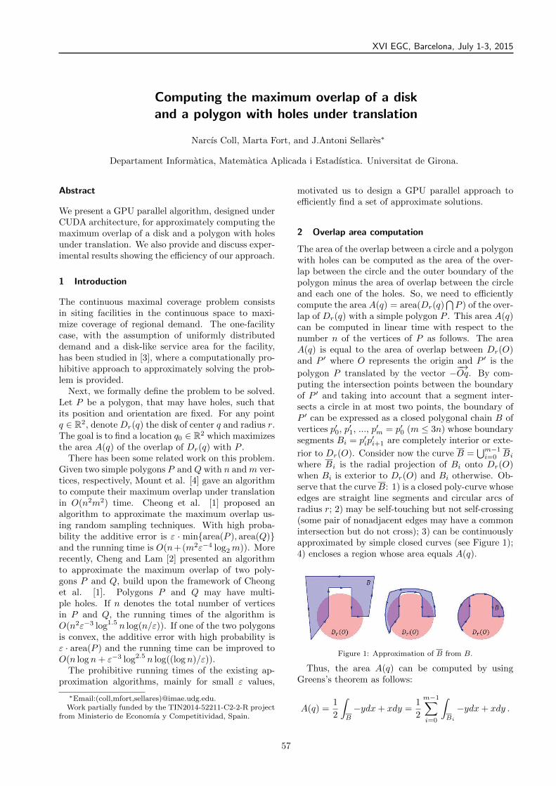
XVI EGC, Barcelona, July 1-3, 2015
Computing the maximum overlap of a diskand a polygon with holes under translation
Narcıs Coll, Marta Fort, and J.Antoni Sellares∗
Departament Informatica, Matematica Aplicada i Estadıstica. Universitat de Girona.
Abstract
We present a GPU parallel algorithm, designed underCUDA architecture, for approximately computing themaximum overlap of a disk and a polygon with holesunder translation. We also provide and discuss exper-imental results showing the efficiency of our approach.
1 Introduction
The continuous maximal coverage problem consistsin siting facilities in the continuous space to maxi-mize coverage of regional demand. The one-facilitycase, with the assumption of uniformly distributeddemand and a disk-like service area for the facility,has been studied in [3], where a computationally pro-hibitive approach to approximately solving the prob-lem is provided.
Next, we formally define the problem to be solved.Let P be a polygon, that may have holes, such thatits position and orientation are fixed. For any pointq ∈ R2, denote Dr(q) the disk of center q and radius r.The goal is to find a location q0 ∈ R2 which maximizesthe area A(q) of the overlap of Dr(q) with P .
There has been some related work on this problem.Given two simple polygons P and Q with n and m ver-tices, respectively, Mount et al. [4] gave an algorithmto compute their maximum overlap under translationin O(n2m2) time. Cheong et al. [1] proposed analgorithm to approximate the maximum overlap us-ing random sampling techniques. With high proba-bility the additive error is ε · minarea(P ), area(Q)and the running time is O(n+(m2ε−4 log2 m)). Morerecently, Cheng and Lam [2] presented an algorithmto approximate the maximum overlap of two poly-gons P and Q, build upon the framework of Cheonget al. [1]. Polygons P and Q may have multi-ple holes. If n denotes the total number of verticesin P and Q, the running times of the algorithm isO(n2ε−3 log1.5 n log(n/ε)). If one of the two polygonsis convex, the additive error with high probability isε · area(P ) and the running time can be improved toO(n log n + ε−3 log2.5 n log((log n)/ε)).
The prohibitive running times of the existing ap-proximation algorithms, mainly for small ε values,
∗Email:(coll,mfort,sellares)@imae.udg.edu.Work partially funded by the TIN2014-52211-C2-2-R project
from Ministerio de Economıa y Competitividad, Spain.
motivated us to design a GPU parallel approach toefficiently find a set of approximate solutions.
2 Overlap area computation
The area of the overlap between a circle and a polygonwith holes can be computed as the area of the over-lap between the circle and the outer boundary of thepolygon minus the area of overlap between the circleand each one of the holes. So, we need to efficientlycompute the area A(q) = area(Dr(q)
∩P ) of the over-
lap of Dr(q) with a simple polygon P . This area A(q)can be computed in linear time with respect to thenumber n of the vertices of P as follows. The areaA(q) is equal to the area of overlap between Dr(O)and P ′ where O represents the origin and P ′ is the
polygon P translated by the vector −−→Oq. By com-
puting the intersection points between the boundaryof P ′ and taking into account that a segment inter-sects a circle in at most two points, the boundary ofP ′ can be expressed as a closed polygonal chain B ofvertices p′
0, p′1, ..., p′
m = p′0 (m ≤ 3n) whose boundary
segments Bi = p′ip
′i+1 are completely interior or exte-
rior to Dr(O). Consider now the curve B =∪m−1
i=0 Bi
where Bi is the radial projection of Bi onto Dr(O)when Bi is exterior to Dr(O) and Bi otherwise. Ob-serve that the curve B: 1) is a closed poly-curve whoseedges are straight line segments and circular arcs ofradius r; 2) may be self-touching but not self-crossing(some pair of nonadjacent edges may have a commonintersection but do not cross); 3) can be continuouslyapproximated by simple closed curves (see Figure 1);4) encloses a region whose area equals A(q).
Figure 1: Approximation of B from B.
Thus, the area A(q) can be computed by usingGreens’s theorem as follows:
A(q) =1
2
∫
B
−ydx + xdy =1
2
m−1∑
i=0
∫
Bi
−ydx + xdy .
57

XVI Spanish Meeting on Computational Geometry
The value of the integral on Bi, Ii, depends onwhether Bi is interior or exterior to Dr(O). WhenBi is exterior, the arc Bi can be parameterized by:
(r cos(αi + t), r sin(αi + t)), t ∈ [0, αi,i+1] ,
where αi is the oriented angle between the vector−−→Op′
i
and the x axis and αi,i+1 is the oriented angle between
the vectors−−→Op′
i and−−−→Op′
i+1. Then, we have
Ii = r2αi,i+1 .
In the other case, that is, when Bi is interior to Dr(O),the segment Bi = Bi can be parameterized by:
p′i + t(p′
i+1 − pi), t ∈ [0, 1] .
Then, it holds:
Ii = det(p′i, p
′i+1) = det(pi − q, pi+1 − q) .
2.1 Acceleration of the overlap area computation
Consider that a piece of the chain B is completelyexterior to Dr(O) between the vertices p′
i and p′j (j >
i). Let Bi,j =∪j
k=i Bk be this piece of chain. Wewant to compute
Ii,j =
∫
Bi,j
−ydx + xdy =
j∑
k=i
Ik
without computing each Ik because it involves the usej − i times of the function arccos, which is computa-tionally expensive.
Let Aj,i be the shortest oriented arc on Dr(O) thatconnects the point p′
j with the point p′i and let Bi,i
be the closed simple curve determined by Bi,j ∪ Aj,i.Then, Ii,j can be computed by
Ii,j = Ii,i −∫
Aj,i
−ydx + xdy = Ii,i − r2αj,i ,
whereIi,i =
∫
Bi,i
−ydx + xdy ,
and αj,i denotes the oriented angle between the vec-
tors−−→Op′
j and−−→Op′
i.The result of the integral Ii,i depends on the ori-
entation of Bi,i and on whether the circle Dr(O) isinterior or exterior to Bi,i. Let ni,j be the number ofintersections between Bi,j and the half-line with ori-
gin O in the direction of the vector −−−→Op′
i. Accordingto ni,j and αji, there are three cases to consider (seeFigure 2):
1. ni,j is odd and αj,i > 0. Then, Dr(O) is interiorto Bi,i and Bi,i is oriented counterclockwise. Conse-quently, Ii,i = −2πr2 and Ii,j = r2(2π − αj,i).
2. ni,j is odd and αj,i < 0. Then, Dr(O) is interiorto Bi,i and Bi,i is oriented clockwise. Consequently,Ii,i = −2πr2 and Ii,j = −r2(2π + αj,i).
Figure 2: Exterior chain cases.
3. ni,j is even. Then, Dr(O) is exterior to Bi,i.Consequently, Ii,i = 0 and Ii,j = −r2αj,i.
In this way, for a chain of j − i vertices, we needto apply the intersection test between a segment anda half-line j − i times and we only need to use onetime the function arccos. Therefore, as we show inthe Results section, the time expended in the overlaparea computation decreases substantially.
3 Computing the maximum overlap
Lemma 1 At least a location optimizing A(q) be-longs to the region delimited by the convex hullCH(P ) of the simple polygon P and, consequently,it also belongs to the bounding box of P .
Proof. Assume that q0 is an optimal location suchthat q0 /∈ CH(P ), and denote q0 the closest point toq0 among all the points in CH(P ). When we translate
the disk Dr(q0) by the vector−−→q0q0 (see Figure 3) we
have that:
Dr(q0) ∩ CH(P ) ⊆ Dr(q0) . (1)
Taking into account that
Dr(q0) ∩ P ⊆ Dr(q0) ∩ CH(P ) , Dr(q0) ∩ P ⊆ P
and (1) we also have that:
Dr(q0) ∩ P ⊆ Dr(q0) ∩ P . (2)
From (2) we conclude that A(q0) ≥ A(q0).
To solve the problem we sample the bounding boxof the polygon P by using a uniform grid composedof square cells of side length d. Then, we compute thearea A(c) for each grid cell center c and pick a centerc0 with maximum area. To assure that the absoluteerror between areas when choosing as optimal grid
58

XVI EGC, Barcelona, July 1-3, 2015
Figure 3: Observe that Dr(q0) ∩ CH(P ) ⊆ Dr(q0).
center c0 instead of the optimal point q0 it is not toobad, we need to choose an appropriate side length dof the square grid cells.
Observe that the largest value of the absolute errorA(q0) − A(c0): 1) occurs when the point q0 coincideswith a vertex of a square grid cell; 2) is bounded by thearea of the lune L(q0) = Dr(q0) − (Dr(q0)
∩Dr(c)),
where c denotes a grid cell center, because the luneL(q0) is a subregion of Dr(q0)
∩P but the lune
L(c) = Dr(c) − (Dr(c)∩
Dr(q0)) does not intersectDr(q0)
∩P (see Figure 4a) and thus:
A(q0) − A(c0) ≤ A(q0) − A(c) ≤ area(L(q0)) . (3)
In the particular worst-case in which q0 is a ver-tex of the square grid cell of center c0, taking h =d(c0, q0) ≤ 2r, we have that:
h2 = 2d2
4; 2r ≥ h =
d√2; 8r2 − d2 ≥ 0 ,
and using Taylor expansion, we have:
area(L(q0)) = 2r2 arcsin
(h
2r
)+
h
2
√4r2 − h2 ≤
≤ 2rh =√
2dr .
Fixed r and ε ∈ (0, 1], and according to (3), a εabsolute error can be guaranteed by choosing the sidelength d of a square grid cell as
d = min
(2√
2r,ε√2r
),
because, in such a case:
A(q0) − A(c0) ≤ area(L(q0)) ≤√
2dr = ε .
Thus, if the bounding box of the polygon P hasdimension a × b, the number of vertices of the reg-ular grid providing an ε absolute error is (⌈a/d⌉ +1)(⌈b/d⌉ + 1) ∈ O(ab(r/ε)2).
When the maximum area of overlap A(q0) is at leasta sufficiently high fraction of the area of any disk ofradius r, we also obtain an (1−ε′)-approximation. Infact, assume A(q0) ≥ kπr2 for some k ≥ ε/(πr2) andtake 0 < ε′ = ε/(kπr2) ≤ 1, then ε = ε′kπr2 ≤ε′A(q0). Thus, from A(q0) − A(c0) ≤ ε we haveA(c0) ≥ A(q0) − ε ≥ A(q0) − ε′A(q0) = (1 − ε′)A(q0).
4 Adaptive local grid refinement
We can improve the accuracy of a solution obtainedwith an initial a×b grid by using a refinement method.An initial huge grid over the entire bounding box ofthe polygon P or a global refinement method wastesa lot of grid cells in areas where are not necessary.Using huge grids can be computationally demanding,both in terms of time and memory requirements, thuswe propose a local grid refinement method. This localgrid refinement strategy identifies the cells, called par-ent cells, to be refined according to a two-way filteringcriterium that allows us to quickly detect grid cellswhere it is not necessary to apply the refinement pro-cess because their points can not be optimal, Lemma2, or are all optimal, Lemma 3. After detecting theparent cells, we determine the new value for d, ac-cording to the desired ε or the maximum number ofdesired grid cells, and construct a new regular grid ofchild cells, over each selected parent cell. Finally, weperform for each child cell the process we followed forthe initial grid, this local refinement process can berepeated as many times as required until de desiredaccuracy is obtained.
Next, we give the mentioned Lemmas:
Lemma 2 If d ≤ 2√
2r and A(c0) − A(c) >√
2dr forthe center c of a grid cell g, then the optimal point q0
does not belongs to the cell g.
Proof. From (3) we know that if the cell g of centerc contains q0 the following inequalities are fulfilled:
A(q0) − A(c) ≤ area(L(q0)) ≤√
2dr . (4)
If A(c0) − A(c) >√
2dr, then also
A(q0) − A(c) ≥ A(c0) − A(c) >√
2dr , (5)
thus q0 cannot belong to g because in this case in-equalities (4) and (5) are in contradiction.
Lemma 3 Assume that: a) A(c) = area(Dr(c) ∩P ) = area(Dr(c)) = πr2, thus Dr(c) ⊆ P and c is anoptimal point; b) d ≤
√2r is fulfilled, hence, Dr(c)
covers the cell g. If for the center c′ of each one ofthe eight cells adjacent to cell g we have A(c′) = πr2,then any point of the cell g is optimal.
Proof. The union F of the set of all disks of radiusr whose center belongs to the cell g is the r-offset ofthe cell g. Consequently, if F ⊆ P , then, Dr(c
′) ⊆ Pfor any point c′ belonging to the cell g, thus c′ isan optimal point. Observe that the union of the eightdisks of radius r centered in the center of the grid cellsadjacent to cell g together with the disk Dr(c) coversthe r-offset F (see Figure 4b)). Thus, in order thatF ⊆ P it suffices that Dr(c
′) ⊆ P , or equivalentlyDr(c
′) = πr2, for the center c′ of each of the eightadjacent cells to g.
59

XVI Spanish Meeting on Computational Geometry
c
q0
L(c)
L(q0)
d
h
d
a) b)
Figure 4: a) The maximum error occurs when the optimal pointq0 is a vertex of a cell. b) The union of the nine disks coversthe cell offset.
5 GPU Implementation
The initial overlap areas, corresponding to the circlescentered at a a × b grid with d ≤
√2r, are computed
in parallel by finding one area per thread, the currentA(c0) value is estimated using an amortized atomicmax operation. The threads in a block cooperate tostore the polygon information to shared memory. Ifa refinement step is required, we analyze the cells inparallel using the filtering criteria, parent cells aremarked with a 1 and terminal cells with a 2 or a 0 de-pending on whether they are or can not be optimal. Itis done by using squared B ×B blocks, whose threadscooperate to transfer the B +2×B +2 potentially re-quired areas to shared memory. After being marked,the N parent cells are extracted and a k × k new gridis placed in each one. We take k = min(32, h, w, kε) inthe first step and k = min(32, k, kε) in the subsequentones; the 32 value is due to GPU reasons, and kε isthe required number of subdivisions needed to achieveε. However, we add two extra rows and columns sur-rounding the k × k grid, that will never be refined, tobe able to properly use the stop-refining criterium ofLemma 3 at this refinement step. Thus, we computek+2×k+2 areas per parent cell. Finally, the N(k+2)2
areas are computed in parallel and k × k blocks areused in the next filtering step, if it is required.
6 Experimental results
We have implemented our algorithms in C++ andCuda C and run the experiments using a Inter(R)Core(TM) i7-4790CPU with a Tesla k40 active GPU.
We have used the polygon with holes representingLos Angeles city map and considered the orange circleof Figure 5 of r = 6 (km). We can see, representedby colored points, the cell centers analyzed during theprocess. The green ones are the centers of the cellshaving maximum area, in this case πr2 ≈ 133 (km2).The blue points are the other analyzed centers, theyare painted in a blue color gradation according tothe overlap area of the circle centered on them. Thedarker the point the smaller the overlap area. Thegradual refinement is clearly seen in the figure as wellas some rounding errors in the points surrounding theregions with maximal area.
Figure 5: Los Angeles city map with the analyzed grid cellscenters, the optimal locations are marked in green. Initial gridsize=12 × 9.
Considering ε = 0.144 (km2) and a 12 × 9 initialgrid, which corresponds to an initial grid cell size ofd = 6.6 (km), the algorithm requires four refinementsteps and takes 0.35 (s), in this case the smallest gridcell size d is of 12 (m). If we start with a finer initialgrid of size 352 × 285, d = 0.2 (km), one refinementstep and 0.47 (s) are needed, now the smallest d is of16.6 (m). Thus, the adaptive local grid refinement isworthy, and the process to accelerate the area compu-tation too, if it is not used the running times become1.27 (s) and 1.56 (s).
References
[1] O. Cheong, A. Efrat, S. Har-Peled, Find-ing a guard that sees most and a shop thatsells most, Discrete & Computational Geometry37(4) (2007) 545-563.
[2] S.W. Cheng, C.K. Lam, Shape matching un-der rigid motion, Comput. Geom. Theory Appl.46(6) (2013) 591–603.
[3] T. C. Matisziw, A. T. Murray, Siting a facil-ity in continuous space to maximize coverage ofa region, Socio-Economic Planning Sciences 43(2009) 131-139.
[4] D.M. Mount, R. Silverman, A.Y. Wu, On thearea of overlap of translated polygons, ComputerVision and Image Understanding 64(1) (1996)53–61.
60

XVI EGC, Barcelona, July 1-3, 2015
The 2-center problem and ball operators in strictly convex normed planes
Pedro Martın∗1, Horst Martini†2, and Margarita Spirova‡3
1Departamento de Matematicas, Universidad de Extremadura2Fakultat fur Mathematik, TU Chemnitz
Abstract
We investigate the 2-center problem for arbitrarystrictly convex, centrally symmetric curves instead ofusual circles. In other words, we extend the 2-centerproblem (from the Euclidean plane) to strictly convexnormed planes. We show that the corresponding deci-sion problem can be solved in O(n2 log n) time, gener-alizing the algorithmical approach given by J. Hersh-berger for the Euclidean plane. In addition, we provevarious theorems on the notions of ball hull and ballintersection of finite sets in strictly convex normedplanes, which are fundamental for the 2-center prob-lem, but also interesting for themselves.
1 Introduction
The 2-center problem can be formulated as follows:given a (finite) set K of points in the plane, findtwo congruent closed discs of smallest possible radiuswhose union covers K. Variants of this problem arefrequently investigated, e.g., considering only centersfrom K (the so-called discrete 2-center problem), orby allowing two different radii. It is our aim to ex-tend this problem to arbitrary strictly convex normedplanes. Geometrically this means that we investi-gate the 2-center problem for arbitrary strictly con-vex, centrally symmetric curves instead of Euclideancircles. In addition, for a given radius λ > 0, we studygeometric properties of planar ball hulls (the inter-section of λ-balls containing K) and ball intersections(intersection of λ-balls whose centers belong to K).These notions are helpful for investigating (also algo-rithmically) the planar 2-center problem, and they areagain defined in the sense of strictly convex normedplanes.
From the more theoretical point of view, we obtainvarious new results on the ball hull and the ball inter-section of a finite set K in arbitrary strictly convexnormed planes. These results shed more light on the
∗Email: [email protected]. Research partially supportedby MICINN (Spain) and FEDER (UE) grant MTM2008-05460,and by Junta de Extremadura grant GR10060 (partially fi-nanced with FEDER).†Email: [email protected].‡Email: [email protected].
geometric structure of the boundary of such point setsassociated to K. Several lemmas and theorems herecan be considered as natural generalizations of resultsfrom [9] for the planar case (see also [11]). Further on,these results can be directly used for the constructionof planar ball hulls and ball intersections via circulararcs (in the sense of the respective norm), and theyare also useful for the algorithmical approach to the2-center problem presented in the final section, whichis a natural extension of that of J. Hershberger for theEuclidean subcase (cf. [7] and also [8]). Finally, weprove that, for two given radii and arbitrary strictlyconvex norms, the 2-center decision problem can besolved in O(n2 log n) time and O(n2) space.
2 Notation and preliminaries
Let Md = (Rd, ‖ · ‖) be a d-dimensional normed (orMinkowski) space. As is well-known, the unit ball Bof Md is a compact, convex set with non-empty in-terior (i.e., a convex body) centered at the origin o.The boundary of B is the unit sphere of Md, andany homothetical copy x+ λB of B is called the ballwith center x ∈ Rd and radius λ > 0 and denoted byB(x, λ); its boundary is the sphere S(x, λ).
Given a set of points K in M2 and λ > 0, the λ-ballhull bh(K,λ) of K is defined as the intersection of allballs of radius λ that contain K:
bh(K,λ) =⋂
K⊂B(x,λ)
B(x, λ).
Our Theorem 3 below describes the boundary struc-ture of bh(K,λ).
The λ-ball intersection bi(K,λ) of K is the inter-section of all balls of radius λ whose centers are fromK:
bi(K,λ) =⋂
x∈KB(x, λ).
Note that for d = 2 and K a finite set, the boundarystructure of bi(K,λ) consists of circular arcs of radiusλ with centers belonging to K.
Naturally, these notions make sense only ifbh(K,λ) 6= ∅ and bi(K,λ) 6= ∅, and this happensif and only if λ ≥ λK , where λK is the smallest num-ber such that K is contained in a translate of λKB.
61

XVI Spanish Meeting on Computational Geometry
The minimal enclosing ball of a bounded set is alwaysunique in the Euclidean subcase, but this is no truefor an arbitrary norm.
For a compact set K in Md denote by diam(K) :=max‖x−y‖ : x, y ∈ K the diameter of K. In whatfollows, when we speak about the λ-ball intersectionor λ-ball hull of a set K, we always mean that λ ≥ λK .It is easy to check (see also [2]) that
λK ≤ diam(K) ≤ 2λK .
3 On ball hulls of finite sets in the planar case
Let p and q be two points of the circle S(x, λ). In thefollowing, the minimal circular arc of B(x, λ) meetingp and q is the piece of S(x, λ) with endpoints p andq, which lies in the half-plane bounded by the line〈p, q〉 and not containing the center x. If p and qare opposite in S(x, λ), then the two half-circles withendpoints p and q are minimal circular arcs of S(x, λ)meeting p and q. We denote pq to a minimal circulararc meeting p and q .
Our objective in this section is to describe the struc-ture of the ball hull of a finite set K (see Theorem 3and Theorem 4). The proofs of the results in thissection are omitted but can be read in [10].
Lemma 1 Let M2 be a normed plane. Let p and qbe two points belonging to a disc of radius λ. If M2
is strictly convex or ‖p− q‖ ≤ λ, then
1. there exist only two minimal arcs of radius λmeeting p and q (which may degenerate to thesegment pq),
2. every disc of radius λ containing p and q also con-tains the minimal circular arcs of radius λ meet-ing p and q,
3. for every α ≥ λ, each disc of radius λ containingp and q also contains the minimal circular arcs ofradius α meeting p and q,
4. if a circular arc of radius λ meeting p and q iscontained in a disc of radius λ and contains inte-rior points of the disc, then this arc is a minimalcircular arc.
The above result is not true for normed planeswhich are not strictly convex and satisfy ‖p− q‖ > λ.With the maximum norm, the unit disc centered ato = (0, 0), the unit disc centered at x = (0.1, 0) andthe points p = (0.5, 1) and q = (0.5,−1) yield a coun-terexample.
Lemma 2 Let K = p1, p2, . . . , pn be a finite set ina normed plane M2 and λ > 0. If either the planeM2 is strictly convex or λ ≥ diam(K), then any disc
B(x, λ) which contains K also contains every minimalcircular arc of radius larger than or equal to λ andmeeting any two points pi and pj in K.
Theorem 3 Let K = p1, p2, . . . , pn be a finite setin a normed plane M2, and let λ ≥ λK . We denoteby pipj a minimal circular arc of radius λ meeting piand pj . Let H be the set of all discs of radius λ suchthat their boundary contains a circular arc meetingpoints from K. If the plane M2 is strictly convex orλ ≥ diam(K), then
bh(K,λ) =⋂
K⊂B(x,λ)∈HB(x, λ) = conv(
n⋃
i,j=1
pipj).
Theorem 3 shows that the boundary of the ball hullconsists of arcs meeting points fromK. The endpointsof such arcs are in fact extreme points of the ball hull.We call these points vertices of ball hulls.
Recall that the boundary of a planar ball intersec-tion consists of circular arcs. Similarly to vertices ofball hulls, we call their endpoints vertices of ball in-tersections.
Theorem 4 Let K = p1, p2, . . . , pn be a finite setin a normed plane M2 and λ ≥ λK . If M2 is strictlyconvex or λ ≥ diam(K), then every arc of the bound-ary of bi(K,λ) has a vertex of bh(K,λ) as center.Moreover, every vertex of bi(K,λ) is the center of anarc belonging to the boundary of bh(K,λ).
4 The algorithm for the 2-center problem
Given r1 > r2 > 0, the planar 2-center decision prob-lem asks whether a set K of n points in a normedplane can be covered by two discs of radius r1 andr2, respectively. Without loss of generality, we canassume that r ≡ r1 > r2 = 1. Of course, the consid-eration makes only sense when the diameter of K islarger than the radius r1, since otherwise a disc of ra-dius r1 covers K. Hershberger and Suri [8] publishedan algorithm solving the problem in O(n2 log n) timeand O(n) space in the Euclidean plane. Hershberger[7] improved the time cost to O(n2) using an algo-rithm described by Step 1 and Step 2:
Step 1. Building the arrangement of discs withradius r centered at the points of K.
Step 2. Moving a reference point p along theboundary of the discs from the arrangement, keep-ing track of the set F of points that are farther thana distance r away.
For describing precisely the idea from [7], let pθ (θ ∈[0, 360o]) be a parametrization of a disc C from thearrangement, and consider four disjoints sweeps in thecircle. Let [θ1, θ1 + 90o) be one of those sweeps. Forevery θ ∈ [θ1, θ1 + 90o), define the following variablesets:
62

XVI EGC, Barcelona, July 1-3, 2015
Fθ: the points of K which do not belong to the disccentered at pθ;Dθ: the points of K which do not belong to the
disc centered at pθ and do not belong to the discscentered at other previous (in the oriented sense ofthe parametrization of the circle) points.Aθ: the points of K which do not belong to the
disc centered at pθ, but each of them belongs to somedisc centered at other previous (in the oriented senseof the parametrization of the circle) points.
Obviously, Fθ = Dθ ∪ Aθ for every θ. Move pθalong the sweep starting with θ = θ1. The sets Fθ, Dθ
and Aθ may change. At the beginning we have Fθ =Dθ, and Aθ is empty. When pθ moves, some pointsare possibly deleted in Dθ, because they leave Fθ.Nevertheless, some points possibly begin to belong toAθ when they begin to belong (again or for the firsttime) to Fθ.
After each change to Aθ and Dθ, test whetherbi(Aθ, 1) and bi(Dθ, 1) intersect. The point pθ andevery point of this (eventually) non-empty intersec-tion become the centers of a solution pair of discs forthe 2-center problem. Therefore, for each circle C, foreach of the four 90o arcs that cover C:
Step 2(a). Find the order of insertions and dele-tions to Aθ and Dθ in O(n) time by walking along theboundary of C.
Step 2(b). Process the insertions to Aθ in se-quence, maintaining bi(Aθ, 1). Record the changesto bi(Aθ, 1) in a transcript.
Step 2(c). Partition of the initial set Dθ1 into astatic set Z of points that will not be deleted duringthe sweep, and a dynamic set Yθ of points that willbe deleted.
Step 2(d). Play the transcripts for Aθ and Dθ
simultaneously, both in forward time order (the re-verse of the construction order for Dθ). Test whetherbi(Aθ, 1) and bi(Dθ, 1) overlap at any point duringthe playback.
In the following, we justify that Hersberger’s ap-proach runs correctly in a strictly convex normedplane, and finally we obtain Theorem 10.
Lemma 5 Let M2 be a strictly convex normed plane.If K is a set of n points in M2, then, building thearrangement of circles with radius r > 0 centered atthe points of K takes O(n2 log n) time and O(n2)space.
Proof. The circles are well behaved, i.e., the totalnumber of intersections is O(n2) and the calculation ofthe intersection points of two circles is a basic opera-tion in our process and takes constant time. Thus, thearrangement can be constructed in O((n + k) log n)time using (the output sensitive) plane-sweep algo-rithm (see [6]), where k = O(n2) is the number of
intersections between the circles. The space is obvi-ously O(n2).
Lemma 6 Let M2 be a strictly convex normedplane, and p1, p2, . . . , pm be the points added to Aθin order of addition when p moves during its 90o
sweep. Suppose that each arc on the boundary ofbi(p1, p2, . . . , pj, 1) is labelled with an integer i ifthe arc belongs to the disc centered at pi. Then, forany j, the labels of the arcs of bi(p1, p2, . . . , pj, 1)form a circular sequence with no duplication, one localmaximum, and one local minimum.
Proof. Lemma 1 in [7] proves the statement in theEuclidean case making use of the following argumentsthat we prove for strictly convex normed planes:
1) Every arc from the boundary of bi(K, r) is gen-erated by a vertex on the boundary of bh(K, r), andevery vertex on bi(K, r) corresponds to an arc fromthe boundary of bh(K, r). This is our Theorem 4.
2) If r ≥ 1, then bh(K, r) ⊆ bh(K, 1). This isproved, for instead, in [9].
3) Let B(x1, 1) and B(x2, 1) be two discs in anormed plane M2 whose intersection has non-emptyinterior. Let t3 be a point belonging to S(x1, 1) ∩S(x2, 1). Let us consider a third circle S of radius1 containing t3. This third circle cannot simultane-ously contain points of both the arcs which form theboundary of B(x1, 1) ∩B(x2, 1).
4) If a point b belongs to the convex hull of threepoints a, c, d, then b is not a vertex of the ball hullof a, b, c, d of radius r.
Due to the structure of the boundary of the ballintersection and its non-increasing property whenpoints are added (see [9]), the proofs presented in [7]of the following Theorem 7, Theorem 8, and Theorem9 are also valid for any strictly convex normed planeusing Lemma 6.
Theorem 7 We can maintain bi(Aθ, 1) as Aθ growsin O(|A|) total time, where |A| is the final cardinalityof Aθ.
Theorem 8 Let M2 be a strictly convex normedplane. Let Z be a fixed set of points, and Yθ be adynamic set subject to deletions only. Suppose weknow the x-sorted order of Yθ and Z, and suppose weare given a change-transcript for bi(Yθ, 1). Then wecan compute a change-transcript for bi(Yθ∪Z, 1) withO(|Yθ|+ |Z|) additional work.
Theorem 9 Let M2 be a strictly convex normedplane. Let Aθ and Dθ be two sets of points subjectto insertions and deletions only, respectively. Sup-pose that some oracle maintains the boundaries ofbi(Aθ, 1) and bi(Dθ, 1) in a linked-list form, and thatat each update it gives us a pointer to the changed
63

XVI Spanish Meeting on Computational Geometry
edges. Then we can detect when, if ever, bi(Aθ, 1)and bi(Dθ, 1) intersect, using O(|Aθ|+ |Dθ|) time al-together, where |Aθ| and |Dθ| are the maximum car-dinalities of Aθ and Dθ.
Finally we obtain our main result in this section.
Theorem 10 In any strictly convex normed plane,the generalized planar 2-center decision problem canbe solved in O(n2 log n) time and O(n2) space.
Proof. Lemma 5 supports Step 1 in a strictly convexnormed plane. Theorem 7 shows that Step 2(b) runsin O(|A|) total time, where |A| is the final cardinalityof Aθ. For Step 2(c), use the algorithm of Theorem7 to compute a change-transcript for bi(Yθ, 1), work-ing in time-reversed order; using Theorem 8, combinethis with Z to get a change-transcript for bi(Dθ, 1).Theorem 9 proves that Step 2(d) can be done in O(n)time.
Observation 1 Chazelle and Lee [3] proved that forgiven n points p1, ..., pn and a fixed disc of radius r,the arrangement of Euclidean circles with radius rcentered at these points can be constructed in O(n2)time and space, and this allows to obtain in [7] a bet-ter final bound for the Euclidean two center problem.
Observation 2 We can rewrite our Theorem 10 us-ing the following from [5]. Let there be given a set ofn curves, where each pair of curves can have at most sintersection points, for a constant s. In this case, thezone complexity of a single curve is O(λs+2(n)), whereλσ(k) denotes the maximal length of a Davenport-Schinzel sequence of k elements with order σ. Thus,the total construction time is O(nλs+2(n)), while thecomplexity of the arrangement is of course O(n2).Due to s = 2 for strictly convex normed planes, ourTheorem 10 can be formulated as follows: the gener-alized planar 2-center decision problem can be solvedin O(nλ4(n)) time and O(n2) space in any strictlyconvex normed plane. It is important to note thatλσ(k) is almost linear in k for small values of σ (forDavenport-Schinzel sequences see [1] and [12]).
References
[1] P.K. Agarwal, M. Sharir, and P. Shor, Sharp upperand lower bounds on the length of general Davenport-Schinzel sequences, Journal of Combinatorial Theory,Series A, 52 (1989), 228–274.
[2] M. Baronti, and L.P. Papini, Diameters, centersand diametrically maximal sets, Rend. Circ. Mat.Palermo Suppl. 38 (1995), 11–24.
[3] B. Chazelle, and D.T. Lee, On a circle placementproblem, Computing 36 (1986), 1–16.
[4] B. Grunbaum, Borsuk’s partition conjecture inMinkowski planes, Bull. Res. Council Israel, Sect. F7F (1957/1958), 25–30.
[5] E. Fogel, D. Halperin, L. Kettner, M. Teillaud, R.Wein, and N. Wolpert, Arrangements, in: EffectiveComputational Geometry for Curves and Surfaces,J.D. Boissonnat and M. Teillaud (editors), Mathe-matics and Visualization, Springer-Verlag, 2006, 1–66.
[6] E. Fogel, D. Halperin, and R. Wein, CGAL Arrange-ments and Their Applications. A Step-by-Step Guide,Springer, 2012.
[7] J. Hershberger, A faster algorithm for the two-centerdecision problem, Inform. Process. Lett. 47 (1993),23–29.
[8] J. Hershberger, and S. Suri, Finding tailored parti-tions, J. Algorithms 12 (1991), 431–463.
[9] P. Martın, H. Martini, and M. Spirova, Chebyshevsets and ball operators, J. Convex Anal. 21 (2014),601-618.
[10] P. Martın, H. Martini, M. Spirova: The 2-centerproblem and ball operators in strictly convex normedplanes, submitted, http://arxiv.org/abs/1409.8055.
[11] H. Martini, and M. Spirova, On the circular hullproperty in normed planes, Acta Math. Hungar. 125(2009), 275-285.
[12] G. Nivasch, Improved bounds and new techniques forDavenport-Schinzel sequences and their generaliza-tions, Journal of the ACM 57 (2010), article 17, 44pages.
[13] M. Sharir, A near-linear algorithm for the planar 2-center problem, Discrete Comput. Geom. 18 (1997),125–134.
64

XVI EGC, Barcelona, July 1-3, 2015
Combining surface and volume Reeb graphs for solid segmentation
B. Strodthoff∗1 and B. Juttler1
1Johannes Kepler University, Linz, Austria
Abstract
The Reeb graph captures the structure of a domainusing a scalar-valued function defined on it. For asolid object, one can distinguish between the Reebgraph of the object’s volume and the Reeb graphof its boundary surface. In general, the surface andvolume Reeb graph are different objects, where eachhas its advantages and disadvantages for analyzing ashape. We propose a combination of both, which, fora certain class of defining functions, can be computedfrom a boundary description of the object and cap-tures more information about its structure than theindividual graphs. As an application, we present avolume decomposition algorithm guided by the com-bined surface volume Reeb graph.
Introduction
The Reeb graph captures the structure of an objectefficiently by tracking the level-set components of ascalar-valued function defined on the object. There-fore, the Reeb graph typically finds applications inshape analysis, simplification or decomposition.
For a solid object, two different Reeb graphs canbe considered. The volume Reeb graph (VRG) tracksthe level set components of the function restricted tothe object (considered as 3-dimensional manifold withboundary). Typically its construction requires a vol-umetric description of the object. Also, the volumeReeb graph does not recognize holes in level set com-ponents and thus may neglect some important struc-tural features of the object.
Tracking the level set components of the functionrestricted to the boundary surface of the object in-stead leads to the surface Reeb graph (SRG). It canbe computed efficiently from a surface representationof the object. When using a suitable function, such asthe height function or the average geodesic distancefunction, the SRG is also able to capture the structureof certain objects. More precisely, this is the case forobjects that contain substantial protrusions (such asthe limbs of an animal or the trunks of a tree) butno significant cavities (such as the inner boundary of
∗Email: [email protected]. Research supported bythe Austrian Science Fund (FWF) through NFN S117 “Ge-ometry + Simulation”
a vase or cup). For suitable objects, for example, asurface decomposition guided by the SRG can be ex-tended to a meaningful decomposition of the objectby inserting cutting surfaces between the boundarycurves of surface patches. For other objects, the in-sertion of these surfaces may intersect the boundarysurface or lead to a decomposition of the object intoless satisfactory parts.
We propose the surface volume Reeb graph (SVRG)that combines the advantages of the SRG and theVRG. For a certain class of defining functions, it canbe computed efficiently from a surface description ofthe object and captures the information of both indi-vidual structures. As an application, we present a vol-ume decomposition algorithm guided by the SVRG,which is able to decompose complicated objects (in-cluding objects with deep cavities and holes) intopieces that are easier to parametrize.
Our solid segmentation is guided by Reeb graphs(see e.g. [2, 7, 8]) with respect to one or several Morsefunctions.
The SRG has been used repeatedly for analyz-ing and decomposing boundary surfaces of objects[1, 14, 15], typically using the average geodesic dis-tance function [1, 15] or geodesic distances to featurepoints [14].
Also the VRG has been used to analyze and decom-pose objects [16, 12], although it does not recognizeholes appearing in a level set component. By includ-ing a second defining function, the VRG is generalizedto the Reeb space, which captures more details of theobject [7, 11], however at the price of being more ex-pensive to compute.
The close relation between the genus of a surfaceand its Reeb graph is investigated in [3]. Extend-ing this idea, surface Reeb graphs were used to detecthandle and tunnel loops of an object in boundary rep-resentation [4]. Finally, cutting surfaces are insertedinto an object in order to get objects with cycle-freeReeb graphs in [6, 13]. This reduces the genus, butsome holes may remain in the object.
Several algorithms are described in the literaturethat compute the Reeb graph of a surface for a givensurface description, or the Reeb graph of a volumefor a given volumetric description (e.g. [5, 9, 10, 13]).These algorithms typically allow for a general choiceof defining functions, but if a three-dimensional man-
65

XVI Spanish Meeting on Computational Geometry
ifold is given in a boundary description only, a volu-metric description (such as a tetrahedral mesh) has tobe generated first to compute the VRG. To avoid this,we compute both Reeb graphs using an algorithm thatworks on the boundary representation, see [11, 12]and Section 1.3. However, it should be noted that theboundary-based construction limits the choice of theMorse function.
1 The surface volume Reeb graph (SVRG)
After recalling the definition of Reeb graphs, we intro-duce the surface volume Reeb graph, which combinestwo Reeb graphs of a solid object.
1.1 Reeb graphs
We begin by recalling the definition of Reeb graphs(see [2] for a more detailed and general introduction).
Definition 1 Consider a scalar-valued function f de-fined on a d-manifold (or a manifold with boundary)M . Points mapped to the same function value form alevel set, connected parts of a level set are called levelset components. The Reeb graph of M with respectto f is obtained by contracting every level set compo-nent to a point, maintaining adjacency between levelsets.
For a solid object, two different Reeb graphs can beconsidered, see also Figure 1. On the one hand, onecan consider a function defined on the object consid-ered as 3-manifold with boundary. We will call theReeb graph generated by this function the VolumeReeb graph (VRG). On the other hand, consider afunction defined on the surface of the object. Thelevel set components of such a function consist ofcurves on the boundary of the object. The Reeb graphtracing these level set components will be denoted asSurface Reeb graph (SRG) in the following.
1.2 The combined surface volume Reeb graph
Motivated by the close relations between the SRG andthe VRG, we introduce a combined structure, the sur-face volume Reeb graph, see also Figure 1. While theVRG does not recognize holes appearing in level sets,and the SRG does not know which boundary compo-nents bound the same level set component, the SVRGcombines the structural information of both graphs.
Definition 2 To form the combined surface and vol-ume Reeb graph (SVRG), the edges of the SRG aresubdivided into edge segments at the f -values of in-cident vertices of the VRG. Each edge segment is la-beled by the associated edges of the VRG.
66
5
4
3
2
1
6
5
4
3
2
1
4
1
2
3
5
6
5
1
3
SVRGVRGSRGlevelsetsthe object
d
c
b b
aa
d
d
c
d
cc
Figure 1: Surface Reeb graph (SRG), Volume Reebgraph (VRG) and their combination (SVRG) with re-spect to the height function, which maps every pointto its last coordinate. The VRG contains only onecycle corresponding to the handle on the left. In theSRG, also the vertical hole induces a cycle, since theboundary curve splits into an inner and an outer com-ponent. The SVRG combines the information of theother two graphs. Note that the inner boundary com-ponent connecting points 2 and 4 is split into two edgesegments with different labels.
For every edge segment, a connected, monotonepath of mesh-edges is stored. The edges of the SRGand the VRG are represented by lists of such edgesegments, where every edge segment stores referencesto the containing edges.
The vertices of the SVRG contain an instance ofa SRG-vertex and, additionally, a VRG-vertex whereappropriate. Those have access to the incident edgesof the SRG and VRG, respectively. Additionally, avertex of the SVRG stores a reference to the underly-ing vertex of the surface mesh and a set of the orientedlevel set polygons through v, which can be traced effi-ciently. Using only these polygons and their orienta-tion, we can decide what kind of vertex of the SVRGlies in v.
1.3 Computation of the SVRG from a boundaryrepresentation
The SVRG is computed efficiently from a triangulatedboundary mesh of the given object, using an adapta-tion of the algorithm presented in [12], see Algorithm1. We use a sweep algorithm where the status con-tains all edge segments at the current function level.The events of the sweep are the vertices of the SVRG.Those always lie in critical vertices of the mesh, i.e.in local minima, maxima and saddle points with re-spect to f , and can thus be located by considering theincident triangles.
In order to identify whether an edge segment in thestatus is influenced by a vertex V , we use the levelset polygons through v. Typically, the level set poly-gons are, at some point, intersected by the mesh-edgesrepresenting the edge segment. Only in a minimum V
66

XVI EGC, Barcelona, July 1-3, 2015
Algorithm 1 computeSVRG
for all vertices v of mesh doif v is critical with respect to f then
trace oriented level set polygons through vcreate a SVRG-vertex V (v)add V to vertex list
sort vertex list by increasing f -valuefor all V in vertex list do
grow edge segments to the f -value of Videntify influenced edge segments in statusupdate status and SVRG
that is no vertex of the VRG, we trace level set poly-gons starting from the edge segments in the statusand check which one surrounds V .
2 SVRG-guided volume segmentation
We show an application of the SVRG to guide thedecomposition of solid objects into pieces that areeasier to parametrize. More precisely, we are inter-ested in trivariate tensor-product spline parameteri-zations, which are able to represent topological hex-ahedra, since their domain is the unit cube. Thus,ideally we would get hexahedral pieces, but we willaim for contractible volumes that can be segmentedinto few hexahedral volumes efficiently in a secondstep.
2.1 Reeb graphs for volume segmentations
For simple objects, surface decompositions based onthe SRG can often be extended to satisfactory de-compositions of the volume. In general, however, asurface segmentation may contain patches describingthe boundary surfaces of holes or deep cavities, andthus does not induce a valid volume decomposition.Decomposition algorithms based on the VRG alwaysgive valid volume segmentations, eg. [16]. However,the computation of the VRG is typically more expen-sive than the SRG-construction, requiring a volumemesh of the object.
The surface Reeb graph (and therefore also theSVRG) has a close relation to the genus of the under-lying object. Every hole of the object is representedby a loop in the SRG [3]. The loops of the VRG are,typically, a subset of the loops of the SRG. An ob-ject decomposition algorithm guided by Reeb graphsshould therefore aim at a reduction of the number ofloops of the graph.
In [6, 13], the object is cut along level sets of thedefining function in order to resolve the loops of theVRG. The aim of those works is to reduce the con-struction of the volume Reeb graph to the much moreefficient construction of the contour tree, its loop-freeequivalent. Since cutting surfaces are, thus, only in-
serted symbolically, it is not necessary to optimizetheir quality.
We apply the SVRG to obtain a decomposition ofthe object. The VRG guides the volume decompo-sition, while the contained SRG gives efficient accessto the boundary components of an inserted cuttingsurface. While cutting along level sets of the defin-ing functions as in [6, 13], we aim at cuts comply-ing with a certain quality criterion to achieve nicelyshaped pieces. Also, we do not only insert the mini-mum number of cuts to resolve loops of the VRG, butadd more cuts if they simplify the resulting pieces.Finally, we repeatedly use this approach for differentdefining functions.
The Reeb graph may be complicated due to manysuperfluous small branches. In the VRG contained inour SVRG, we cut away those small branches up to acertain threshold and merge edges in resulting verticesof valency two. The resulting reduced volume Reebgraph (VRG*) is used to guide the construction.
2.2 The cutting algorithm
We begin by giving an overview of the overallalgorithm, see Algorithm 2. The algorithm hasbeen fully implemented in C++ based on theComputational Geometry Algorithms Library CGAL(www.cgal.org).
Algorithm 2 cutObject
while not finished doChoose function f and quality bound q.Compute SVRG and VRG*.for all edges of VRG* do
use SVRG to get good cut candidate.
sort edges by the quality of their cut candidates.for all edges e of VRG*, starting at best do
if quality of e > q thenif cutting e simplifies the SVRG then
add e to cut edges.
Reject cut edges that do not split the objectImplement cuts of remaining cut edges
In every iteration of the algorithm, we first choosea function f and a quality bound q. The qualitybound will be set rather high in the beginning, aimingat high-quality cutting surfaces. In short, we prefercutting surfaces that have few boundary componentsand which form near-orthogonal intersections with thesurrounding object surface. In subsequent iterations,we decrease the quality bound to make sure that suf-ficiently many cuts are eventually accepted.
For the function f , we start with some given func-tions. In later iterations, we can use the SRG of aprevious iteration to estimate the axis of a hole in theobject, which enables us to generate a function for thenext iteration that is able to resolve that hole.
67

XVI Spanish Meeting on Computational Geometry
After choosing f and q appropriately, the sur-face volume Reeb graph SVRG is computed using aboundary-based construction algorithm as describedin Section 1.3. We then compute a good candidatecutting surface for every edge of the VRG* and sortthe edges by their quality.
First, an initial set of good cuts is generated. Start-ing from the edges allowing the best cuts, we greedilyselect cut edges if neither of their ends has valencyone. In the following step, some of the previouslyselected cut edges are rejected if the correspondingcutting surfaces would be inserted into one of the re-sulting pieces instead of splitting the object.
We present some exemplary results of our decom-position algorithm in Fig. 2.
Figure 2: Results of our decomposition algorithm.
3 Conclusion
We presented a novel algorithm for decomposing solidobjects into simpler pieces. Given a Morse functionf we combine the Reeb graphs of the object’s volumeand of its boundary surface. We then examine theedges of the contained volume Reeb graph. If theirremoval helps us to split the object – and this can bedecided using the Reeb graph – then we cut it with alevel set of f . In order to optimize the quality of theresulting pieces, a quality criterion is applied duringthe selection of cutting surfaces. This procedure isrepeated using different functions f .
In our examples, the presented method generatessatisfactory decompositions. The user can control thequality of the resulting shapes by using different start-ing functions or different bounds for accepting cuttingsurfaces.
The choice of suitable Morse functions remains aninteresting topic for future research. So far we haveused only linear functions. In order to allow curvedcutting surfaces, the approach could be generalizedto nonlinear functions, provided that they allow for aboundary-based construction of the Reeb graphs.
References
[1] S. Berretti, A. del Bimbo, and P. Pala. 3D Meshdecomposition using Reeb graphs. Image and VisionComputing, 27:1540–1544, 2009.
[2] S. Biasotti, D. Giorgi, M. Spagnuolo, and B. Falci-dieno. Reeb graphs for shape analysis and applica-tions. Theor. Computer Science, 392(1-3):5–22, 2008.
[3] K. Cole-McLaughlin, H. Edelsbrunner, J. Harer,V. Natarajan, and V. Pascucci. Loops in Reeb graphsof 2-manifolds. Discr. Comput. Geom., 32(2):231–244, 2004.
[4] T. K. Dey, F. Fan, and Y. Wang. An efficient com-putation of handle and tunnel loops via Reeb graphs.ACM Trans. Graph., 32(4):32:1–32:10, 2013.
[5] H. Doraiswamy and V. Natarajan. Efficient algo-rithms for computing Reeb graphs. Comput. Geom.,42(6-7):606–616, 2009.
[6] H. Doraiswamy and V. Natarajan. Computing Reebgraphs as a union of contour trees. IEEE Trans. Vis.Comp. Graph., 19(2):249–262, 2013.
[7] H. Edelsbrunner, J. Harer, and A. K. Patel. Reebspaces of piecewise linear mappings. In Proc. Symp.Comput. Geom., pages 242–250. ACM, 2008.
[8] M. Hilaga, Y. Shinagawa, T. Kohmura, and T. Ku-nii. Topology matching for fully automatic similarityestimation of 3D shapes. In Proc. SIGGRAPH Conf.Computer Graphics, pages 203–212. ACM, 2001.
[9] V. Pascucci, G. Scorzelli, P.-T. Bremer, and A. Mas-carenhas. Robust on-line computation of Reebgraphs: Simplicity and speed. ACM Trans. Graph.,26(3), 2007. article no. 58.
[10] G. Patane, M. Spagnuolo, and B. Falcidieno. Aminimal contouring approach to the computation ofthe Reeb graph. IEEE Trans. Vis. Comp. Graph.,15(4):583–595, 2009.
[11] B. Strodthoff and B. Juttler. Layered Reeb graphsfor three-dimensional manifolds in boundary repre-sentation. Computers & Graphics, 46:186–197, 2015.
[12] B. Strodthoff, M. Schifko, and B. Juttler. Horizon-tal decomposition of triangulated solids for the sim-ulation of dip-coating processes. Comp.-Aided Des.,43:1891–1901, 2011.
[13] J. Tierny, A. Gyulassy, E. Simon, and V. Pascucci.Loop surgery for volumetric meshes: Reeb graphsreduced to contour trees. IEEE Trans. Vis. Comp.Graph., 15(6):1177–1184, 2009.
[14] J. Tierny, J.-P. Vandeborre, and M. Daoudi. Topol-ogy driven 3d mesh hierarchical segmentation. InIEEE Shape Modeling and Applications, pages 215–220, 2007.
[15] E. Zhang, K. Mischaikow, and G. Turk. Feature-based surface parameterization and texture mapping.ACM Trans. Graph., 24:1–27, 2005.
[16] X. Zhang, J. Liu, Z. Li, and M. Jaeger. Volumedecomposition and hierarchical skeletonization. InProc. SIGGRAPH Int. Conf. Virtual-Reality Contin-uum and Its Applications in Industry, pages 17:1–17:6. ACM, 2008.
68

XVI EGC, Barcelona, July 1-3, 2015
Minimum interference graph coloring and monochromatic edges
Javier Lorenzo-Diaz∗1, David Orden†2, Ivan Marsa-Maestre‡3, Jose Manuel Gimenez-Guzman§3, and Enriquede la Hoz ¶3
1Grado en Ingenierıa Telematica, Universidad de Alcala2Departamento de Fısica y Matematicas, Universidad de Alcala
3Departamento de Automatica, Universidad de Alcala
Abstract
Motivated by WiFi channel assignment, we considera graph together with a spectrum of colors and amatrix of interferences between colors. We exploretwo vertex-coloring problems. First, the Thresh-old Spectrum Coloring problem: allowing a fixednumber of colors, it aims to minimize the maximumof the interferences at the vertices. Second, theChromatic Spectrum Coloring problem: fixinga threshold and allowing to use as many colors as ver-tices, it aims to minimize the number of colors lead-ing to an interference below the threshold at everyvertex. To deal with these problems, we have im-plemented modifications of the well-known DSATURheuristic to account for the given spectrum, compar-ing their results with those of the heuristic optimiza-tion algorithm ALHSO. Further, we have checked theappearance of monochromatic edges in the coloringsobtained.
1 Introduction
Graph coloring is among the main problems in Dis-crete Mathematics, attracting researchers because ofboth theoretical challenges and applications [8, 12].One of the most prominent vertex-coloring prob-lems is frequency assignment [1], for which modelsrange from the most naive, forbidding monochro-matic edges, to the most general, with assignmentconstraints, interference constraints, and an objectivefunction.
The present work explores an intermediate model,
∗Email: [email protected]. Research supported byMECD Beca de colaboracion en departamentos.†Email: [email protected]. Research supported
by MICINN Project MTM2011-22792, ATLAS-ProjectVA172A12-2, and TIGRE5-CM Comunidad de Madrid ProjectS2013/ICE-2919.‡Email: [email protected]. Research supported by
TIGRE5-CM Comunidad de Madrid Project S2013/ICE-2919§Email: [email protected]. Research supported by
TIGRE5-CM Comunidad de Madrid Project S2013/ICE-2919¶Email: [email protected]. Research supported by
TIGRE5-CM Comunidad de Madrid Project S2013/ICE-2919
in which we are given a graph G and a spectrum ofcolors S = c1, . . . , cs endorsed with a matrix W ofnon-negative interferences Wij = W (ci, cj) betweeneach pair of colors. For such a pair (G,W ), a col-oring c of the graph will induce at each vertex v aninterference Iv(G,W, c) =
∑u∈N(v)W (c(u), c(v)).
This is motivated by the setting in IEEE 802.11-based wireless access technology, commonly known asWiFi, in which each access point must be assigned afrequency channel from a given spectrum, where in-terferences between channels arise and one aims tominimize the interference at access points. Havingthis in mind, we introduce the Threshold Spec-trum Coloring (TSC) problem: fixed a spectrumof k colors, endorsed with a k × k matrix W of in-terferences between colors, the goal is to determinethe minimum threshold t ∈ R≥0 such that (G,W ) ad-mits a k-coloring c in which the interference at everyvertex is at most t, i.e., Iv(G,W, c) ≤ t, ∀v. Such aminimum t will be called the minimum k-chromaticthreshold of (G,W ), denoted as Tk(G,W ).
For a counterpart, we also consider the Chro-matic Spectrum Coloring (CSC) problem: fixeda threshold t ∈ R≥0 and letting the spectrum to havesize |V (G)|, the goal is to determine the minimumnumber of colors k ∈ N such that (G,W ) admits ak-coloring c in which the interference at every vertexis at most that threshold t. Such a minimum k will becalled the t-interference chromatic number of (G,W ),denoted as χt(G,W ).
Observe that the usual Vertex Coloring prob-lem is the particular case with the identity as ma-trix of weights and a threshold t = 0, i.e., χ(G) =χ0(G, I). With the same matrix and a threshold twe get the Improper Coloring problem, which al-lows at most t monochromatic edges around a vertex.These two particular cases are NP-hard [6, 13], henceso is the Chromatic Spectrum Coloring problem.
In addition, fixed any k ≥ 2 it is NP-complete todecide if there exists a k-coloring with interference atmost any threshold t ≥ 2, see [3] and the referencestherein. Hence, the Threshold Spectrum Color-ing is also NP-hard.
69

XVI Spanish Meeting on Computational Geometry
2 Related work
Araujo et al. [3] considered a weight function w onthe edges of the graph G instead of a matrix W ofinterferences between colors, and they define the in-terference at a vertex to be the sum of weights of inci-dent monochromatic edges. For a given edge-weightedgraph (G,w) they study the Weighted ImproperColoring in which, fixed a threshold t ∈ R≥0, thegoal is to determine the minimum number of col-ors k ∈ N such that (G,w) admits a k-coloring cin which the interference at every vertex is at mostthat threshold t. They also study the ThresholdImproper Coloring problem, where fixed a spec-trum of k colors the goal is to determine the mini-mum threshold t ∈ R≥0 such that (G,w) admits ak-coloring c in which the interference at every vertexis at most t.
Of independent interest are the works on theFrequency Assignment Problem, which use differentmodels to fit the characteristics of specific applica-tions. An interested reader can check the survey byAardal et al. [1].
3 Experiments
We have conducted a first experimental analysis ofour two problems, based on benchmarking differenttechniques in a range of scenarios. In this section wedescribe these scenarios, summarizing the techniqueswe have tested in them, and discussing the resultsobtained in the experiments.
3.1 Settings
As an initial exploration of the problem space, wehave considered graphs generated randomly using theErdos-Renyi (ER) model [7]. In it, every pair ofvertices has a prescribed probability p of being con-nected. Different sub-categories were created by vary-ing the number of vertices n and the probability ofconnection p. In particular, we generated 10 graphsfor each combination of the following parameters:number of vertices n ∈ 60, 70, 80 and probability ofconnection p ∈ 0.1, 0.3, 0.5, 0.7, 0.9, which are thesame settings used in [9, 10].
For the interference between colors we have consid-ered an exponential decay of base 2 with the position
of the colors in the list, i.e., Wij =1
2|i−j|
3.2 Coloring techniques used for benchmarking
For a first experimental analysis of our two prob-lems, we have adapted the sequential greedy algo-rithm DSATUR [4], standard for the usual Ver-tex Coloring problem. Our implementation TSC-DSATUR for the Threshold Spectrum Coloring
problem looks for the color minimizing the interfer-ence at v. Our implementation CSC-DSATUR for theChromatic Spectrum Coloring problem looks fora color that does not make interference at v exceedthe product of the fixed threshold t by the propor-tion of neighbors already colored. That is, if vertex vhas five neighbours, but only three of them have beencolored so far, the color chosen should guarantee theinterference at v to be at most 3
5 t. For a color to bechosen, this constraint must hold not only for v, butalso for any neighbor of v which has already been col-ored. This is a conservative heuristic to ensure it isnot possible to have a solution where the maximuminterference per node is above the threshold.
In addition, for our two problems we have alsotested a generic nonlinear optimizer based in Har-mony Search, a music-inspired, evolutionary opti-mization algorithm [5]. In particular, we have useda freely available implementation which further usesAugmented Lagrangian Multipliers to handle con-straints [2].
Finally, for each scenario and approach we have per-formed 20 repetitions.
3.3 Results
Tables 1 and 2 show the data obtained, respectively,for the Threshold Spectrum Coloring and theChromatic Spectrum Coloring problems. Forthe sake of comparison with the usual Vertex Col-oring problem, we have also checked the appearanceof monochromatic edges, showing its proportion overthe total number of edges.
For the TSC problem, inspired by the 11 chan-nels available in the WiFi problem, we have cho-sen k = 11. Table 1 shows that, as expected, theapproximations obtained for the maximum vertexinterference T11(G,W ) increase with p. Moreover,it shows that TSC-DSATUR performs better thanALHSO for lower values of p, but the opposite ef-fect arises for higher values of p, as the complexityof the graph increases. This behavior is due to thefact that ALHSO deals better with complex nonlinearproblems. Furthermore, the standard deviations arenoticeable lower in ALHSO than in TSC-DSATUR.Regarding the percentage of monochromatic edges(%M) in TSC-DSATUR and ALHSO, the general be-havior consists in having lower values of %M for lowermaximum vertex interferences. For the TSC problem,the maximum vertex interference is plotted in Fig-ure 1. For the sake of space, we do not show figuresfor n = 60 and n = 80 vertices, since the conclusionsthat can be obtained from them are identical to thosefor n = 70. In that figure we also add to the com-parison the random coloring technique. Results showthat both TSC-DSATUR and ALHSO perform muchbetter than the random technique.
70

XVI EGC, Barcelona, July 1-3, 2015
Table 1: Average and standard deviation for the max-imum vertex interference, as well as average percent-age of monochromatic edges, for TSC with k = 11.
TSC-DSATUR ALHSOn p avg std %M avg std %M
60 0.1 0.8 0.1 0.0 1.2 0.2 0.060 0.3 3.8 0.4 0.6 4.3 0.2 1.460 0.5 6.8 0.7 2.0 7.1 0.4 3.060 0.7 9.9 0.5 4.3 9.9 0.3 4.560 0.9 12.9 0.4 6.6 12.6 0.1 6.3
70 0.1 1.0 0.2 0.0 1.4 0.1 0.070 0.3 4.4 0.4 0.9 5.0 0.2 1.670 0.5 7.9 0.6 2.7 8.4 0.3 3.470 0.7 11.9 0.6 4.8 11.6 0.3 4.970 0.9 15.0 0.3 6.8 14.7 0.1 6.6
80 0.1 1.2 0.2 0.0 1.7 0.1 0.180 0.3 5.4 0.5 1.0 5.8 0.2 1.980 0.5 9.7 0.7 3.1 9.7 0.3 3.780 0.7 13.6 1.0 5.2 13.2 0.3 5.180 0.9 17.3 0.5 6.9 16.9 0.3 6.8
Table 2: Average for the minimum number of colorsχt and the size of the spectrum χmax
t , as well as aver-age percentage of monochromatic edges, for CSC witht = 0.25g being g the average degree of the graph.
CSC-DSATUR ALHSOn p χt χmax
t %M χt χmaxt %M
60 0.1 8.8 9.1 0.2 9.7 9.8 0.060 0.3 10.5 10.6 3.0 10.8 10.8 1.460 0.5 10.8 10.8 4.9 10.8 10.8 3.160 0.7 11.3 11.3 6.5 10.8 10.8 4.760 0.9 11.1 11.1 8.1 10.7 10.7 6.6
70 0.1 9.8 10.1 0.9 10.1 10.1 0.170 0.3 11.1 11.2 3.6 11.0 11.0 1.670 0.5 11.3 11.3 5.6 11.1 11.1 3.370 0.7 11.8 11.8 7.0 10.9 10.9 5.070 0.9 11.2 11.2 8.2 10.7 10.7 6.8
80 0.1 10.0 10.0 1.1 10.2 10.2 0.180 0.3 11.4 11.4 3.9 11.1 11.1 1.980 0.5 11.6 11.7 6.0 11.1 11.1 3.780 0.7 11.7 11.7 7.4 10.8 10.8 5.380 0.9 11.5 11.5 8.4 10.8 10.8 7.0
For the CSC problem, in Table 2 we show the aver-age and standard deviation for χt, i.e. the number ofcolors required to achieve a certain maximum vertexinterference t. We have chosen t = 0.25g, for g theaverage degree of the graph. Conclusions are similarto those obtained for the TSC problem, as ALHSOperforms better than CSC-DSATUR only for highervalues of p. It is interesting to note that the aver-age number of different colors used χt is not alwaysequal to the average maximum color label used χmax
t ,which means that both CSC-DSATUR and ALHSOsometimes choose solutions leaving holes in the spec-trum, to achieve lower interference. Finally, Fig. 2
Figure 1: Maximum vertex interference achieved bydifferent techniques for the Threshold SpectrumColoring problem with k = 11 colors and n = 70vertices.
Figure 2: Average number of colors (χt(G,W ))achieved by different techniques for the ChromaticSpectrum Coloring problem with with t = 0.25gand n = 70 vertices.
shows the average number of colors achieved by thesolutions of the benchmarked techniques, along with arandom reference approach, which generates randomcolorings with increasing number of colors until get-ting a solution where the maximum interference pernode falls below the threshold t. It is interesting tonote that the difference between the results obtainedby our heuristics and the random reference are sig-nificantly lower as the average degree of the graph(which depends on p) increases. Although this mayseem counter-intuitive, we must keep in mind that weare adjusting the threshold t proportionally with thegraph degree g, which keeps the minimum numberof different colours needed by the solutions whose in-
71

XVI Spanish Meeting on Computational Geometry
terference falls below the threshold around the samevalues (8 to 12 colors). Finding such a solution ran-domly is a different issue, however, and it becomeseasier when graph degree increases, since the propor-tion of such solutions in the global solution space in-creases when increasing the degrees of freedom (i.e.the number of edges) per node. Finally, we can seesimilar trends regarding the proportion of monochro-matic edges as in the TSC problem.
4 Conclusions and future work
Motivated by WiFi channel assignment, we have con-sidered a graph and a spectrum of colors endorsedwith a matrix of interferences between them. Wehave explored the Threshold Spectrum Color-ing problem and the Chromatic Spectrum Col-oring problem, implementing modifications of thestandard DSATUR heuristic to account for the givenspectrum. We have also used the heuristic opti-mization algorithm ALHSO, testing all these color-ing methods on Erdos-Renyi random graphs withnumber of vertices n ∈ 60, 70, 80 and probabilityp ∈ 0.1, 0.3, 0.5, 0.7, 0.9, for an interference matrixwith exponential decay of base 2.
The results show that the proposed heuristics, TSC-DSATUR and CSC-DSATUR, perform well for theircorresponding problem, yielding comparable resultsto the ALHSO nonlinear optimizer. In particular,the heuristics perform better in graphs with lower de-gree, while the ALHSO optimizer is more adequatefor nodes with higher degree. This makes sense, dueto the fact that higher degrees involve more interde-pendencies between node colorings, which is the kindof constraints nonlinear optimizers are designed for.
It is also interesting to note that monochromaticedges arise in most of the colorings, with average pro-portions ranging from 0.0% to 7.0% of the total edges.We also observe that these proportions increase withgraph degree, which makes sense, because in thesesituations having a single monocromatic edge, for in-stance, may be compensated by having a number oflow-interference polychromatic ones.
For future work in theoretical problems, it couldbe interesting to find properties on the graphs andmatrices such that the minimum k-chromatic thresh-old and/or the t-interference chromatic number areachieved by proper colorings, or by colorings not ex-ceeding a certain ratio of monochromatic edges. Butour main interest is to extend both our problems andthose in [3] by using both a matrix W of interferencesbetween colors and an assignment w of weights on theedges. In particular, inspired by the WiFi channel as-signment, it would be natural to introduce geometryinto the problem by defining the weight of an edge interms of the distance between its endpoints.
For future work in applied problems, we plan to
model real WiFi channel assignment situations. Twotypes of vertices, Access Points and Clients, areneeded, with interferences between vertices depend-ing on their type and mutual distance.
References
[1] K.I. Aardal, S.P.M. van Hoesel, A.M.C.A. Koster, C.Mannino, and A. Sassano, Models and solution tech-niques for frequency assignment problems, Annals ofOperations Research 153:1 (2007), 79-129.
[2] ALHSO-Augmented Lagrangian Harmony Search Op-timizer. In R. E. Perez, P. W. Jansen, and J. R.R. A. Martins, pyOpt: A Python-Based Object-Oriented Framework for Nonlinear Constrained Opti-mization, Structures and Multidisciplinary Optimiza-tion 45:1 (2012), 101–118. http://www.pyopt.org/reference/optimizers.alhso.html.
[3] J. Araujo, J-C. Bermond, F. Giroire, F. Havet, D.Mazauric, and R. Modrzejewski, Weighted impropercolouring, Journal of Discrete Algorithms 16 (2012),53-66.
[4] D. Brelaz, New methods to color the vertices of agraph, Communications of the ACM 22:4 (1979),251-256.
[5] Z.W. Geem, J.H. Kim, and G.V. Loganathan, A NewHeuristic Optimization Algorithm: Harmony Search,Simulation 76:2 (2001), 60-68.
[6] R. Karp, Reducibility among combinatorial problems.In R. Miller and J. Thatcher (Eds.), Complexity ofComputer Computations, Plenum Press, 1972, 85–103.
[7] M.E. Newman, D.J. Watts and S.H. Strogatz, Ran-dom graph models of social networks, Proceedingsof the National Academy of Sciences, 99(suppl 1)(2002), 2566–2572.
[8] E. Malaguti and P. Toth, A survey on vertex coloringproblems, International Transactions on OperationalResearch 17 (2010), 1-34.
[9] I. Mendez-Dıaz, G. Nasinib, and D. Severın, ADSATUR-based algorithm for the Equitable Color-ing Problem, Computers & Operations Research 57(2015), 41-50.
[10] P. San Segundo, A new DSATUR-based algorithmfor exact vertex coloring, Computers & OperationsResearch 39:7 (2012), 1724–1733.
[11] G. Sharma, W. Wu, and E. N. Dalal, The CIEDE2000Color-Difference Formula: Implementation Notes,Supplementary Test Data, and Mathematical Ob-servations, COLOR research and application 30:1(2005), 21–30.
[12] Z. Tuza, Graph coloring, Handbook of Graph Theory,Discrete Mathematics and Its Applications, Volume25, CRC Press, 2003, 408–438.
[13] D. R. Woodall, Improper colorings of graphs. In R.Nelson and R. J. Wilson (Eds.), Pitman ResearchNotes in Mathematics Series, Volume 218, LongmanScientific and Technical, 1990, 45-63.
72

XVI EGC, Barcelona, July 1-3, 2015
Grundy and pseudo-Grundy indices for complete geometric graphs
D. Lara∗1, C. Rubio-Montiel2, and F. Zaragoza3
1Departamento de Computacion, Centro de Investigacion de Estudios Avanzados, Mexico.2Instituto de Matematicas, Universidad Nacional Autonoma de Mexico, Mexico
3Departamento de Sistemas, Universidad Autonoma Metropolitana, Mexico
Abstract
The Grundy index of G is the maximum positive in-teger k for which a graph G has a greedy k-coloringof its edges. A geometric graph is a graph drawnin the plane such that its vertices are points in gen-eral position in the plane, and its edges are straight-line segments. In this paper we extend the notionof Grundy index for geometric graphs, and presentupper and lower bounds of this index for completegeometric graphs.
1 Introduction
A vertex k-coloring of a simple graph G, is a surjectivefunction that assigns a color from the set 1, 2, . . . , kto each vertex of G . A coloring is proper if any twoadjacent vertices have different colors. The minimumpositive integer k for which there exists a proper k-coloring of (the vertices of) G is the chromatic numberof G and is denoted by χ(G).
A Grundy coloring of a graph G is a vertex coloringof G having the property that for every two colors iand j with i < j, every vertex colored j has a neighborcolored i. The maximum positive integer k for whicha graph G has a proper Grundy k-coloring is denotedby Γ(G) and is called the Grundy number of G. Themaximum positive integer k for which a graph G hasa Grundy k-coloring is denoted by γ(G) and is calledthe pseudo-Grundy number of G. Clearly we havethat
χ(G) ≤ Γ(G) ≤ γ(G).
Now we give an alternative definition of the Grundynumber. Consider the following greedy algorithm,suppose the vertices of a graph G are listed in theorder v1, . . . , vn:
1. The vertex v1 is assigned the color 1.
2. Once the vertices v1, v2, . . . , vj have been as-signed colors, where 1 ≤ j < n, the vertexvj+1 is assigned the smallest color that is not as-signed to any neighbor of vj+1 belonging to theset v1, . . . , vj.
∗Email: [email protected]
Every greedy coloring is a proper Grundy coloring.Therefore, the Grundy number of G is the maximumpositive integer k for which a graph G has a greedyk-coloring. See [4].
The line graph L(G) of a nonempty graph G is thegraph whose vertex set is E(G), two vertices u and vof L(G) are adjacent if and only if u and v are adja-cent edges in G. The chromatic index χ1(G), Grundyindex Γ1(G) and pseudo-Grundy index γ1 of G, aredefined respectively as the chromatic number, Grundynumber and pseudo-Grundy number of the line graphL(G) of G. Notationally, χ1(G) = χ(L(G)), Γ1(G) =Γ(L(G)) and γ1(G) = γ(L(G)).
2 Preliminaries
A rectilinear geometric drawing (or a drawing, forshort) G = (V,E) of a graph G, is a drawing of Gin the plane, in which the vertices are represented byS a set of points in the plane, and the edges are rep-resented by E a set of (possibly crossing) straight linesegments connecting two points in S. We call sucha drawing a geometric graph. For brevity we referto the elements in S as vertices, and to the elementsin E as edges. In this paper, we only consider com-plete geometric graphs, that is, graphs in which everytwo distinct vertices are adjacent. Note that any setof points in the plane induces a complete geometricgraph.
Let G be a geometric graph. We say that two edgesof G intersect if they have a common endpoint or theycross each other. Two edges are disjoint if they donot intersect. A coloring of the edges of G is properif every pair of intersecting edges has different colors.A coloring is complete if each pair of colors appearson at least one pair of intersecting edges.
The chromatic index χ1(G) of G is the maximumpositive integer k for which there exists a proper k-coloring of the edges of G. The Grundy index Γ1(G) ofG is the maximum positive integer k for which thereexist a proper Grundy k-coloring of the edges of G.The pseudo-Grundy index γ1(G) of G is the maximumpositive integer k for which there exist a Grundy k-coloring of the edges of G.
73

XVI Spanish Meeting on Computational Geometry
The geometric chromatic index χg(G) of G is thelargest value k for which a drawing G of G exist suchthat χ1(G) = k. Similarly, we define the geomet-ric Grundy index Γg(G) and the geometric pseudo-Grundy index γg(G) of G as the smallest value k forwhich a drawing G of G exist such that Γ1(G) = kand γ1(G) = k, respectively.
Complete colorings of some geometric graphs havebeen studied before by several authors; see [5, 6, 7]. Inthis paper we study, for complete geometric graphs,the Grundy and pseudo-Grundy indices, as well as thegeometric Grundy and the geometric pseudo-Grundyindices. In Section 3, we consider complete geometricgraphs induced by point sets in convex position, andgive upper and lower bounds for the pseudo-Grundyindex of such graphs. In Section 4, we consider com-plete geometric graphs induced by point sets in gen-eral non-convex position, and give upper and lowerbounds for the geometric pseudo-Grundy index ofsuch graphs.
3 Points in Convex Position
In this section we study complete geometric graphsinduced by point sets in convex position. We call thistype of graph a complete convex geometric graph. Thecrossing pattern of the edge set of a complete convexgeometric graph depends only on the number of ver-tices, and not on their particular position. Withoutloss of generality, we assume that the point set of thegraph corresponds to the vertices of a regular polygon.
Let G be a complete convex geometric graph of or-der n, and let 1, . . . , n be the vertices of the graphlisted in clockwise order. For the remainder of thissection all sums are taken modulo n. We denote byei,j the edge incident with the vertices i and j.
3.1 Lower bound: Γ1(G) ≥ n2
8 + n4
Given a set J ⊆ 1, . . . ,⌊n2
⌋, a circulant graph Cn(J)
of G is defined as the graph with vertex set equalto V (G) and E(Cn(J) = ei,j ∈ E(G) : j − i ≡ kmod n, or j − i ≡ −k mod n, k ∈ J. The completegraph Kn is the circulant graph Cn(J) when J =1, . . . ,
⌊n2
⌋.
Theorem 1 Let G be a complete convex geometricgraph of order n.
Γ1(G) ≥ n2
8+n
4.
Proof. Consider the following partition of the set ofedges of G:
E(G) =
bn2 c⋃
i=1
E(Cn(i)).
For every i ∈ 1, . . .⌊n2
⌋, we describe a coloring of
the edges of Cn(i) using i+1 colors, and prove thatit is a proper Grundy coloring.
For some fixed i, consider the sete1,i+1, e2,i+2, . . . , ei+1,i+(i+1) of the first i + 1edges of Cn(i). Assign a different color to each oneof these edges. It is clear that so far the coloringis proper and Grundy. Using these same colors, wecolor the remaining edges of Cn(i) in the followingway. For j ∈ 1, . . . , i+ 1, let c be the color assignedto edge ej,i+j , assign c to all edges in the set C =e1+(i+j),(i+j)+(i+1), e1+(i+j)+(i+1),(i+j)+2(i+1), . . ..We stop when C is maximal: adding one more edgeto C violates the requirement of properly coloringthe edges. We repeat this process for all differentvalues of i. Figure 1 shows the coloring of C13(1)and of C13(2). Note that some of the edges ofthe graph remain uncolored, and that the partialcoloring obtained is proper. It is clear that, for ifixed, we used exactly i + 1 different colors, so thenumber of colors we have used up to this point is∑bn2 ci=1 i + 1 ≥ n2+2n
8 . Now we prove that this partialcoloring is a Grundy coloring.
Let C = ea1,b1 , ea2,b2 , . . . eak,bk, be the set ofedges with the same color, say c, as shown in Fig-ure 2. By construction, all these edges belong to asame circulant graph, say Cn(i). Further, a2 =b1 + 1, a3 = b2 + 1, . . . , ak = bk−1 + 1, also b1 − a1 =i, . . . , bk − ak = i, and bk − a1 − 1 ≤ i. Let e be anedge with color c′ > c, and assume this edge belongsto Cn(i′). Since c < c′, then i ≤ i′. Assume, bycontradiction that e does not intersect any edge inC. Therefore, a subset of points of size i′ + 1 can beseparated from the set without intersecting any edgein C, but this is a contradiction since the size of thebiggest of these subsets is i− 1.
The coloring can be completed using the greedy col-oring algorithm.
3.2 Upper bound: γ1(G) ≤ n2
4.8
The following theorem was shown in [1]:
Theorem 2 Any geometric graph with n verticesand n+ 1 edges, contains two disjoint edges.
Using this theorem the following result can be ob-tain, the order of a graph denotes the number of itsvertices.
Corollary 3 Let G be a geometric graph of order n.There are at most n chromatic classes of size one inany complete coloring of G. In particular, there areat most n chromatic classes of size one in any Grundycoloring of G.
74

XVI EGC, Barcelona, July 1-3, 2015
1
1
1
1
1
1
2
2
2
2
2
2
3
3
3
3
4
44
4
5
5
5
5
Figure 1: The coloring of the first two circulants ofthe complete convex geometric graph with 13 vertices.
a1
b1
a2
b2a3
b3
· · ·ak
bk
i−1 points
i−1 points
i−1 pointsi−1 points
≤ i points
Figure 2: A set of edges with the same color.
Consider two intersecting edges in G, the intersec-tion might occur either at a common interior point(crossing), or at a common end point (at a vertex).Denote by m the total number of intersections thatoccur at vertices, since G is the complete graph, thenm = n
(n−12
). Denote by cr the total number of inter-
sections that occur at interior points, since G is thecomplete graph and the point set is in convex position,then cr =
(n4
).
Using these observations, we prove the following re-sult:
Theorem 4 Let G be a geometric graph of ordern. The pseudo-Grundy index γ1(G) of G is at most
O( n2√24
).
Proof. Let γ1 be the pseudo-Grundy index of G, andlet 1, 2, . . . , γ1 be the set of colors used in a Grundycoloring of G using γ1 colors.
By Corollary 3 the maximum number of chromaticclasses of size one in any Grundy coloring of G is n.Suppose that all other chromatic classes are of sizeat least two. We show the result by counting theminimum number of incidences required in a Grundycoloring with these properties. Is is not hard to seethat a coloring that minimizes the required number ofincidences, must be one in which the chromatic classesof size one are precisely γ1, γ1 − 1, . . . , γ1 − (n− 1).Let us count the number of incidences used by eachedge. Let i ∈ 0, 1, . . . , n−1 and j ∈ n, n+1, . . . γ1−1. One edge with color γ1−i requires at least γ1−i−1incidences with smaller colors, while one edge withcolor γ1−j requires at least γ1−j−1 incidences withsmaller colors. Therefore, the number of incidencesrequired is at least
(γ12
)+(γ1−n
2
)≤ m + cr. After
doing some algebra, we obtain the desired result.
4 On γg(Kn)
In this section we consider point sets in general posi-tion in the plane and present lower and upper boundsfor the geometric pseudo-Grundy index. Recall thatthe geometric pseudo-Grundy index of a graph G isdefined as:
γg(G) = minγ1(G) : G is a geometric graph of G.
4.1 Lower bound for γg(Kn)
To achieve the lower bound, we use the following re-sult (see [2]):
Theorem 5 Every sufficiently large finite set X ⊂R2 in general position contains 4 subsets Y1, Y2, Y3and Y4 with |Yi| ≥ 1
22 |X| (i = 1, . . . , 4) such that everyset y1, y2, y3, y4 with y1 ∈ Y1, y2 ∈ Y2, y3 ∈ Y3, andy4 ∈ Y4 is in convex position.
75

XVI Spanish Meeting on Computational Geometry
Using the above theorem, we can establish the fol-lowing result.
Theorem 6 b n2
484c ≤ γg(Kn)
Proof. Let S be a set of n points in general posi-tion in the plane. Take the subsets S1, S2, S3, S4 of Sguaranteed by Theorem 5. Give different colors 1 to
b n2
484c to the edges with one of its endpoints in S2 andthe other endpoint in S4. Repeat these same colorson the edges with one of its endpoints in S1 and theother endpoint in S3. Note that the partial coloringobtained is pseudo-Grundy, and can be completed viathe greedy coloring algorithm to a Grundy coloring ofthe complete graph. The result follows.
4.2 Upper bound for γg(Kn)
We get an upper bound for γg(Kn), using the follow-ing definitions and remarks:
Let G be a geometric graph, and let e be an edge ofG. The edge-degree of e is the number of edges in Gthat intersect e. The largest degree among the edgesof G is called the maximum edge-degree of G and it isdenoted by ∆1(G).
The crossing index cr1(G) of a graph G, is definedas the smallest value k for which a geometric drawingG of G exists such that ∆1(G) = k.
Let G be a complete geometric graph, and let kbe its Grundy number. Consider a Grundy coloringof G, using k colors, and let e be an edge to whichcolor k has been assigned. Since the coloring is aGrundy coloring, for every i ∈ 1, 2, . . . , k − 1, theremust be an edge with color i intersecting e. Thus∆1(G) ≥ γ(G)− 1 and then
∆1(G) ≥ cr1(G) ≥ γg(G)− 1.
We need two more concepts from the literature. Inwhat follows, we assume that n is a multiple of 3. Adrawing G of Kn is 3-symmetric [3] if its point setS can be partitioned into three sets, so called wings,with two properties: (i) each wing has size n
3 , (ii) ro-tating any wing by an angle of 2π
3 and − 2π3 around a
particular point, generates the other two wings. Wesay that G is 3-decomposable [3] if its point set S canbe partitioned into three sets U , V , and W , with twoproperties (i) each size has size n
3 , (ii), there is a trian-gle T enclosing S such that the orthogonal projectionsof S onto the three sides of T show U between V andW on one side, V between U and W on another side,and W between U and V on the third side.
Now we provide an upper bound on the pseudo-Grundy index.
Proposition 7 There exists a geometric complete
graph G with n vertices for which ∆1(G) = n2
9 +Θ(n).
Proof. Let G be a 3-symmetric and 3-decomposabledrawing of Kn with the following properties: (i) eachwing is a convex chain highly resembling a straight-line, (ii) the vertices of U , V and W are labeled asu1,...,un/3, v1,...,vn/3, w1,...,wn/3, respectively, whereu1, v1 and w1 are the vertices of the convex hull of S,(iii) the vertices of each wing are listed in clockwiseorder.
The edge with the biggest edge-degree is u1vn/3.The only edges intersecting u1vn/3 are those with oneend point in U and the other end point in V . The
degree of this edge is n2
9 + Θ(n). Therefore, ∆1(G) =n2
9 + Θ(n)
This result directly implies our last theorem.
Theorem 8
γg(Kn) ≤ n2
9+ Θ(n).
Proof. Use Proposition7
References
[1] P. Erdos, On sets of distances of n points, in: Amer-ican Mathematical Monthly, pp 738–740, 1970.
[2] I. Barany, and P. Valtr, A positive fraction Erdos-Szekeres theorem, in: Discrete & Computational Ge-ometry. Vol 19, num 3, pp 335–342,1998.
[3] B. Abrego, M. Cetina, S. Fernandez-Merchant,J. Leanos, and G. Salazar. 3-symmetric and 3-decomposable geometric drawings of Kn, in: DiscreteApplied Mathematics. Vol 158, num 12, pp 1240–1258, 2010.
[4] P. Erdos, W. R. Hare, S. T. Hedetnieme, and R.Laskar, On the equality of the Grundy and ochro-matic numbers of a graph, in: Journal of Graph The-ory. Vol 11, num 2, pp 157-159, 1987.
[5] G. Araujo, A. Dumitrescu, F. Hurtado, M. Noy, andJ. Urrutia. On the chromatic number of some geomet-ric type Kneser graphs, in: Computational Geometry.Vol 32, num 1, pp 59-69, 2005.
[6] R. Fabila-Monroy, D. R. Wood, The Chromatic Num-ber of the Convex Segment Disjointness Graph, in:Computational Geometry, Lecture Notes in Com-puter Science Vol 7579, pp 79-84, 2012.
[7] O. Aichholzer, G. Araujo-Pardo, N. Garcıa-Colın, T.Hackl, D. Lara, C. Rubio-Montiel, and J. Urrutia,Geometric achromatic and pseudoachromatic indices.arXiv preprint arXiv:1303.4673 (2013).
76

XVI EGC, Barcelona, July 1-3, 2015
Orthogonal polygon illumination with rotating floodlights
J. Aguilar1, I. Aldana1, C. Cedillo2, D. Flores-Penaloza∗3, E. Solıs1, J. Urrutia†1, and C. Velarde4
1 Instituto de Matematicas, UNAM, Mexico.2Universidad Autonoma Metropolitana, Unidad Iztapala, Mexico
3Departamento de Matematicas, Facultad de Ciencias, UNAM, Mexico.4Instituto de Investigaciones en Matematicas Aplicadas y en Sistemas, UNAM, Mexico.
Abstract1
We consider a variation on the classic art gallery prob-2
lem on orthogonal and simple polygons. In our set-3
ting, our guards have a bounded angle of visibility,4
and they rotate uniformly. For orthogonal polygons,5
we study the case of illuminating the interior or the6
exterior of a polygon with or without holes with rotat-7
ing floodlights of size 3π2 . We also study the problem8
of illuminating simple polygons using rotating flood-9
lights of size π.10
1 Introduction11
In 1973, V. Klee [5] posed the problem of determining12
how many lights are always sufficient to illuminate the13
interior of an art gallery represented by a simple poly-14
gon on the plane. V. Chvatal proved that bn3 c lights15
are always sufficient an sometimes necessary. Shortly16
thereafter Fisk [8] gave an elegant and simple proof17
of Chvatal’s result. In 1987, J. O’Rourke published18
the book Art Gallery Theorems and Algorithms [10],19
solely dedicated to the study of illumination problems20
of polygons in the plane. Since then, several vari-21
ants on this original problem have been posed. Some22
of these variants involve illuminating some restricted23
families of simple polygons, e.g. orthogonal polygons,24
or using light sources with a restricted angle of illu-25
mination, called floodlights, or more recently modem26
illumination problems in which the signal emmited by27
a source (e.g. a wireless modem) can penetrate several28
edges of a polygon [7, 2]. The surveys of T. Shermer29
[11] and J. Urrutia [13] are good sources of informa-30
tion of most of the variations studied of the original31
Art Gallery problem.32
An α-floodlight f is a light source that emits light33
within a cone of angular size α bounded by two rays34
emanating from a point, the apex of f , α is called the35
size of f . In 1997, Urrutia [4] proposed the problem36
of illuminating the plane with n floodlights of sizes37
∗Partially supported by grants 168277 (CONACYT,Mexico), and IA102513 (PAPIIT, UNAM, Mexico).†Partially supported by grant SEP-CONACyT of Mexico
no. 80268.
α1, . . . , αn such that their apices have to be located38
at a given point set P with n elements, one apex per39
point. In [4] it was proved that this can always be40
done if α1 + · · · + αn = 2π, and α1, . . . , αn ≤ π. In41
1994, Estivill-Castro et al. [6] studied the following42
problem: How many π/2 vertex floodlights are al-43
ways sufficient and sometimes necessary to illuminate44
an orthogonal polygon with n vertices? They proved45
that the answer to that question is precisely 3n−48 . In46
all of these variants the floodlights are static. In 2011,47
Urrutia posed the problem of illuminating the plane48
with rotating floodlights of a given size such that their49
apices have to be located at the elements of a point set50
P , see E. Kranakis et al. [9]. They studied the prob-51
lem of determining the initial orientation and sizes52
of a set of rotating floodlights that always illuminate53
the plane. They proved, among other results, that54
three floodlights of size π are sufficient and necessary55
to illuminate the plane all the time, as the floodlights56
rotate counterclockwise at the same speed. In 2013,57
Bereg et al. [3] studied a similar problem in which58
the apices of rotating floodlights have to be located59
at the elements of a point set P , and the elements of60
a second point set must be always illuminated by at61
least one floodlight.62
We will assume that all the lights rotate counter-63
clockwise such that at a time t = α, they have rotated64
α degrees. We say that a point p of the plane is il-65
luminated by a floodlight f at instant t (w.r.t some66
polygon P ), if the segment fp is contained in the il-67
lumination angle of f at time t, and there is no edge68
of P intersecting the interior of fp. In this paper we69
study the following problems: i) illumination of or-70
thogonal polygons with vertex floodlights of size 3π271
(i.e. located at the vertices of the a polygon). And72
ii) illumination of simple polygons with vertex flood-73
lights of size π. For simplicity, we assume that all74
floodlights rotate counter-clockwise. We give sharp75
bounds for both problems.76
77
Rodrigo Silveira
Rectángulo
Rodrigo Silveira
Rectángulo

XVI Spanish Meeting on Computational Geometry
2 Orthogonal polygons77
We use the following notation as in [12]. Given an78
orthogonal polygon P , we call an edge of P a top edge79
if there is an ε > 0 such that any point at distance less80
than or equal to ε from the mid-point of e, and below81
e belongs to the interior of P . Right, bottom, and left82
edges are defined in a similar way. A vertex of P is83
called a top-left vertex if the edges of P incident to84
it are a top and a left edge. Top-right, bottom-right,85
and bottom-left vertices are defined in a similar way;86
see Figure 1. Since a vertex may also be convex or87
reflex, there are eight possible types of vertices in an88
orthogonal polygon.89
Figure 1: In (a) e is a top edge, f is a right edge, andv is a TR-vertex. In (b) f is a left edge, and v is aTL-vertex.
For a given rotating floodlight f , the beginning of90
f is the oriented half-line starting at the apex of f ,91
that leaves the area illuminated by f to its right, and92
the area not illuminated by f to its left. The end of93
f is defined in a similar way, see Figure 2.94
Figure 2: Beginning, end and orientation of a flood-light.
Given a rotating floodlight f , its orientation at time95
t is the value of the (non-negative) angle made from96
the positive x-axis to the beginning of f , for illustra-97
tion see Figure 2.98
Following [1] we define placement rules for α-99
floodlights at the vertices of an orthogonal polygon as100
follows: in the Top-Left-illumination rule (for short101
the TL-illumination rule), we place an α-floodlight at102
the left endpoint of each top edge, and an α-floodlight103
at the top vertex of each left edge. Unless otherwise104
specified, we will assume that the orientation of our105
α-floodlights is 0. For example if α = π, in the ini-106
Figure 3: TL-rule for π2 -floodlights.
tial position of a π-floodlight, it will illuminate the107
half-plane below the line passing through its apex.108
The other three possible rules (TR-rule, BR-rule,109
and BL-rule) are defined in a similar way, see Fig-110
ure 3, although the orientations of the floodlights are,111
respectively 3π2 , 2π
2 , and π2 .112
Now we define the α-(TR,BL)-illumination rule as113
the union of the α-floodlights of the TR-illumination114
rule, and the BL-illumination rule, with the addi-115
tional restriction that all the α-floodlights start with116
equal orientations. The α-(TL,BR)-illumination rule117
is defined similarly. The following result proved in [1]118
will be used.119
Theorem 1 [1] Let P be an orthogonal polygon with120
or without holes. Then the TL-illumination rule pro-121
duces an assignment of static floodlights of size π2 ,122
that illuminate the interior of P .123
The same is true for each of the TR-illumination124
rule, the BR-illuminatio rule and the BL-illumination125
rule.126
3 Guarding the interior of orthogonal polygons127
The main result of this section is the following Theo-128
rem.129
Theorem 2 Let P be an orthogonal polygon with130
2m vertices, with or without holes. Then, m 3π2 -131
rotating floodlights, with initial orientation 0, and lo-132
cated according to the 3π2 -(TR,BL)-illumination rule133
or the 3π2 -(TL,BR)-illumination rule, are always suf-134
ficient to illuminate P . Furthermore m 3π2 -rotating135
floodlights are sometimes necessary.136
Proof. Let f be a 3π2 -rotating floodlight, placed at137
a vertex v of P by the TL-illumination rule. We138
say that f is active at a time t according to the TL-139
illumination rule if f illuminates the region that would140
be illuminated by a (non-rotating) π2 -floodlight placed141
at p by the TL-illumination rule. In a similar way we142
define an active 3π2 -rotating floodlight according to143
the TR-, BR-, and BL-illumination rules.144
78
Rodrigo Silveira
Rectángulo
Rodrigo Silveira
Rectángulo

XVI EGC, Barcelona, July 1-3, 2015
Figure 4: Orthogonal polygons that need m 3π2 -
rotating floodlight to be illuminated.
Figure 5: Floodlights f1 and f2 work together to il-luminate the semi-plane S. It is shown how both ofthem illuminate for a period of time 2π.
If a rotating 3π2 -floodlight f was placed according145
to the TL-illumination rule, then f is active according146
to the TL-illumination rule in the interval [0, π]. In a147
similar way we can prove that if f was placed accord-148
ing to the BR-illumination rule, it will be active in the149
interval [π, 2π]. Thus rotating floodlights placed ac-150
cording to the the 3π2 -(TL,BR)-illumination rule will151
always illuminate P . The second case is proved in a152
similar way.153
To prove that the above bound is tight, we can see154
that the orthogonal polygons with 2m vertices shown155
in Figure 4, requires m rotating 3π2 -rotating floodlight156
to be illuminated.157
158
4 Guarding the exterior of orthogonal polygons159
In this section we give tight bounds on the number160
of floodlights needed to illuminate the exterior of a161
polygon. The following lemma is given without proof:162
Lemma 3 Let S be a semiplane. Two 3π2 -rotating163
floodlights placed on a horizontal line ` are sufficient164
and necessary to illuminate the half-plane above `.165
See Figure 5.166
Theorem 4 Let P be an orthogonal polygon with167
2m vertices, with or without holes. Then, m+ 2 3π2 -168
rotating floodlights, located at the vertices of P , are169
always sufficient, and sometimes necessary, to illumi-170
nate the exterior of P .171
Figure 6: Illuminating the exterior of an orthogonalpolygon.
Figure 7: Polygons requiring m+2 3π2 -rotating flood-
lights to illuminate their exterior.
Proof. (sketch) Let B be the smallest rectangle that172
contains P , and let L1, L2, L3 and L4 be its support-173
ing lines, see Figure 6. We illuminate first the exterior174
of B using Lemma 3. Observe that B \ P is a set of175
orthogonal polygons, each of which is illuminated ac-176
cording to Theorem 2. It is easy to see that, in total177
we use m+ 2 floodlights. The details are omitted for178
lack of space.179
To prove that the above bound is tight, we can see180
that the orthogonal polygons with 2m vertices illus-181
trated in Figure 7, requires m + 2 floodlights to be182
illuminated. 183
5 Guarding the interior of simple polygons with184
rotating floodlights of size π185
In this section we study the problem of illuminating186
simple polygons with rotating floodlights of size π, lo-187
cated on vertices of the polygon. We give tight bounds188
on the number of π-rotating floodlights needed to il-189
luminate the interior of a simple polygon.190
The following Lemma is given without a proof.191
Lemma 5 Three π-rotating floodlights are sufficient192
and necessary to illuminate a triangle T .193
It is not hard to verify that in order to illuminate T ,194
the three π-rotating floodlights, must start with the195
79
Rodrigo Silveira
Rectángulo
Rodrigo Silveira
Rectángulo

XVI Spanish Meeting on Computational Geometry
Figure 8:
Figure 9: Polygons whose number of required flood-lights reaches the lower bound. Note that each peak ofa polygon requires three floodlights to be illuminated.
same orientations, for otherwise at some time t, they196
will fail to illuminate T , see Figure 8. We proceed to197
show now the main result in this section.198
Theorem 6 Let P be a simple polygon with n ver-199
tices. Then, n rotating π-floodlights, located at the200
vertices of P , are always sufficient, and sometimes201
necessary, to illuminate P .202
Proof. Place at each vertex of P a rotating π-203
floodlight such that all of them start with the same204
orientation, and consider a triangulation T (P ) of P .205
By Lemma 5, each triangle in T will be illuminated.206
Therefore P is illuminated.207
Consider now the family of polygons with 2m + 1208
vertices shown in Figure 9. It is easy to see that the209
interior of the triangle with vertices v2i+1, v2i+2, v2i+3210
can be illuminated only with the floodlights at v2i+1,211
v2i+2, and v2i+3, i = 1, . . . ,m− 1. It is easy to verify212
that in order to illuminate the triangles with vertices213
v1, v2, and v3, and the triangle with vertices v2m−1,214
v2m, and v2m+1 we also need a rotating π-floodlight215
at each of these vertices. 216
6 Conclusions and future work217
We have given sharp bounds on the number of ro-218
tating vertex α-floodlights required to illuminate or-219
thogonal and simple polygons. All of our results lead220
trivially to linear time algorithms to find the vertices221
of the polygons where the floodlights have to be lo-222
cated, as well as their initial orientations.223
In a forthcoming paper we will prove that the prob-224
lem of finding the smallest number of rotating α-225
floodlights required to always illuminate a given poly-226
gon is NP -complete.227
References228
[1] J. Abello, V. Estivill-Castro, T. Shermer, and229
J. Urrutia. Illumination of orthogonal polygons230
with orthogonal floodlights. Int. J. Comput.231
Geom. Appl., 8(1):25–38, 1998.232
[2] O. Aichholzer, R. Fabila-Monroy, D. Flores-233
Penaloza, T. Hackl, C. Huemer, J. Urrutia, and234
B. Vogtenhuber. Modem illumination of mono-235
tone polygons. In Proc. 25th European Workshop236
on Computational Geometry EuroCG ’09, pages237
167–170, 2009.238
[3] S. Bereg, J. Miguel Dıaz-Banez, M. Fort,239
M. Lopez, P. Perez-Lantero, and J. Urrutia. Con-240
tinuous surveillance of points by rotating flood-241
lights. Int. J. Comput. Geom. Appl., to appear.242
[4] P. Bose, L. Guibas, A. Lubiw, M. Overmars,243
D. Souvaine, and J. Urrutia. The floodlight il-244
lumination problem. Int. Journal in Computa-245
tional Geometry, 7:153–163, 1997.246
[5] V. Chvatal. A combinatorial theorem in plane247
geometry. J. Combinatorial Theory Series B,248
18:39–41, 1975.249
[6] V. Estivill-Castro and J. Urrutia. Optimal flood-250
light illumination of orthogonal art galleries.251
Proc. of the Sixth Canadian Conference in Com-252
putational Geometry, pages 81–86, 1994.253
[7] R. Fabila-Monroy, A. Ruiz-Vargas, and J. Urru-254
tia. On modem illumination problems.255
XIII Encuentros de Geometrıa Computacional,256
Zaragoza, Espana, pages 9–19, jun 2009.257
[8] S. Fisk. A short proof of chvatal’s watchman the-258
orem. Journal of Combinatorial Theory Series B,259
24(3):374, 1978.260
[9] E. Kranakis, F. MacQuarie, O. Morales, and261
J. Urrutia. Uninterrupted coverage of a planar re-262
gion with rotating directional antennae. 11th Int.263
Conf. on Ad-Hoc Networks and Wireless, 2011.264
[10] J. O’Rourke. Art Gallery Theorems and Al-265
gorithms. Oxford University Press, New York,266
1987.267
[11] T. Shermer. Recent results in art galleries. Proc.268
IEEE, 80(9):1384 – 1399, 1992.269
[12] J. Urrutia. Sixth proof of the Orthogonal Art270
Gallery Theorem. Technical report TR-97-03,271
Department of Computer Science, University of272
Ottawa, 1997.273
[13] J. Urrutia. Art gallery and illumination pro-274
blems. In Handbook of Computational Geometry,275
pages 973–1027, North-Holland, 2000. Sack and276
J. Urrutia, eds.277
80
Rodrigo Silveira
Rectángulo
Rodrigo Silveira
Rectángulo

XVI EGC, Barcelona, July 1-3, 2015
Almost empty monochromatic polygons in planar point sets
Alejandro C. Gonzalez-Martınez∗1, Jorge Cravioto-Lagos†1, and Jorge Urrutia‡2
1Posgrado en Ciencia e Ingenierıa de la Computacion, Universidad Nacional Autonoma de Mexico (UNAM)2Instituto de Matematicas, Universidad Nacional Autonoma de Mexico (UNAM)
Abstract
In this paper we consider a variation of the Erdosproblem on holes of point sets [7]. We show thatany sufficiently large but finite planar point set, nothree on a line, and colored with c colors, con-tains a monochromatic triangle with at most c − 3points in its interior (c ≥ 4). The particular casec = 4 solves the conjecture presented by Basu, Bhat-tacharya, and Das in [3]. We also show that any suf-ficiently large bi-chromatic planar point set containsa convex monochromatic quadrilateral with at mostone point in its interior.
Introduction
The classical theorem of Erdos and Szekeres [8] statesthat for every integer m ≥ 3 there exists a minimuminteger ES(m) such that any planar point set with atleast ES(m) points, no three on a line, contains mpoints that determine the vertices of a convex m-gon.It is known that 2m−2 + 1 ≤ ES(m) ≤
(2m−5m−2
)+ 1.
The lower bound is due to Erdos and Szekeres [9] andis conjectured to be sharp. The upper one is due toToth and Valtr [17].
In 1978 Erdos [7] asked whether for every r thereis a sufficiently large number H(r) such that any setof points P in general position with H(r) elementscontains an r-hole, that means, r points that are thevertices of a convex r-gon containing no elements ofP in its interior. E. Klein proved that H(4) = 5, Har-borth [11] H(5) = 10. Nicolas [13] proved first thatH(6) ≤ ES(25), and Gerken [10] improved Nicolasbound to ES(9). Horton sets [12] are examples ofpoint sets containing no empty 7-gons.
In 2003 Devillers, Hurtado, Karolyi and Seara [6]studied several variants of the Erdos-Szekeres problemwhen additional chromatic constrains are considered.They obtained many results on the number of com-patible r-holes contained in any colored point set, con-
∗Email: [email protected]. Partially supportedby grant 80268 of CONACYT, Mexico†Email: [email protected]. Partially supported by
grant 80268 of CONACYT, Mexico‡Email: [email protected] . Partially supported by
grant 80268 of CONACYT, Mexico
sidering monochromatic, heterochromatic, and poly-chromatic colorings. A subset of elements of a col-ored point set is called monochromatic if all its ele-ments have the same color. The number of monochro-matic 3-holes in every bi-chromatic point set was stud-ied by Aichholzer, Fabila-Monroy, Flores-Penaloza,Hackl, Hummer and Urrutia [2], they proved thatany bi-colored point set has at least Ω(n5/4) emptymonochromatic triangles. Their bound was improvedby Pach and Toth [14] to Ω(n4/3).
In 2013 Basu, Bhattacharya, and Das [3] consid-ered a similar problem. For c, s ≥ 1, let Mr(c, s) bethe smallest integer such that any set with at leastMr(c, s) points in the plane, no three on a line, andcolored with c colors, contains a convex monochro-matic r-gon with at most s interior points. Basu et.al. [3] (see also [4]) proved that:
⌊c−12
⌋≤ λ3(c) ≤
c − 2 where λ3(c) is the smallest integer such thatM3(c, λ3(c)) < ∞. Exact values of M3(c, s) werealso determined in [3], M3(2, 1) = 6, M3(3, 1) = 13.They also conjectured that any sufficiently large 4-chromatic point set always contains a monochromatictriangle with at most one point in its interior. Thatis M3(4, 1) <∞.
In the first section of this paper we prove thatM3(c, c − 3) < ∞, which proves the above conjec-ture when c = 4. In the second section of this paper,we turn our attention to convex quadrilaterals. Dev-illers et. al. [6] conjectured that any sufficiently largebi-chromatic point set always contains an empty con-vex monochromatic quadrilateral. We will show thatany sufficiently large bi-chromatic point set, alwayscontains a convex monochromatic quadrilateral withat most one point in its interior.
1 Triangles
Let S be a set of points in the plane and colored withc colors, and let Sj be the subset of elements of Scolored with color j, 1 ≤ j ≤ c. Sj will be called achromatic class, and its cardinality will be denoted askj . If kj ≥ km for every m, 1 ≤ m ≤ c, we will saythat j is a majority color of S. The convex hull of asubset Sj will be denoted as CH(Sj), the number ofelements on CH(Sj) will be denoted as hj , and the
81

XVI Spanish Meeting on Computational Geometry
number of points of Sj in the interior of CH(Sj) willbe denoted as ij , kj = hj + ij .
The argument used to prove the next result is re-cursive, and at iteration r, rS will denote the subsetof elements of S that will be considered in that itera-tion. rSj will denote the subset of elements of rS withcolor j, rkj will be the cardinality of rSj , and rhj andrij will denote the number of elements on CH(rSj)and its interior respectively.
Theorem 1 Any sufficiently large planar point setcolored with c colors (c ≥ 4), contains a monochro-matic triangle with at most c−3 points in its interior.More precisely,
M3(c, c− 3) = O(c2).
Proof. Let S = 0S be a set of N points in the plane,no three on a line, and colored with c colors (c ≥ 4).Without loss of generality let us assume that color1 is the majority color of 0S. Then 0k1 satisfies thefollowing inequality,
0k1 ≥⌈N
c
⌉. (1)
In order to show that there is indeed a minimuminteger N such that S contains a monochromatic tri-angle with at most c − 3 points in its interior, wewill first assume that a counterexample W exists, andshow some conditions that it must satisfy. Next wewill show that if N is large enough, W cannot exist.The following will be useful:
• Let rSj be a set of points in general position, thenany triangulation of rSj has exactly rkj + rij − 2triangles.
• If no monochromatic triangle with at most c− 3internal points exists, then every monochromatictriangle must have at least c − 2 points in itsinterior.
We say that a monochromatic triangle is blockedif it contains at least c − 2 points in its interior.To build W, in particular, every triangle of color 1must be blocked. This implies there are at least(c − 2)(0k1 + 0i1 − 2) points with other color in theinterior of CH(0S1). Let 1S be the subset of elementsof 0S that lie inside CH(0S1). The next inequality iseasy to see,
N−0k1 ≥ 1k2+1k3+ · · ·+1kc ≥ (c−2)(0k1+0i1−2).
The left and right terms of this inequality togetherwith Eq.(1), give us an upper bound for the number ofinternal points that 0S1 can have without generatinga monochromatic triangle with at most c − 3 points,which is,
0i1 ≤N
c(c− 2)+ 2. (2)
Figure 1: Recursive iterations when c=4
Intuitively speaking, the convex hull of 0S1 has tobe large, for otherwise the internal points generatemore triangles than those that can be blocked by thepoints with color different from 1.
Now we focus our attention to what happens insideCH(0S1), and apply recursively the same argument.We search for the majority color among the elementsof 1S. By Lemma 3 (presented later) we know thatthat color cannot be color 1. Without loss of general-ity let us assume that color 2 is the majority color of1S. Then 1k2 satisfies the following inequality,
1k2 ≥⌈
(c− 2)(0k1 + 0i1 − 2)
(c− 1)
⌉. (3)
Again, every triangle generated by 1S2 must also beblocked by points with color 3, 4, . . . , c or 1. Let 2S bethe subset of elements of 1S that lie inside CH(1S2),then it must happen that
2i1 +2k3 +2k4 + . . .+2kc ≥ (c−2)(1k2 +1i2−2). (4)
Given that color 2 is the majority color of 1S, thenumber of points in the other chromatic classes issmaller or equal to 1k2, and thus they can be can-celled in Eq.(4) to obtain the following inequality,
2i1 +2k3 +
2k4 + . . .+2kc ≥ (c− 2)(
1k2 + 1i2 − 2),
1i2 ≤2i1
(c− 2)+ 2.
Since 2i1 ≤ 1i1 = 0i1, and using Eq.(2), we obtainthat
1i2 ≤N
c(c− 2)2+
2
(c− 2)+ 2. (5)
To prove our result we need to perform one moreiteration.
By Lemmas 3 and 4 (presented later) colors 1 and2 cannot be the majority colors of 2S. Without lossof generality let us assume that color 3 is the majoritycolor of 2S. The following inequality holds,
2k3 ≥⌈
(c− 2)(1k2 + 1i2 − 2)− 2i1(c− 2)
⌉. (6)
Notice the negative term, 2i1, in the previous equa-tion. The majority color of 2S has been sought only
82

XVI EGC, Barcelona, July 1-3, 2015
among c − 2 colors. The triangles generated by 2S3
must also be blocked. Thus,
3i1+3i2+3k4+. . .+
3kc ≥ (c−3)(2k3)+2k3+(c−2)(2i3−2),
2i3 ≤3i1 +3 i2 −2 k3
(c− 2)+ 2. (7)
We now show that if N is big enough, then
2k3 >3 i1 +3 i2 + 2(c− 2), (8)
which implies by Eq.(7) that 2i3 is strictly negative,which is a contradiction.
From the majority conditions (6) and (3) we get thefollowing lower bound for 2k3,
2k3 ≥(c− 2)
(c− 1)0k1+
(c− 2)
(c− 1)0i1+1i2−
2i1(c− 2)
−2
(c− 2)
(c− 1)+1
.
(9)Since 3i1 ≤ 0i1 and 3i2 ≤ 1i2, we know that
0i1 + 1i2 + 2(c− 2) ≥3 i1 +3 i2 + 2(c− 2). (10)
Using the lower bound (9) for 2k3 and the upperbound of (10), Eq.(8) holds by transitivity if
(c− 2)
(c− 1)0k1 >
0i1
(1− (c− 2)
(c− 1)+
1
(c− 2)
)+ cγ +O(1)
for some positive constant γ. Using the lower bound(1) for 0k1 and the upper bound (2) for 0i1, and fac-torizing an N
c we have that
N
c
(c− 2)
(c− 1)−( 1
(c− 2)− 1
(c− 1)+
1
(c− 2)2
)> cγ+O(1).
(11)Taking c 1, the term inside the curly brackets ofEq.(11) goes to one and remains positive if c ≥ 4, so
N > c2γ + c ·O(1). (12)
This last equation holds for fixed c if N is largeenough.
A detailed analysis yields the following,
N >2cc+ 1
c−2
(c−2)(c−1) −
(2c−3)(c−1)(c−2)2
. (13)
So, if N is large enough, then Eq.(13) holds. Whichimplies that Eq.(8) is true. Thus, by Eq.(7), 2i3 isstrictly negative, which is a contradiction. Therefore,for N large enough, S must contain a monochromatictriangle with at most c− 3 interior points. That is
M3(c, c− 3) <∞.
It can be seen directly in Eq.(13) or Eq.(12) that
M3(c, c− 3) = O(c2).
Corollary 2 M3(4, 1) ≤ 145
We proceed now to prove Lemma 3.
Lemma 3 For c ≥ 4, if N is big enough, then thesame color cannot be the majority color in two con-secutive iterations.
Proof. Let j be the majority color of rS, and supposethat it is also the majority color in the next iteration.Then rij must satify the following majority condition(lower bound),
rij ≥⌈
rij + (c− 2)(rkj + rij − 2)
c
⌉. (14)
Let rhj be the size of CH(rSj),rkj = rhj + rij . Solv-
ing for rhj we have that
rhj ≤ −(c− 3)
(c− 2)rij + 2.
c ≥ 4, so it follows that
rhj ≤ 2. (15)
This implies that rkj ≤ 2, which means that rkj isbounded from above by a constant factor and there-fore the number of points in all the other chromaticclasses is as well. But rkj satisfies a majority condi-tion analogous to (14),
rkj ≥⌈
(c− 2)(r−1kl + r−1il − 2)
(c− 1)
⌉. (16)
And this lower bound tends to infinity as N goes toinfinity. So if N is big enough, then Eq. (15) cannothold, thus j cannot be the majority color of r+1S.
Detailed analysis shows that 0i1 cannot be the ma-jority color of 1S if N > 2c. And 1i2 cannot be the
majority color of 2S if N > 2c (2c−3)(c−2) .
Lemma 4 For c ≥ 4, if N is big enough, then color1 cannot be the majority color in the third iteration.
2 Convex quadrilaterals
Devillers, Hurtado, Karolyi and Seara [6] conjecturedthat any sufficiently large bi-chromatic point set con-tained a convex monochromatic empty quadrilateral.Aichholzer, Hackl, Huemer, Hurtado and Vogtenhu-ber [1] showed that indeed, if the point set is largeenough, then there exists a not necessarily convexmonochromatic empty quadrilateral, and thus a lin-ear number of them. Sakai and Urrutia [15] showedthat if the distribution of colors in the bi-chromaticset is uneven (R ≥ 2B + 5), then indeed a red 4-holeexists. The general case for uniformly distributed col-ors still remains open. A counterexample (if it exists)requieres every monochromatic 4-hole to be blocked.
83

XVI Spanish Meeting on Computational Geometry
That is, to have at least one point in its interior. In[5] Cano, Garcıa, Hurtado, Sakai, Tejel and Urrutiaobtained bounds on the number of necessary pointsto block all the k-holes of a given planar point set.We now prove the following theorem.
Theorem 5 Any sufficiently large bi-chromatic pla-nar point set, no three on a line, contains a convexmonochromatic quadrilateral with at most one pointin its interior. More precisely,
M4(2, 1) ≤ 2 · ES(9).
Proof. Let S be a set of N points in the plane, nothree on a line, and colored with two colors. Let SR
and SA denote the subset of elements of S coloredwith color red and blue respectively, and let R and Bdenote their cardinalities. Without loss of generalitylet the red color be the most frequent color. ThenR ≥
⌈N2
⌉.
Sakai and Urrutia [16] showed that any planar setof n points in general position contains at least
⌊n−32
⌋
empty interior disjoint convex quadrilaterals.Let KR be a subset of kR elements of SR such
that every element of SR that lies inside the convexhull of KR belongs to KR. If S does not containsa convex monochromatic quadrilateral with at mostone point in its interior, then every monochromaticquadrilateral must be blocked, i.e., every monochro-matic quadrilateral must have at least two points ofother color in its interior. In particular, there are atleast
⌊kR−3
2
⌋interior disjoint red convex quadrilat-
erals inside the convex hull of KR, CH(KR). Thisimplies, there are a least kR−4 points with color blueblocking the red quadrilaterals inside CH(KR).
Now, lets denote by LA the subset of elements of SA
that lie inside CH(KR). These blue points generatequadrilaterals and they must be blocked as well. So
there must be at least 2 ·⌊(kR−4)−3
2
⌋elements of KR
blocking the blue quadrilaterals inside CH(LA). Butthat implies that the size of the convex hull of KR cannot be very large. In fact it can not be greater than8. That is
|CH(KR)| ≤ 8 (17)
But the Erdos-Szekeres theorem guarantees thatif N is big enough, then there must be a set ofpoints that are the vertices of a convex 9-gon. So,if N ≥ 2 · ES(9) and we let the set KR be preciselythe red convex 9-gon and the red points in its interior,Eq.(17) leads to a contradiction. Thus there must bea monochromatic convex quadrilateral with at mostone point in its interior.
This clearly implies the following result.
Theorem 6 Any bi-chromatic point set contains alinear number of monochromatic convex quadrilater-als with at most one point in their interior.
References
[1] O. Aichholzer, T. Hackl, C. Huemer, F. Hurtado, andB. Vogtenhuber, Large bichromatic point sets admitempty monochromatic 4-gons, SIAM Journal on Dis-crete Mathematics, 23(4), (2010), pp. 2147–2155.
[2] O. Aichholzer, R. Fabila-Monroy, D. Flores-Penaloza,T. Hackl, C. Huemer, and J. Urrutia, Emptymonochromatic triangles, Computational Geometry:Theory and Applications, 42, (2009), pp. 934–938.
[3] D. Basu, B. B. Bhattacharya, and S. Das, Almostempty monochromatic triangles in planar point sets,Electronic notes in Discrete Mathematics, 44, (2013),pp. 53–59.
[4] D. Basu, K. Basu, B. B. Bhattacharya, and S. Das,Almost empty monochromatic triangles in planarpoint sets, preprint, 2014, arXiv:1410.0424.
[5] J. Cano, A. Garcıa, F. Hurtado, T. Sakai, J. Tejel,and J. Urrutia, Blocking the k-holes of point sets inthe plane, To appear in Graphs and Combinatorics.
[6] O. Devillers, F. Hurtado, G, Karolyi, and C. Seara,Chromatic variants of the Erdos-Szekeres theorem onpoints in convex position, Computational Geometry:Theory and Applications, 26, (2003), pp. 193–208.
[7] P. Erdos, Some more problems on elementary ge-ometry, Australian Mathematical Society Gazette, 5,(1978), pp. 52–54.
[8] P. Erdos, and G. Szekeres, A combinatorial problemin geometry, Compositio Mathematica, 2, (1935), pp.46–470.
[9] P. Erdos, and G. Szekeres, On some extremum prob-lems in elementary geometry, Ann. Univ. Sci. Bu-dapest , Eotvos, Sect. Math. 3/4, (1960-61), pp. 53–62.
[10] T.Gerken, Empty convex hexagons in planar pointsets, Discrete and Computational Geometry, 39,(2008), pp. 239–272.
[11] H. Harborth, Konvexe Funfecke in ebenen Punktmen-gen, Elemente der Mathematik, 33(5), (1978), pp.116–118.
[12] J.D. Horton, Sets with no empty convex 7-gons,Canadian Mathematical Bulletin, 26, (1983), pp.482–484.
[13] C. M. Nicolas, The empty hexagon theorem, Discreteand Computational Geometry, 38, (2007), pp. 389–397.
[14] J. Pach, and G. Toth, Monochromatic empty trian-gles in two-colored point sets, Discrete Applied Math-ematics, 161(9), (2013), pp. 1259–1261.
[15] T. Sakai, and J. Urrutia, Covering the convex cuadri-laterals of point sets, Graphs and Combinatorics, 38,(2007), pp. 343–358.
[16] T. Sakai, and J. Urrutia, Disjoint compatible convexquadrilaterals of point sets, Preprint.
[17] G. Toth, and P. Valtr, The Erdos-Szekeres theorem:upper bounds and related results, J. E. Goodman,J. Pach, and E. Welzl, Combinatorial and Computa-tional Geometry, 52, (2005), pp. 557–568.
84

XVI EGC, Barcelona, July 1-3, 2015
The hamburger theorem
Mikio Kano∗1 and Jan Kyncl†2,3
1Ibaraki University, Hitachi, Ibaraki, Japan2Department of Applied Mathematics and Institute for Theoretical Computer Science, Charles University,
Faculty of Mathematics and Physics, Malostranske nam. 25, 118 00 Prague, Czech Republic3Ecole Polytechnique Federale de Lausanne, Chair of Combinatorial Geometry, EPFL-SB-MATHGEOM-DCG,
Station 8, CH-1015 Lausanne, Switzerland
Abstract
We generalize the ham sandwich theorem to d + 1measures in Rd as follows. Let µ1, µ2, . . . , µd+1 be ab-solutely continuous finite Borel measures on Rd. Letωi = µi(Rd) for i ∈ [d + 1], ω = minωi; i ∈ [d + 1]and assume that
∑d+1j=1 ωj = 1. Assume that ωi ≤ 1/d
for every i ∈ [d + 1]. Then there exists a hyperplaneh such that each open halfspace H defined by h sat-isfies µi(H) ≤ (
∑d+1j=1 µj(H))/d for every i ∈ [d + 1]
and∑d+1
j=1 µj(H) ≥ min(1/2, 1 − dω) ≥ 1/(d + 1). Asa consequence we obtain that every (d + 1)-coloredset of nd points in Rd such that no color is used formore than n points can be partitioned into n disjointrainbow (d − 1)-dimensional simplices.
1 Introduction
It is well-known that if n red points and n blue pointsare given in the plane in general position, then thereexists a noncrossing perfect matching on these pointswhere each edge is a straight-line segment and con-nects a red point with a blue point. Akiyama andAlon [1] generalized this result to higher dimensionsas follows.
For a positive integer m, we write Rm for them-dimensional Euclidean space and [m] for the set1, 2, . . . , m.
Theorem 1 (Akiyama and Alon [1]) Let d ≥ 2 andn ≥ 2 be integers, and for each i ∈ [d], let Xi be a setof n points in Rd such that all Xi are pairwise disjointand no d+1 points of X1∪X2 ∪ . . .∪Xd are containedin a hyperplane. Then there exist n pairwise disjoint(d − 1)-dimensional simplices, each of which containsprecisely one vertex from each Xi, i ∈ [d].
∗Email: [email protected]. Research supported byJSPS KAKENHI Grant Number 25400187.
†Email: [email protected]. Research supported bySwiss National Science Foundation Grants 200021-137574 and200020-14453, by the grant no. 14-14179S of the Czech ScienceFoundation (GACR) and by the grant GAUK 1262213 of theGrant Agency of Charles University.
Figure 1: A noncrossing geometric properly coloredperfect matching.
The planar version of Theorem 1 follows, for ex-ample, from the simple fact that a shortest geomet-ric red-blue perfect matching is noncrossing [1]. Thiselementary metric argument does not generalize tohigher dimensions, however. Akiyama and Alon [1]proved Theorem 1 using the ham sandwich theorem;see Subsection 1.1.
Recently, Kano, Suzuki and Uno [11] extended theplanar version of Theorem 1 to three colors as follows.
Theorem 2 (Kano, Suzuki and Uno [11]) Let R, Gand B be disjoint finite sets of red, green and bluepoints in the plane, respectively. Assume that nothree points of R∪G∪B are collinear. If |R∪G∪B| =2n, |R| ≤ n, |G| ≤ n and |B| ≤ n, then there exists anoncrossing geometric perfect matching on R∪G∪Bwhere every edge connects two points of distinct col-ors; see Figure 1.
Theorem 2 was proved by induction using a resulton partitions of 3-colored point sets on a line. More-over, Theorem 2 is easily extended to four or morecolors by merging the smallest color classes together.
Theorem 3 (Kano, Suzuki and Uno [11]) Let r ≥ 3and n ≥ 1 be integers. Let X1, . . . , Xr be r disjointpoint sets in the plane. Assume that no three pointsof X1 ∪ X2 ∪ . . . ∪ Xr are collinear,
∑ri=1 |Xi| = 2n,
and |Xi| ≤ n for every i ∈ [r]. Then there exists anoncrossing geometric perfect matching on X1 ∪X2 ∪. . . ∪ Xr where every edge connects two points fromdifferent sets Xi and Xj .
85

XVI Spanish Meeting on Computational Geometry
Theorems 2 and 3 can be alternatively proved bythe same metric argument as the in case of two colors.First, the condition that no color class contains morethan half of the points implies that there is at leastone matching of the points such that every edge con-nects points of different colors. The shortest geomet-ric matching with this property is then noncrossing.
Kano and Suzuki [10] made the following conjecturegeneralizing Theorem 1 and Theorem 3.
Conjecture 4 (Kano and Suzuki [10]) Let r ≥ d ≥ 3and n ≥ 1 be integers. Let X1, . . . , Xr be r disjointpoint sets in Rd. Assume that no d + 1 points ofX1 ∪ . . . ∪ Xr lie in a hyperplane,
∑ri=1 |Xi| = dn,
and |Xi| ≤ n for every i ∈ [r]. Then there exist npairwise disjoint (d − 1)-dimensional simplices, eachof them having d vertices in d distinct sets Xi.
Conjecture 4 holds when r = d by Theorem 1 ord = 3 by Theorem 3.
In this paper we prove Conjecture 4 for every d ≥ 2and r = d + 1.
Theorem 5 Let d ≥ 2 and n ≥ 1 be integers. LetX1, . . . , Xd+1 be d + 1 disjoint point sets in Rd. As-sume that no d + 1 points of X1 ∪ . . . ∪ Xd+1 lie in
a hyperplane,∑d+1
i=1 |Xi| = dn, and |Xi| ≤ n for ev-ery i ∈ [d + 1]. Then there exist n pairwise disjoint(d − 1)-dimensional simplices, each of them having dvertices in d distinct sets Xi.
The proof of Theorem 5 provides yet another dif-ferent proof of Theorem 3.
Many related results and problems on colored pointsets can be found in a survey by Kaneko and Kano [9].
1.1 Simultaneous partitions of measures
By Sn we denote the n-dimensional unit sphere em-bedded in Rn+1, that is, Sn = x ∈ Rn+1; ‖x‖ = 1.
The Borsuk–Ulam theorem plays an important rolethroughout this paper.
Theorem 6 (The Borsuk–Ulam theorem) [12,Theorem 2.1.1] Let f : Sn → Rn be a continuous map-ping. If f(−u) = −f(u) for all u ∈ Sn, then thereexists a point v ∈ Sn such that f(v) = 0 = (0, . . . , 0).
Informally speaking, the ham sandwich theoremstates that a sandwich made of bread, ham and cheesecan be cut by a single plane, bisecting the mass of eachof the three ingredients exactly in half. According toBeyer and Zardecki [2], the ham sandwich theoremwas conjectured by Steinhaus and appeared as Prob-lem 123 in The Scottish Book [13]. Banach gave anelementary proof of the theorem using the Borsuk–Ulam theorem for S2. A more direct proof can beobtained from the Borsuk–Ulam theorem for S3 [12].
Stone and Tukey [14] generalized the ham sandwichtheorem to d-dimensional sandwiches made of d in-gredients.
Theorem 7 (The ham sandwich theorem)[14], [12, Theorem 3.1.1] Let µ1, µ2, . . ., µd be dabsolutely continuous finite Borel measures on Rd.Then there exists a hyperplane h such that each openhalfspace H defined by h satisfies µi(H) = µi(Rd)/2for every i ∈ [d].
Stone and Tukey [14] proved more general versionsof the ham sandwich theorem, including a version forCaratheodory outer measures and more general cut-ting surfaces. Cox and McKelvey [4] and Hill [7] gen-eralized the ham sandwich theorem to general finiteBorel measures, which include measures with finitesupport. For these more general measures, the con-dition µi(H) = µi(Rd)/2 must be replaced by theinequality µi(H) ≤ µi(Rd)/2. Breuer [3] gave suf-ficient conditions for the existence of more generalsplitting ratios. In particular, he showed that forabsolutely continuous measures whose supports canbe separated by hyperplanes, there is a hyperplanesplitting the measures in any prescribed ratio. SeeMatousek’s book [12] for more generalizations of theham sandwich theorem and other related partitioningresults.
To prove Theorem 5, we follow the approach byAkiyama and Alon [1]. To this end, we need to gen-eralize the ham sandwich theorem to d + 1 measuresin Rd. Clearly, it is not always possible to bisect alld+1 measures by a single hyperplane, for example, ifeach measure is concentrated in a small ball around adifferent vertex of a regular simplex.
Let r ≥ d and let µ1, µ2, . . . , µr be finite Borel mea-sures on Rd. We say that µ1, µ2, . . . , µr are balancedin a subset X ⊆ Rd if for every i ∈ [r], we have
µi(X) ≤ 1
d·
r∑
j=1
µj(X).
Theorem 8 (The hamburger theorem) Let d ≥2 be an integer. Let µ1, µ2, . . . , µd+1 be absolutelycontinuous finite Borel measures on Rd. Let ωi =µi(Rd) for i ∈ [d + 1] and ω = minωi; i ∈ [d + 1].
Assume that∑d+1
j=1 ωj = 1 and that µ1, µ2, . . . , µd+1
are balanced in Rd. Then there exists a hyperplaneh such that for each open halfspace H defined by h,the measures µ1, µ2, . . . , µd+1 are balanced in H and∑d+1
j=1 µj(H) ≥ min(1/2, 1 − dω) ≥ 1/(d + 1).
Our choice of the name for Theorem 8 is motivatedby the fact that compared to a typical ham sandwich,a typical hamburger consists of more ingredients, suchas bread, beef, bacon, and salad.
Note that the lower bound min(1/2, 1 − dω) on thetotal measure of the two halfspaces is tight: consider,
86

XVI EGC, Barcelona, July 1-3, 2015
for example, d + 1 measures such that each of themis concentrated in a small ball centered at a differentvertex of the unit d-dimensional simplex.
We were not able to generalize Theorem 8 for d ≥ 3and d+2 or more measures in Rd, even if instead of thecondition that the hyperplane cuts at least 1/(d + 1)of the total measure on each side, we require only thatthe partition is nontrivial.
Problem 9 Let d ≥ 3 and r ≥ d + 2 be inte-gers. Let µ1, µ2, . . . , µr be absolutely continuous pos-itive finite Borel measures on Rd that are balancedin Rd. Does there exists a hyperplane h such thatfor each open halfspace H defined by h, the totalmeasure
∑rj=1 µj(H) is positive and the measures
µ1, µ2, . . . , µr are balanced in H?
It is easy to see that for a given d, it would be suffi-cient to prove Problem 9 for r ≤ 2d − 1. Indeed, sup-pose that r ≥ 2d and that µ1, µ2, . . . , µr are measuresbalanced in Rd. If µ1(Rd) ≥ µ2(Rd) ≥ · · · ≥ µr(Rd),then after replacing µr−1 and µr by a single measureµ′
r−1 = µr−1 + µr, the resulting set of r − 1 measuresis still balanced in Rd.
2 Proof of the hamburger theorem
In this section we prove Theorem 8. We follow theproof of the ham sandwich theorem for measuresfrom [12].
The set of open half-spaces in Rd, together withthe empty set and the whole space Rd, has a natu-ral topology of the sphere Sd. We use the followingparametrization.
Let u = (u0, u1, . . . , ud) be a point from the sphereSd, that is, u2
0 + u21 + . . . + u2
d = 1. If |u0| < 1, thenat least one of the coordinates u1, . . . , ud is nonzero,and we define two halfspaces as follows:
H−(u) =
(x1, x2, . . . , xd) ∈ Rd;
d∑
i=1
uixi < u0
,
H+(u) =
(x1, x2, . . . , xd) ∈ Rd;
d∑
i=1
uixi > u0
.
We also define a hyperplane h(u) as the commonboundary of H−(u) and H+(u). For the two remain-ing points (1, 0, . . . , 0) and (−1, 0, . . . , 0), we set
H−(1, 0, 0, . . . , 0) = Rd, H+(1, 0, 0, . . . , 0) = ∅,
H−(−1, 0, 0, . . . , 0) = ∅, H+(−1, 0, 0, . . . , 0) = Rd.
Note that antipodal points on Sd correspondto complementary half-spaces; that is, H−(u) =H+(−u) for every u ∈ Sd.
(0, 0, 0)
(ω1, ω2, ω3)
B
ℓ
a
c
Figure 2: Left: the target polytope inside B for d = 2and ω1 = ω2 = ω3 = 1/3. Right: the truncatedtarget polytope corresponding to hyperplanes cuttingat least 1/3 of the total measure on both sides. Thesegment ac, which is the intersection of the line ℓ withB, is contained in the truncated target polytope.
We define a function f = (f1, . . . , fd+1) : Sd →Rd+1 by
fi(u) = µi(H−(u)).
Since the measures µi are absolutely continuous,µi(h) = 0 for every hyperplane h. This implies thatf is continuous [12].
The image of f lies in the box B =∏d+1
i=1 [0, ωi].Moreover, f maps antipodal points of the sphere topoints symmetric about the center of B. The targetpolytope is the subset of points (y1, . . . , yd+1) of Bsatisfying the inequalities
yi ≤ 1
d·
d+1∑
j=1
yj and ωi − yi ≤ 1
d·
d+1∑
j=1
(ωj − yj). (1)
See Figure 2, left. The subset of the target polytopesatisfying the inequalities
γ ≤ y1 + y2 + · · · + yd+1 ≤ 1 − γ (2)
where γ = min(1/2, 1−dω) is called the truncated tar-get polytope; see Figure 2, right. Our goal is to showthat the image of f intersects the truncated targetpolytope.
We first show a proof using the notion of a degreeof a map between spheres. Then we modify it so thatit uses only the Borsuk–Ulam theorem.
Let b = (ω1/2, ω2/2, . . . , ωd+1/2) be the centerof B. The map g = f − b is antipodal, that is,g(−u) = −g(u) for every u ∈ Sd. Clearly, b satisfiesboth (1) and (2) and thus it belongs to the truncatedtarget polytope. Hence, if 0 is in the image of g, thenany hyperplane h(u) such that g(u) = 0 satisfies thetheorem.
For the rest of the proof we may assume that 0 isnot in the image of g. Then we can define an antipodal
map g : Sd → Sd as g(u) = g(u)‖g(u)‖ . Using the fact
that every antipodal map from Sd to itself has odd
87

XVI Spanish Meeting on Computational Geometry
degree [6, Proposition 2B.6.], we conclude that g issurjective. Hence, the image of g intersects every linepassing through the origin, equivalently, the image off intersects every line passing through b. Therefore,it is sufficient to find a line ℓ through b such that ℓ∩Bbelongs to the truncated target polytope.
Without loss of generality, we may assume thatω1 ≥ · · · ≥ ωd+1 = ω. Let t = min
(12d , 1
d − ωd+1
).
We define ℓ as the line containing the points
a = (t, t, . . . , t, 0) and
c = (ω1 − t, ω2 − t, . . . , ωd − t, ωd+1).
Since the measures µ1, µ2, . . . , µd+1 are balanced inRd, we have ωi ≤ 1/d for all i ∈ [d + 1]. Thus ωd +ωd+1 = 1 − (ω1 + · · · + ωd−1) ≥ 1/d and consequentlyωd ≥ 1/(2d) ≥ t. This implies that both points aand c lie in B. Moreover, a and c lie on the oppositefacets of B and they are symmetric around the centerb. The points a and c both satisfy (1) since (ω1 − t)+(ω2−t)+ · · ·+(ωd −t)+ωd+1 = 1−dt ≥ dωd+1. Theyalso both satisfy (2) since dt ≤ 1 − dt. Therefore, thesegment ac is the intersection of the line ℓ with B andit is contained in the truncated target polytope.
Now we show how to replace the degree argumentwith the application of the Borsuk–Ulam theorem.Let πℓ be a projection of Rd+1 in the direction ofthe line ℓ to a d-dimensional subspace orthogonal to ℓ,which we identify with Rd. Define a map g′ : Sd → Rd
by g′(u) = πℓ(g(u)). The map g′ is antipodal, andso by the Borsuk–Ulam theorem, there exists u ∈ Sd
such that g′(u) = 0, which means that f(u) ∈ ℓ. Thisconcludes the proof.
3 A discrete version of the hamburger theorem
Theorem 5 follows by induction from a discrete ana-logue of the hamburger theorem. For the proof of thediscrete version, we must make sure that the num-ber of points on each side of the cutting hyperplaneis divisible by d. To this end, we use a variation ofthe trick used by Elton and Hill [5]: we replace eachgiven point p by a small ball of measure 1−εp, wherethe numbers εp are very small and almost randomlychosen. Then we apply the hamburger theorem andcorrect the cutting hyperplane only locally.
4 Concluding remarks
Our approach for proving the hamburger theoremdoes not easily generalize to five measures in R3. Theproblem is that if µi(R3) = 1/5 for each i ∈ [5], thenthe target polytope, now in R5, intersected with theboundary of the box B, does not contain a closedcurve symmetric with respect to the center of B.If such a curve existed, we could apply a general-ization of the Borsuk–Ulam theorem saying that if
f : Sk → Sk+l and g : Sl → Sk+l are antipodal maps,then their images intersect [12, Exercise 3.∗/116].
Acknowledgements
We thank Janos Pach and the members of the DCGgroup at EPFL for helpful discussions.
References
[1] J. Akiyama and N. Alon, Disjoint simplices andgeometric hypergraphs, Combinatorial Mathematics:Proceedings of the Third International Conference(New York, 1985), 1–3, Ann. New York Acad. Sci.,555, New York Acad. Sci., New York, 1989.
[2] W. A. Beyer and A. Zardecki, The early history ofthe ham sandwich theorem, Amer. Math. Monthly111 (2004), no. 1, 58–61.
[3] F. Breuer, Uneven splitting of ham sandwiches, Dis-crete Comput. Geom. 43 (2010), no. 4, 876–892.
[4] G. W. Cox, and R. D. McKelvey, A ham sandwichtheorem for general measures, Social Choice and Wel-fare 1 (1984), no. 1, 75–83.
[5] J. Elton and T. Hill, A stronger conclusion to theclassical ham sandwich theorem, European J. Com-bin. 32 (2011), no. 5, 657–661.
[6] A. Hatcher, Algebraic topology, Cambridge UniversityPress, Cambridge, 2002.
[7] T. Hill, Common hyperplane medians for randomvectors, Amer. Math. Monthly 95 (1988), no. 5, 437–441.
[8] A. Kaneko, On the maximum degree of bipartite em-beddings of trees in the plane, Discrete and com-putational geometry (Tokyo, 1998), Lecture Notes inComputer Science 1763, Springer, Berlin, 2000, 166–171.
[9] A. Kaneko and M. Kano, Discrete geometry on redand blue points in the plane — a survey —, Discreteand Computational Geometry, Algorithms and Com-binatorics 25, 551–570, Springer, Berlin, 2003.
[10] M. Kano and K. Suzuki, private communication
[11] M. Kano, K. Suzuki and M. Uno, Properly colored ge-ometric matchings and 3-trees without crossings onmulticolored points in the plane, Discrete and Com-putational Geometry and Graphs, Lecture Notes inComputer Science 8845, Springer, 2014, 96–111.
[12] J. Matousek, Using the Borsuk–Ulam theorem,Lectures on topological methods in combinatoricsand geometry, written in cooperation with An-ders Bjorner and Gunter M. Ziegler, Universitext,Springer-Verlag, Berlin, 2003.
[13] R. D. Mauldin, ed., The Scottish Book, Mathemat-ics from the Scottish Cafe, Including selected paperspresented at the Scottish Book Conference held atNorth Texas State University, Denton, Tex., May1979. Birkhauser, Boston, Mass., 1981.
[14] A. H. Stone and J. W. Tukey, Generalized “sandwich”theorems, Duke Math. J. 9 (1942), 356–359.
88

XVI EGC, Barcelona, July 1-3, 2015
On the number of anchored rectangle packings for a planar point set
Kevin Balas∗1 and Csaba D. Toth†1,2
1California State University, Northridge, Los Angeles, CA, USA2Tufts University, Medford, MA, USA
Abstract
We consider packing axis-aligned rectangles r1, . . . , rnin the unit square [0, 1]2 such that a vertex of eachrectangle ri is a given point pi (i.e., ri is anchored atpi); and explore the combinatorial structure of all lo-cally maximal configurations. When the given pointsare lower-left corners of the rectangles, then the num-ber of maximal packings is shown to be at most 2nCn,where Cn is the nth Catalan number. The numberof maximal packings remains exponential in n whenthe points may be arbitrary corners of the rectangles.Our upper bounds are complemented with exponen-tial lower bounds.
Introduction
Let P be a finite set of points p1, . . . , pn in the unitsquare [0, 1]2. An anchored rectangle packing for Pis a set of axis-aligned rectangles r1, . . . , rn, that liein [0, 1]2, are interior-disjoint, and point pi is one ofthe four corners of ri for i = 1, . . . , n. We say thatrectangle ri is anchored at pi. In a lower-left anchoredrectangle packing (L-anchored packing, for short), piis the lower-left corner of ri for all i.
Figure 1: Left: a set P of 5 points in the unit square[0, 1]2 and an anchored rectangle packing for P . Middle:a maximal anchored rectangle packing for P . Right: Amaximal L-anchored rectangle packing for P .
Anchored rectangle packings have applications ingeographic information systems [8, 9]. We address thefundamental problem of determining the maximumtotal area A(P ) (resp., AL(P )) of the rectangles in ananchored (resp., L-anchored) rectangle packing of P .Freedman [13, 14] conjectured that if (0, 0) ∈ P , thenAL(P ) ≥ 1/2. The current lower bound in this caseis AL(P ) ≥ 0.091 due to Dumitrescu and Toth [5].
∗Email: [email protected]†Email: [email protected]
A rectangle ri with lower-left anchor pi = (ai, bi),can be parameterized by two variables xi and yi suchthat ri = [ai, xi] × [bi, yi]. Consequently, the area ofan L-anchored rectangle packing is a continuous mul-tivariable function in 2n variables
∑ni=1 area(ri) =∑n
i=1(xi − ai)(yi − bi), over a domain determined bythe geometric constraints of the packing. We call anL-anchored rectangle packing maximum (resp., maxi-mal) if it attains the global (resp., a local) maximumof this function. We define maximum and maximalanchored rectangle packing analogously.
For computing the maximum area, AL(P ) or A(P ),for a given point set P , it is instrumental to estimatethe number of maximum packings. It is easily seenthat the number of maximum packings is at least ex-ponential in n = |P | if, for example, P contains npoints on a diagonal of [0, 1]2. The enumeration of lo-cally maximal configurations, which can be computedgreedily, combined with reverse search [3] yields a sim-ple strategy for finding the global maximum. In thispaper, we control the number of (locally) maximalanchored and L-anchored rectangle packings. For aninteger n ∈ N, let M(n) (resp., ML(n)) denote thelargest number of maximal rectangle packings overall sets P ⊂ [0, 1]2 of n noncorectilinear points (twopoints are corectilinear if they have the same x- ory-coordinate).
Results. In this paper, we prove exponential upperand lower bounds for ML(n) and M(n). Our upperbound for ML(n) is expressed in terms of the nthCatalan number Cn = 1
n+1
(2nn
)∼ 4n/(n3/2
√π).
Theorem 1 We have Ω(4n/√n) ≤ML(n) ≤ Cn2n.
Note that both the lower and upper bounds arelarger than Cn. The lower bound follows from anexplicit construction. The upper bound is the combi-nation of two tight upper bounds. Each L-anchoredrectangle packing induces a subdivision of [0, 1]2 into“staircases” (L-subdivisions, defined in Sec. 1). Weshow that the number of L-subdivisions for n pointsis at most Cn, and this bound is attained when thepoints form an antichain under the product order. Wealso show that each L-subdivision is induced by atmost 2n−1 L-anchored rectangle packings, and this
89

XVI Spanish Meeting on Computational Geometry
r1
p1
(a) (b) (c) (d)
Figure 2: (a) An L-subdivision for P . (b) An L-subdivison induced by a maximal L-anchored rectangle packing. (c)Maximal anchored rectangles in the staircases that do not form a maximal L-anchored rectangle packing: rectangle r1could expand. (d) For n points on the line y = x, ML(P ) = 2n−1.
bound is attained when the points form a chain un-der the product order.
The machinery developed for the proof of Theo-rem 1 does not extend to general anchored rectanglepackings. Nevertheless, we can prove that the numberof maximal (any corner) anchored rectangle packingsis exponential
Theorem 2 There exist constants 1 < c1 < c2 suchthat Ω(cn1 ) ≤M(n) ≤ O(cn2 ).
We derive an exponential upper bound using thecontact graph of the rectangles in a packing. Specif-ically, we show that the contact graph can be repre-sented by a planar embedding of the contact graphin which the vertices are points in the rectangles, andthe edges are represented by polylines with at mostone bend per edge. The number of graphs with suchan embedding is known to be exponential [6]. We canencode all maximal anchored rectangle packings for Pusing one such graph and O(n) bits of additional in-formation. This leads to an exponential upper bound.
Related Work. Combinatorial bounds for the num-ber of some other geometric configurations on n pointsin the plane have been studied extensively. Determin-ing the maximum number of (geometric) triangula-tions on n points in the plane captivated researchersfor decades. The current best upper and lower boundsare Ω(8.65n) and O(30n) [4, 11]. Ackerman et. al. [1]established an upper bound of O(18n/n4) for thenumber of rectangulations of n points in [0, 1]2, wherea rectangulation is a subdivision of [0, 1]2 into n + 1rectangles by n axis-parallel segments, each contain-ing a given point. This structure is reminiscent of L-subdivisions, defined in Sec. 1, for which we prove atight upper bound of Cn ≤ O(4n/n3/2). The numberof anchored rectangle packings has not been studiedbefore. It is not known if finding the maximum areaof an anchored rectangle packing of n given points isNP-hard.
1 Lower-Left Anchored Rectangle Packings
The key tool for the proof of Theorem 1 is a subdivi-sion of the unit square [0, 1]2 into staircase polygons,
defined below. Let P = p1, . . . , pn be a set of non-corectilinear points in [0, 1]2. Let q = (0, 0) denotethe lower-left corner of [0, 1]2. We may assume that(0, 0) 6∈ P (by scaling P , if necessary, since maximal-ity is an affine invariant).
An L-shape for a point pi (i = 1, . . . , n) is theunion of a horizontal and a vertical segment whoseleft and bottom endpoint, respectively, is pi. Referto Fig. 2(a). An L-subdivision for P is formed by nL-shapes for pi (i = 1, . . . , n) such that the top andright endpoint of each L-shape lies in another L-shapeor on the boundary of [0, 1]2. The L-shapes subdivide[0, 1]2 into n+1 simple polygons, called staircases. Byconstruction, the lower-left corner of each staircase iseither q = (0, 0) or a point in P . The upper-rightvertices of a staircase are called steps of the staircase.
Lemma 3 In every L-subdivision for P , the n stair-cases anchored at the points in P jointly have at most2n− 1 steps.
Proof. Each step of a staircase is either the upper-right corner of [0, 1]2, or a top or right endpoint ofan L-shape. Every such point is the step of a uniquestaircase. The n L-shapes yield 2n steps, and theupper-right corner of [0, 1]2 yields one step. The stair-case anchored at q = (0, 0) has at least two steps,hence the remaining staircases jointly have at most2n+ 1− 2 = 2n− 1 steps.
L-anchored packings versus L-subdivisions.
Lemma 4 For every maximal L-anchored rectanglepacking of P , there is an L-subdivision such thatrectangle ri lies in the staircase anchored at pi fori = 1, . . . , n.
Proof. Let r1, . . . , rn be an L-anchored rectanglepacking for p1, . . . , pn ∈ [0, 1]2. For each i = 1, . . . , n−1, successively draw an L-shape as follows (refer toFig. 2(b)). First extend the bottom edge of ri tothe right until it hits the bounding box, the left edgeof another rectangle, or a previously drawn L-shape.Similarly, extend the left edge of ri up until it hits thebounding box, the bottom edge of another rectangle,
90

XVI EGC, Barcelona, July 1-3, 2015
or a previously drawn L-shape. The n L-shapes forman L-subdivision. By construction, the L-shapes aredisjoint from the interior of the rectangles r1, . . . , rn,hence each rectangle lies in a staircase. Since thelower-left corner of each staircase is q = (0, 0) or apoint in P , each staircase with lower-left corner pi ∈ Pcontains the rectangle anchored at pi.
In the L-subdivision described in Lemma 4, eachrectangle ri (i = 1, . . . , n) is a maximal rectanglewithin a staircase polygon. However, the converseis not necessarily true. Choose maximal rectangles inall staircases with lower-left corners in P . This neednot produce a maximal L-anchored rectangle packingfor P . See an example in Fig. 2(c). Nevertheless, wecan derive an upper bound for ML(P ).
Lemma 5 In every L-subdivision for P , |P | = n,there are at most 2n−1 possible ways to choose a maxi-mal rectangle in each staircase whose lower-left corneris in P . This bound is the best possible.
Proof. If the staircases anchored at the n points in Phave t1, . . . , tn steps, then there are precisely
∏ni=1 ti
different ways to choose a maximal anchored rectanglein each. By Lemma 3 and the arithmetic-geometricmean inequality,
n∏
i=1
ti ≤(
1
n
n∑
i=1
ti
)n
=
(2− 1
n
)n
< 2n. (1)
However, t1, . . . , tn are integers, and the maximumof∏n
i=1 ti subject to∑n
i=1 ti = 2n − 1 is attainedwhen the t′is are distributed as evenly as possible,say, t1 = . . . = tn−1 = 2 and tn = 1. Consequently,∏n
i=1 ti ≤ 2n−1. This upper bound is attained whenthe points in P form a chain in the product order(e.g., points on the line y = x), then n− 1 staircaseshave 2 steps, and the staircase incident to (1, 1) hasonly 1 step (Fig. 2(d)).
Let S(P ) be the number of all L-subdivisions fora noncorectilinear point set P ; and let S(n) =max|P |=n S(P ). By Lemma 5, we have ML(P ) ≤S(P )2n and ML(n) ≤ S(n)2n.
The number of L-subdivisions. We prove a tightupper bound for S(n), the maximum number of L-subdivisions for a set of n points in the unit square.Our upper bound is expressed in terms of the nthCatalan number Cn = 1
n+1
(2nn
)∼ 4n/
√πn3.
Lemma 6 For every n ∈ N, we have S(n) = Cn.
Proof. Lower bound. Let P be a set of n pointsthat form an antichain under the product order (e.g.,points on the line y = 1− x). In this case, each stair-case anchored at a point in P is a rectangle, and it iswell known [12] that the number of rectangular subdi-visions is the Catalan number Cn. Hence S(P ) = Cn
in this case. Upper Bound. (See the appendix.)
In fact, one could quantify the difference S(P ′) −S(P ) when we move point pi to p′i in the the above ar-gument. Specifically, the number of intersection pat-terns in Z2 and Z3 are
(A+aa
)and
(C+cc
), respectively;
but after the transformation, we have(A+C+a+c
a+c
)pos-
sible intersection patterns between these segments.We are now ready to prove Theorem 1.
Theorem 1 We have Ω(4n/√n) ≤ML(n) ≤ Cn2n.
Proof. Let P be a set of n noncorectilinear pointsin the unit square. By Lemma 4, every maxi-mal L-anchored rectangle packing for P can be con-structed by considering an L-subdivision for P , andthen choosing a maximal rectangle from each stair-case anchored at a point in P . By Lemma 6, wehave S(P ) ≤ S(n) = Cn L-subdivisions for P . ByLemma 5, there are at most 2n−1 ways to choosemaximal rectangles in the staircases. Consequently,we have ML(P ) ≤ S(P )2n−1 ≤ Cn2n−1.
Even though both Lemma 5 and Lemma 6 are tight,their combination is not tight, since they are attainedon different point configurations: n points that forma chain or an antichain under the product order. Ourlower bound is based on the following construction.Place one point at the origin and n − 1 points onthe line y = 1 − x. The L-shape of the first pointis contained in the boundary of [0, 1]2, and the lastn−1 points admit Cn−1 1
n
(2n−2n−1
)∼ 4n−1/
√(n− 1)3π
L-subdivisions. The first point has a staircase withn steps (t1 = n), all other staircases are rectangles(ti = 1, for i = 2, . . . , n). Consequently, ML(P ) =S(P )
∏ni=1 ti = Cn−1·n = Θ(4n/
√n), as required.
2 General Anchored Rectangle Packings
In this section, we prove Theorem 2. We show thata maximal anchored rectangle packing for a point setP can be reconstructed from the contact graph of therectangles, and from O(n) bits of additional informa-tion. Since a maximal rectangle packing may containrectangles of 0 area, we need to be careful definingcontact graphs.
The contact graph of a rectangle packing is a graphG = (V,E), where V corresponds to the set of ver-tices, E to the set of edges, and two vertices areconnected by an edge iff the corresponding rectan-gles have positive area and intersect in a nontrivialline segment; or one rectangle has 0 area and lies onthe boundary of the other rectangle. It is easy to seethat the contact graph of a rectangle packing is pla-nar. However, the number of n-vertex planar graphs issuper-exponential [7]. The number of graphs reducesto exponential with suitable geometric conditions. Fora set P of n points in the plane, for example, the num-ber of straight-line graphs with vertex set P is onlyexponential. An exp(O(n)) bound was first shown by
91

XVI Spanish Meeting on Computational Geometry
Ajtai et al. [2] using the crossing number method. Thecurrent best upper bound is O(187.53n), due to Sharirand Sheffer [11]. The contact graphs of any anchoredrectangle packings for P can be embedded in the planesuch that the vertex set is P , but these graphs cannotalways be realized by straight-line edges. It turns outthat a weaker condition will suffice: a 1-bend embed-ding of a planar graph G = (V,E) is an embeddingin which the vertices are distinct points in the plane,and the edges are polylines with one bend per edge(that is, each edge is the union of two incident line seg-ments). Francke and Toth [6] proved recently that forevery n-element point set, the number of such graphsis at most exp(O(n)).
Lemma 7 Let P = p1, . . . , pn be a noncorectilinarset in [0, 1]2. The contact graph of every maximalanchored rectangle packing for P has a 1-bend em-bedding in which the vertex representing rectangle riis point pi for i = 1, . . . , n.
Figure 3: Left: A maximal anchored rectangle packingfor P . Thick lines indicate the L-shapes incident to thepoints in P . Right: A 1-bend embedding of the contactgraph of the rectangles.
For a fixed point set P , by Lemma 7, the con-tact graph of every maximal anchored rectangle pack-ing admits a 1-bend embedding on the vertex set P .However, several maximal anchored rectangle pack-ings may yield the same contact graph (as an abstractgraph). We show that all maximal anchored rectan-gle packings for P can be encoded by their contactgraphs and O(n) bits of additional information. Wemay assume that all vertices of a maximal rectanglepacking are grid points. Furthermore, we may alsoassume that there is no equiareal continuous defor-mation that creates a new contact or reduces the areaof a rectangle to 0.
Fix a noncorectilinear point set P = p1, . . . , pn.Every maximal anchored rectangle packing r1, . . . , rnis encoded by the following information:
(1) The contact graph G of the rectangles r1, . . . , rn;
(2) for i = 1, . . . n, an indicator variable σi such thatσi = 0 iff area(ri) = 0;
(3) for i = 1, . . . n, the position of the anchor pi in ri(lower-left, lower-right, etc.);
(4) for each edge (i, j) of G, the orientation of theline segment ri ∩ rj .
We can uniquely reconstruct a maximal anchoredrectangle packing from this information.
Lemma 8 For every noncorectilinear point set P , ev-ery code described above determines at most one max-imal anchored rectangle packing for P , which can be(re)constructed in polynomial time.
The combination of Lemmata 7 and 8 yields theupper bound in Theorem 2.
References
[1] E. Ackerman, G. Barequet, and R. Pinter, On thenumber of rectangulations of a planar point set J.Combin. Theory, Ser. A 113(6) (2006), 1072–1091.
[2] M. Ajtai, V. Chvatal, M. Newborn and E. Szemeredi,Crossing-free subgraphs, Annals Discrete Math. 12(1982), 9–12.
[3] D. Avis and K. Fukuda, Reverse search for enumera-tion Discrete Applied Mathematics 65 (1996), 21–46.
[4] A. Dumitrescu, A. Schulz, A. Sheffer, and C. D. Toth,Bounds on the maximum multiplicity of some com-mon geometric graphs, SIAM Discrete Math. 27(2)(2013), 802–826.
[5] A. Dumitrescu and C.D. Toth, Packing anchoredrectangles, Proc. 23rd ACM-SIAM Sympos. on Dis-crete Algorithms, SIAM, 2012, pp. 294-305; Combi-natorica (2013), to appear.
[6] A. Francke and C. D. Toth, A census of plane graphswith polyline edges, in Proc. 30th Sympos. on Com-putational Geometry, ACM Press, 2014, pp. 242–250.
[7] O. Gimenez and M. Noy, Asymptotic enumerationand limit laws of planar graphs, J. AMS 22 (2009),309–329.
[8] K.G. Kakoulis and I.G. Tollis, Labeling algorithms,chap. 28 in Handbook of Graph Drawing and Visual-ization (R. Tamassia, ed.), CRC Press, 2013.
[9] D. Knuth and A. Raghunathan, The problem ofcompatible representatives, SIAM J. Disc. Math. 5(1992), 36–47.
[10] F. Santos and R. Seidel, A better upper bound onthe number of triangulations of a planar point set, J.Combinatorial Theory, Ser. A 102 (2003) 186–193.
[11] M. Sharir and A. Sheffer, Counting plane graphs:cross-graph charging schemes, Combinat. Probab.Comput. 22 (2013), 935–954.
[12] R. Stanley, problem k8 in Catalan adden-dum to Enumerative Combinatorics, Vol. 2,http://www-math.mit.edu/~rstan/ec/catadd.pdf,version of 25 May 2013
[13] W. T. Tutte, Recent Progress in Combinatorics: Pro-ceedings of the 3rd Waterloo Conference on Combina-torics, May 1968, Academic Press, New York, 1969.
[14] P. Winkler, Packing rectangles, pp. 133–134, in Math-ematical Mind-Benders, A.K. Peters Ltd., Wellesley,MA, 2007.
92

XVI EGC, Barcelona, July 1-3, 2015
Stabbing segments with rectilinear objects∗
Merce Claverol1, Delia Garijo2, Matias Korman3, Carlos Seara4, and Rodrigo I. Silveira4
1Dept. Matematica Aplicada IV, Universitat Politecnica de Catalunya, Spain2Dept. de Matematica Aplicada I, Universidad de Sevilla, Spain
3National Institute of Informatics, and JST, ERATO, Kawarabayashi Large Graph Project, Japan4Dept. Matematica Aplicada II, Universitat Politecnica de Catalunya, Spain
Abstract
We consider stabbing regions for a set S of n line seg-ments in the plane, defined as regions that contain ex-actly one endpoint of each segment of S. We provideefficient algorithms that report all combinatorially dif-ferent stabbing regions for S when the regions aredescribed as the intersection of isothetic halfplanes:halfplanes, strips, quadrants, 3-sided rectangles, andrectangles. The running times are O(n) (for the half-plane case), O(n log n) (for strips, quadrants, and 3-sided rectangles), and O(n2 log n) (for rectangles).
1 Introduction
Let S be a set of n line segments in the plane. Wesay that a region R ⊆ R2 is a stabbing region for Sif R contains exactly one endpoint of each segmentof S; see Figure 1(a).1 Depending on the segmentconfiguration, a stabbing region of a certain shapemay not exist, as shown in Figure 1(b). Our aim inthis paper is to determine the existence and compute(when possible) all stabbing regions R for a given setof segments S, for regions that can be described asthe intersection of isothetic (i.e., horizontal or verti-cal) halfplanes. Thus, the shapes here considered arehalfplanes, strips, quadrants, 3-sided rectangles, andrectangles. This problem fits into the general frame-work of classification or separability problems sinceany stabbing region implicitly classifies all endpointsof S into two sets: the ones inside R (including thoseon its boundary), called red points, and the ones out-side R, called blue points. Thus, we focus on comput-ing all combinatorially different stabbing regions forS, which are those that provide a different classifica-tion of the endpoints of the segments in S.
∗Emails: [email protected], [email protected], [email protected], carlos.seara, [email protected]. C., C. S., and R.S were partially supported by projectsMINECO MTM2012-30951 and Gen. Cat. DGR2014SGR46.D. G. was supported by project PAI FQM-0164. R.S. waspartially funded by the Ramon y Cajal program (MINECO).
1Note that since the definition uses only the endpoints ofthe segments, the input can be seen as a set of pairs of points.
(a) (b)
Figure 1: (a) A set of segments with a stabbing rect-angle. (b) A set of segments that has no stabbingrectangle.
Separability and classification problems have beenwidely investigated and arise in many diverse prob-lems in computational geometry. In our context, per-haps the simplest stabbing region one can consideris a halfplane, whose boundary is defined by a line,and so it is equivalent to a line that intersects all seg-ments (thus classifying their endpoints). Edelsbrun-ner et al. [9] presented an O(n log n) time algorithmfor solving the problem of constructing a representa-tion of all stabbing lines (with any orientation) of aset S of n line segments. An Ω(n log n) lower boundfor the decision problem (i.e., determining whether astabbing line for a set of segments exists) was laterpresented by Avis et al. [3]. When no stabbing half-plane exists, it is natural to ask for other, more com-plex, types of stabbers. Among other shapes, Claverolet al. [7] studied the problem of reporting all stabbingwedges (i.e., the intersection of two halfplanes) for aset S of n segments; see also [6]. The time and spacecomplexities of their algorithm depend on two param-eters of S. In the worst case, the algorithm runs inO(n3 log n) time and uses O(n2) space.
Following this line of research, we introduce newshapes of stabbing regions and exploit their geometricproperties to obtain efficient algorithms. In Section 2we study the case in which the stabbing region isformed by at most two halfplanes, that is, halfplanes,strips, and quadrants. The algorithms are based oniteratively classifying segments. In Section 3 we ex-tend the approach to 3-sided rectangles, and finallyto rectangles in Section 4. Due to lack of space, weomit all proofs from this abstract.
93

XVI Spanish Meeting on Computational Geometry
Related work Several variations of the stabber prob-lem have been considered in the literature, even inthree dimensions [5, 10]. A more general formula-tion for the above-mentioned problems is using color-spanning objects. In this case, the input is a set of ncolored points, with c colors, and the goal is to find anobject that contains at least (or exactly) k points ofeach color. Our setting is the particular case in whichc = n/2 and we want to contain exactly one pointof each color class. The color-spanning objects (forthe at least objective) that have been studied in theliterature are strips and axis-parallel rectangles [1, 8].Both cases can be solved in roughly O(n2 log c) time.Less research has been done for the exact objective.In this respect, the most relevant previous work is byBarba et al. [4]. They give algorithms that, in O(n2c)time, compute disks, squares, and axis-aligned rect-angles that contain exactly one element of each ofthe c color classes. The algorithm that we presentin Section 4 (for axis-aligned rectangle stabbers) im-proves the result of [4] for the particular case in whichc = n/2 and one looks for an axis-aligned color span-ning rectangle. Our algorithm is almost a linear factorfaster, and reports all possible solutions (as opposedto just one). Very recently, Arkin et al. [2] studiedother related problems in this setting, mainly focusedon minimizing the number objects (e.g., unit squares)needed to contain exactly one point from each color.
2 Stabbing with one or two halfplanes
We begin by introducing some notation. We denotethe input segments by S = s1, . . . , sn, and use piand qi to denote the upper and lower endpoint of si,respectively, for any 1 ≤ i ≤ n. The coordinates of apoint p ∈ R2 are denoted by x(p) and y(p). Finally, sband st denote the segments with highest bottom end-point (qb) and lowest top endpoint (pt), respectively.
2.1 Stabbing halfplane
As we are dealing with horizontal stabbers, we cansee the problem as one-dimensional. All segmentscan be projected onto the y-axis, becoming intervals.Considering the set S = s1, . . . , sn of projected seg-ments, the question is simply whether all the intervalsin S have a point in common.
Let yb and yt denote the y-coordinates of qb and pt,respectively. Clearly, for any horizontal line y := uthat stabs S we must have yb ≤ u ≤ yt. In fact,such a line exists if and only if yb ≤ yt. When that isthe case, the upper and lower halfplanes defined by ywill be the only two combinatorially different stabbinghalfplanes. This results in a linear time algorithm.
Observation 1 All axis-aligned stabbing halfplanesfor S can be found in O(n) time.
2.2 Stabbing strips
As in Section 2.1, we can ignore the x-coordinatesof the endpoints, project the points onto the y-axis,and work with the set S instead. The endpoints ofthe classified segments can be seen in the projectiononto the y-axis as a set of blue and red points. Itfollows that there is a separating horizontal strip forthem if and only if the red points appear contiguouslyon the y-axis. More precisely, from top to bottom,one should encounter first a blue group, then a redgroup, and then another blue group. We refer to thetwo groups of blue points as the top and bottom bluepoints, respectively. We denote the intervals of they-axis spanned by them by Bt and Bb, respectively.The interval spanned by the red points is denoted byR. Since all points above Bt and below Bb must benecessarily blue, we can extend Bt and Bb from +∞and until −∞, respectively.
Observation 2 Let si and sj be two segments suchthat si is above sj . Then, any horizontal stabbingstrip must contain qi and pj .
We say that a stabbing strip is non-trivial if it can-not be augmented to become a stabbing halfplane.
Lemma 1 Any non-trivial horizontal stabbing stripfor S contains points qb and pt.
Our algorithm starts by classifying sb and st usingLemma 1. As soon as some points are classified, wepartition the plane into three regions: the red region(which must be contained in any stabber), the blueregion (which cannot be contained in any stabber) andthe gray region (the regions of the plane for which westill do not know). If a segment of S has an endpointin either the blue or red regions we can classify itaccordingly. In turn, this coloring may force the redor blue regions to grow, which may further allow us toclassify other segments of S, and so on. We call thisprocess the cascading procedure. This approach willcontinue until either we find a contradiction (i.e., thered and blue regions overlap), or no more segmentscan be classified.
Next we explain the algorithm in more detail. Ateach step of the algorithm segments will be classifiedinto three groups C, W , and U . A segment is in Cif it has been already classified, in W if it is waitingfor being classified (there is enough information toclassify it, but it has not been done yet), or in U ifits classification is still unknown. The algorithm isinitialized with C = W = ∅, and U = S.
Regions In addition to C, W , and U , the algorithmmaintains red and blue candidate regions that areguaranteed to be contained or avoided in any solu-tion, respectively. When we are looking for a horizon-tal strip, these regions will also be horizontal strips.
94

XVI EGC, Barcelona, July 1-3, 2015
Bt
Bb
R
Bt
Bb
R
sb
st
(a) (b)
Figure 2: Computing a stabbing strip. (a) Resultafter classifying st and sb. (b) Result after cascading.
Thus, it suffices to maintain the projection of the re-gions on the y-axis. The red and blue regions arerepresented by the intervals Bt, Bb and R: the blueregion is Bt∪Bb, and the red region is R. The comple-ment of Bt∪Bb∪R is called the gray region, composedof two connected components. See Fig. 2(a).
Cascading procedure The procedure iterativelyclassifies segments in W based on the red and blue re-gions. As long as W is not empty, we pick a segments ∈ W , assign the corresponding colors to its end-points, and move s from W to C. If a newly assignedendpoint lies outside its corresponding zone, the redor blue area must grow to contain that point. Notethat after the red or blue region grows, other segmentscan change from U to W . The process continues clas-sifying segments of W until either: (i) a contradictionis found (the red region is forced to overlap with theblue region), or (ii) set W becomes empty and all seg-ments in U have one endpoint in each of the connectedcomponents of the gray region.
Lemma 2 A stabbing strip exists if and only if thecascading procedure finishes without a contradiction.
Once the cascading procedure has finished withoutcontradictions, we define τ as the index of the segmentof U whose upper endpoint is lowest. Analogously, wedefine β as the index whose lower endpoint is highest.Any stabbing strip will either contain: (i) all pointsin the upper component of the gray region, (ii) allpoints in the lower component of the gray region, or(iii) both pτ and qβ . The first two can be reportedin constant time, while there can be O(n) stabberssatisfying (iii). To find all stabbers of the third type,it suffices to classify sτ and sβ , cascade, and repeatthe previous steps.
Theorem 3 All combinatorially different stabbingstrips for S can be computed in O(n log n) time.
2.3 Stabbing quadrants
In this section we consider stabbers that arebottom-right quadrants. The other three types of
Q(S)
R = Q(S)
s
Q(s)
B
(a) (b) (c)
Figure 3: The bottom-right quadrants of five seg-ments (a), of the set of segments (b), and the initialclassification in regions given by Q(S) (c).
quadrants can be treated similarly. For a seg-ment s = (p, q), let Q(s) denote its bottom-right quadrant ; that is, the quadrant with apexat (maxx(p), x(q),miny(p), y(q)). See Fig. 3(a).Any (bottom-right) quadrant classifying a segments ∈ S must contain Q(s). Given S, the bottom-rightquadrant of S, Q(S), is the inclusionwise smallestquadrant that contains ∪s∈SQ(s); see Fig. 3(b). Anystabbing quadrant of S must contain Q(S).
The algorithm follows the same approach as before.The main difference lies on how regions are defined.
Regions The red region R is defined as the inclusion-wise smallest quadrant that contains all classified redpoints and Q(S). Let a = (xR, yR) denote the apexof R. Any blue point b of a classified segment forbidsthe stabber to include b or any point above and to theleft of b (i.e., in the top-left quadrant of b). Moreover,if b satisfies y(b) ≤ yR or x(b) ≥ xR, a whole half-plane will be forbidden. The union of these forbiddenregions forms the blue region B. The boundary of Bis a staircase polygonal line (see Fig. 3(c)). The grayregion contains the points p that are not in R or B,and satisfy either x(p) > xR or y(p) < yR. As inSection 2.2, the gray region has two connected com-ponents. Note that in this case there exists an extraregion, that we call white, that is disjoint from the red,blue, and gray regions. Observe that a segment con-taining an endpoint in the white region must containits other endpoint in the red region.
As before, we apply the cascading procedure untila contradiction is found, or W becomes empty. If thecascading procedure finishes without finding a contra-diction, each remaining segment in U has an endpointin each of the gray components. Thus, if no contra-diction is found we can extend R until it containsone of the two gray components to obtain a stabber.This is possible because, by construction, each of theconnected components of the gray region forms a bot-tomless rectangle that shares a corner with the apexof R. Similarly to the strip case, we can add the twonearest endpoints, cascade, and iterate to report allcombinatorially different quadrants.
Theorem 4 All combinatorially different stabbingquadrants for S can be computed in O(n log n) time.
95

XVI Spanish Meeting on Computational Geometry
pr
qb
pr
plqb
A
B C D
E
(a) (b)
pl
Figure 4: (a) Three points defining the initial red re-gion. (b) Blue and gray regions are defined similarly.
3 Stabbing with three halfplanes
A 3-rectangle refers to a rectangle that is missing thelower boundary edge, and that extends infinitely to-wards the negative y-axis (i.e., a bottomless rectan-gle). As in the previous cases, we solve the problemby partitioning the plane into red-blue-gray regionsand cascading. However, to generate all stabbing 3-rectangles we need a more involved sweeping phasethat is combined with further cascading iterations.
Due to space limitations, we only explain the maindifferences with the previous algorithm. We start bydefining a red region that must be included in anystabbing 3-rectangle. This region is defined by thesegment with highest bottom endpoint (qb), the seg-ment with leftmost right endpoint (pr) and the onewith rightmost left endpoint (pl), see Fig. 4(a). Thisallows us to initialize the red region and start the cas-cading procedure. If no contradictions are found, theclassified segments define red, blue and gray regionsanalogous to the ones in the previous sections. Aftercascading, all remaining unclassified segments musthave both endpoints in the gray region. We differ-entiate between five areas in the gray region, namedA,B,C,D,E, as depicted in Fig. 4(b). The type of asegment s is XY, for X,Y ∈ A,B,C,D,E, if s hasone endpoint in region X and the other endpoint inregion Y. We observe that after the cascading proce-dure, any unclassified segment must be of type AC,AD, AE, BE, or CE.
To report all solutions based on the unclassified seg-ments, we need an extra sweeping phase, in which wesweep the endpoints p1, . . . , pk in region A from left toright. In the i-th step of the sweep, we classify pointsp1, . . . , pi−1 as blue, and points pi, . . . , pk as red, andperform a cascading procedure. If the cascading givesno contradiction, we are left with a new gray region Giand a number of unclassified segments that must be oftype BE or CE. Then we perform a secondary sweep:we sweep the endpoints of the unclassified segments ina subregion of E from left to right. At each step of thesecondary sweep, we fix those to the left of the sweepline as red, and those to the right of the sweep line asblue, and perform another cascading procedure.
With the help of a number of technical observations,we can show that at each step of the secondary sweep,at most one new solution is generated. With this we
can show that the union of all Gi’s gives rise to a totalof O(n) combinatorially different solutions, implyingthat there are O(n) stabbing 3-rectangles in total. Inturn, that leads to the following result.
Theorem 5 All combinatorially different stabbing 3-rectangles for S can be computed in O(n log n) time.
4 Stabbing rectangles
Any inclusionwise smallest stabbing rectangle mustcontain one endpoint on each side, and in particu-lar, an endpoint v of a segment in S must be on itslower boundary segment (otherwise, it could be madesmaller). Fixing v (i.e., the lower side of a candi-date stabbing rectangle), we can reduce the problemto that of finding a 3-sided rectangle. Since there aren candidates for v, we have O(n) different instancesthat can be solved independently using Theorem 5.
Theorem 6 All combinatorially different stabbingrectangles for S can be computed in O(n2 log n) time.
References
[1] M. Abellanas, F. Hurtado, C. Icking, R. Klein,E. Langetepe, L. Ma, B. Palop, V. Sacristan. Small-est color-spanning objects. ESA 2001. LNCS, vol.2161, (2001), 278–289.
[2] E.M. Arkin, A. Banik, P. Carmi, G. Citovsky, M.J.Katz, J.S.B. Mitchell and M. Simakov. Conflict-freeCovering. CCCG, (2015), to appear.
[3] D. Avis, J.-M. Robert, R. Wenger. Lower bounds forline stabbing. IPL, Vol. 33, (1989), 59–62.
[4] L. Barba, S. Durocher, R. Fraser, F. Hurtado, S.Mehrabi, D. Mondal, J. Morrison, M. Skala, M. A.Wahid. On k-enclosing objects in a coloured pointset. CCCG, (2013), 229–234.
[5] B. K. Bhattacharya, J. Czyzowicz, P. Egyed, G. Tous-saint, I. Stojmenovic, J. Urrutia. Computing shortesttransversals of sets. SoCG, (1991), 71–80.
[6] M. Claverol. Problemas geometricos en morfologıacomputacional. PhD Thesis. UPC, 2004.
[7] M. Claverol, D. Garijo, C. I. Grima, A. Marquez, C.Seara. Stabbers of line segments in the plane. CGTA,Vol. 44(5), (2011), 303–318.
[8] S. Das, P. P. Goswami, S. C. Nandy. Smallestcolor-spanning objects revisited. IJCGA, Vol. 19(5),(2009), 457–478.
[9] H. Edelsbrunner, H. A. Maurer, F. P. Preparata, A.L. Rosenberg, E. Welzl, D. Wood. Stabbing line seg-ments. BIT, Vol. 22, (1982), 274–281.
[10] A. Mukhopadhyay, E. Greene, S. V. Rao. On inter-secting a set of isothetic line segments with a convexpolygon of minimum area. IJCGA, Vol. 19, (2009),557–577.
96

XVI EGC, Barcelona, July 1-3, 2015
Scribability problems for polytopes
Hao Chen∗1 and Arnau Padrol†1
1Institut fur Mathematik, Freie Universitat Berlin
Abstract
We study the (i, j)-scribability of polytopes, whichroughly asks for the existence of realizations of a givenpolytope such that every i-face avoids the unit ballwhile every j-face cuts it. This generalizes the casei = j, which corresponds to all i-faces being tangentto the sphere, and was first considered by Schulte(Colloq. Math. Soc. Janos Bolyai, 48 (1987)). Weare able to construct d-polytopes that are not (i, j)-scribable for all cases where i > 1 or j < d− 2, whichleaves four cases open for each d ≥ 4. In particular, itis still open whether there is a (0, d− 1)-scribed real-ization for every d-polytope. By the Koebe-Andreev-Thurston theorem, every 3-polytope has such a real-ization.
We also consider weak (i, j)-scribability, which asksfor realizations where the affine hull of every i-faceavoids the ball while the affine hull of every j-face cutsit. Weak (i, i)-scribability was originally consideredby Grunbaum and Shephard (J. Geom. 29 (1987)).We show that there exist d-polytopes that are notweakly (i, i)-scribable for all d ≥ 3 and 0 ≤ i ≤ d− 1except for the case d = 3, i = 1, solving a question leftopen by Schulte (Colloq. Math. Soc. Janos Bolyai,48 (1987)). Finally, we prove that every d-polytope isweakly (i, j)-scribable for all 0 ≤ i < j ≤ d− 1, whichfinishes the classification for weak (i, j)-scribability.
Introduction
Inscribability of polytopes has been intriguing mathe-maticians ever since Steiner asked in 1832 whether ev-ery combinatorial type of 3-dimensional polytope canbe realized with all the vertices on the sphere [9]. Thefirst counterexample had to wait for almost a century,when Steinitz proved that there are many polytopesthat do not admit inscribed realizations [10]. By asimple polarity argument, this implies that there arepolytopes that are not circumscribable, i.e. have norealization with all the facets tangent to the sphere.
The surprising Koebe–Andreev-Thurston Theorem
∗Email: [email protected]. Research supportedby the ERC Advanced Grant number 247029 “SDModels”.†Email: [email protected]. Research supported by
the DFG Collaborative Research Center SFB/TR 109 “Dis-cretization in Geometry and Dynamics”.
says that, in contrast, every 3-dimensional polytopehas a realization with all the edges tangent to thesphere (see for example [7]). This remarkable resultdoes not have analogues in higher dimension. Schulteproved that for every d > 3 and 0 ≤ i ≤ d−1, there ared-polytopes that do not admit any realization with alltheir i-faces tangent to the sphere [8]. Many relatedscribability problems had already been suggested byGrunbaum and Shephard in [6], among them that ofweak i-scribability. However, many of these remainsurprisingly still unsolved.
Here, we consider some new relaxed scribability no-tions. We say that a (combinatorial type of) polytopeis (i, j)-scribable if it has a realization where all its i-faces avoid the ball while all its j-faces cut the ball.This definition comes in two flavors, depending onhow restrictive are the definitions of avoid and cutthat we consider (see Section 1 for the precise defini-tions).
The strong version asks the j-faces to intersect theball and the i-faces to have a supporting hyperplanethat avoids the ball. Hence, we recover classical i-scribability as strong (i, i)-scribability. We are ableto construct d-polytopes that are not strongly (i, j)-scribable for all d > 3 when i > 1 or j < d − 2.This leaves in particular open the intriguing ques-tion of whether every d-polytope is strongly (0, d−1)-scribable (although we suspect that the answer shouldbe negative)1.
In contrast, we completely understand the weakversion of (i, j)-scribability, which asks for realiza-tions where the affine hull of every i-face avoids theball while the affine hull of every j-face cuts it. Weprove that every d-polytope is weakly (i, j)-scribablefor all 0 ≤ i < j ≤ d − 1. Moreover, we constructnon weakly (i, i)-scribable d-polytopes for all d ≥ 3and 0 ≤ i ≤ d− 1 except for the aforementioned cased = 3, i = 1. This solves a problem left open bySchulte in 1987 [8]
1Since the submission of this abstract we have managed toprove that even-dimensional cyclic polytopes with sufficientlymany vertices are not (1, d−1)-scribable. The question of (0, d−1)-scribability is still open.
97

XVI Spanish Meeting on Computational Geometry
1 Definitions
Although we are mainly interested in convex poly-topes, it is convenient to consider their homogeniza-tion and make the definitions in the context of pointedpolyhedral cones. A polyhedral cone is the conical hullof a finite set of vectors; that is, a set of the form
cone(V ) :=∑
λivi
∣∣∣λi ≥ 0, vi ∈ V,
for some finite set V ⊂ Rd. A polyhedral cone C ispointed if does not contain a whole line.
The homogenization hom(P ) ⊂ Rd+1 of a convexpolytope P ∈ Rd is the pointed polyhedral cone
hom(P ) :=
(λx, λ)∣∣∣x ∈ P, λ ≥ 0
,
which has the same combinatorial structure as P .We will work with (Lorentzian) polar duality and
define the polar C of C ⊂ Rd as
C :=y ∈ Rd
∣∣∣∑
i≤d−1xiyi ≤ xdyd for all x ∈ C
.
Unless explicitly stated otherwise, we follow the no-tation from [11] concerning basic notions on polytopesand polyhedral cones. We use lin(S) and aff(S) to de-note the lineal and affine hull of S, and relint(S) todenote its relative interior. We use Bd to denote theunit d-ball, and L := hom(Bd) to denote its homoge-nization. That is
L :=x ∈ Rd+1
∣∣∣x21 + · · ·+ x2d ≤ x2d+1, xd+1 ≥ 0.
Definition 1 Let C be a polyhedral cone and F aproper face of C. We say that F• strongly cuts L if relint(F ) ∩ L 6= ∅;• weakly cuts L if lin(F ) ∩ L 6= ∅.
We say that F• weakly avoids L if lin(F ) ∩ relint(L) = ∅;• strongly avoids L if C has a supporting hyper-
plane H ⊃ F such that H+ ⊃ C ∪ L, where H+
denotes one of the closed halfspaces defined by H.
From now on, in order to ease the text, the phrase “inthe strong or weak sense, respectively” means that thestatements hold if either “strongly” or “weakly” areconsistently placed wherever applicable.
Definition 2 In the strong or weak sense, respec-tively, a pointed polyhedral d-cone is (i, j)-scribed for0 ≤ i ≤ j ≤ d− 2 if• each of its (i+ 1)-faces avoids L; and• each of its (j + 1)-faces cuts L.
It is (i, j)-scribable if it is combinatorially equivalentto a (i, j)-scribed pointed polyhedral cone.
A polytope is (i, j)-scribed/ble if its homogeniza-tion is (i, j)-scribed/ble.
Note that, in order to be consistent with our def-initions for polytopes, we define (i, j)-scribability forcones by using faces of the cone of dimensions i + 1and j + 1. This is because these are the faces of thecone that come from homogenizations of i- and j-facesof the polytope. An alternative way to look at this isto consider the spherical polyhedra obtained by inter-secting the cones with the (d− 1)-sphere.
The following properties motivate the choice ofthese definitions as well as the use of polyhedral cones(since polarity does not behave well with polytopes).Recall that if F is a face of a polyhedral cone C, theface figure C/F is obtained by orthogonally project-ing C along lin(F ).
Proposition 1 In the strong/weak sense, if C is an(i, j)-scribed pointed polyhedral cone then:(i) C is (i′, j′)-scribed for any i′ ≤ i and j′ ≥ j;(ii) C is (d− 1− j, d− 1− i)-scribed;
(iii) every k-face of C is (i, j)-scribed;(iv) every k-face figure of C is (i − k − 1, j − k − 1)-
scribed;and all these properties obviously also hold if we re-place scribed by scribable.
We omit the proof, which is straightforward fromthe definitions.
2 Strong (i, j)-scribability
Strong (i, i)-scribability corresponds to the classicalconcept of i-scribability [8]. Indeed, if a face bothstrongly cuts and avoids L at the same time, then itis tangent to L. In this section, we prove the followingnegative result concerning strong (i, j)-scribability.
Theorem 2 For all d ≥ 4, if i ≥ 2 or j ≤ d−3, thereis a d-polytope that is not strongly (i, j)-scribable.
Among the remaining cases, the weakest (and hencehardest to disprove) is when i = 0 and j = d − 1. Ityields the natural question:
Is every d-polytope strongly (0, d− 1)-scribable?
Although we are skeptical about this statement be-ing true, we were not able to construct a counterex-ample yet. Observe that it is true for d ≤ 3 by theKoebe–Andreev-Thurston Theorem.
To prove Theorem 2 we need the following lemma.
Lemma 3 For every d ≥ 2, there is a polytope thatis not strongly (0, d− 1)-scribed in any ellipsoid.
Proof. Consider N =(d+22
)− 1 generic points
p1, . . . , pN lying on the x1 ≤ 0 hemisphere of theunit (d − 1)-sphere Sd−1 = ∂Bd. Since there is aunique quadric in Rd going through
(d+22
)− 1 generic
98

XVI EGC, Barcelona, July 1-3, 2015
Figure 1: The construction of Lemma 3. This polygonis not (0, 1)-scribed in any ellipse.
points, and since this dependence is continuous, thereexists an ε > 0 such that for any q1, . . . , qN withqi ∈ pi + εBd, the unique quadric that goes throughthese qi’s is an ellipsoid contained in 2Bd.
Now, consider dN distinct points pij , for 1 ≤ i ≤ Nand 1 ≤ j ≤ d, with pij ∈ Sd ∩ (pi + εBd). If εis small enough, then for each i, the correspondingpij ’s form a facet Fi of the convex hull of all the pij ’s.Choose also d points p0j , for 1 ≤ j ≤ d, that are closeenough to (3, 0, . . . , 0) in such a way that all the pij ’sare in convex position and the p0j ’s form a facet F0
outside 2Bd.Let P = conv pij | 0 ≤ i ≤ N, 1 ≤ j ≤ d. If P
was (0, d − 1)-scribed to an ellipsoid E , then theellipsoid would have to intersect the facets Fi forall 1 ≤ i ≤ N . Hence, it would contain a pointqi ∈ pi + εBd for each 1 ≤ i ≤ N , and thus E ⊆ 2Bd.This means that E cannot intersect F0 and hence thatP is not (0, d− 1)-scribed in E .
This construction is sketched in Figure 1.
To finish the proof, we need the following result,found independently by Below and Dobbins (see [1,Ch. 5], [3, Thm. 4.1] and [4, Thm. 1]).
Theorem 4 Let P be a d-dimensional polytope withalgebraic vertex coordinates. Then there is a polytopeP of dimension d + 2 that contains a face F that isprojectively equivalent to P in every realization of P .
Proof of Theorem 2. We will construct a d-polytope that is not strongly (0, d− 3)-scribable, andthe remaining cases will follow by Proposition 1.
Let P be (d − 2)-polytope that is not strongly(0, d − 3)-scribed in any ellipsoid. Observe that theconstruction of Lemma 3 uses generic points andtherefore we can impose that they have algebraic co-ordinates (and even rational). Now let P be the poly-tope from Theorem 4.
Assume for contradiction that it had a (0, d − 3)-scribed realization. Then also would its face F corre-sponding to P . However, in every realization of P , Fis projectively equivalent to P . Therefore, that meansthat there is a polytope projectively equivalent to P
that is (0, d−3)-scribed. Taking the inverse projectivetransformation, we obtain a realization of P which is(0, d− 3)-scribed in an ellipsoid. A contradiction.
3 Weak (i, j)-scribability
It is clear that, for all the notions defined above, thestrong version implies the weak one. Moreover, if aface weakly cuts and avoids L, then its linear hullmust be tangent to L.
This way we almost recover the definition of weaki-scribability of Grunbaum and Shephard [6] (seealso [8]) as our weak (i, i)-scribability. They say thata polytope is i-scribable if it is combinatorially equiv-alent to a polytope for which the affine hull of everyi-face is tangent to the sphere.
However, observe that to say that a polytope Pis weakly (i, i)-scribable, we require hom(P ) to becombinatorially equivalent to a weakly (i, i)-scribedcone C. But we do not require C to be of theform hom(Q) for some polytope Q. This makes ourdefinition slightly weaker than that of Grunbaum–Shephard.
For example, there are polytopes that are weakly(0, 0)-scribable in our setting but not in theirs (notethat in their setting, strong and weak 0-scribabilitycoincide).
Proposition 5 The triakis tetrahedron, which is thestacked 3-polytope obtained by stacking a simplex toeach of the four facets of a simplex, is weakly (0, 0)-inscribable, but is not inscribable.
Proof. Consider the following eight vectors in R4.
v1,2 := (1, 0,±1,√
2) v3,4 := (1,±√
2, 0,√
3)
v5,6 := (1,±1, 0,−√
2) v7,8 := (1, 0,±√
2,−√
3).
They all fulfill x21+x22+x23 = x24, and hence vi ∈ ±∂L,which means that cone(v1, . . . , v8) is a weakly (0, 0)-scribed polyhedral cone. The combinatorial type ofthis cone is that of the triakis tetrahedron, which is awell-known example of non-inscribable polytope [10](cf. [5, Thm. 13.5.3]).
However, there are also polytopes that are notweakly (0, 0)-scribable with our definition.
Lemma 6 The truncated cube of Figure 2 is a 3-polytope that is not weakly (0, 0)-scribable.
Proof. Consider the 3-polytope P obtained by trun-cating one vertex of a 3-cube (whose graph is depictedin Figure 2). We claim that is not weakly (0, 0)-scribable.
Indeed, assume for contradiction that C is a weakly(0, 0)-scribed pointed cone with the face lattice of P ,
99

XVI Spanish Meeting on Computational Geometry
Figure 2: The polytope with this graph is not weakly(0, 0)-scribable.
and let H be a generic dehomogenization hyperplanefor C. That is, an affine hyperplane whose intersec-tion with C is a polytope Q combinatorially equiva-lent to P (it exists because C is pointed).
Since C is weakly inscribed, each extreme ray of Clies in ±∂L. Hence, all vertices of Q lie in the quadric(±∂L) ∩H.
It is well known that if seven vertices of a (com-binatorial) 3-cube lie on a quadric, then so does theeighth one [2, Section 3.2]. Observe that in any real-ization of Q we can recover a 3-cube by removing thetruncating facet. Let w be the 8th vertex of this cube.Then w, as well as the points u and v from Figure 2belong to the quadric. However, if a quadric contains3 collinear points, then it contains a whole line (see[2, Ex 3.7]) but, since 0 /∈ H, our conic section doesnot contain lines. A contradiction.
With this, we are able to complete Schulte’s The-orem for weakly scribable polytopes [8, Sec. 3] (heonly managed to prove it for i ≤ d− 3).
Theorem 7 Except for the case d = 3, i = 1, forevery 0 ≤ i ≤ d − 1 there is a d-polytope that is notweakly (i, i)-scribable.
Proof. The proof is by induction on d and followsthe same steps as Schulte’s. The case d = 3 followsfrom Lemma 6 and Proposition 1. Now, since anypolytope is both a facet and a vertex figure of thepyramid over it, we can use Proposition 1 again tosee that the pyramid over the truncated cube is notweakly (i, i)-scribable for i = 0, 1; and that its polaris not weakly (i, i)-scribable for i = 2, 3.
For d > 4, we take a pyramid over a polytope thatis not weakly (i, i)-scribable when i ≤ d − 2, and apyramid over a polytope that is not weakly (i− 1, i−1)-scribable otherwise.
We end by showing that all polytopes are weakly(i, j)-scribable for all the remaining values of i and j.
Theorem 8 Every d-polytope is weakly (i, j)-scribable for 0 ≤ i < j ≤ d− 1.
Proof. Notice that it is enough to prove that everyd-polytope P is weakly (k, k+1)-scribable for 0 ≤ k ≤d− 2.
Consider a generic affine subspace L of dimensiond− k that does not intersect P . Observe that, if L issufficiently generic, then it intersects the affine spanof every (k+1)-face of P in a point, while it avoids theaffine span of every k-face. Now, let E be an ellipsoidconstructed in such a way that it contains all theseintersection points in its interior but is close enoughto L so that it still avoids the affine span of everyk-face. The affine map that sends the ellipsoid tothe unit ball provides a (k, k + 1)-scribed realizationof P .
References
[1] A. Below. Complexity of triangulation. PhD thesis,ETH Zurich, Zurich, CH, 2002.
[2] A. I. Bobenko and Y. B. Suris. Discrete differentialgeometry, volume 98 of Graduate Studies in Mathe-matics. American Mathematical Society, Providence,RI, 2008. Integrable structure.
[3] M. G. Dobbins. Representations of Polytopes. PhDthesis, Temple University, Philadelphia, US, 2011.
[4] M. G. Dobbins. Antiprismless, or: Reducing Com-binatorial Equivalence to Projective Equivalence inRealizability Problems for Polytopes. Preprint,arXiv:1307.0071, 2013.
[5] B. Grunbaum. Convex polytopes, volume 221 of Grad-uate Texts in Mathematics. Springer-Verlag, NewYork, second edition, 2003. Prepared and with apreface by Volker Kaibel, Victor Klee and Gunter M.Ziegler.
[6] B. Grunbaum and G. C. Shephard. Some problemson polyhedra. J. Geom., 29(2):182–190, 1987.
[7] O. Schramm. How to cage an egg. Invent. Math.,107(3):543–560, 1992.
[8] E. Schulte. Analogues of Steinitz’s theorem aboutnon-inscribable polytopes. In Intuitive geometry(Siofok, 1985), volume 48 of Colloq. Math. Soc. JanosBolyai, pages 503–516. North-Holland, Amsterdam,1987.
[9] J. Steiner. Systematische Entwicklung derAbhangigkeit geometrischer Gestalten von einander,Reimer, Berlin, 1832. In J. Steiner’s CollectedWorks, pages 229–458. 1881.
[10] E. Steinitz. Uber isoperimetrische Probleme bei kon-vexen Polyedern. J. Reine Angew. Math., 159:133–143, 1928.
[11] G. M. Ziegler. Lectures on polytopes, volume 152of Graduate Texts in Mathematics. Springer-Verlag,New York, 1995.
100

XVI EGC, Barcelona, July 1-3, 2015
Discrete Geometry on 3 Colored Point Sets in the Plane
Mikio Kano ∗1
1Ibaraki University, Hitachi, Ibaraki, Japan
Abstract
Discrete geometry on 2-colored point sets in the planehave been studied for many years. Recently some re-sults on 3-colored point sets in the plane were ob-tained. We give a short survey on discrete geometryon 3-colored point sets in the plane, which includes acouple of new results.
Introduction
Discrete geometry on red and blue points in the planehave been studied for many years, in particular, in thelast two decades a large mount of research have beendone ([4]). On the other hand, recently some resultson 3-colored point sets in the plane were obtained. Wegive a short survey on this topics including a coupleof new results.
For most results on red and blue points in the plane,it is impossible to extend them to 3-colored point sets.However, for some results, by adding additional con-ditions, we can extend them to results on 3-coloredpoint sets in the plane.
1 Matchings and balanced partitions
Let R, B and G denote disjoint three sets of redpoints, blue points and green points in the plane (ona line), respectively. We also assume that no threepoints of R ∪ B ∪ G are collinear (no two points liein the same position), namely, they are in general po-sition in the plane (on a line). We mainly deal withpoints in the plane, and if not mentioned, R, B andG are point sets in the plane. We begin with a newresult on 3-colored point sets on a line. This theoremcan be proved by using the moment curve in spaceand the ham-sandwich theorem.
Theorem 1 (Kaneko, Kano and Watanabe [5])Assume that R, B and G are on a line, |R| = 2a,|B| = 2b and |C| = 2c, where a, b, c are positiveintegers. Let I ∪ J be a bipartition of R ∪ B ∪ G bya point such that |I| = |J | = a + b + c. Then thereexists a subset X ⊂ I and Y ⊂ J such that X and
∗Email: [email protected]. Research supported byJSPS KAKENHI Grant Number 25400187.
Y consist of consecutive points and both I − X + Yand J − Y + X are balanced, namely, they containexactly a red points, b blue points and c green points,respectively (see Fig. 1).
I
X
J
Y
I-X+Y J-Y+X
Figure 1: Bipartition I ∪ J and their subset X and Ygiven in Theorem 1
It is well-known that if n red points and n bluepoints are given in the plane in general position, thenthere exists a non-crossing geometric alternating per-fect matching on these red and blue points, whereeach edge is a straight line segment and connects ared point and a blue point. Recently, this result isextended as follows. Notice that every edge of a prop-erly colored matching connects two points with dis-tinct colors, and if the number of colors is two, sucha matching is often called an alternating matching.
Theorem 2 (Kano, Suzuki and Uno [8]) Letn ≥ 1 be an integer. If |R ∪ B ∪ G| = 2n and1 ≤ |R|, |B|, |G| ≤ n, then there exists a non-crossinggeometric properly colored perfect matching onR ∪ B ∪ G (see Figure 2).
Figure 2: A non-crossing geometric properly coloredperfect matching.
Theorem 3 Assume that R, B and G are on theplane lattice Z2 such that every vertical line andhorizontal line passes through at most one point ofR∪B∪G. If |R∪B∪G| = 2n and 1 ≤ |R|, |B|, |G| ≤ n,then there exists a non-crossing geometric properly
101

XVI Spanish Meeting on Computational Geometry
colored perfect matching on R∪B ∪G such that eachedge is an L-line segment (see Fig. 3).
Figure 3: A non-crossing properly colored geometricperfect matching with L-line segments.
Theorems 2 and 3 are proved by using the followinglemma on a partition of three colored point sets on aline. Note that Theorem 2 can be proved by takinga shortest properly colored geometric perfect match-ing. However, Theorem 3 cannot be proved by thisargument.
Lemma 4 Assume that R, B, G are on a line, R ∪B ∪ G contains even number of points, and the twoendpoints have the same color. Then there exists abipartition I ∪J of R∪B ∪G by a point such that |I|and |J | are even and I and J satisfy |I ∩ X| ≤ |I|/2and |J ∩ X| ≤ |J |/2 for every X ∈ R, B, G
This lemma has been recently extended to the planeas follows. It is clear that Theorem 2 follows immedi-ately from the following theorem.
Theorem 5 (Kano and Kyncl [7]) Let n ≥ 2 bean integer. If |R| + |B| + |G| = 2n and 1 ≤|R|, |B|, |G| ≤ n, then there exists a line l passingthrough no point of R ∪ B ∪ G such that each openhalf plane H defined by l satisfies that (i) |(R ∪ B ∪G) ∩ H| ≥ min|R|, |B|, |G|, (ii) |(R ∪ B ∪ G) ∩ H|is even, and (iii) 0 ≤ |R ∩ H|, |B ∩ H|, |G ∩ H| ≤|(R ∪ B ∪ G) ∩ H|/2.
l
H
H
Figure 4: A balanced partition given in Theorem 5.
2 Balanced sets and Spanning trees
In this section, we give some other results on balancedsets and geometric monochromatic spanning trees, inwhich every edge connects two points with the samecolor.
In the following theorem, a 2-fan is defined to be apoint x in the plane and two rays emanating from x.
Theorem 6 (Barany and Matousek [1]) Any 3measures can be simultaneously α-partitioned by a2-fan for α = (1/2, 1/2) and for α = (2/3, 1/3).
Theorem 7 (Bereg and Kano [3]) Assume that|R| = |B| = |G| = n ≥ 2 and all the vertices ofthe convex hull of R ∪ B ∪ G have the same color.Then there exists a line that determines a half-planecontaining exactly k red points, k blue points and kgreen pints for some integer 1 ≤ k ≤ n − 1.
Figure 5: A balanced partition given in Theorem 7with n = 7.
The above Theorem 7 holds in the plane lattice asfollows.
Theorem 8 (Bereg and et al. [2]) Assume thatR, B and G are on the plane lattice Z2 such thatevery vertical line and horizontal line passes throughat most one point of R ∪ B ∪ G and all the verticesof the orthogonal convex hull of R ∪ B ∪ G have thesame color. Then there exists an L-line that deter-mines an orthogonal half-plane containing exactly kred points, k blue points and k green points for someinteger 1 ≤ k ≤ n − 1 (see Fig. 6).
Figure 6: A balanced partition given in Theorem 8with n = 7.
We now turn our attention from alternating graphsto monochromatic graphs, where each edge connectstwo points with the same color.
Theorem 9 (Kano, Merino and Urrutia [6])Assume that |R ∪ B ∪ G| = n. Then there existgeometric monochromatic spanning trees RT , BT ,GT on R, B, G, respectively, such that the total
102

XVI EGC, Barcelona, July 1-3, 2015
number of intersections among edges of RT ∪BT ∪GT
is at most 2n − 3.
The above theorem was proved for any number ofcolored point sets, and the problem on two coloredpoints was completely solved by Tokunaga [9].
We shall give a couple of open problems on the top-ics of this survey.
References
[1] I. Barany and J. Matousek, Simultaneous partitions ofmeasures by k-fans, Discrete and Computational Ge-ometry, 25 (2001) 317–334.
[2] S. Bereg, F. Hurtado, M. Kano, M. Korman, D. Lara,C. Seara, R. Silveira, J. Urrutia and K. Verbeek, Bal-anced partitions of 3-colored geometric sets in theplane, Discrete Applied Math. 181 (2015) 21–32.
[3] S. Bereg and M. Kano, Balanced line for a 3-coloredpoint set in the plane. The Electronic Journal of Com-binatorics, 19 (2012) P33 (4-pages)
[4] A. Kaneko and M. Kano, Discrete geometry on redand blue points in the plane – a survey –. Discreteand Computational Geometry, Algorithms and Com-binatorics 25, Springer (2003), 551–570.
[5] A. Kaneko, M. Kano and N. Watanabe, in preparation.
[6] M. Kano, C. Merino and J. Urrutia, On plane span-ning trees and cycles of multicolored point sets withfew intersections. Information Processing Letters, 93(2005) 301–306.
[7] M. Kano and J. Kyncl, The hamburger theorem,(2015) arxiv.org/abs/1503.06856
[8] M. Kano, K. Suzuki and M. Uno, Properly coloredgeometric matchings and 3-trees without crossings onmulticolored points in the plane, Discrete and Compu-tational Geometry and Graphs, LNCS 8845 (Springer)(2014) 96–111
[9] S. Tokunaga, Crossing number of two-connected ge-ometric graphs, Information Processing Letters 59(1996) 331-333.
103

XVI EGC, Barcelona, July 1-3, 2015
Point sets in the plane as lengths of subsequences of permutations
Jose Luis Alvarez-Rebollar∗1, Jorge Cravioto-Lagos†2, and Jorge Urrutia‡3
1Posgrado en Ciencias Matematicas, Universidad Nacional Autonoma de Mexico2Posgrado en Ciencia e Ingenierıa de la Computacion, Universidad Nacional Autonoma de Mexico
3Instituto de Matematicas, Universidad Nacional Autonoma de Mexico
Abstract
Let Σ = σ1, . . . , σn be a permutation of the set[n] = 1, . . . , n. A subsequence σi1 , . . . , σim of Σis increasing (respectively decreasing) if σi1 < . . . <σim (respectively σi1 > . . . > σim). It is well knownthat any permutation of [n] contains an increasing ora decreasing subsequence with at least
√n elements
([1]). This result is equivalent to Dilworth’s Theoremfor partially ordered sets of dimension 2 ([3]).
A classical proof of this result is the following: toevery σi assign coordinates (xi, yi) on the plane asfollows: xi is the length of a longest increasing sub-sequence of Σ ending at σi, and yi is the length of alongest decreasing subsequence of Σ starting at σi. Itis easy to see that at least one of xi or yi is greaterthan or equal to
√n. We denote f(σi) = (xi, yi), and
by f(Σ) the set of all points f(σi), i = 1, . . . , n.
In this paper, we characterize the sets of pointsin N2 that are f(Σ) for some permutation Σ. Us-ing the algorithm introduced by Fredman in [2], itis easy to see that given Σ, f(Σ) can be obtained inO(n log n) time. Given a set of points S in N2, weshow a O(n log n) time algorithm to obtain, if it ex-ists, a permutation Σ such that f(Σ) = S.
Introduction
Let Σ = σ1, . . . , σn be a permutation of the set[n] = 1, . . . , n. A subsequence σi1 , . . . , σim of Σ isincreasing (respectively decreasing) if σi1 < . . . < σim(respectively σi1 > . . . > σim). Let f be the functionsuch that f(σi) = (xi, yi), where xi is the length of alongest increasing subsequence of Σ ending at σi andyi is the length of a longest decreasing subsequenceof Σ starting at σi. Our main objective is to studysets of points S in the plane such that S = f(Σ) fora permutation Σ of [n].
∗Email: [email protected]. Partially supported bygrant 80268 of CONACyT, Mexico.†Email: [email protected]. Partially supported
by grant 80268 of CONACyT, Mexico.‡Email: [email protected]. Partially supported by
grant 80268 of CONACyT, Mexico.
Figure 1: Graphic description of Lemma 1. One off(σi) or f(σk) must be one of the positions markedby a cross.
Let pi = (xi, yi) and pj = (xj , yj) be two pointsin N2. We say that pj dominates pi if xi ≤ xj andyi ≤ yj .
Some properties of f that are well known, or easyto prove are the following:
Observation 1 f(σi) 6= f(σj), for i 6= j.
Observation 2 If f(σj) dominates f(σi), then σi ≤σj .
Observation 3 The position of f(σi) depends onlyon the elements of the permutation that are smallerthan σi.
1 Characterization of f(Σ)
Lemma 1 Let f(σj) = (xj , yj). If xj > 1, then thereexists a point (xi, yi) in f(Σ) such that xi = xj − 1and σi < σj and i < j. If yj > 1, there exists apoint (xk, yk) in f(Σ) such that yk = yj − 1 such thatσk < σj and j < k. If both of xj > 1 and yj > 1 thenyi ≥ yj or xk ≥ xj .
Proof. Since xj > 1, there exists an increasing subse-quence of length xj ending at σj . Let σi be the second
104
XVI Spanish Meeting on Computational Geometry
Figure 2: The covering chain of a set of points Smarked by crosses. Lemma 6 states that the coveringchain forms a river.
last term in that subsequence. Clearly a longest sub-sequence ending at σi has length xj − 1. In a similarway we can prove the existence of σk.
Suppose that xj and yj are greater than 1, and i <j < k as shown above. If σi > σk then yi > yk = yj−1and if σi < σk then xk > xi = xj − 1, see Figure 1.This completes the proof.
Definition 1 Given a set of points S on the plane,the covering chain of S consists of all the points (x, y)with integer coordinates such that (x, y) is not domi-nated by any element of S, but at least one of (x−1, y)or (x, y−1) is dominated by an element of S. See Fig-ure 2.
Let Σ be a permutation on [n]. We define Σk as thepermutation on [k] obtained by deleting from Σ then− k largest elements.
Theorem 2 Let Σ be a permutation on [n] and letσj = n. Then, f(σj) is in the covering chain off(Σn−1).
Proof. Let σj = n and consider a point f(σl) inf(Σn−1). Since at least one of the coordinates of f(σj)is greater than one of the coordinates of f(σl), f(σj) isnot dominated by any point in f(Σn−1). Suppose thatxj and yj are greater than 1. By Lemma 1, there existtwo points, f(σi) and f(σk), such that xi = xj − 1,yk = yj − 1 and either yi ≥ yj or xk ≥ xj . There-fore, (xj−1, yj), (xj , yj−1) or both are dominated bypoints in f(Σn−1). This implies that f(σj) is in thecovering chain of f(Σn−1). For xj = 1 or yj = 1 theproof is straightforward.
The following observation is easy to see:
Observation 4 Let f(σi) and f(σj) be two points inf(Σ). If xi = xj and yi < yj , then j < i. If yi = yjand xi < xj , then i < j.
Let f(σi) be a point in f(Σ). The point f(σi) isthe maximum of its column if no other point in f(Σ)with the same x-coordinate, has a larger y-coordinate.Analogously, we define a point f(σi) as the maximumof its row if no other point in f(Σ) with the samey-coordinate, has a larger x-coordinate.
Lemma 3 Let f(σi) and f(σj) be two points in f(Σ)where xj = xi + 1. If both are the maximum of theircolumns, then σi is to the left of σj , i.e. i < j. More-over if f(σk) and f(σl) are such that yl = yk + 1 andboth are the maximum of their rows, then l < k.
Proof. Suppose that j < i in the first case. Sincef(σi) is maximum of its column, for any point f(σi′)in f(Σ) with xi′ = xi, Observation 4 implies thatj < i ≤ i′. This contradicts Lemma 1. The secondcase can be proved in a similar way.
The two previous Lemmas imply the following:
Lemma 4 Let f(σi) ∈ f(Σ) be the maximum of itscolumn and let f(σj) be any other point of f(Σ). Ifxi ≤ xj , then i < j. If f(σk) ∈ f(Σ) is the maximumof its row, then if yk ≤ yj , we have that j < k.
Theorem 5 Let Σ be a permutation on [n]. Let pz =(xz, yz) be a point in the covering chain of f(Σ). Thenn+ 1 can be inserted at the beginning, the end, or inbetween two elements of Σ such that in the resultingpermutation Σ′ = σ′1, . . . , σ′n+1 of [n + 1] if σ′z =n+ 1 then f(σ′z) = pz. For the remaining elements ofΣ′, if σi = σ′j , then f(σi) = f(σ′j).
Proof. The last part of our result, follows from Ob-servation 3. Notice that if xz = 1, σ′z should be in-serted at the beginning of Σ, and if yz = 1, σ′z shouldbe inserted at the end of Σ. Therefore we will assumethat xz, yz > 1. Since pz belongs to the coveringchain of f(Σ), two cases arise: one of (xz, yz − 1) or(xz−1, yz) is dominated by a point in f(Σ), or both ofthem are dominated by points in f(Σ). Let us analysethese cases.
• Suppose without loss of generality that (xz, yz −1) is dominated but (xz − 1, yz) is not. Let f(σi)be the maximum of the column with x-coordinateequal to xz − 1 and let f(σj) be the maximumof the column with x-coordinate equal to xz (seeFigure 3). By Lemma 3, i < j. We claim thatif σ′z = n+ 1 is inserted between σi and σj thenf(σ′z) = pz. Since i < z, the x-coordinate off(σ′z) is greater than xi = xz − 1. By Lemma 4,for every σl ∈ Σ where xj ≤ xl, j ≤ l. Since σ′z isto the left of σj then the x-coordinate of f(σ′z) ≤xl. Thus, the x-coordinate of f(σ′z) = xz.
Since (xz, yz − 1) is dominated, there exists apoint σk ∈ Σ, with xk ≥ xz and yk = yz − 1, as
105

XVI EGC, Barcelona, July 1-3, 2015
Figure 3: The first case analysed in Theorem 5.
shown in Figure 3. By Lemma 4, j < k. Thus,the y-coordinate of f(σ′z) is greater than or equalto yz. Since (xz−1, yz) is not dominated, we havethat yi < yz. Let i < k. If σi < σk, then xi < xk,but since (xz, yz) is not dominated, yk < yz. Ifσi > σk, then yk < yi < yz. Therefore, the y-coordinate of f(σ′z) = yz. The other case can beproven in a similar way. See Figure 3.
• Suppose that both (xz, yz−1) and (xz−1, yz) aredominated by points in f(Σ). Let f(σi) be themaximum of the row with y-coordinate equal toyz and let f(σj) be the maximum of the columnwith x-coordinate equal to xz. It is easy to seethat i < j. Then, σ′z = n + 1 should be insertedbetween σi and σj . Since (xz, yz − 1) and (xz −1, yz) are both dominated by points of f(Σ), byLemma 4, there exist k < i and j < l such thatxk = xz − 1 and yl = yz − 1. By Lemma 4,for every σr ∈ Σ such that yi ≤ yr, r < i and forevery σs ∈ Σ such that xj ≤ xs, j < s. Therefore,f(σ′z) = (xz, yz).
Definition 2 We define a river R, as a sequence ofpoints in N2, [r1 = (x1, y1), . . ., rk = (xk, yk)], suchthat x1 = yk = 1 and for each i ∈ [1, k − 1] , ri+1 ∈(xi +1, yi), (xi, yi−1), (xi +1, yi−1). See Figure 2.
Lemma 6 Let S be a set of points in N2. The cov-ering chain of S forms a river.
Proof. This lemma is proven by induction. Let Dbe the covering chain of S. We will construct R byintroducing a point from D at every step and at eachstep we will make sure that every point with a largery-coordinate or a lower x-coordinate has already beenintroduced into R or does not belong to D.
Let y be the maximum y-coordinate of any pointof S and let r1 = (1, y + 1). It is easy to see thatr1 belongs to D and that the inductive condition is
satisfied. For every ri ∈ R there are three possibleoutcomes which are: (xi, yi − 1) belongs to D, (xi +1, yi − 1) belongs to D but (xi, yi − 1) does not, and(xi+1, yi) belongs to D. In all the cases it is relativelyeasy to see that the inductive condition satisfies forri+1. Since D is a finite set and every outcome is avalid step in the sequence of R, the covering chain ofS forms a river.
LetR be a river in N2. We say that a point p /∈ R isbelow R if it is dominated by a point inR. Otherwise,p is above R. Let S be a sets of points in N2. We saythatR separates S ifR∩S = ∅ and there are elementsof S above and below R.
Theorem 7 Let S be a set of points in N2 such that(1, 1) ∈ S. Then, S is the image of f(Σ) for a permu-tation Σ, if and only if no river R separates S.
Proof. Let S be the image of f(Σ). Suppose thatthere is a river R that separates S into S− and S+,such that S+ lies above R. Let σj be the elementof Σ with minimum value such that f(σj) lies aboveR. By Lemma 1, there must exist two points in S−,f(σi) and f(σk), such that xi = xj − 1, yk = yj − 1,and yi ≥ yj or xk ≥ xj . However, (xj − 1, yj) and(xj , yj − 1) are not dominated by any point in S−,which is a contradiction.
Suppose now that there is no river separating S intotwo disjoint subsets. Our proof proceed by inductionon the cardinality of subsets of S.
If S = (1, 1) our result is true. Suppose thatS is a set of n points in N2. We will construct aseries of subsets of S, S1, . . . , Sn, in which Si+1 =Si∪pi+1 where pi+1 ∈ S\Si. Let S1 = (1, 1). Wewill also construct a series of permutations Σ1, . . . ,Σn
such that Σi+1 is obtained from Σi by inserting i+ 1at the beginning, the end, or between two consecutiveelements of Σi, and such that f(Σi) = Si.
Let Σi = σi1, . . . , σ
ii, i = 1, . . . , n. Let D be the
covering chain of Si, and C the elements of D thatbelong to S.
By Theorem 2, f(σi+1i+1) must be in C. Let pi+1 be
a point in C that does not dominate any other pointof C. This will ensure that the covering chain of Si+1
will contain all of the points in C \ pi+1.By Theorem 5 we know that for every point p in
the covering chain of Si there is a position in Σi atwhich i+ 1 can be inserted such that for the resultingpermutation thus obtained, f maps i + 1 to p. Thisensures that f(Σi+1) is equal to Si+1.
Algorithm for encoding a point set Sn
We analyze briefly how to obtain from a point setSn with n elements, if it exists, a permutation Σ of[n] such that f(Σ) = Sn. Our algorithm works in
106

XVI Spanish Meeting on Computational Geometry
1
2
3 4 5
6
7
8
9
10 12 13
14
15
16
17
11
18
19
20
1 2 3 4 5
9
10 11 12 13
14 15 16
17 18 19 20
6
7 8
a) b)
Figure 4: Two ways of encoding the same point set.Permutation a): 10, 2, 12, 13, 20, 8, 16, 7, 6, 1, 3, 4,15, 17, 19, 18, 5, 14, 9, 11. Permutation b): 17, 7, 1,18, 14, 10, 8, 2, 19, 3, 20, 15, 11, 4, 12, 9, 5, 16, 13, 6.
O(n log n) time. We call this process, an encoding ofSn.
Suppose that we have already processed a sub-set of Sn, starting with the subset S1 = (1, 1).Suppose that we have processed a subset Si of Sn
with i elements, where Sj+1 was obtained from Sj bychoosing an element of the covering chain Cj of Sj ,j = 1, . . . , i − 1. The idea is to maintain a priorityqueue containing the elements of Ci that will allow usto choose an element of Ci not dominated by anotherelement of Ci, add this element to Si to obtain Si+1,and update Ci to obtain Ci+1. Not surprisingly, thiscan be done in O(n log n) time.
An example of the encoding of a point set is pre-sented in Figure 4. It is worth mentioning that thenumber of encodings of a point set can be exponen-tial. Briefly speaking, this is related to the number oflinear extensions of a partial order of dimension two,as presented by Golumbic in [4].
2 Encoding application for the planar representa-tion of permutations
In this section we show some interesting examples ofencoding point sets into permutations.
In Theorem 7, we show a characterization of thepoint sets that can be encoded into a permuta-tion. We will now show a way of using this result.We proved that every point set can be encoded aslong as it contains point (1, 1) and no river sepa-rates it. This means that if we have an arbitrarypoint set S with integer coordinates, we can turnS into a part of a permutation by adding to it ahalf frame around it, consisting of a set of pointsF = (1, 1), . . . , (m, 1), (m, 2), . . . , (m, r) such thatthe point (m, r) dominates all of the elements of S.It might be necessary to shift S up by one unit asto free the points in (1,1), . . . , (m,1), see Figure 5.This frame ensures that no river crosses the new set,ensuring that S∪F can be turned into a permutation.
As we are working with points in N2, it is onlynatural to think in terms of binary images. So anybinary image can be encoded into a permutation as
Figure 5: Half frame to allow any point set in N2 to beencoded into a permutation. One of the permutationsencoding this point set is: 1, 113, 101, 89, 70, 59, 48,34, 2, 114, 71, 3, 115, 72, 4, 116, 5, 6, 117, 102, 90,73, 60, 49, 35, 7, 118, 74, 36, 8, 119, 75, 37, 9, 120,38, 10, 11, 121, 103, 91, 76, 61, 50, 39, 12, 122, 77, 13,123, 78, 14, 104, 92, 62, 51, 40, 15, 16, 124, 105, 93,79, 63, 52, 41, 17, 125, 80, 18, 126, 81, 19, 106, 94,64, 53, 42, 20, 21, 107, 95, 82, 65, 54, 43, 22, 127, 83,23, 128, 84, 24, 108, 96, 85, 66, 55, 44, 25, 26, 129,109, 97, 86, 67, 56, 45, 27, 110, 28, 98, 29, 130, 111,99, 87, 68, 57, 46, 30, 31, 132, 131, 112, 100, 88, 69,58, 47, 33, 32.
long as it has a half frame around it.In Figure 5, a message is written inside a half frame
so it can be turned into a permutation. The length ofthe permutation will be exactly the number of blackpoints in the image.
This type of encoding is interesting since every im-age containing a half frame can be assigned at leastone permutation. This permutation can be used as anencryption of our image, which in turn can contain amessage.
3 Conclusions
The algorithm for encoding point sets shown in Sec-tion 1 provides a way to encrypt images, and thusmessages. Interestingly, any single image can have anexponential number of encodings, which makes it safeas long as, as usual, we do not know the encodingalgorithm. In addition, if we add some extra pointsto our image, or even a single one, the permutationencoding our image can change drastically.
References
[1] P. Erdos and G. Szekeres, A combinatorial problemin geometry, Compositio Math 2 (1935), 463–470.
[2] M. L. Fredman, On computing the length of longestincreasing subsequences, Discrete Mathematics 11(1975), 29–35.
[3] R.P. Dilworth, A decomposition theorem for partiallyordered sets, Annals of Mathematics 51, (1950), 161–166.
[4] M. C. Golumbic, Algorithmic Graph Theory and Per-fect Graphs, Annals of discrete mathematics, 57, El-sevier, North Holland, 2004.
107

XVI EGC, Barcelona, July 1-3, 2015
On the disks with diameters the sides of a convex 5-gon
Clemens Huemer∗1 and Pablo Perez-Lantero†2
1Departament de Matematica Aplicada IV, Universitat Politecnica de Catalunya, Spain2Escuela de Ingenierıa Civil en Informatica, Universidad de Valparaso, Chile
Abstract
We prove that for any convex pentagon there are twodisks, among the five disks having a side of the pen-tagon as diameter and the midpoint of the side as itscenter, that do not intersect. This shows that K5 isnever the intersection graph of such five disks.
1 Introduction
This note addresses a geometric problem on convexpentagons in the plane. For a given convex pentagonfive disks are drawn, one for each side of the pen-tagon, with the diameter of a disk being the side andits center the midpoint of the side. We answer affir-matively the next question: “Are there always at leasttwo disks among the five disks that are disjoint?”
Results on disjoint and intersecting disks in theplane are among the most classical ones in convexgeometry. Helly’s theorem, see e.g. [11], when statedfor disks in the plane, tells us that if any three of agiven family of n disks have a common intersection,then all n disks have a common intersection. A the-orem of Danzer [2] says that if any two of a givenfamily of n disks intersect, then there exists a set offour points which intersects each disk. We refer to thesurvey of Wenger [11] for related results. Intersectionsof disks have also been considered in the context ofintersection graphs: each disk represents a vertex ofthe graph and two vertices are adjacent if and onlyif the corresponding disks intersect. By the Koebe-Andreev-Thurston theorem [7], every planar graph isan intersection graph of disks. In our problem, thedisks are in special position and we prove that thecomplete graph on five vertices K5 is not realizableby the intersection graph of any such disks.
Results relating convex polygons and disks (or cir-cles) can also be found in the literature. Given apolygon with n vertices A1, A2, . . . , An, a sequenceD1, D2, D3, . . . of disks can be built as follows: D1 isinscribed in the angle with apex A1, D2 is the smallest
∗Email: [email protected]. Research supported byprojects MTM2012-30951 and DGR 2014SGR46.†Email: [email protected]. Research supported by project
Millennium Nucleus Information and Coordination in NetworksICM/FIC RC130003 (Chile).
one inscribed in the angle with apex A2 and tangent toD1, D3 is the smallest one inscribed in the angle withapex A3 and tangent to D2, etc. The Money-Couttstheorem [3], also known as the six circles theorem,states that for every triangle A1, A2, A3 there existssuch a sequence of disks that is 6-periodic. In general,if at least one of the tangency points of the initial diskD1 lies on a side of the triangle, then the sequence ofdisks is eventually 6-periodic [6]. A similar 6-periodicsequence of disks can be built with respect to threegiven circles in general position instead of a trian-gle [10]. In this scenario, Tabachnikov [8] describeda class of convex n-gons for which such a sequence is2n-periodic. Troubetzkoy [9] showed that for parallel-ograms such sequences are preperiodic, with eventualperiod 4, and that they are chaotic for some class ofquadrilaterals. Also well known are: Malfatti’s prob-lem [12], which given a triangle asks for three non-overlapping disks of maximum total area contained inthe triangle; and the seven circles theorem [3], thatgiven a closed chain of six circles all tangent to, andenclosed by, a seventh circle and each tangent to itstwo adjacent ones, states that the three lines drawnbetween the opposite pairs of tangency points on theseventh circle are concurrent.
The innocent looking problem treated here, alsoposed in [1], turned out to be quite hard to solve forus. To give some insight, let us consider the examplein Figure 1A. The two disks corresponding to sidesAB and CD do not intersect. This is equivalent tosaying that the distance between the midpoints MAB
and MCD of the segments AB and CD, respectively,is larger than the sum of the radii of the two disks,equal to half of the sum of the lengths of AB and CD.Thus, a first natural approach is trying to prove thatthe sum of the five distances between the midpoints(that is, the dotted edges in Figure 1A) is bigger thanthe perimeter of the pentagon. But this is not alwaysthe case. Another quite natural approach is to con-nect an interior point P of the pentagon with the fivevertices of the pentagon and consider the angles atP . It follows from Thales’ Theorem that P lies in thedisk with, say, diameter AE if and only if the angle∠APE is at least π/2. In Figure 1B, P lies outsidethe disks with diameters AB, BC, and DE. Clearly,no point P lies in more than three of the five disks,
108

XVI Spanish Meeting on Computational Geometry
since otherwise the five angles around P would summore than 2π. One could then use a fractional versionof Helly’s theorem (Theorem 12 in [11]), which statesthat if among all the 10 triples of the five disks, morethan 6 triples have a point in common, then there ex-ists a point contained in 4 disks. We conclude thatthere are at least 4 triples of disks without a com-mon intersection. However, it remained elusive to usto solve the problem with a Helly-type approach. Adifferent successful approach is given in the following.Further details appear in the full version [5].
A
B
C
D
E
MBC
MCD
MDE
MEA
MAB
(A)
A
B
C
D
E
P
(B)
Figure 1: (A) Two disjoint disks with diameters AB andCD. (B) P lies outside the disks with diameters AB, BC,and DE.
Notation: Given three different points p, q, and rof the plane, let `(p, q) denote the straight line con-taining both p and q, pq ⊂ `(p, q) the segment withendpoints p and q, |pq| the length of pq, h(p, q) thehalfline emanating from p and containing q, and ∠pqrthe angle not bigger than π with vertex q and sidesh(q, p) and h(q, r). Let Dp,q denote the disk that hasthe segment pq as diameter. We say that a (convex)quadrilateral is tangential if each of its sides is tangentto the same disk contained in the quadrilateral. Everytime we define a polygon by enumerating its vertices,the vertices are given in counter-clockwise order.
2 Technical lemmas
Theorem 1 (Apolonio’s Theorem) Let P , Q,and R be three different points of the plane, and letM denote the midpoint of the segment QR. Then,the length |PM | satisfies:
|PM | =1
2
√2 (|PQ|2 + |PR|2)− |QR|2.
Lemma 2 ([4]) Let P , Q, R, and S be the verticesof a tangential quadrilateral, tangent to the disk C.Let T1, T2, T3, and T4 denote the tangent points be-tween the sides PQ, QR, RS, and SP and C, respec-tively. Let a = |PT1| = |PT4|, b = |ST4| = |ST3|,c = |RT3| = |RT2|, and d = |QT2| = |QT1|. Then, the
P
T1
T2
A
B
b
c
b
c
C
Figure 2: Illustration of Lemma 3.
length |PR| satisfies:
|PR| =
√a+ c
b+ d·((a+ c)(b+ d) + 4bd
).
Lemma 3 Let C be a disk and let P be a point notcontained in C. Let T1 and T2 be the points of theboundary of C such that the lines `(P, T1) and `(P, T2)are tangents to C. Let A be a point in the segmentPT1 and B a point in the segment PT2 such that thesegment AB is tangent to C (see Figure 2). Then, thedisk DA,B is contained in the disk with center P andradius |PT1| = |PT2|.
Proof. Let a = |PT1| = |PT2|, b = |AT1|, and c =|BT2|. Let M denote the midpoint of the segmentAB, and note that |PA| = a − b, |PB| = a − c, and|AB| = b+ c. To prove the result, it suffices to provethat |PM |+ |MA| ≤ a. Note that
|PM | = (1/2)√
2((a− b)2 + (a− c)2)− (b+ c)2
by Theorem 1, and that |MA| = (b+c)/2. Since b ≤ aand c ≤ a, which implies (b + c)/2 ≤ a, verifying theabove equation is equivalent to proving that
4 · |PM |2 = 2((a− b)2 + (a− c)2)− (b+ c)2
≤ (2a− (b+ c))2.
This last equation holds since the following inequali-ties are equivalent
2((a−b)2+(a−c)2 )−(b+c)2 ≤ (2a−(b+c))2
4a2−4ab−4ac−2bc+b2+c2 ≤ 4a2+b2+c2
−4ab−4ac+2bc
0 ≤ 4bc.
The result thus follows.
Lemma 4 Let C be a disk centered at the point O,and let P be a point not contained in C. Let T1 and
109

XVI EGC, Barcelona, July 1-3, 2015
D
E
D′P
Q
R
S
O
T1
T2
a
bb
c
a
bb
c
T3
T4
C
Figure 3: Illustration of Lemma 4.
T2 be the points of the boundary of C such that thelines `(P, T1) and `(P, T2) are tangents to C. Let Ebe a point in the halfline h(P, T1) \ PT1 and D 6= Ea point in the convex wedge bounded by h(P, T1) andh(P,O) such that: h(E,D) intersects with h(P,O),and `(E,D) does not intersect the interior of C (seeFigure 3). Then, DD,E does not intersect the diskwith center P and radius |PT1| = |PT2|.
Proof. Let CP denote the disk with center P andradius |PT1| = |PT2|, and D′ the intersection pointbetween h(E,D) and h(P,O). Let S ∈ h(P, T1)\PT1and R ∈ h(P,O)\PO be the points such that the line`(S,R) is parallel to `(E,D′) and tangent to the diskC at the point T4. Let Q denote the reflection pointof S about the line `(P,O), and note that the quadri-lateral with vertices P , Q, R, and S is a tangentialquadrilateral, tangent to C. Let T3 denote the pointof tangency between the segment QR and C, and a =|PT1| = |PT2|, b = |ST1| = |ST4| = |QT2| = |QT3|,and c = |RT3| = |RT4|. Then, by Lemma 2 used withd = b, we have that |PR| =
√(a+ c)(a+ c+ 2b).
Let M denote the midpoint of the segment SR, whichsatisfies that |MS| = (b+ c)/2. We claim that
|PT1|+ |MS| = a+ (b+ c)/2 < |PM |.
Indeed, by Theorem 1, we have that |PM | equals
1
2
√2 (|PS|2 + |PR|2)− |SR|2
=1
2
√2 ((a+ b)2 + (a+ c)(a+ c+ 2b))− (b+ c)2,
and the inequalities
2a+b+c < 2·|PM |(2a+b+c)2 < 2
((a+b)2+(a+c)(a+c+2b)
)−(b+c)2
4a2+b2+c2+4ab+4ac+2bc < 4a2+b2+c2+8ab+4ac+2bc
0< 4ab,
D
E
PO
T1
T2
a
a
C
E ′
α
βτ
β2
γ
T3
Figure 4: Illustration of Lemma 5.
are all equivalent and hold given that a, b > 0, whichimply the claim. Let M ′ denote the midpoint of thesegment ED′. Since the triangle with vertices P , R,and S and the triangle with vertices P , D′, and E aresimilar, we have that |PM ′| = λ · |PM | and |M ′E| =λ · |MS|, where λ = |PE|/|PS| = |PD′|/|PR| =|ED′|/|SR| ≥ 1 is the similarity ratio between thesetriangles. Then, since |PM | − |MS| > |PT1| > 0, wehave that |PT1| < |PM |−|MS| ≤ λ(|PM |−|MS|) =|PM ′| − |M ′E|. This immediately implies that diskDD′,E does not intersect CP . Since DD,E is containedin DD′,E , then DD,E neither intersects CP .
Lemma 5 Let C be a disk centered at the point O,and P a point not contained in C. Let T1 and T2 be thepoints of the boundary of C such that the lines `(P, T1)and `(P, T2) are tangents to C. Let E be a point inthe halfline h(P, T1) \ PT1 and D 6= E a point in theinterior of the convex wedge bounded by h(P, T1) andh(P,O) such that: h(E,D) does not intersect withh(P,O), and `(E,D) does not intersect the interior ofC (see Figure 4). Then, DD,E does not intersect thedisk with center P and radius |PT1| = |PT2|.
Proof. Let α ∈ (0, π/2) denote the angle formed byh(P,E) and h(P,O), and β ∈ (0, α] the angle formedby h(P,E) and `(E,D) (see Figure 4). Let E′ bethe point in h(P, T1)\PT1 such that the line differentfrom `(P,E′) containing E′ and tangent to C, denotedγ, is parallel to the line `(E,D). Let τ be the lineperpendicular to γ that contains E′, and T3 denotethe point of tangency between γ and C. Let a =|PT1| = |PT2|, b = |E′T1| = |E′T3|, and r denote theradius of C. Since the lines γ and τ are perpendicular,the angle formed by the lines `(P,E′) and τ is equalto π/2 − β. Then, the distance dist(P, τ) from thepoint P to the line τ satisfies
dist(P, τ) = |PE′| · sin(π/2− β) = (a+ b) · cosβ.
110

XVI Spanish Meeting on Computational Geometry
D
E
PO
T1
T2
CA
B
C
Figure 5: Proof of Theorem 6.
Note that ∠T1E′T3 = π − β. Then, since the line`(O,E′) bisects the angle ∠T1E′T3, we have that∠T1E′O = π/2− β/2, which implies that
b = r · cot(∠T1E′O) = r · tan(β/2)
because the segment OT1 satisfying |OT1| = r is per-pendicular to the line `(P,E′). On the other hand,note that a = r · cotα. Putting the above observa-tions together, the next inequalities
|PT1| ≤ dist(P, τ)
a ≤ (a+ b) · cosβ
r · cotα ≤ (r · cotα+ r · tan(β/2)) · cosβ
cotα ≤ cosβ · tan(β/2)
1− cosβ=
cosβ · sin(β/2)cos(β/2)
2 sin2(β/2)
=cosβ
2 sin(β/2) cos(β/2)
cosα
sinα≤ cosβ
sinβ
0 ≤ sin(α− β)
are all equivalent and hold given that β > 0 and 0 ≤α − β < α < π/2. Since by construction the line τeither does not intersect the disk DD,E or is tangentto DD,E at the point E′ 6= T1, we can guarantee thatthe disk DD,E does not intersect the disk with centerP and radius |PT1| = |PT2|.
3 Main result
Theorem 6 In any convex pentagon, there exist twodisks among the five disks having a side of the pen-tagon as diameter that do not intersect.
Proof. Let A, B, C, D, and E denote the verticesof a convex pentagon. There exists a disk C tangentto three consecutive sides, say, the sides EA, AB,and BC, such that: the lines `(E,A) and `(B,C)
are not parallel and intersect at a point denoted P ,and the line `(A,B) separates the interior of C andthe point P [5]. Let T1 and T2 denote the pointsof tangency between C and the sides EA and BC,respectively. Let O denote the center point of C, andCP the disk with center P and radius |PT1| = |PT2|.According to Lemma 3, the disk DA,B is containedin CP . According to Lemma 4 and Lemma 5, if thevertex D belongs to the convex wedge bounded by thehalflines h(P,O) and h(P,E), then the disks CP andDD,E do not intersect. Otherwise, D belongs to theconvex wedge bounded by h(P,O) and h(P,C), andthe disks CP and DC,D do not intersect. Hence, thedisk DA,B does not intersect at least one of the disksDD,E and DC,D, and the result follows.
Acknowledgements: We wish to thank Oswin Aich-holzer, Ruy Fabila-Monroy, Thomas Hackl, TillmannMiltzow, Christian Rubio, Eulalia Tramuns, BirgitVogtenhuber, and Frank Duque for inspiring discus-sions on this topic.
References
[1] El irracional, foro de Matematicas. http:
//www.irracional.org/index.php/2249/
dos-discos-disjuntos-en-un-pentagono-convexo,2013. Dos discos disjuntos en un pentagono convexo.
[2] L. Danzer. Zur Losung des Gallaischen Problemsuber Kreisscheiben in der euklidischen Ebene. Stud.Sci. Math. Hungar., 21:111–134, 1986.
[3] C. J. A. Evelyn, G. B. Money-Coutts, and J. A.Tyrrell. The seven circles theorem and other new the-orems. Stacey International London, 1974.
[4] M. Hajja. A condition for a circumscriptible quadri-lateral to be cyclic. In Forum Geometricorum, vol-ume 8, pages 103–106, 2008.
[5] C. Huemer and P. Perez-Lantero. On the disks withdiameters the sides of a convex 5-gon. arXiv preprintarXiv:1410.4126, 2014.
[6] D. Ivanov and S. Tabachnikov. The six circles theo-rem revisited. arXiv preprint arXiv:1312.5260, 2013.
[7] P. Koebe. Kontaktprobleme der Konformen Abbil-dung. Ber. Sachs. Akad. Wiss. Leipzig, Math.-Phys.Kl., 88:141–164, 1936.
[8] S. Tabachnikov. Going in circles: variations on themoney-coutts theorem. Geometriae Dedicata, 80(1-3):201–209, 2000.
[9] S. Troubetzkoy. Circles and polygons. GeometriaeDedicata, 80(1):289–296, 2000.
[10] J. A. Tyrrell and M. T. Powell. A theorem in circlegeometry. B. Lond. Math. Soc., 3(1):70–74, 1971.
[11] R. Wenger. Helly-Type Theorems and GeometricTransversals. In Handbook of Discrete and Comp.Geom., chapter 4, pages 63–82. CRC Press, 1997.
[12] V. A. Zalgaller and G. A. Los’. The solution of Mal-fatti’s problem. Journal of Mathematical Sciences,72(4):3163–3177, 1994.
111

XVI EGC, Barcelona, July 1-3, 2015
Stabbing circles for sets of segments in the plane∗
Merce Claverol1, Elena Khramtcova2, Evanthia Papadopoulou2, Maria Saumell3, and Carlos Seara4
1Dept. de Matematica Aplicada IV, Universitat Politecnica de Catalunya, Spain2Faculty of Informatics, University of Lugano, Switzerland
3Dept. of Mathematics and European Centre of Excellence NTIS, University of West Bohemia, Czech Republic4Dept. de Matematica Aplicada II, Universitat Politecnica de Catalunya, Spain
Abstract
We study the problem of computing stabbing circlesof a set S of n line segments in the plane. We provideefficient algorithms: (i) to compute a representationof all the combinatorially different stabbing circles forS, and the ones with maximum and minimum radius,in O(n2) time and space; (ii) to decide if there ex-ists a stabbing circle for a set of parallel segments inO(n log2 n) time and O(n) space.
1 Introduction
Let S be a set of n line segments (or segments forshort) in the plane in general position (segments havenon-zero length, no three of their endpoints are col-inear, and no four of them are cocircular). A circlec is a stabbing circle for S if each segment in S hasexactly one endpoint outside the closed disk inducedby c, see Fig. 1. Thus, c separates/classifies the end-points in two classes: red endpoints (in the interioror on the boundary of c) and blue endpoints (in theexterior of c).1 Hence, our stabbing problem is alsoa red/blue separability problem. We present efficientalgorithms for computing stabbing circles for S withthis separability condition. Two stabbing circles c1and c2 for S are combinatorially different if their sub-sets of red endpoints are different. First, in Section 2,we consider the stabbing circle problem for a set S ofgeneral segments. In Section 3 we point out a relationto Voronoi diagrams. Using this relation, in Section 4,we study the case where S is a set of parallel segments.
∗E-mails: [email protected], [email protected],[email protected], [email protected], and [email protected]. M.C. and C.S. were supported byprojects Gen.Cat. DGR 2014SGR46 and MINECO MTM2012-30951/FEDER. E.K. and E.P. were supported by SNF project20GG21-134355, under the ESF EUROCORES program Eu-roGIGA/VORONOI. M.S. was supported by the projectNEXLIZ CZ.1.07/2.3.00/30.0038, co-financed by the EuropeanSocial Fund and the state budget of the Czech Republic.
1Since the definition uses only the endpoints of the segments,S can be seen as a set of pairs of points. A segment is a conve-nient representation of such a pair.
(a) (b)
Figure 1: (a) Segment set with stabbing circle, (b)Segment set with no stabbing circle.
Antecedents. The simplest stabbing object for Sis a line, which intersects all segments in S classi-fying their endpoints into two classes: above or belowthe stabbing line. Edelsbrunner et al. [9] presented aΘ(n log n) time algorithm for solving the problem ofconstructing a representation of all stabbing lines forS, and gave an Ω(n log n) time lower bound. For par-allel segments the problem is simply LP and can besolved in linear time. An Ω(n log n) lower bound forthe decision problem, in the fixed order algebraic deci-sion tree model, was later presented by Avis et al. [3].Claverol et al. [6] studied the problem of reportingall combinatorially different stabbing wedges for S(see also [5]). The complexities of their algorithm areO(n3 log n) time and O(n2) space. Claverol [5] initi-ated the study of the stabbing circle problem for a setS of general segments by computing the stabbing cir-cle with minimum radius in O(n5/2 log n) time. Next,we improve on this.
2 General segments: A transformation in 3D
To compute a representation of all the stabbing circlesfor S we can use the powerful transformation to 3Ddescribed in [8]: We lift up the endpoints of segmentsin S into the paraboloid, z = x2 + y2, and join thelifted endpoints obtaining a set S of segments in 3D.Instead of looking for stabbing circles for S in theplane, we can look for stabbing planes for S in 3D:
Observation 1 A stabbing circle for S can be trans-formed into a stabbing plane for S and vice versa.
112

XVI Spanish Meeting on Computational Geometry
Following the techniques and results from [8], a rep-resentation in 3D of all combinatorially different stab-bing planes of S (if one exists) can be computed inO(n2) time and space. Notice that by Obs. 1, the rep-resentation of all the combinatorially different stab-bing circles for S is formed by a collection of at mostO(n2) convex cells in 3D which have O(n2) total com-plexity. Moreover, minimum and maximum radii forthese circles are attained at the vertices of the cells.
Theorem 1 A representation of all the combinatori-ally different stabbing circles for S and the stabbingcircles with minimum and maximum radius can becomputed in O(n2) time and space.
Theorem 2 [5] The number of combinatorially dif-ferent stabbing circles for S is Θ(n2).
Theorem 1 is related to the exact colored k-enclosing circle problem: Given a set of n points withm colors, the goal is to find a circle that containsexactly k points of each color. Our setting is the par-ticular case in which m = n/2 and we want to con-tain exactly one point of each color class. Barba etal. [4] give algorithms to compute circles containingexactly one element of each of the m color classes; form = n/2, their algorithm takes O(n2 log2 n) time andO(n2) space. Theorem 1 improves, by an O(log2 n)factor, the result in [4] for that particular case.
3 A reduction to Voronoi diagrams
In this section, a site is a pair of segment endpointsdenoted as xx′. The set S can be viewed as a set ofsegments, a set of pairs of points, or a set of sites.
The Hausdorff Voronoi diagram of S is a partition-ing of the plane into regions defined as follows (seeFig. 2(a) and also [8, 10]):
hreg(aa′) = p ∈ R2 | ∀bb′ ∈ S \ aa′ :
maxd(p, a), d(p, a′) < maxd(p, b), d(p, b′);hreg(a) = p ∈ hreg(aa′) | d(p, a) > d(p, a′).
Note, hreg(a) and hreg(a′) are subregions of hreg(aa′).The graph structure of this diagram is HVD(S) =R2 \⋃aa′∈S (hreg(a) ∪ hreg(a′)). An edge of HVD(S)is called pure if it is incident to regions of two distinctsegments; and internal if it separates the subregionsof the same segment. A vertex of HVD(S) is pure ifit is incident to three pure edges (i.e., is defined bythree distinct sites); and mixed if it is incident to aninternal edge (i.e., is defined by two distinct sites).
The farthest-color Voronoi diagram is a partition-ing of R2 (see Fig. 2(b) and [1, 7]), where:
fcreg(aa′) = p ∈ R2 | ∀bb′ ∈ S \ aa′ :
mind(p, a), d(p, a′) > mind(p, b), d(p, b′);fcreg(a) = p ∈ fcreg(aa′) | d(p, a) < d(p, a′).
(a) (b)
Figure 2: Set S of three segments; (a) HVD(S), (b)FCVD(S). Pure (solid) and internal (dashed) edges.
Let FCVD(S) = R2 \ ⋃aa′∈S (fcreg(a) ∪ fcreg(a′)).The edges and vertices of FCVD(S) are characterizedsimilarly to those of HVD(S). Let hreg(·) and fcreg(·)denote the closures of the respective regions.
For arbitrary segments, the structural complexity ofboth diagrams is O(n2). For non-crossing segments,the complexity of HVD(S) is O(n); however, this isnot necessarily the case for FCVD(S).
Let the Hausdorff disk (resp., farthest-color disk)of a point p be the closed disk of radius pa, wherep ∈ hreg(a) (resp., p ∈ fcreg(a)). The radius of thisdisk is called the Hausdorff radius (resp., farthest-color radius) of p. The following is a key fact, whichallows to apply the machinery of the Hausdorff andfarthest-color diagrams to our problem.
Lemma 3 Let p ∈ R2. There is a stabbing circlefor S with center at p if and only if the farthest-colorradius of p is less than its Hausdorff radius.
Definition 1 The FCVD*(S) is the locus of points inR2 for which the farthest-color radius is less than orequal to the Hausdorff radius.
Using the transormation of [8], both diagrams canbe viewed as envelopes of wedges in 3D (see [7, 8]).The set S can be transformed into a family of pairsof planes in 3D, where the lower (resp., upper) en-velope of such a pair forms a lower (resp., upper)wedge. The HVD(S) (resp., FCVD(S)) corresponds tothe upper envelope of these lower 3D wedges (resp.,lower envelope of upper wedges). The FCVD*(S) cor-responds to the portion of FCVD(S) below the surfaceof HVD(S).
Lemma 4 Let f be a face of FCVD*(S). Then: (a)f ∩ HVD(S) 6= ∅ and f ∩ FCVD(S) 6= ∅. (b) If fintersects an internal edge of HVD(S), then f mustcontain a mixed vertex of either HVD(S) or FCVD(S).
Lemma 4 guarantees that in order to decidewhether FCVD*(S) is empty, it is enough to search fora point in FCVD*(S) among the vertices of HVD(S),the vertices of FCVD(S), and the pure edges ofHVD(S). In the following section we use this obser-vation to efficiently answer the decision problem for aset S of parallel segments.
113

XVI EGC, Barcelona, July 1-3, 2015
4 Stabbing circle for parallel segments
We show that given a set S of parallel segments, thedecision problem for a stabbing circle can be solved inO(n log2 n) time, using the Voronoi diagrams of Sec-tion 3. This improves previous O(n2) algorithms [5].
We first show that for parallel segments, FCVD(S)has nice properties.
Theorem 5 If S is a set of parallel segments, then:(a) the structural complexity of FCVD(S) is O(n);(b) FCVD(S) can be constructed in O(n log n) time.
Proof. (a) All unbounded faces of FCVD(S) coin-cide at infinity with the faces of the farthest-segmentVoronoi diagram of S, whose total number is O(n) [2].Further, FCVD(S) has at most one bounded face persegment of S.(b) We use the divide-and-conquer technique. As-suming the segments in S to be vertical, we divide Sinto two halves by a vertical line. The merge chain isy-monotone, thus the merging can be done in a stan-dard way in linear time [2].
4.1 The algorithm for the decision problem
Our algorithm determines whether there exists a stab-bing circle for S and, in the affirmative, returns thecenter of such a stabbing circle. See Fig. 3.
'
&
$
%
Algorithm Decision problem1. compute HVD(S) and FCVD(S);2. for all vertices v of HVD(S) and FCVD(S) do3. check if v ∈ FCVD*(S);4. if v ∈ FCVD*(S) then5. exit and return v;6. for all pure edges e of HVD(S) do7. if there exists w ∈ e ∩ FCVD*(S) then8. exit and return w;9. return NULL;
1Figure 3: Decision problem for parallel segments.
For parallel segments, both HVD(S) and FCVD(S)can be computed in O(n log n) time, since the HVD(S)is an instance of abstract Voronoi diagrams [2] andthe FCVD(S) can be computed as in Theorem 5.In O(n log n) time, we can also preprocess HVD(S)and FCVD(S) into a point-location data structure toefficiently answer point-location queries in O(log n)time. Steps 3-5 can then be performed easily in totalO(n log n) time. What remains are Steps 6-8, whichare discussed next.
4.2 Searching in a pure edge of HVD(S)
Suppose that no vertex of HVD(S) or FCVD(S) be-longs to FCVD*(S). Then we need to examine thepure edges of HVD(S).
Consider a pure edge e of HVD(S). Without loss ofgenerality we can assume that e is bounded as only abounded portion of e may be contained in FCVD*(S)(since we assume that S does not have a stabbingline).
Let e belong to the boundary of regions hreg(a)and hreg(b), for two segments aa′, bb′ ∈ S. Then e isa portion of the bisector bis(a, b). We assume thate is horizontal and that u, v are the left and rightendpoints of e respectively. By hypothesis, neither unor v belong to FCVD*(S). For simplicity, we assumethat u and v are not mixed vertices of HVD(S).
We denote by Du and Dv the Hausdorff disks of uand v, respectively. Du and Dv contain aa′, bb′, andno other segment of S. Therefore, every segment cc′ ∈S \ aa′, bb′ can be classified as follows (see Fig. 4):
• type out, if both c and c′ are outside Du ∪Dv;
• type in, if either c or c′ is contained in Du ∩Dv
and the other endpoint is outside Du ∪Dv;
• type left, if either c or c′ is contained in Du \Dv
and the other endpoint is outside Du ∪Dv;
• type right, if either c or c′ is contained in Dv \Du
and the other endpoint is outside Du ∪Dv;
• type middle, if either c or c′ is contained inDu \Dv and the other endpoint in Dv \Du.
u v
a a′
bb′
Dv
Du
e
Figure 4: From top to bottom, the types of the dottedsegments are middle, left, in, right, and out.
Using these classifications, we define type(w), forany point w in e. type(w) is a set containing oneelement per each cc′ ∈ S such that w ∈ fcreg(cc′).So suppose that w ∈ fcreg(cc′) for some cc′ ∈ S. Ifcc′ is not of type middle, then we add the type ofcc′ to type(w). If cc′ is of type middle, then either cor c′ (say, c) is contained in Du \ Dv, and the otherendpoint (c′) is contained in Dv \ Du. We furtherdifferentiate the classification middle as follows: If wlies on bis(c, c′) then mm ∈ type(w). Otherwise, ifw ∈ fcreg(c) then ml ∈ type(w); if w ∈ fcreg(c′) thenmr ∈ type(w). When we need to specify cc′, we do asfollows: Imagine that w ∈ fcreg(cc′) and cc′ is of typein. Then we say in ∈ type(w) caused by cc′.
Further, we use l to denote types left and ml; andr to denote right and mr.
114

XVI Spanish Meeting on Computational Geometry
We next analyze u and v. Since u /∈ FCVD*(S),in /∈ type(u), l /∈ type(u), and mm /∈ type(u). Inaddition, if out ∈ type(u), then no point in e lies inFCVD*(S), since the Hausdorff disk of any point alonge is contained in Du ∪Dv. Hence, it only remains toconsider the case where the only elements in type(u)and type(v) are r and l respectively. In all other caseswe can stop the search.
A point w in e is called a changing point if r, l ⊆type(w). Intuitively, at point w the endpoint givingthe farthest-color radius changes from being in Dv \Du to being in Du \ Dv. Note that w is a point ofintersection between a pure edge of HVD(S) and apure edge of FCVD(S).
Lemma 6 FCVD*(S)∩e 6= ∅ iff along e there is eithera changing point in FCVD*(S), or a point w such thatin ∈ type(w).
So it is enough to examine the changing points ofe, and the points w such that in ∈ type(w). To findsuch points, we use a subroutine, called find-changequery, that takes as input two points t, s in e suchthat t is to the left of s, r ∈ type(t) and l ∈ type(s).The subroutine returns a point w of e between t ands such that w is a changing point, in ∈ type(w), orout ∈ type(w); it can be performed in O(log2 n) timeby a nested search in the point-location data structurefor FCVD(S). Our algorithm starts by performing afind-change query on uv. It is sketched in Fig. 5.
Lemma 7 If e ∩ FCVD*(S) 6= ∅, then the algorithmSearching in e returns a point in FCVD*(S).
To analyze the time complexity, we need:
Lemma 8 (a) The running time of the algorithmSearching in e is O((1 + me) log2 n), where me isthe number of segments of S of type middle. (b) Asegment gg′ ∈ S is of type middle for at most onepure edge of HVD(S).
We are ready to state the main result of this section:
Theorem 9 Given a set S of n parallel segments inR2, we can decide if there exists a stabbing circle forS (and find one if it exists) in O(n log2 n) time andO(n) space.
References
[1] M. Abellanas, F. Hurtado, C. Icking, R. Klein,E. Langetepe, L. Ma, B. Palop, V. Sacristan, Thefarthest color Voronoi diagram and related problems,Proc. EuroCG’2001, pp. 113–116.
[2] F. Aurenhammer, R. Klein, D.T. Lee, Voronoi Dia-grams and Delaunay Triangulations, World Scientific,2013.
'
&
$
%
Algorithm Searching in e1. Q = e;2. while Q 6= ∅3. u′v′ ← element in Q; Q← Q \ u′v′;4. perform a find-change query on (u′, v′);5. let w be the point returned by the query;6. if w ∈ FCVD*(S) then return w;7. if out ∈ type(w) then return NULL;8. else (∗ w is a changing point not in
FCVD*(S) ∗)9. if mr ∈ type(w) caused by cc′ and
bis(c, c′) ∩ u′w 6= ∅ then10. w′ ← bis(c, c′) ∩ u′w;11. if right /∈ type(w′) and mr ∈
type(w′) caused by dd′ andbis(d, d′) ∩ u′w′ 6= ∅ then
12. go to line 10 (replacing cc′ bydd′, and w by w′);
13. else if right /∈ type(w′) and l ∈type(w′) then
14. Q← Q ∪ u′w′ ;15. else if right /∈ type(w′) and
mm ∈ type(w′) then16. Q← Q ∪ u′w′
` ;17. proceed analogously as in lines 9–16 to
decide if some portion of wv′ is addedto Q;
18. return NULL;
1Figure 5: Algorithm to find a point of FCVD*(S) ine (if it exists). For any point p ∈ e, p` ∈ e is a pointinfinitesimally close to p and lying to the left of p. Qis a list of queries on e.
[3] D. Avis, J.-M. Robert, R. Wenger, Lower bounds forline stabbing, Inform. Process. Lett. 33 (1989), 59–62.
[4] L. Barba, S. Durocher, R. Fraser, F. Hurtado, S.Mehrabi, D. Mondal, J. Morrison, M. Skala, M.A.Wahid, On k-enclosing objects in a coloured pointset, Proc. CCCG’2013, pp. 229–234.
[5] M. Claverol, Problemas geometricos en morfologıacomputacional, PhD Thesis, UPC, 2004.
[6] M. Claverol, D. Garijo, C.I. Grima, A. Marquez, C.Seara, Stabbers of line segments in the plane, Com-put. Geom. 44(5) (2011), 303–318.
[7] D.P. Huttenlocher, K. Kedem, M. Sharir, The up-per envelope of Voronoi surfaces and its applications,Discrete Comput. Geom. 9 (1993), 267–291.
[8] H. Edelsbrunner, L.J. Guibas, M. Sharir, The upperenvelope of piecewise linear functions: algorithms andapplications, Discrete Comput. Geom. 4 (1989), 311–336.
[9] H. Edelsbrunner, H.A. Maurer, F.P. Preparata, A.L.Rosenberg, E. Welzl, D. Wood, Stabbing line seg-ments, BIT 22 (1982), 274–281.
[10] E. Papadopoulou, The Hausdorff Voronoi diagramof point clusters in the plane, Algorithmica 40(2)(2004), 63–82.
115