Does Beta React to Market Conditions?: Estimates of Bull and Bear Betasusing a Nonlinear Market Model with Endogenous Threshold Parameter

by

George Woodward and Heather Anderson

Department of Econometrics,

Monash University,

Clayton, Victoria 3168,

Australia.

ABSTRACT

We apply a logistic smooth transition market model (LSTM) to a sample of

returns on Australian industry portfolios to investigate whether bull and bear

market betas differ. Unlike other studies, our LSTM model allows for smooth

transition between bull and bear states and allows the data to determine the

threshold value. The estimated value of the smoothness parameter was very

large for all industries implying that transition is abrupt. Therefore we estimated

the threshold as a parameter along with the two betas in a DBM framework

using a sequential conditional least squares (SCLS) method. Using Lagrange

Multiplier type tests of linearity, and the SCLS method our results indicate that

for all but two industries the bull and bear betas are significantly different.

This research was supported in part by a Monash Graduate School scholarship(MGS). We are grateful to Clive Granger and Timo Teräsvirta for their helpfulsuggestions. We would also like to thank the Financial Derivatives Centre for theirsupport.

1. INTRODUCTION

The simple linear market model has long been used, in tests of the Capital Asset Pricing Model

(CAPM), as a benchmark for the performance of mutual funds, and for the measurement of

abnormal returns in event studies. See Fama and French (1992), Sharpe (1966) and Fama et.

al. (1969) for some examples. The stability of the beta coefficient in the market model over bull

and bear market conditions is therefore of considerable interest since if beta does in fact differ

with market conditions the single beta estimated over an entire period can result in erroneous

conclusions in each case.1 Direct evidence of the importance of the beta/market condition

relationship issue is given by the fact that investment houses regularly publish separate alphas

and betas over bull and bear markets, for a range of securities, to offer differing levels of upside

potential and downside risk.

Many studies have investigated the relationship between beta risk and stock market

conditions. These include studies of: individual securities (Fabozzi and Francis (1977), Clinball

et. al. (1993) and Kim and Zumwalt (1979)), mutual funds (Fabozzi and Francis (1979) and

Kao et. al. (1998)), size based portfolios (Bhardwaj and Brooks (1993), Wiggins (1992) and

Howton and Peterson (1998)), risk based portfolios (Spiceland and Trapnell (1983) and

Wiggins (1992)) and past performance based portfolios (Wiggins (1992) and DeBondt and

Thaler (1987)). While most of these studies found evidence that beta varies with market

conditions, this evidence is mixed and very weak. Furthermore most of these studies used the

dual beta market (DBM) model and simple t- and F-testing method in conjunction with crude

“up” and “down” market definitions of bull and bear markets to investigate this phenomenon.

The only study of beta nonstationarity over bull and bear markets, to our knowledge, that has

used a continuously changing time varying parameter model is Chen (1982). 1 In particular with regard to tests of the CAPM, Jagannathan and Wang (1996), Kim and Zumwalt (1973) and Pettingill,Sundaram and Mathur (1995) each use a conditional CAPM to show that when beta is allowed to vary with marketconditions, the importance of beta for explaining the cross-section of realized stock returns increases.

In this paper we investigate this phenomenon with three main aims in mind. First, like others we

wish to determine whether bull and bear market betas differ. Second, unlike others, we allow

for the possibility that transition between regimes is gradual and third, unlike others we allow the

data to determine an appropriate value of the threshold parameter. With these aims in mind we

apply a logistic smooth transition market model (LSTM) to a sample of returns on Australian

industry portfolios over the period 1979-20022. While the threshold DBM model used in other

studies implies a discrete jump between regimes, our new LSTM model replaces the indicator

function with a logistic smooth function that allows for smooth and continuous transition between

the two states. In stock markets with many participants, each switching at different times, due to

heterogeneous beliefs and differing investment horizons, smooth transition between the states

seems more appropriate. In addition the LSTM formulation allows for both the DBM and

constant risk models as special cases. Furthermore, this formulation allows the data to choose

an appropriate value for the threshold as a parameter of the model.

In contrast to most other studies, that have simply used the return on the market portfolio as

transition variable, we use a rolling 12-month moving average of market returns to determine

movement between bull and bear months. This series is much smoother than the return on the

market portfolio series itself. Therefore in this way, unlike others, we abstract from the small

unsystematic and noisy movements to better capture long-run dependencies and drift in the

data.

Our nonlinear least squares (NLS) estimates indicate that for all industries transition between

bull and bear market states is not smooth and gradual but rather abrupt. Further the estimated

threshold was negative for most industries and the bull and bear market betas were significantly

2 We choose to analyse industry portfolios for two reasons. First, financial analysts recognize that firms within an industryhave many common characteristics such as their sensitivity to the business cycle, degree of operating leverage, internationaltarriffs, raw material availability and technological development. As a result the existence of an industry risk is recognized.Second, given that changes of individual betas within a portfolio tend to be offsetting, one can be more confident of theresponse of a portfolio beta to changes in market conditions than in the case of a single security beta.

different for all but two industries. Given that all prior research has arbitrarily imposed a

nonnegative threshold value on the data, our finding that the threshold is in fact negative may be

the reason for the unprecedented strength of our evidence of differential bull and bear market

effects. Finally, we found that most industries spend the vast majority of their time in bull market

states.

The plan of the paper is as follows. In section 2 we review the literature on definitions of bull

and bear markets and describe the definition that will be used in this study. In section 3 we

develop our model and describe the methodologies employed in the study. Section 4 discusses

the data used and the results of our analysis, and section 5 finishes with some concluding

remarks.

2. PHASES OF THE MARKET

The studies reviewed in section 1 either compared the market index to a critical threshold value

to separate “up” from “down” market months, or defined markets as being either bull or bear

using a trend based scheme. The “up” and “down” market scheme dichotomizes the market by

comparing the market index to a critical threshold value. Wiggins (1993), for example, defined

up (down) months as months when the market return was greater (less) than zero. Bhardwaj

and Brooks (1993), used the median return on the market portfolio as the demarcating value

with which to separate bull from bear months. Wiggins (1992) and Chen (1982) defined up

(down) markets as months in which the market excess return was greater (less) than zero.

Finally, Fabozzi and Francis (1977,1979), in one of their three schemes, defined substantial up

(down) months as months in which the return on the market portfolio was greater (less) than 1.5

times its standard deviation, thereby separating the market into periods when the market was

substantially up or down or neither. Another, though very different, non-trend based way of

defining the market is offered by Granger and Silvapulle (2002) who investigate the relative

effectiveness of portfolio diversification over market phases. They separate the market into

“bullish”, “bearish” and “usual” using quantiles of the return distributions, and find that

diversification is less effective in bear market states.

Several economists (e.g. Neftci (1984) and Skalin and Teräsvirta (2000)) have suggested that

monthly observations on changes in economic time series are noisy and therefore do not reveal

the cyclical nature of the data. Cognizant of this fact, several studies have used a trend based

approach in their analysis of market conditions. Fabozzi and Francis (1977,1979), for example,

used the dates published in Cohen, Zinbarg and Zeikel (1973,1987) to place most months when

the market rose into the bull category and market fall months as well as market rise months that

were surrounded by falling months into the bear market category. In a similar vein, Gooding and

O’Malley (1977) defined two pairs of non-overlapping trend based bull and bear phases. They

used daily price changes of the S&P425 Industrial Index to determine months in which major

peaks and troughs occurred. Finally, Dukes, Bowlin and MacDonald (1987) used the S&P500

Index, to define bull (bear) markets as periods in which the index increased (decreased) by at

least 20% from a trough (peak) to a peak (trough), to analyze the stability of the market model

parameters.

More noteworthy are the recent studies by Pagan and Sossounov (2000) and Lunde and

Timmermann (2001), who each developed sophisticated trend based definitions of bull and bear

markets that focus on systematic movements in the market while ignoring the short-term noise

effects. Both papers define bull and bear markets in terms of movements between peaks and

troughs, and use pattern recognition dating algorithms to classify bull and bear markets. Both

papers found that bull markets tend to last longer than bear markets.

We also use a trend based definition of bull and bear markets in our analysis. To capture the

cyclical movement underlying the highly erratic, volatile and noisy nature of the stock market, we

use the 12-month moving average of the logarithmic growth of the All Ordinaries Accumulation

index to characterize the market3. In this way, like Pagan and Sossounov (2000) and Lunde and

Timmermann (2001), we intend to capture sustained periods of growth or contraction that are

normally associated with the concepts of bull and bear markets. As will be discussed in section

4, the estimated value of the threshold parameter is approximately –0.002 for most industries. A

look at figure 1 reveals that by using the erratic return on the market as transition variable most

researchers have implicitly assumed that the market jumps in and out of market phases with

rapid and frequent regularity. Our use of the smoother 12-month moving average of this

variable, however, implies a smooth and gradual transition in and out of market phases as can

be seen by the way this transition variable hovers around the typical threshold value -0.002,

indicated by the horizontal line in figure 2. In support of our approach, as opposed to the simple

up and down definitions discussed earlier, we note that Fama (1990) showed that the

correlation between stock returns and real economic activity in the U.S.A. is much higher for

annual than for monthly returns.

3. METHODOLOGY

3.1 THE LOGISTIC SMOOTH TRANSITION MARKET MODEL (LSTM)

An unconditional beta for any asset or portfolio can be estimated using the constant risk

market model (CRM) regression:

R Rit i i mt it= + +α β ε , (1)

where itR is the return on asset i for period t , mtR is the return on the market index for

period t , β σi it mt mtR R= cov( , ) / 2 and ε it is the disturbance term which has zero mean and is

assumed to be serially independent and homoscedastic. Under this specification α i and β i are

constant with respect to time.

3 We also estimated our models using 6 and 18 month moving averages. The results were similar so to conserve space we donot report the details here. They are available from the authors upon request .

A dual beta market model (DBM) can be specified as:

R R D Rit i i mt iU

t mt it= + + ⋅ ⋅ +α β β ε (2)

where tD is a dummy variable defining up and down markets by taking the value 1 if the return

on the market portfolio, mtR exceeds some critical value c and zero otherwise. Notice that in

this specification the difference between the up and down market value of the slope coefficient is

β iu .

Now consider the logistic smooth transition regression (LSTR) model, henceforth called the

logistic smooth transition market (LSTM) model, which has (1) and (2) as special limiting cases:

R R F Rit i i mt iU

t it= + + ⋅ +α β β ε( )* (3)

with

F R R ct t( ) ( exp[ ( )]) , .* *= + − − >−1 01γ γ (4)

The superscript U signifies an up market differential value of the parameter β , F is the logistic

smooth transition function with transition variable *tR and critical threshold value c and

ε σit iniid~ ( , )0 2 . Note that in our case *tR is the 12-month moving average of the return on

the market index. Clearly, beta in the state dependent model (3) changes monotonically with the

independent variable *itR as (4) in (3) is a smooth continuous increasing function of *

tR and

takes a value between 0 and 1, depending on the magnitude of *( )tR c- . When *tR c= the

value of the transition function is 0.5 and the current regime is half way between the two extreme

upper and lower regimes. When ( )*R ct − is large and positive Rit is effectively generated by

the linear model

R Rit i i iU

mt it= + + +α β β ε( ) , while when ( )*R ct − is large and negative Rit is virtually

generated by R Rit i i mt it= + +α β ε . Intermediate values of ( )*R ct − give a mixture of the two

extreme regimes. Note that the DBM obtains as a special case since when γ approaches

infinity in (4), *( )tF R becomes an indicator function with F Rt( )* = 1 for all values of *tR greater

than c and F Rt( )* = 0 otherwise. Also notice that the constant risk market model is a special

case since as the smoothness parameter, γ , approaches zero, (3) becomes the constant risk

market model (CRM). Since there is no theory with which to specify the value of c , we shall

use nonlinear least squares to estimate the value of this along with the other four parameters.

Since the LSTM and DBM models are the same when γ approaches infinity, in cases where

the γ estimate is very large a DBM will be estimated using a sequential conditional least

squares (SCLS) technique that allows for consistent estimation of the threshold parameter c ,

along with the coefficient vector. This method involves estimating α βi i, , and β iU conditionally

for each value of c as

∑=

=′ ∑

′

=

−n

ttt

U

iii yxcxcx cn

ttt

1

1

)(1

),, )()(ˆˆˆ( ββα (5)

where x c R R I R ct mt mt t( ) ( [ ])'*= >1 and y Rt it≡ . A grid search over the potential values of

c is then conducted to obtain that value of $c which minimizes the sum of squared errors. In

other words $ arg min $ ( )c cc C

=∈

σ 2 where C is the set of allowable threshold values. The final

estimates of the parameters are: $ ( $), $ ( $) $ ( $)α α β βi i i iUc c and c= . Note that under the

assumption that the errors are normally distributed, the resulting estimates are equivalent to

maximum likelihood estimates. Further, Chan (1993) demonstrated that the

estimator $ arg min $ ( )c cc C

=∈

σ 2 is consistent at the rate n even if this assumption does not hold.

3.2 TESTS OF LSTM AGAINST LINEARITY

As mentioned in section 3.1, when γ approaches zero (3) becomes the CRM, thus implying

that the constant risk market model is nested in the LSTM model. Thus a natural first step in

specifying the model is to test for linearity against the LSTM form. If the null of linearity is

accepted we shall conclude that the constant risk market model adequately represents the data

generating process. On the other hand, if linearity is rejected we go on to estimate the highly

nonlinear LSTM form using the nonlinear least squares (NLS) method.

For cases when γ , the smoothness parameter, is very large, NLS estimates of γ can be very

imprecise. When this happens, we estimate the virtually equivalent we DBM using the sequential

conditional least squares (SCLS) technique discussed above.

From (3) and (4) it can be seen that testing H 0 0:γ = is a nonstandard testing problem since

(3) is identified only under the alternative H1 0:γ ≠ . Following Luukkonen et. al. (1988) we

replace *( )tF R by either a first order or a third order Taylor series linear approximation in a

version of (3), that allows the intercept to vary as well, and expand to form an auxiliary model

with which to test the equivalent null hypothesis that both α iu and β i

u are not zero or γ = 0 in

equation 3. We describe the procedure for the case when a third order Taylor series

approximation is used. When a first order Taylor series approximation is used the steps taken

are similar.

When a third order Taylor series approximation is used the expanded and reparameterized

equation is:

R R R R R R R

R R R R uit mt t t t mt t

mt t mt t it

= + + + + +

+ + +

φ φ φ φ φ φ

φ φ0 1 2 3

24

35

62

73

* * * *

* *

( ) ( )

( ) ( )(6)

where in this reparameterized form the null hypothesis is: H jj0 0 2 7: ( ,..., ).φ = = The test is

then carried out as follows:

(i) Regress itR on { }1, mtR , form the residuals $ ( ,..., )ε it t T= 1 and the residual

sum of squares SSE it02= ∑ $ε .

(ii) Regress $ε it on { }* * 2 * 3 * * 2 * 31, , , ( ) , ( ) , , ( ) , ( )m t t t t mt t mt t mt tR R R R R R R R R R ,

form the residuals ˆ ( 1,..., )it

t Th = and SSE it22= ∑ $η

(iii) Compute the test statistic ( ) SSESSESSES T3303 /

68

−

−

=

Under 0H , S3 is asymptotically F distributed. When a first order Taylor series is used the test

statistic is denoted 1S and is derived similarly. In this case the test regressors

are{ }RRRR tmttmt

**,,,1 . An S1* test statistic with test regressors

)( *,,,,1

3**

RRRRRR tmttmttmt

will also be used. Because 1S , S1* and S3 can be regarded as Lagrange Multiplier type test

statistics they can be expected to have reasonable power. Further, both Luukkonen et. al.

(1988) and Petruccelli (1990) have shown that these tests are powerful in small samples when

the true alternative is either the smooth transition regression or the abrupt regime switch form.

Thus we can expect that in our case there will be reasonable power against the DBM as well. In

this paper we will use the 1S , S1* and S3 statistics since though S3 is not as powerful as S1 or

S1* when the up market and down market intercept terms are the same it is generally more

powerful if that assumption does not hold.

Another test of nonlinearity that will be used is Tsay’s (1989) test. This procedure involves

sorting the bivariate observations ( , )R Rit mt in ascending or descending order based on the

ranked order of the corresponding threshold variable Rt* . A sequence of OLS regressions is

then conducted starting with the first b ranked bivariate observations. Then OLS is again

performed for the first b +1 observations and so on until we come to the last ordered pair. The

standardized one-step ahead predictive residuals $e are then regressed on the corresponding

(reordered) regressor Rmt

$e Rt mt t= + +ω ω ε0 1 (7)

and the associated F-statistic ( )∑∑ ∑

−−

−=−−

)2/(

2/)2,2(

ˆˆˆ

2

2

bnbnF

t

tteε

ε is calculated. The power of

this test comes from the fact that the sequential OLS estimates are consistent estimates of the

lower regime parameters as long as the last bivariate observation used in the regression does not

belong to the upper regime and there are a sufficient number of observations to estimate the

parameters of the lower regime. In this case the predictive residuals are orthogonal to the

corresponding regressor Rmt . However, for the residuals corresponding to Rt* greater than the

unknown threshold value c the predictive residuals are biased because of the model change at

this unknown change point.

4. RESULTS

The data used in this study is the adjusted price relatives information on the 24 Australian Stock

Exchange industry classified groupings provided by the Securities Industry Research Centre of

the Asia/Pacific (SIRCA). Observations are monthly ranging from December 1979 to

December 2001 for 19 of the industries, giving 265 observations.4 For 3 industries the

observations end on October 1996, giving 203 observations. One industry series ends on

August 1997 giving 212 observations and one industry series begins on August 1994, giving

144 observations. A continuously compounded percentage return series for each industry and

the market index was calculated as the difference of the log of the prices. Some descriptive

statistics for the returns data for each of the 24 industries and the market index are in Table 1. In

4 In tables 1-3 this corresponds to 253 returns after trimming off the first 11 observations when constructing the 12 monthmoving average of the return on the market.

keeping with other studies of financial time series all 24 return series are leptokurtotic and

exhibit negative skewness. Jarque-Bera tests indicate that all 24 return series are not normal.

The Media industry offered the highest and the Miscellaneous Industrials industry the lowest

mean return over this period. The standard deviation was highest for the Diversified Industrials

industry and lowest for the Property Trust Industry. The constant risk market model beta

estimate was highest for the Gold industry and lowest for the Property Trust industry.

As mentioned in section 3, in order to justify the estimation of the nonlinear DBM or LSTM

market model formulations instead of the simpler constant risk model we must find evidence of

nonlinearity in the data. In Table 2 we report the observed values of the Luukkonen and Tsay

test statistics which are used for this purpose. Note that these statistics and their p-values are

based on White’s (1980) heteroscedasticity consistent standard error estimates. The

Luukkonen and/or Tsay test statistics indicate at the 10% level that the 16 industries: Gold,

Other Metals, Oil and Gas, Diversified Resources, Developers and Contractors, Alcohol and

Tobacco, Chemicals, Engineering, Transport, Insurance, Entrepreneurial Investors, Investment

and Financial Services, Miscellaneous Services, Miscellaneous Industrials, Diversified

Industrials, and Tourism and Leisure are all nonlinear. To compliment the Tsay tests, we plotted

the sum of squared errors obtained from the recursively estimated models against the set of

possible thresholds, and found that there was a very sharp and dramatic downward spike

evident for each industry. Figure 3 illustrates this for the Building Materials (XBM) and Retail

(XRE) industries. The reason we choose to show these two graphs is that the null of linearity

was not rejected for these industries and their graphs are typical of those of all eight industries

for which the null was accepted. For the other 16 industries the downward spike was even

more pronounced. Given this result and the fact that for several of the 8 industries for which

linearity was not rejected the null was only marginally accepted at the 10% level we model all

24 industries as nonlinear.

We begin modelling the nonlinearity, assuming that transition between the two extreme regimes

is gradual, using the LSTM form. The transition parameter, γ , in the estimated LSTM model is

large, and imprecisely estimated for all 24 industries. The estimated values of this parameter

ranged from a low of 118 to a high of 11,608. Therefore we do not report the results of our

LSTM model estimations but instead choose to report the results of the optimal sequential

conditional DBM estimations since the DBM representation is simpler and the parameters can

be more accurately estimated using the associated closed form solution as opposed to the

approximating search algorithm used to estimate the nonlinear LSTM form. Recall that the

SCLS method is used to estimate the threshold parameter, c , consistently along with the other

parameters in the DBM form. The results are in Table 3.

The estimates of α β βi i iU, , and c are very close to those obtained for the LSTM estimations.

A Wald test indicated that all but the Food and Household Goods and Building Materials

industries had significantly different up and down market betas. In 14 of these 22 cases the

down market beta was larger than the up market beta. In 8 cases it was the other way around.

Thus the 8 industries, Diversified Resources, Chemicals, Engineering, Paper and Packaging,

Transport, Media, Insurance, and Miscellaneous Industrials, that had significantly greater bull

than bear market betas, can offer upside potential with minimal downside risk. The two

industries with the largest differential, Insurance and Miscellaneous Industrial, offer the greatest

opportunity in this respect.

Interestingly, the estimated threshold parameter c was negative for 17 industries. This may be

the reason that many studies failed to find evidence of differential bull and bear market effects.

All of the studies to date that have not used trend based definitions of market phase have used

arbitrary nonnegative values as demarcating thresholds to separate up from down markets. Our

results imply that for most industries returns must be fairly poor before the market will react.

Notice also the frequency with which the estimated value of the threshold parameter c is very

close to −0 002. . In the LSTM estimations for most of these cases the estimates are significantly

less than zero.

Notice that for most industries the market is up more often than it is down as indicated by the

large number of up market periods, TU . This result concurs with Pagan and Sossounov (2000)

and Lunde and Timmermann (2001) who both used trend based definitions of bull and bear

markets to analyze market phase durations and amplitudes.

We performed some residual diagnostics and although heteroscedasticity was present for all

industries, we found only mild evidence of serial correlation. The heteroscedasticity has been

accounted for using White’s (1980) heteroscedasticity consistent standard errors.

5. CONCLUSION

Research on the relationship between beta and market phase offers, at best, only weak

evidence that security and portfolio betas are influenced by the alternating forces of bull and

bear markets. Most of these studies however, have used the simple threshold DBM model in

conjunction with crude “up” and “down” market definitions that involve comparing the return on

the market to an arbitrarily chosen nonnegative threshold value, to arrive at their conclusions.

In this paper we reinvestigated this phenomenon. Using a trend based definition of bull and bear

markets we tested for differential bull and bear market effects. In addition we investigated the

extent to which the transition between regimes was smooth or abrupt. We also let the data

determine an appropriate value for the threshold parameter c . To this end we estimated a

logistic smooth transition market model which allows for smooth transition between the two

extreme regimes while allowing for both the constant risk and DBM models as special cases.

Our LSTM estimates indicated that transition is indeed abrupt for all 24 industries investigated.

Therefore we estimated a DBM using the sequential conditional least squares (SCLS) method

for each industry. We found that the up market and down market betas were significantly

different in 22 cases out of 24 with the down market beta larger than the up market beta for 14

industries and the up market beta greater than the down market beta for 8 industries. The

consistently estimated value of the threshold parameter,c , was negative for 17 of the 24

industries, thus indicating that for most industries returns must be fairly poor before the market

will react. This contrasts sharply with the assumption of a nonnegative threshold value that has

been imposed in prior research. Therefore our finding that the threshold is in fact negative may

be the reason for the unprecedented strength of our evidence of differential bull and bear market

effects. Finally, in corroboration with Pagan and Sossounov (2000) and Lunde and

Timmermann (2001) we found that, for most industries, the stock market spends the vast

majority of its time in bull market states.

REFERENCES

Bhardwaj, R. & Brooks, L. 1993 Dual betas from bull and bear markets: Reversal of thesize effect, Journal of Financial Research, vol.16, pp.269-83.

Brooks, R. Faff, R. & McKenzie, M. 1998 Time varying beta risk of Australian industryPortfolios: A comparison of modelling techniques, Australian Journal ofManagement, vol. 23, no. 1, pp. 1-22.

Chan, K.S. & Tong, H. 1986 On estimating thresholds in autoregressive models,Journal of Time Series Analysis, vol. 7, 179-190.

Chen, S. 1982 An examination of risk return relationship in bull and bear markets usingTime varying betas, Journal of Financial and Quantitative Analysis, vol. XVII,no. 2, pp. 265-285.

Clinebell, J.M., Squires, J.R. & Stevens, J.L. 1993 Investment performance over bulland bear markets: Fabozzi and Francis revisited, Quarterly Journal of Businessand Economics, vol. 32, no. 4, pp. 14-25.

Cohen, J. B., E. D. Zinbarg and Zeikel A. Investment Analysis and PortfolioManagement, 5th Edition (Homewood, IL: R. D. Irwin Co., 1987).

Cohen, J. B., E. D. Zinbarg, and Zeikel A. Investment Analysis and PortfolioManagement, Revised Edition (Homewood, IL: R. D. Irwin Co., 1973).

DeBondt, W. and Thaler R. 1987 Further evidence on investor overreaction and stockmarket seasonality. Journal of Finance 42, 557-582.

Dukes, W.P., Bowlin, O.D. and MacDonald S.S. 1987 The performance of beta inforecasting portfolio returns in bull and bear markets using alternative marketproxies, Quarterly Journal of Business and Economics 26, 89-103.

Engle, R.F. 1982 Autoregressive Conditional Heteroscedasticity with Estimates of theVariance of U.K. Inflation, Econometrica, 50, pp. 987-1008.

Fabozzi, F. J., and Francis J. C. 1977 Stability Tests for Alphas and Betas over Bulland Bear Market Conditions, Journal of Finance, 32, pp1093-1099.

Fabozzi, F. J., and Francis J. C. 1979 Mutual fund systematic risk for bull and bearmarkets: An empirical examination, Journal of Finance 34, 1243-1250.

Fama, E.F. 1990 Stock returns, expected returns, and real activity. Journal of Finance,45, 1089-1108.

Fama, E., Fisher,L., Jensen, M. and Roll, R. 1969 The Adjustment of Stock Prices toNew Information’, International Economic Review, 10, N0. 1 Feb., pp. 1-21.

Fama, E. and French K. 1992 The cross-section of expected stock returns, Journal ofFinance 47, 427-465.

Gooding, A.E. & O’Malley, T.P. 1977 Market phase and the stationarity of beta,Journal of Financial and Quantitative Analysis, pp. 833-857.

Granger, C.W. and Silvapulle, P. 2001 Large Returns, Conditional Correlation andPortfolio Diversification: A Value-At-Risk Approach, Institute of PhysicsPublishing, Vol. 1, pp. 542-51.

Howton, S.W. & Peterson, D.R. 1998 An examination of cross-sectional realized stockreturns using a varying risk beta model, The Financial Review, vol. 33, pp. 199-212.

Jagannathan, R., and Wang Z. 1996 The conditional CAPM and the cross-section ofexpected returns, Journal of Finance 51, 3-53.

Kao, W.G., Cheng, L.T.W, and Chan, K.C. 1988 International mutual fund selectivityAnd market timing during up and down market conditions, The Financial Review,Vol. 33, 127-144.

Kim, M.K. & Zumwalt, K.J. 1979 An analysis of risk in bull and bear markets, Journalof Financial and Quantitative Analysis, vol. XIV, no. 5, pp. 1015-1025.

Kummer, D. and Hoffmeister, R. 1978 Valuation Consequences of Cash Tender Offers”,Journal of Finance, 33, May, 505-16.

Lunde, A. and Timmermann A. Duration Dependence in Stock Prices: An Analysis ofBull and Bear Markets, Working Paper.

Luukkonen, R., Saikkonen P., and Terasvirta T. 1988 Testing linearity against smoothtransition autoregressive models, Biometrika, 75, 491-499.

Neftci, S.N. 1984 Are economic time series asymmetric over the business cycle? Journalof Political Economy 92, 307-328.

Pagan, A. and Sossounov, K. 2000 A simple framework for analyzing bull and bearmarkets, Forthcoming in Journal of Applied Econometrics.

Petruccelli, J. 1990 On Tests for SETAR-Type Nonlinearity in Time-Series, Journal ofForecasting, 9, 25-36.

Pettengill, G., Sundaram, S. and Mathur, I. 1995 The Conditional Relatio Between BetaAnd Returns, Journal of Financial and Quantitative Analysis, Vol. 30, pp. 101-16.

Sharpe, W. F. 1966 Mutual Fund Performance, Journal of Business, 39, No. 1, Part 2pp.119-138.

Skalin, J., and Teräsvirta, T. 2000 Modelling asymmetries and moving equilibria inunemployment rates. Macroeconomic Dynamics, in press.

Spiceland, D.J. & Trapnell, J.E. 1983 The effect of market conditions and riskclassifications on market model parameters, The Journal of Financial Research,Vol. VI, no. 3, pp. 217-222.

Teräsvirta, T. 1990 Specification, estimation and evaluation of smooth transitionautoregressive models, Department of Economics, University of California, SanDiego, Discussion Paper No. 90-39, revised version.

Teräsvirta, T. and Anderson, H. 1992 Characterizing nonlinearities in business cyclesusing smooth transition autoregressive models, Journal of Applied Econometrics,Vol. 7, S119-S136.

Tong, H. 1990 Non-linear time series. A dynamical system approach, OxfordUniversity Press, Oxford.

Tsay, R.S. 1989 Testing and Modeling Threshold Autoregressive Processes,Journal of the American Statistical Association, Vol. 84, No. 405, pp. 231-40.

White, H. 1980 A Heteroscedasticity-Consistent Covariance Matrix Estimator and aDirect Test for Heteroscedasticity, Econometrica, 48, pp. 817-838.

Wiggins, J.B. 1992 Betas in up and down markets, The Financial Review, vol. 27, no.1, pp. 107-123.

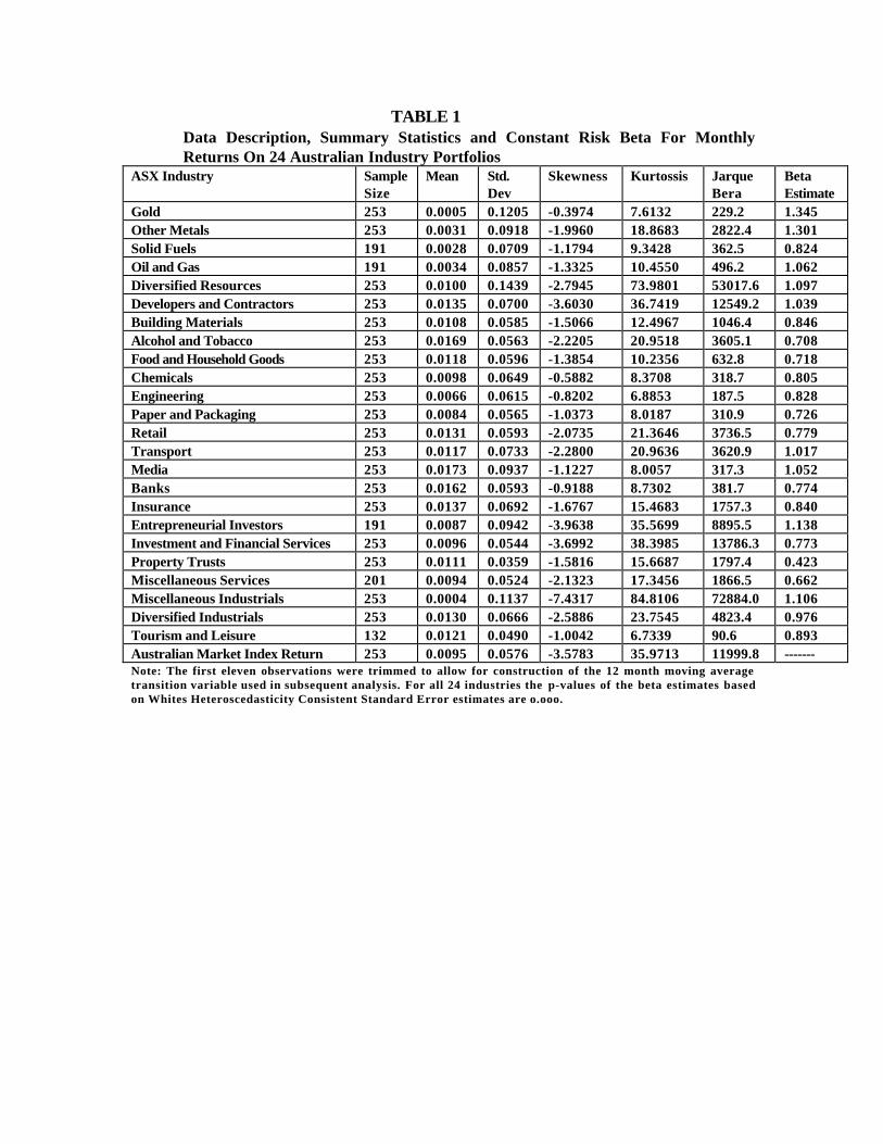
TABLE 1Data Description, Summary Statistics and Constant Risk Beta For MonthlyReturns On 24 Australian Industry Portfolios

ASX Industry SampleSize

Mean Std.Dev

Skewness Kurtossis JarqueBera

BetaEstimate

Gold 253 0.0005 0.1205 -0.3974 7.6132 229.2 1.345Other Metals 253 0.0031 0.0918 -1.9960 18.8683 2822.4 1.301Solid Fuels 191 0.0028 0.0709 -1.1794 9.3428 362.5 0.824Oil and Gas 191 0.0034 0.0857 -1.3325 10.4550 496.2 1.062Diversified Resources 253 0.0100 0.1439 -2.7945 73.9801 53017.6 1.097Developers and Contractors 253 0.0135 0.0700 -3.6030 36.7419 12549.2 1.039Building Materials 253 0.0108 0.0585 -1.5066 12.4967 1046.4 0.846Alcohol and Tobacco 253 0.0169 0.0563 -2.2205 20.9518 3605.1 0.708Food and Household Goods 253 0.0118 0.0596 -1.3854 10.2356 632.8 0.718Chemicals 253 0.0098 0.0649 -0.5882 8.3708 318.7 0.805Engineering 253 0.0066 0.0615 -0.8202 6.8853 187.5 0.828Paper and Packaging 253 0.0084 0.0565 -1.0373 8.0187 310.9 0.726Retail 253 0.0131 0.0593 -2.0735 21.3646 3736.5 0.779Transport 253 0.0117 0.0733 -2.2800 20.9636 3620.9 1.017Media 253 0.0173 0.0937 -1.1227 8.0057 317.3 1.052Banks 253 0.0162 0.0593 -0.9188 8.7302 381.7 0.774Insurance 253 0.0137 0.0692 -1.6767 15.4683 1757.3 0.840Entrepreneurial Investors 191 0.0087 0.0942 -3.9638 35.5699 8895.5 1.138Investment and Financial Services 253 0.0096 0.0544 -3.6992 38.3985 13786.3 0.773Property Trusts 253 0.0111 0.0359 -1.5816 15.6687 1797.4 0.423Miscellaneous Services 201 0.0094 0.0524 -2.1323 17.3456 1866.5 0.662Miscellaneous Industrials 253 0.0004 0.1137 -7.4317 84.8106 72884.0 1.106Diversified Industrials 253 0.0130 0.0666 -2.5886 23.7545 4823.4 0.976Tourism and Leisure 132 0.0121 0.0490 -1.0042 6.7339 90.6 0.893Australian Market Index Return 253 0.0095 0.0576 -3.5783 35.9713 11999.8 -------Note: The first eleven observations were trimmed to allow for construction of the 12 month moving averagetransition variable used in subsequent analysis. For all 24 industries the p-values of the beta estimates basedon Whites Heteroscedasticity Consistent Standard Error estimates are o.ooo.

TABLE 2Linearity Test Statistics

ASX Industry3S *

1S 1S TSAY TSAY *

Gold (XGO) 3.773(0.001)

1.358(0.256)

0.242(0.785)

0.728(0.484)

0.175(0.840)

Other Metals (XOM) 1.878(0.085)

1.855(0.138)

0.982(0.376)

1.082(0.341)

0.690(0.503)

Solid Fuels (XSF) 1.172(0.323)

0.858(0.434)

1.282(0.280)

0.892(0.412)

1.794(0.169)

Oil and Gas (XOG) 5.175(0.000)

2.753(0.044)

0.515(0.598)

2.140(0.121)

0.195(0.823)

Diversified Resources (XDR) 4.408(0.003)

3.579(0.015)

0.482(0.618)

0.838(0.434)

0.771(0.464)

Developers and Contractors (XDC) 1.043(0.398)

0.902(0.441)

0.844(0.431)

0.506(0.603)

2.438(0.090)

Building Materials (XBM) 1.247(0.283)

0.814(0.487)

0.632(0.532)

0.372(0.689)

0.307(0.736)

Alcohol and Tobacco (XAT) 2.173(0.046)

1.105(0.348)

0.048(0.953)

0.282(0.754)

0.659(0.519)

Food and Household Goods (XFH) 1.092(0.368)

1.112(0.345)

1.609(0.202)

1.925(0.148)

0.416(0.660)

Chemicals (XCE) 2.865(0.010)

5.455(0.001)

1.319(0.252)

0.217(0.805)

2.202(0.113)

Engineering (XEG) 1.402(0.214)

2.379(0.070)

2.675(0.071)

2.325(0.100)

3.101(0.047)

Paper and Packaging (XPP) 1.463(0.192)

1.988(0.116)

0.502(0.606)

0.533(0.587)

0.405(0.667)

Retail (XRE) 0.686(0.661)

0.487(0.692)

0.467(0.628)

1.360(0.259)

0.710(0.493)

Transport (XTP) 3.724(0.002)

7.764(0.000)

1.377(0.254)

1.531(0.219)

1.470(0.232)

Media (XME) 0.967(0.448)

1.563(0.199)

1.436(0.240)

1.825(0.163)

1.114(0.330)

Banks (XBF) 0.498(0.810)

0.217(0.805)

0.145(0.933)

0.859(0.425)

0.200(0.819)

Insurance (XIN) 15.843(0.000)

3.497(0.016)

4.447(0.013)

4.955(0.008)

3.275(0.040)

Entrepreneurial Investors (XEI) 1.700(0.123)

1.855(0.139)

2.720(0.069)

2.410(0.093)

4.326(0.015)

Investment and Financial Services (XIF) 1.709(0.119)

0.925(0.429)

1.009(0.366)

0.088(0.916)

6.102(0.003)

Property Trusts (XPT) 0.788(0.580)

0.063(0.979)

0.091(0.913)

0.049(0.952)

0.400(0.671)

Miscellaneous Services (XMS) 4.080(0.001)

1.054(0.370)

0.415(0.661)

1.060(0.349)

0.448(0.639)

Miscellaneous Industrials (XMI) 3.206(0.005)

2.262(0.082)

0.345(0.709)

1.512(0.216)

0.140(0.869)

Diversified Industrials (XDI) 2.784(0.012)

0.260(0.854)

0.349(0.705)

0.364(0.695)

1.247(0.289)

Tourism and Leisure (XTU) 3.135(0.007)

0.319(0.812)

0.378(0.686)

0.425(0.655)

0.572(0.566)

Note: S S1 1, * and S 3are respectively the Luukkonen first order, augmented first order and third order F-versions of the

Lagrange Multiplier type tests of nonlinearity. TSAY and TSAY * are the Tsay F-statistics for the data sorted in ascending

and descending order respectively. P-values are in parentheses next to the calculated values of the statistics. The codenames, given by SIRCA, are in parentheses next to the unabbreviated descriptions of the industries.

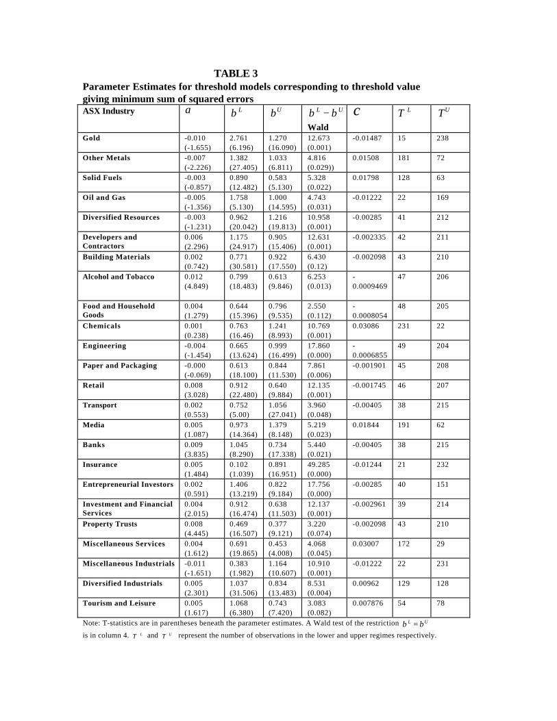
TABLE 3Parameter Estimates for threshold models corresponding to threshold valuegiving minimum sum of squared errorsASX Industry α β L βU β βL U−

Wald

c LT TU

Gold -0.010(-1.655)

2.761(6.196)

1.270(16.090)

12.673(0.001)

-0.01487 15 238

Other Metals -0.007(-2.226)

1.382(27.405)

1.033(6.811)

4.816(0.029))

0.01508 181 72

Solid Fuels -0.003(-0.857)

0.890(12.482)

0.583(5.130)

5.328(0.022)

0.01798 128 63

Oil and Gas -0.005(-1.356)

1.758(5.130)

1.000(14.595)

4.743(0.031)

-0.01222 22 169

Diversified Resources -0.003(-1.231)

0.962(20.042)

1.216(19.813)

10.958(0.001)

-0.00285 41 212

Developers andContractors

0.006(2.296)

1.175(24.917)

0.905(15.406)

12.631(0.001)

-0.002335 42 211

Building Materials 0.002(0.742)

0.771(30.581)

0.922(17.550)

6.430(0.12)

-0.002098 43 210

Alcohol and Tobacco 0.012(4.849)

0.799(18.483)

0.613(9.846)

6.253(0.013)

-0.0009469

47 206

Food and HouseholdGoods

0.004(1.279)

0.644(15.396)

0.796(9.535)

2.550(0.112)

-0.0008054

48 205

Chemicals 0.001(0.238)

0.763(16.46)

1.241(8.993)

10.769(0.001)

0.03086 231 22

Engineering -0.004(-1.454)

0.665(13.624)

0.999(16.499)

17.860(0.000)

-0.0006855

49 204

Paper and Packaging -0.000(-0.069)

0.613(18.100)

0.844(11.530)

7.861(0.006)

-0.001901 45 208

Retail 0.008(3.028)

0.912(22.480)

0.640(9.884)

12.135(0.001)

-0.001745 46 207

Transport 0.002(0.553)

0.752(5.00)

1.056(27.041)

3.960(0.048)

-0.00405 38 215

Media 0.005(1.087)

0.973(14.364)

1.379(8.148)

5.219(0.023)

0.01844 191 62

Banks 0.009(3.835)

1.045(8.290)

0.734(17.338)

5.440(0.021)

-0.00405 38 215

Insurance 0.005(1.484)

0.102(1.039)

0.891(16.951)

49.285(0.000)

-0.01244 21 232

Entrepreneurial Investors 0.002(0.591)

1.406(13.219)

0.822(9.184)

17.756(0.000)

-0.00285 40 151

Investment and FinancialServices

0.004(2.015)

0.912(16.474)

0.638(11.503)

12.137(0.001)

-0.002961 39 214

Property Trusts 0.008(4.445)

0.469(16.507)

0.377(9.121)

3.220(0.074)

-0.002098 43 210

Miscellaneous Services 0.004(1.612)

0.691(19.865)

0.453(4.008)

4.068(0.045)

0.03007 172 29

Miscellaneous Industrials -0.011(-1.651)

0.383(1.982)

1.164(10.607)

10.910(0.001)

-0.01222 22 231

Diversified Industrials 0.005(2.301)

1.037(31.506)

0.834(13.483)

8.531(0.004)

0.00962 129 128

Tourism and Leisure 0.005(1.617)

1.068(6.380)

0.743(7.420)

3.083(0.082)

0.007876 54 78

Note: T-statistics are in parentheses beneath the parameter estimates. A Wald test of the restriction β βL U=is in column 4. T L and T U represent the number of observations in the lower and upper regimes respectively.

.360

.364

.368

.372

.376

.380

-.02 -.01 .00 .01 .02 .03 .04

RSTAR

XR

E

XRE

-0.0017

Figure 3

.258

.259

.260

.261

.262

.263

-.02 -.01 .00 .01 .02 .03 .04

XBM

-0.0021

Figures 1 is a graph of the return on the market portfolio with horizontal lines at zero and the median of the return on the

market. Figure 2 is a graph of the 12 month moving average of the return on the market with typical threshold estimate

superimposed as the horizontal line. Figure 3 is the graphs of the DBM sum of squared errors against corresponding threshold

values, for the two typical industries, Retail and Building Materials, for which linearity was not rejected.

-0.6

-0.4

-0.2

0.0

0.2

82 84 86 88 90 92 94 96 98 00

Return on Market Median of return on Market Zero

Figure 1

-0.04

-0.02

0.00

0.02

0.04

0.06

82 84 86 88 90 92 94 96 98 00

12 month moving average Threshold of -0.002

Figure 2