1

A Multi-Objective Decision Framework for Credit Portfolio

Management

Juan C. Moreno-Paredes / School of Management University of Southampton. Highfield Campus

Southampton United Kingdom SO17 1BJ. E-mail: J.C.Moreno-Paredes@soton.ac.uk

Christophe Mues / School of Management University of Southampton. Highfield Campus

Southampton United Kingdom SO17 1BJ. E-mail: C.Mues@soton.ac.uk

Lyn C. Thomas / School of Management University of Southampton. Highfield Campus

Southampton United Kingdom SO17 1BJ. E-mail: L.Thomas@soton.ac.uk

Abstract

In this paper a framework is proposed which is meant to support the portfolio

optimisation problem, i.e. how to allocate bank’s resources across various sectors of

loans in order to maximise profitability and minimise risk. The framework enables

analysts to select an appropriate combination of performance measures and use a

multiple-objective optimisation technique to increase portfolio performance. A small

case study where the framework is applied shows how the risk and return can be

improved whilst simultaneously diversifying the credit portfolio.

Keywords: Credit Risk Management framework, Credit Portfolio Optimisation, Multi-

Objective Optimisation, Credit VaR, Credit Expected Shortfall.

1. Introduction

Since the Basel I and II accords (BCBS, 2005) established guidance for internal

models, the use of a variety of mathematical models and techniques in the financial

sector has become standard practice. Data driven models are widely used in the

financial sector to estimate the different levels of credit risk associated with obligors

involved in a credit transaction.

There is significant literature about techniques and methods to estimate credit risk at

the individual loan level (e.g. Thomas (2009); Thomas, Edelman and Crook (2004);

Thomas, Edelman and Crook (2002)).

On the other hand, further research is emerging to assess the overall risk of credit

portfolios (i.e. groups of loans) as interaction among the assets arises when they are

combined in the portfolio. For example, Cespedes (2002) shows how the correlation of

defaults can produce bigger losses in a credit portfolio. Additionally, phenomena like

2

concentration, correlation and contagion make the measurement of the risk of losses in

a credit portfolio more complex (Herbertsson (2011); Lütkebohmert (2009)).

An added complication with the credit portfolios of commercial and retail banks in

particular is that they are built of non-liquid assets like private loans. For that reason,

the quantitative analysis of such portfolios is challenging. For instance, for corporate

loans and bonds, risk metrics such as probability of default and loss given default are

constantly updated by the rating agencies, in contrast with private loans for whom no

such public information is found. Therefore, strategies aiming to improve the

performance of a credit portfolio are often made based on expert judgement. (Thomas

(2009); Lütkebohmert (2009); Schlottmann et al. (2010)).

A survey of approaches to optimise portfolios has to start with the Novel laureate

Markowitz (1952) who established the theoretical basis for portfolio analysis. Markowitz’

approach however cannot be applied directly to credit portfolios as the distribution of

the risk of losses does not follow a normal distribution (Cespedes, 2002). Also, the risk

in a credit portfolio is not adequately represented by one single risk measure. For that

reason, Zopounidis and Doumpos (2002) suggested a multi-objective approach to

integrate different risk metrics; however, they do not present details of how these

different metrics have to be calculated. Schlottmann and Seese (2004) present a hybrid

version of multi-objective evolutionary algorithms to optimise credit portfolios in

combination with CreditRisk+®, an actuarial model developed by Credit Suisse

Financial Products (CSFP, 1997) to calculate the risk of losses. They use a binary

encoding for modelling the decision variables which could be inefficient though to

optimise large portfolios. Additionally, this encoding is focused at the individual loan

level, whereas usually the main decisions in financial institutions are taken at a more

aggregate sector/segment level. Also, risk metrics such as concentration and

correlation among the sectors, are not yet taken into account as the methodology is

illustrated using a portfolio of one sector only.

Therefore, one of the main contributions in this paper is to propose a practical

framework where the risk metrics are explicitly disclosed and integrated using a Multi-

Objective Algorithm to support the credit portfolio optimisation process. The framework

integrates the profitability and risk perspectives; whereas the first perspective focuses

on finding opportunities to increase the portfolio’s return, the second perspective aims

to reduce the expected and unexpected losses and concentration risk of the portfolio.

3

We illustrate the suggested approach for a credit portfolio belonging to a financial

institution, thereby considering multi-sector and sector correlations. We also specify the

kind of data that would be needed for financial institutions to implement the approach.

This paper is organised as follows: In section 2, the profitability and risk perspective of

credit risk management are presented. Section 3 describes the process of modelling

the credit portfolio; in this section, the notation to represent the credit portfolio problem

and the measures associated with credit portfolio performance are established. Section

4 discusses the methods that are used to compute the solutions of the credit portfolio

optimisation problem and outlines the data required to perform this process. In section

5, the proposed framework is presented. In section 6, a practical case is presented in

order to illustrate how the framework operates. Finally, in section 7, conclusions are

drawn.

2. Perspectives of the credit portfolio management problem.

Credit portfolios from retail and commercial banks are characterised by a collection of

loans which are usually not liquid and therefore they are not easily sold to a third party

in the marketplace, unless they are properly packaged into “special purpose vehicles”

(SPV) (Thomas (2009)).

Each loan is a contract between a financial institution (FI) and individuals (called

obligors) where the FI lends an amount of money to the obligor who agrees to repay

later on. In some cases the obligors have to put some assets up as a guarantee

(collateral). In case the obligor defaults on its payments, the FI is able to repossess this

collateral in order to recover at least part of the lent money.

Credit portfolio management implies finding effective and efficient solutions as to how

to reorganise the portfolio in order to improve its profitability and reduce its total risk.

We refer to these (often competing) criteria as the profitability and risk perspective of

credit portfolio management.

Under the profitability perspective, the main objective of the portfolio managers is to

spot investment opportunities. Therefore elements such as return, profitability, pricing

and planning are key factors.

On the other hand, under the risk perspective, the portfolio managers have to identify

and anticipate real and potential losses as well as assess and quantify them; setting

4

exposure limits and capital reserves to mitigate and cover those potential losses are the

main elements to be considered (Thomas (2009); Van Gestel and Baesens (2009)).

In Figure 1, a graphical representation of these two perspectives is presented.

Figure 1 Perspectives and interactions in a credit portfolio.

Summing up, in order to further develop the risk and profitability perspectives it is

necessary to address the following questions:

a) What are the metrics associated with the performance of a credit portfolio?

b) What data should be used to calculate these metrics?

c) How is it possible to improve the performance of a credit portfolio reflecting

effectiveness and efficiency, i.e. higher returns and lower risk?

In the following sections, a framework is developed to address these questions.

3. Credit portfolio modelling

In this section, the notation to represent the credit portfolio optimisation problem and

the measures associated with credit portfolio performance are presented.

3.1. Credit portfolio definition

Following the definition of Markowitz (1952) according to which a portfolio can be

represented as a collection of assets that an investor can purchase using a predefined

amount of money, we define a credit portfolio as a set of credit operations (Assets). A

Soundness system of acredit portfolio risk management

(Risk perspective)

Soundness system of acredit portfolio risk management

(Profitability perspective)

S

E

G

M

E

N

T

S

/

S

E

C

T

O

R

S

Commercial

Manufacture

Corporate

Retail

Unsecure Loans

C

O

L

L

A

T

E

R

A

L

S

Land / Real Estate

Inventories and

Receivables

Cash

Marketable financial

instruments

Other Guaranties

and

Collaterals

Exposures Collateral

Loss Given Default (LGD)

Exposure Risk (EAD)

DefaultRisk (PD)

PortfolioStructure

(x1,…,xn)% of loans in n

sectors / segments

ConcentrationRisk

Stress testing& Limits

Scenario planning

Pricing

PotentialLosses

ExpectedReturns

Provisions and reserves

Regulatorycapital

RAROC &Profitability

5

credit operation is established when a FI (Investor) lends a predefined amount of

money (Exposure) to a counterparty (Obligor) that is willing to repay over a certain

period of time and in most of the cases paying an interest rate.

The FIs make strategic planning on their portfolios analysing not each individual credit

operation, but sets of them, grouped by segments or sectors such as real estate,

manufacturing, credit cards, agriculture and car loans.

Stratifying the portfolio into sectors makes it possible to analyse the risk due to

common factors, called systematic factors. The systematic factors are the underlying

common elements that could affect one significant part of the portfolio. For example, if

the real estate sector has performed badly in the economy recently, all the investments

in this sector could also be affected.

On the other hand, some portfolio metrics, as shown below, are specific to each loan in

the portfolio. For that reason it is important to consider two “levels” when a credit

portfolio is studied, i.e. the loan level and the sector level. The following notation is

used to represent these two levels:

Let be the proportion of money invested in loan in sector . The proportion

invested in sector is given by:

∑

Eq. 1

where : the number of loans in sector .

Definition 3.1: A credit portfolio can be defined as a vector , where is

the proportion of the portfolio invested in the sector ; ; ∑ and is the

number of sectors.

3.2. Credit portfolio performance metrics

The performance of a credit portfolio can be summarised by two main elements: the

returns produced by the repayments of the performing loans and the losses caused by

the default of loans. Hence, the default event is the main trigger that could produce

losses in the credit portfolio.

6

Definition 3.2: Let the random variable represent the default of a loan; hence

implies loan in sector defaults, or otherwise. The probability of default is

the associated probability of this event.

Definition 3.3: The risk of exposure or exposure at default ( ) is the book value of

the loans associated to loan in sector when the loan defaults. The EAD could be a

stochastic value, particularly when loans are credit lines or credit cards. BCBS (2005

parg. 311-315 and parg. 474 - 478) establishes the conditions that FIs should follow to

estimate EAD values. In this paper, the EADs are treated as deterministic values.

Definition 3.4: The severity of the loss ( ) is the portion of the value of the loans

that is lost after the loan defaults. The severity of the loss is also stochastic and its

expected value is the loss given default ( ) (Bluhm, Overbeck and Wagner, 2003).

BCBS (2005 parag. 286 - 307) details the conditions to work out the LGDs in a credit

portfolio.

Using these previous metrics, the return for a particular loan can be modelled:

( ) ( )

Eq. 2

where is the annual interest rate associated with a particular loan, net of cost of

funding and expenses.

Given that is the probability of default of a particular loan and its loss given

default, the expected return can be expressed as follows:

( ) ( )

Eq. 3

It should be noted that Eq. 3 assumes independency between the LGDs and PDs.

Comments about the implications of this assumption are made in Bluhm, Overbeck and

Wagner (2003 pg 28); Allen and Saunders (2004); Miu and Ozdemir (2006).

Then the expected return of a credit portfolio is represented by:

( ) ∑∑ ( )

Eq. 4

7

On the other hand, the associated loss of a particular loan is given by:

( )

Eq. 5

Thus, the expected loss is:

( )

Eq. 6

Similarly, the expected loss (EL) in a credit portfolio is given by:

( ) ∑∑

Eq. 7

EL only captures potential losses based on the historical default experience of each FI.

Hence, holding reserves to absorb only expected losses are not enough for FIs (Bluhm,

Overbeck and Wagner, 2003). Therefore, metrics that estimate unexpected losses help

FIs set aside enough capital to cover additional losses.

Vasicek (2002) proposes Value at Risk (VaR) as a measure for unexpected losses in a

portfolio. VaR is a one-factor extension of the Merton model and is used in BCBS

(2005) to set the minimum capital requirement. This is the value so that the chance of

getting a greater loss is no more than for a prespecified ( ).

Let ( ) be the loss associated with the portfolio . For a fixed ( the credit

portfolio VaR at level can be defined as follows:

( ) ( ( )) Eq. 8

where is the supremum function.

Artzner et al. (1999) propose a framework with the properties that a risk measure

should have in order to be mathematically coherent. Even though VaR is widely used in

the financial sector and it is supported by BCBS (2005), this metric is not a coherent

risk measure as it fails in the subadditivity property and it is law invariant (Tasche,

2002).

8

The lack of subadditivity makes it complex to analyse the risk contribution of a portion

of the portfolio (Tasche (2002)). And because VaR is law invariant it can produce the

same result for portfolios with light and fat tails (see e.g. Embrechts, Klüppelberg and

Mikosch (1997)). For that reason a more robust metric should be considered.

In order to tackle the problems of the VaR measure, Acerbi and Tasche (2002) propose

the Expected Shortfall (also known as Conditional VaR or CVaR) as a risk metric to

estimate the unexpected losses in the portfolio. The definition of CVaR is presented as

follows:

( )

( )∫ ( )

Eq. 9

Definition 3.5. Economic Capital (EC) is the amount of capital that each FI estimates

by itself in order to cover its potential losses. In this paper the EC is given by:

( ) ( ) ( ) Eq. 10

Where ( ) is the unexpected losses, calculated using one of the mentioned

methods, e.g. VaR or CVaR, at level, of the portfolio .

Definition 3.7. The Risk-adjusted Return on Capital is a metric that combines the

portfolio’s return and its EC, as represented in Eq. 11.

( ) ( ) ( ) Eq. 11

The ( ) is economic capital at level of the portfolio .

Another element that should be taken into consideration when a credit portfolio is

analysed is the concentration risk. Concentration risk arises due to the uneven

distribution of the loans in the different sectors. Lütkebohmert (2009) makes a survey of

the different methods to calculate concentration risk, classifying them into two groups:

ad hoc methods and model-based methods. She also presents several properties that

a concentration index for credit portfolios should have in order to be mathematically

consistent.

9

One of the ad hoc methods presented by Lütkebohmert (2009) is the Herfindahl-

Hirschman (HHI index). Becker and Düllmann (2004) prove that HHI fulfils the

concentration index properties.

In this paper, the HHI is adapted to measure concentration in the sectors as follows:

( ) ∑( )

Eq. 12

Hence, portfolios that are highly concentrated in a few sectors will produce a HHI

nearer to 1, whereas more balanced portfolios will produce a HHI nearer to 0.

3.3. Integrating risk metrics to optimise the credit portfolio.

For improving the performance of a credit portfolio in terms of effectiveness and

efficiency, i.e. in order to find higher returns and lower risk, it is necessary to integrate

the different risk metrics and represent the problem in the form of an optimisation

program.

RAROC in particular combines the expected return and the EC. However as it is

argued in previous work (Moreno-Paredes (2009)), optimising the credit portfolio using

RAROC as the objective function can be misleading as it cannot guarantee effective

and efficient solutions; i.e. some solutions obtained using RAROC as the sole goal

metric may consist of portfolios with higher risk than the original ones.

Similarly, there are important efforts in the literature to develop mathematical models

capable of integrating concentration metrics into the EC calculations. Particularly,

Lütkebohmert (2009 p 72-73) argues that ad hoc methods like the HHI could be

unsuitable as the outcomes they produce cannot be related directly to the EC

estimation. For that reason, she suggests using model-based methods such as

Granularity Adjustment, Semi Asymptotic approach and methods based on Saddle-

Point Approximation. Details of these methodologies can be found in Gordy (2004);

Emmer and Tasche (2004) and Gordy (2002), respectively.

However, integrated models like the ones listed above could be complex to implement

for credit portfolios of commercial and retail banks, as these credit portfolios are mainly

composed of low liquidity assets such as private loans; for that reason insufficient

information is available to fulfil the requirements of these models.

10

An integration approach whereby it is possible to preserve each metric is presented by

Zopounidis and Doumpos (2002). They suggest Multi-Objective Optimisation

programming whereby each metric is maximised or minimised simultaneously. A similar

approach is developed by Schlottmann, Mitschele and Seese (2005) when they are

attempting to combine different risk measures to model credit risk, market risk and

operational risk in FIs.

The main advantage of the Multi-Objective framework is the flexibility that it gives to

include different metrics in the modelling process. However, one needs to clearly define

the rules and interactions between the solutions, in particular the dominancy criteria.

These are defined in the following sections.

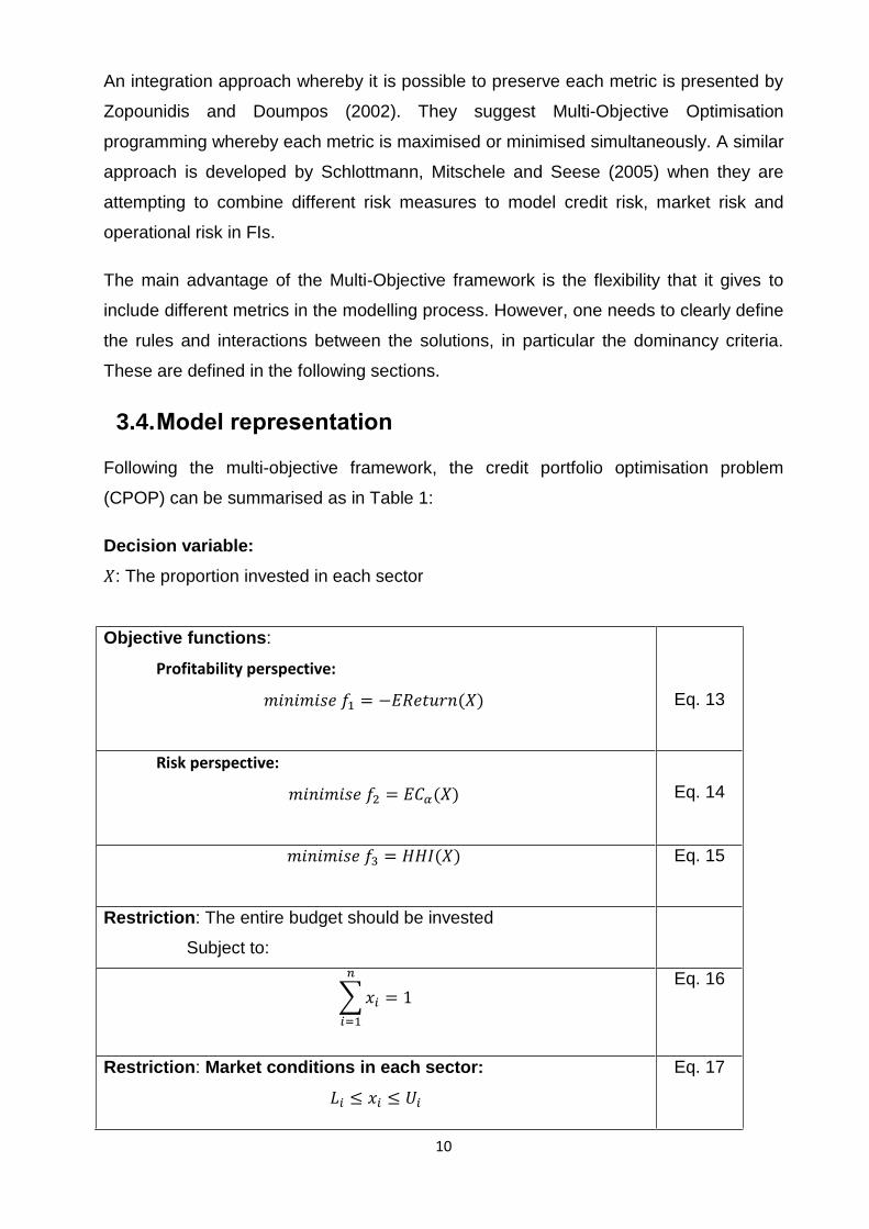
3.4. Model representation

Following the multi-objective framework, the credit portfolio optimisation problem

(CPOP) can be summarised as in Table 1:

Decision variable:

: The proportion invested in each sector

Objective functions:

Profitability perspective:

( )

Eq. 13

Risk perspective:

( )

Eq. 14

( )

Eq. 15

Restriction: The entire budget should be invested

Subject to:

∑

Eq. 16

Restriction: Market conditions in each sector:

Eq. 17

11

where represents the no short sell allowance restriction

and is the sector maximum saturation.

Table 1. The credit portfolio optimisation problem (CPOP).

The Market conditions in Eq 17 are modelling the minimum and maximum exposure in

each sector. These are related to elements such as regulatory restrictions1 or market

saturation. This information should be set up by the FI’s managerial team.

The credit portfolio optimisation problem has the following assumptions:

1. The loan’s participation , within the sector, remains constant in the short

term2.

2. The , and return rates remain constant during a period of time3.

3. Each loan can only belong to one sector4.

The Multi-Objective framework makes it possible to combine different metrics, without

the challenging effort of integrating all into a single optimisation criterion. Also its

flexibility allows including more or other metrics.

4. Methods to compute the solutions

Generating solutions that solve the CPOP (Table 1) can be a challenge as the

computation of the unexpected losses is not straightforward; this is because it is not

obvious how to model the distribution of the losses of a credit portfolio. Therefore

computational methods are required to tackle this problem.

4.1. Methods to compute Unexpected Losses.

In the case of credit portfolios, the assumption of normality in the distribution of losses

would be misleading as the correlation between defaults can produce higher losses.

These distributions are usually characterised by having big kurtosis (fat tails) (see

Cespedes (2002)).

1 Some FIs want to maintain a minimal investment in strategic sectors. Also, in some countries regulators can

request a minimum participation of the portfolio in a particular sector such as agriculture. 2 It can be assumed that these proportions do not change drastically in the short term.

3 Usually the FIs re-calculate these values periodically to keep the portfolio data up-to-date.

4 In this case the FIs associate a loan to its most related sector.

12

Jorion (2009) and also Thomas (2009) produce a survey of the most popular methods

in the banking sector to estimate the distribution of losses in a credit portfolio.

One such method is CreditRisk+® proposed by Credit Suisse Financial Products

(CSFP, 1997). This approach considers the distributions of defaults and of the severity

of the losses to build the distribution function of losses. The distribution of the number

of defaults is modelled using the Poisson distribution, based on the assumption that the

PDs are small enough and independent among the loans. CreditRisk+® splits the

portfolio into sectors where the loans may have some systematic risk factors in

common. Initially, in CSFP (1997), the sectors are considered independent. Bürgisser

et al. (1999), Han and Kang (2008) and Fisher and Dietz (2011) present improved

versions of CreditRisk+® where it is possible to use correlated sectors.

Some advantages that CreditRisk+® has when compared with other methods are: it

produces deterministic solutions; therefore, random variations in the solutions,

introduced by methods based on simulation, are avoided. Also, this method is well

documented in the literature. For those reasons, CreditRisk+® is used in this paper in

order to illustrate how the framework operates. However, it is important to note that the

proposed framework is able to use any alternative method to estimate the unexpected

losses.

4.2. Methods to solve the CPOP.

As it is mentioned above, the CPOP is modelled under the Multi-Objective Optimisation

Problems (MOOP) approach. In general, solutions of MOOPs are characterised by the

following properties. Firstly, objectives are usually in conflict with each other, i.e. better

returns often imply higher risk. Secondly, the dominancy of the solutions; a possible

solution is called dominated by , if is better in all objectives than . In contrast is

called a non-dominated solution when there is no solution such that dominates .

Thirdly, there is often more than one possible non-dominated optimal solution. Finally,

all optimal solutions are located in a set called the Pareto-Optimal Front (also referred

to in the literature as the Efficient Front; refers to Markowitz (1952)). Figure 2 illustrates

these characteristics. Here the grey area represents the space of valid solutions for the

CPOP and a, b and c are three specific solutions to the problem.

13

Figure 2 Efficient Front in MOOP.

Note that solution c is not an optimal solution, because it is dominated by a and b.

Particularly, for the CPOP the dominancy criteria can be defined as follows (see Deb

(2008)):

Definition 4.1. Let be a solution of the CPOP. dominates when at least one of

these conditions are true:

( ) ( ) ( ) ( ) ( ) ( )

( ) ( ) ( ) ( ) ( ) ( )

( ) ( ) ( ) ( ) ( ) ( ).

Deb (2008 pg 28) explains in detail how dominancy plays a major role in the multi-

objective optimisation.

Generic optimisation methods called meta heuristics can be suitable for solving the

CPOP as conventional methods could have difficulties coping with the complexity

involved in the calculus of the objective functions, especially for the EC criterion. In

Moreno-Paredes (2009) it is shown how a conventional optimisation method such as

the Conjugate Gradient algorithm fails to solve this class of problems.

A Multi-Objective Evolutionary Algorithm (MOEA) is one of the meta-heuristics that has

been used successfully to solve these problems (Schlottmann and Seese (2004);

Branke et al. (2009); Moreno-Paredes (2009)). Deb (2008) presents a comprehensive

survey of these methods.

14

4.3. Data availability

In order to implement this framework, the FIs, particularly commercial and retail banks,

must have the following set of data for each loan: EAD, PD, LGD and Sector, as

illustrated in Table 2. For the computation of PDs and LGDs, the FIs have to collect

information of the default and recovery rates over a period of time long enough to

reflect economic downturn in these values (BCBS, 2005).

Loan ID EAD PD LGD Sector

O0001 £ 5,000.00 0.02 50% A

O0002 £ 3,000.00 0.07 80% B

O0003 £ 2,500.00 0.01 30% A

O0004 £ 6,000.00 0.07 40% C

Table 2 EAD, PD, and LGD; example.

Also, they have to calculate the Pearson correlation of the default rates among the

sectors over a period of time (see Table 3 for an example table).

Sector A B C

A

1.00

0.30

0.20

B

0.30

1.00 -

0.75

C

0.20 -

0.75

1.00

Table 3 Sector correlations; example.

Furthermore, Market conditions for each sector must be specified (see Table 4).

Sector LB UB

A 0.01 0.10

B 0.02 0.30

C 0.06 0.20

Table 4 Market conditions; example.

The default volatilities of the sectors are defined as the standard deviation of the

number of defaults in each sector divided by the average of the number of defaults in

each sector. Additionally, the returns of the portfolio are given by the annual interest

15

rates, less the cost of funding annually, commissions and fees incurred. The default

volatilities and the annual net returns are illustrated in Table 5.

Sector Default-

Volatilities Returns

A 0.02 1%

B 0.01 2%

C 0.03 3.5%

Table 5 Sector conditions; example.

These data are the inputs required to calculate the unexpected losses via

CreditRisk+®. Further details are given in section 6.

5. Framework outline

In Figure 3, the framework proposed in this paper is summarised.

Figure 3 Framework outline.

Inputs: Portfolio Risk

Indicators:

• PD, EAD, LGD

• Correlation

• PD volatilities

• Returns

• Market conditions

Output:

Strategies to

improve the

portfolio

Calculate the Portfolio

Performance Measures

(Return, EL, EC, HHI, etc.)

Solve the CPOP

Using MOEA

Populate the

model for the

CPOP

16

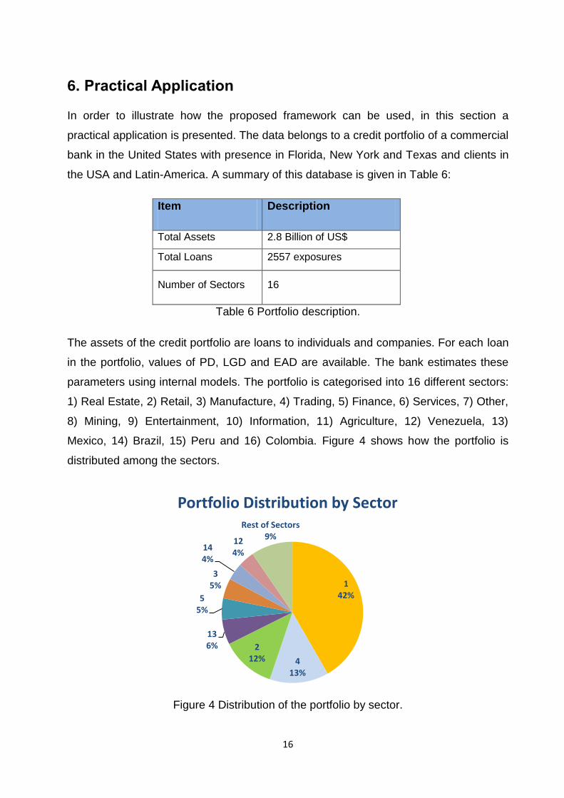
6. Practical Application

In order to illustrate how the proposed framework can be used, in this section a

practical application is presented. The data belongs to a credit portfolio of a commercial

bank in the United States with presence in Florida, New York and Texas and clients in

the USA and Latin-America. A summary of this database is given in Table 6:

Item Description

Total Assets 2.8 Billion of US$

Total Loans 2557 exposures

Number of Sectors 16

Table 6 Portfolio description.

The assets of the credit portfolio are loans to individuals and companies. For each loan

in the portfolio, values of PD, LGD and EAD are available. The bank estimates these

parameters using internal models. The portfolio is categorised into 16 different sectors:

1) Real Estate, 2) Retail, 3) Manufacture, 4) Trading, 5) Finance, 6) Services, 7) Other,

8) Mining, 9) Entertainment, 10) Information, 11) Agriculture, 12) Venezuela, 13)

Mexico, 14) Brazil, 15) Peru and 16) Colombia. Figure 4 shows how the portfolio is

distributed among the sectors.

Figure 4 Distribution of the portfolio by sector.

142%

413%

212%

136%

55%

35%

144%

124%

Rest of Sectors9%

Portfolio Distribution by Sector

17

The sectors of the portfolio are not independent; the inter-sector correlation matrix

between the sectors is presented in Table 7.

Sect

or 1

Sect

or 2

Sect

or 3

Sect

or 4

Sect

or 5

Sect

or 6

Sect

or 7

Sect

or 8

Sect

or 9

Sect

or 1

0

Sect

or 1

1

Sect

or 1

2

Sect

or 1

3

Sect

or 1

4

Sect

or 1

5

Sect

or 1

6

Sector 1 1.00 0.41 0.54 0.84 -0.05 0.25 0.41 0.96 0.12 0.61 0.19 0.09 0.28 0.27 0.13 0.01

Sector 2 0.41 1.00 0.34 0.41 -0.16 0.10 0.99 0.39 0.82 0.00 0.07 0.09 -0.19 -0.04 0.12 0.30

Sector 3 0.54 0.34 1.00 0.42 0.10 0.53 0.34 0.60 -0.02 0.34 0.33 -0.05 0.34 0.41 0.42 0.16

Sector 4 0.84 0.41 0.42 1.00 -0.01 0.02 0.41 0.83 0.25 0.42 0.33 -0.01 0.45 -0.08 -0.12 -0.15

Sector 5 -0.05 -0.16 0.10 -0.01 1.00 0.40 -0.16 -0.05 -0.08 0.01 0.47 -0.16 0.45 -0.15 -0.25 -0.38

Sector 6 0.25 0.10 0.53 0.02 0.40 1.00 0.10 0.24 -0.06 0.35 0.31 -0.21 0.02 0.15 0.19 -0.04

Sector 7 0.41 0.99 0.34 0.41 -0.16 0.10 1.00 0.39 0.82 0.00 0.07 0.09 -0.19 -0.04 0.12 0.30

Sector 8 0.96 0.39 0.60 0.83 -0.05 0.24 0.39 1.00 0.02 0.51 0.18 -0.07 0.27 0.28 0.19 0.04

Sector 9 0.12 0.82 -0.02 0.25 -0.08 -0.06 0.82 0.02 1.00 -0.10 0.11 0.15 -0.17 -0.33 -0.17 -0.01

Sector 10 0.61 0.00 0.34 0.42 0.01 0.35 0.00 0.51 -0.10 1.00 -0.09 0.11 0.21 -0.04 -0.23 -0.45

Sector 11 0.19 0.07 0.33 0.33 0.47 0.31 0.07 0.18 0.11 -0.09 1.00 -0.19 0.67 -0.03 0.09 -0.10

Sector 12 0.09 0.09 -0.05 -0.01 -0.16 -0.21 0.09 -0.07 0.15 0.11 -0.19 1.00 0.16 0.26 0.03 0.40

Sector 13 0.28 -0.19 0.34 0.45 0.45 0.02 -0.19 0.27 -0.17 0.21 0.67 0.16 1.00 -0.06 -0.20 -0.21

Sector 14 0.27 -0.04 0.41 -0.08 -0.15 0.15 -0.04 0.28 -0.33 -0.04 -0.03 0.26 -0.06 1.00 0.79 0.60

Sector 15 0.13 0.12 0.42 -0.12 -0.25 0.19 0.12 0.19 -0.17 -0.23 0.09 0.03 -0.20 0.79 1.00 0.57

Sector 16 0.01 0.30 0.16 -0.15 -0.38 -0.04 0.30 0.04 -0.01 -0.45 -0.10 0.40 -0.21 0.60 0.57 1.00

Table 7 Correlation matrix among the sectors.

The volatilities and the annual net returns for each sector of the portfolio are given by

Table 8:

Sector Volatilities Returns

1 0.22 1.91%

2 0.17 0.41%

3 0.33 -0.72%

4 0.22 0.29%

5 0.06 -1.77%

6 0.15 0.15%

7 0.17 0.39%

8 0.35 0.06%

9 0.17 -0.83%

10 0.41 -1.46%

11 0.89 0.11%

12 0.73 0.87%

13 0.32 0.78%

14 0.21 -0.83%

15 0.36 0.12%

16 0.25 -0.34%

Table 8 Volatilities and annual returns by sector.

The Market Conditions (L and U) were calculated by dividing the minimum and

maximum exposure that the bank is willing to invest in this sector over the total

exposure of the credit portfolio, respectively. The resulting market conditions are

presented in Table 9.

18

Sector L U

1 0.000016819% 100%

2 0.000046288% 100%

3 0.000002066% 100%

4 0.000007322% 100%

5 0.000001269% 100%

6 0.000003842% 100%

7 0.000001414% 100%

8 0.000000036% 100%

9 0.000000580% 100%

10 0.000000217% 100%

11 0.000000072% 100%

12 0.000010729% 100%

13 0.000000761% 100%

14 0.000000399% 100%

15 0.000000399% 100%

16 0.000000471% 100%

Table 9 Market conditions.

In order to compute the VaR and CVaR, the version of CreditRisk+® by Haaf, Rieß and

Schoenmakers (2004) is used in combination with the Bürgisser et al. (1999) approach.

By integrating both versions it is possible to have a numerically stable version of

CreditRisk+® which also allows for calculating the CVaR and dealing with correlated

sectors.

To solve the associated CPOP (see Table 1), Non-Dominated Sorting Genetic

Algorithm type II (NSGA II), a type of MOEA developed by Deb and Goel (2001) is

used. The initial settings and stop conditions of this algorithm are the same as specified

by Moreno-Paredes (2009); however these parameters settings would have to be

adjusted for other credit portfolios. The problem of parameter selection goes beyond

the scope of this paper.

Parameter Value

Pc: Probability of Crossover 0.9

Pm: Probability of mutation 0.9

Max number of generation 500

Initial Population Random

initialization

Number of max generation 500

Number of runs 50

Table 10 MOEA initialisation parameters.

19

The numerical representation and genetic procedures in the NSGA II algorithm were

implemented using the approaches in Moreno-Paredes (2009) and Dinovella and

Moreno-Paredes (2005).

A graphical representation of the solutions produced by the MOEA is shown in Figure

5. Here, the values of the portfolio metrics are plotted for each solution, the colours

representing the RAROC.

Figure 5 Solutions from the MOEA.

In Table 11, we decide to select the solution with the higher RAROC and label it as

“Best Solution”, but this selection is arbitrary and it is made just to show how the

optimisation process helps to improve the performance of the credit portfolio.

Initial

Portfolio

Best

Solution

Improvement

(%)

Average

Solution

Average

Improvement

(%)

Standard

deviation

Expected Return (MM US$) 22.23$ 27.81$ 25.1% 25$ 14.4% 1.51$

Economic Capital via CVaR

(MM US$) 26.28$ 21.70$ -17.4% 23$ -13.7% 0.96$

HHI 0.2202 0.2198 -0.2% 0.2010 -8.7% 0.0114

RAROC 0.8458 1.2818 52% 1.1231 33% 0.0878

Table 11 Summary of the results.

Initial Portfolio

20

The results suggest a potential increment of 25% in the return in this portfolio along

with a reduction of 17% in the Economic Capital, improving the RAROC up to 52%, with

a modest reduction in the concentration index. On average, solutions suggest

increments of 14% in the return, a reduction of 14% in the Economic Capital, 33%

increment in the RAROC and a reduction of 8.7% in the concentration index. It is also

important to highlight the value of 0.0114 of the standard deviation of the RAROC,

suggesting a low dispersion among the solutions coming from the MOEA.

Figure 6 shows a comparison between the distribution among the sectors of the initial

portfolio and the best portfolio solution identified by the CPOP. Specifically, this

distribution shows a reduction in sector 1 and an important increment in sector 13,

making the portfolio more diversified.

Figure 6 Comparison of portfolio distributions.

7. Conclusions

Credit portfolios of commercial and retail banks are majority made of non-liquid assets

like loans. Elements such as the lack of public data makes the assessment of these

portfolios challenging. In this paper, a framework is developed to assess and improve

these types of credit portfolios.

Its aim is to find effective and efficient strategies, i.e. strategies that not only contribute

to mitigating possible losses but also convey opportunities to increase the return of a

credit portfolio.

142%

413%

212%

136%

55%

35%

144%

124%

Rest of Sectors9%

Initial Portfolio by Sector

135%

411%2

11%

1324%

1211%

34%

Rest of Sectors4%

Best Solution by Sector

21

The framework proposed in this work can be summarised as having four major

components:

Credit portfolio measures: a set of mathematical formulas are proposed to

assess the performance of a credit portfolio.

Computational methods: several methodologies are suggested to compute the

magnitude of the unexpected losses that a credit portfolio could face.

Optimisation model: A multi-objective optimisation program is proposed to

integrate the different risk measures with the main objective to find strategies

that improve the credit portfolio performance.

Optimisation solver: A Multi-Objective Evolutionary Algorithm is proposed as an

alternative heuristic method to solve the optimisation model.

In the practical example application presented in this work, it is illustrated how the

framework can be used to identify and evaluate possible strategies for improving the

portfolio in terms of risk and returns. In this particular case, the framework shows how

to increase the return, reduce potential losses, whilst diversifying the credit portfolio.

An important characteristic of the proposed framework is its flexibility, as the multi-

objective approach allows risk analysts to add more objectives and constraints in a

straightforward manner. In that sense, a possible extension of this work is to

incorporate other risk measures such as contagion. However, it is not always obvious

how to measure contagion as interbank data is probably needed. Another possible

enhancement of this work is to model the correlation among the loans in each sector.

References

Acerbi, C. and Tasche, D. (2002), 'On the coherence of expected shortfall', Journal of Banking & Finance, Vol. 26, No. 7, pp. 1487-1503.

Allen, L. and Saunders, A. (2004), 'Incorporating systematic influences into risk measurements: A survey of the literature', Journal of Financial Services Research, Vol. 26, No. 2, pp. 161-192.

Artzner, P., Delbaen, F., Eber, J.M. and Heath, D. (1999), 'Coherent measures of risk', Mathematical Finance, Vol. 9, No. 3, pp. 203-228.

BCBS (2005), 'International convergence of capital measurement and capital standards: A revised framework', Basel: Basel Committee on Banking Supervision – Bank for International Settlements [Online], Available: www.bis.org.

Becker, S. and Düllmann, K. (2004), 'Measurement of concentration risk - a theoretical comparison of selected concentration indices': Deutsche Bundesbank.

Bluhm, C., Overbeck, L. and Wagner, C. (2003), An introduction to credit risk modeling, London: Chapman & Hall/CRC.

22

Branke, J., Scheckenbach, B., Stein, M., Deb, K. and Schmeck, H. (2009), 'Portfolio optimization with an envelope-based multi-objective evolutionary algorithm', European Journal of Operational Research, Vol. 199, No. 3, pp. 684-693.

Bürgisser, P., Kuth, A., Wagner, A. and Wolf, M. (1999), 'Integrating correlation', Risk, Vol. July, pp. 57-60.

Cespedes, J.C.G. (2002), 'Credit risk modelling and basel ii', ALGO Research Quarterly, Vol. 5, No. 1.

CSFP (1997), 'A credit risk management framework', Available: http://www.csfb.com/institutional/research/assets/creditrisk.pdf.

Deb, K. (2008), Multi-objective optimization using evolutionary algorithms, West Sussex: John Wiley & Sons LTD.

Deb, K. and Goel, T. (Year), 'Controlled elitist non-dominated sorting genetic algorithm for better convergence’', First International Conference on Evolutionary Multi-Criterion Optimization, 2001.

Dinovella, P. and Moreno-Paredes, J.C. (2005), 'A computational approach to improve the benders‟ decomposition method', Revista de la Facultad de Ingeniería de la U.C.V., Vol. 20, No. 2, pp. 5 - 14.

Embrechts, P., Klüppelberg, C. and Mikosch, T. (1997), Modelling extremal events, Berlin: Springer.

Fisher, M. and Dietz, C. (2011), 'Modelling sector correlations with creditrisk+', The Journal of Credit Risk, Vol. 7, No. 4, pp. 1-20.

Gordy, M.B. (2002), 'Saddlepoint approximation of creditrisk+', Journal of Banking and Finance, Vol. 7, No. 26, pp. 1335- 1353.

Gordy, M.B. (2004), 'Granularity adjustment in portfolio credit risk measurement', IN, Szego, G. (ed.) Risk measures for the 21st century.

Haaf, H., Rieß, O. and Schoenmakers, J. (2004), 'Numerical stable computation of creditrisk+', IN, Gundlach, M. and Lehrbass, F. (eds.), Creditrisk+ in the banking sector, Berlin: Springer.

Han, C. and Kang, J. (2008), 'An extended creditrisk+ framework for portfolio credit risk management', The Journal of Credit Risk, Vol. 4, No. 4, pp. 63-80.

Herbertsson, A. (2011), 'Modelling default contagion using multivariate phase-type distributions', Review of Derivatives Research, Vol. 14, No. 1, pp. 1-36.

Jorion, P. (2009), 'Financial risk manager handbook', 5th ed., Hoboken, NJ: Wiley. Lütkebohmert, E. (2009), Concentration risk in credit portfolios, Berlin: Springer-Verlag. Markowitz, H. (1952), 'Portfolio selection', Journal of Finance, Vol. 7, No. 1, pp. 77-91. Miu, P. and Ozdemir, B. (2006), 'Basel requirements of downturn loss given default:

Modeling and estimating probability of default and loss given default correlations', Journal Credit Risk, Vol. 2, No. 2, pp. 43-68.

Moreno-Paredes, J.C. (2009), An implementation of a multi-objective evolutionary approach for credit portfolio optimisation, MSc in Risk Management, University of Southampton.

Schlottmann, F., Mitschele, A. and Seese, D. (2005), 'A multi-objective approach to integrated risk management', IN, Coello, C.a.C., Aguirre, A.H. and Zitzler, E. (eds.), Evolutionary multi-criterion optimization, pp. 692-706.

Schlottmann, F. and Seese, D. (2004), 'A hybrid heuristic approach to discrete multi-objective optimization of credit portfolios', Computational Statistics & Data Analysis, Vol. 47, No. 2, pp. 373-399.

Schlottmann, F., Seese, D., Lesko, M. and Vorgrimler, S. (2010), 'Risk-return analysis of credit portfolios', IN, Gundlach, M. and Lehrbass, F. (eds.), Creditrisk+ in the banking industry, Berlin: Springer, pp. 259-278.

Tasche, D. (2002), 'Expected shortfall and beyond', Journal of Banking & Finance, Vol. 26, No. 7, pp. 1519-1533.

23

Thomas, L.C. (2009), Consumer credit models: Pricing, profit and portfolios, Oxford: Oxford University Press.

Thomas, L.C., Edelman, D.B. and Crook, J.N. (2002), Credit scoring and its applications, Philadelphia, PA: Society for Industrial and Applied Mathematics.

Thomas, L.C., Edelman, D.B. and Crook, J.N. (2004), Readings in credit scoring : Foundations, developments, and aims, Oxford ; New York: Oxford University Press.

Van Gestel, T. and Baesens, B. (2009), 'Credit risk management basic concepts: Financial risk components, rating analysis, models, economic and regulatory capital', Oxford: Oxford University Press.

Vasicek, O. (2002), 'Loan portfolio value', Risk, Vol. 15, No. 12. Zopounidis, C. and Doumpos, M. (2002), 'Multi-criteria decision aid in financial

decisionmaking: Methodologies and literature review', Journal of Multi-Criteria Decision Analysis, Vol. 11, pp. 167-186.