ABSTRACT

Title of dissertation: TIME-REVERSALINDOOR POSITIONING SYSTEMAND MEDIUM ACCESS CONTROL

Zhung-Han Wu, Doctor of Philosophy, 2016

Dissertation directed by: Professor K. J. Ray LiuDepartment of Electrical and Computer Engineering

With the rapid expansion of the wireless communication, there has been a

rapid growth in the demand for the mobile traffic. Moreover, the wireless traffic

not only expands in traffic volume but also in the diversity of applications and

requirements with the rise of the Internet of Things (IoT) concept. The insatiable

demand for both the traffic volume and the ever-expanding IoT applications poses

a great challenge on the design of the next generation, i.e. the 5G, communication

system.

Time reversal (TR) technology has been proposed as a promising candidate

for the 5G system with several promising characteristics, such as easy densification,

asymmetric and heterogeneous design. TR system utilizes large bandwidth and ob-

serves detailed, location-specific channel impulse responses (CIR). With the detail

CIR information, the TR system designs waveforms to concentrate transmitted en-

ergy to the intended users via the unique spatial temporal focusing effect. In this

dissertation, we propose a TR indoor positioning system and medium access control

design based on this unique effect.

We begin by proposing the time reversal resonating strength (TRRS) to quan-

tify the similarity between the location information embedded CIRs. The TR indoor

positioning system identifies the unknown users by calculating the TRRS between

the CIR of the unknown user and the CIRs in the database. We built the system

prototype and are the first-ever to perform precise indoor positioning at 1 to 2 cm

resolution in both line-of-sight and non-line-of-sight scenario using one pair of trans-

mitter and receiver both equipped with a single antenna. Based on the positioning

system, we propose an indoor tracking system by collecting CIRs at several regions

of interest and track unknown users when they pass it. To facilitate deployment,

we built a prototype to automate CIR collection and the experiments show that the

system detects the users correctly with very low false alarm rate.

In the second part, we design the medium access control scheme to maximize

system sum rate and guarantee quality of service to the users in a downlink sce-

nario. The system objective and constraints are transformed into a mixed integer

quadratically constraint quadratic programming and can be solved efficiently. We

then investigate rate adaptation scheme via selection of optimal backoff factors in

TR system. The rate adaptation scheme effectively increases the system-wise per-

formance and the fairness among users.

TIME-REVERSAL INDOOR POSITIONING SYSTEM AND

MEDIUM ACCESS CONTROL

by

Zhung-Han Wu

Dissertation submitted to the Faculty of the Graduate School of theUniversity of Maryland, College Park in partial fulfillment

of the requirements for the degree ofDoctor of Philosophy

2016

Advisory Committee:Professor K. J. Ray Liu, Chair/AdvisorProfessor Min WuProfessor Gang QuDr. Zoltan SafarDr. Beibei WangProfessor Lawrence C. Washington

c© Copyright by

Zhung-Han Wu2016

Dedication

To my Family —

Zhong-Sheng Wu, late Mei-Hsiu Pan

and Tsung-Mu Wu.

ii

Acknowledgments

First and foremost, I would like to express my most esteemed gratitude to

my advisor, Prof. K. J. Ray Liu for his patient guidance and continuous support

during my Ph.D. study. His steadfast and relentless pursuit of excellence on both

research and experiment leads me to innovative research that contributes to the

advance of wireless communications. I appreciate his impact on my motivation and

attitude toward work and life, and his guidance on my professional and personal

development. I will always remember his advice — be confident — which is the

most important thing I learned. I will bear this in mind and keep practicing it for

the years to come.

I would also like to thank all members in my dissertation committee. I am es-

pecially grateful to Dr. Beibei Wang for the guidance on my research and comments

on the writing, and thankful to Dr. Zoltan Safar for the enlightening discussions on

research and for generously sharing with me his invaluable industry experience. I

am also thankful to Prof. Min Wu for her guidance on recitation during my teach-

ing assistant work. I also thank Prof. Gang Qu and Prof. Lawrence Washington

for their time and efforts serving on my dissertation committee and reviewing my

thesis.

I would like to thank all members of Signal and Information Group for their

pleasant friendship, continual assistance, and thoughtful discussions. Thanks to

Yan Chen and Beibei Wang for guidance on research; Matthew Stamm for his

guidance on presentation; Hung-Quoc Lai for guidance on project implementation

iii

and management; Yu-Han Yang, Xiaoyu Chu, Chunxiao Jiang, Yi Han, Hang Ma,

Qinyi Xu, Chen Chen, and Feng Zhang for their support and discussion. I thank

all of them for their unreserved giving that has affected and shaped me in some way

or another.

I thank all my friends for being there, either by my side or across the screen.

I am so thankful for their tender catch during the downfalls and their shared joy

during the great times. Thanks to Prof. Ping-Cheng Yeh for encouraging me to

study abroad. Special thanks to the Hsiung family for their hospitality and care

during the last few years. Their unrequited support anchors me during this journey.

Most importantly, I would like to give my deepest appreciation to my parents,

Zhong-Sheng Wu and Mei-Shiu Pan, and brother, Tsung-Mu Wu. I would not have

been able to reach this important achievement in my graduate study without their

endless love and emotional support and I would like to share this joy with them.

This dissertation is dedicated to them.

iv

Table of Contents

List of Tables vii

List of Figures viii

1 Introduction 11.1 Motivation . . . . . . . . . . . . . . . . . . . . . . . . . . . . . . . . . 11.2 Dissertation Outline and Contributions . . . . . . . . . . . . . . . . . 4

1.2.1 Time Reversal Indoor Positioning System (Chapter 2) . . . . . 51.2.2 Virtual Checkpoint based Indoor Tracking System (Chapter 3) 61.2.3 Time Reversal Medium Access Control (Chapter 4) . . . . . . 71.2.4 Time Reversal Rate Adaptation (Chapter 5) . . . . . . . . . . 7

2 Time-Reversal Indoor Positioning System 92.1 Time Reversal Indoor Positioning System . . . . . . . . . . . . . . . . 13

2.1.1 Background of Time Reversal . . . . . . . . . . . . . . . . . . 142.1.2 The Proposed Time Reversal Indoor Positioning Algorithm . . 17

2.1.2.1 Offline Training Phase . . . . . . . . . . . . . . . . . 172.1.2.2 Online Positioning Phase . . . . . . . . . . . . . . . 19

2.2 Experiments . . . . . . . . . . . . . . . . . . . . . . . . . . . . . . . . 252.2.1 Experiment Setting . . . . . . . . . . . . . . . . . . . . . . . . 252.2.2 Evaluation of TR Properties . . . . . . . . . . . . . . . . . . . 25

2.2.2.1 Channel Reciprocity . . . . . . . . . . . . . . . . . . 262.2.2.2 Channel Stationarity . . . . . . . . . . . . . . . . . . 262.2.2.3 Spatial Focusing . . . . . . . . . . . . . . . . . . . . 27

2.2.3 Localization Performance . . . . . . . . . . . . . . . . . . . . . 292.2.4 Discussions . . . . . . . . . . . . . . . . . . . . . . . . . . . . 32

2.3 Summary . . . . . . . . . . . . . . . . . . . . . . . . . . . . . . . . . 34

3 Virtual Checkpoint based Indoor Tracking System 353.1 Virtual Checkpoints . . . . . . . . . . . . . . . . . . . . . . . . . . . . 363.2 Virtual Checkpoint Construction . . . . . . . . . . . . . . . . . . . . 383.3 System Implementation . . . . . . . . . . . . . . . . . . . . . . . . . . 423.4 System Operation . . . . . . . . . . . . . . . . . . . . . . . . . . . . . 433.5 Experiment . . . . . . . . . . . . . . . . . . . . . . . . . . . . . . . . 443.6 Discussion . . . . . . . . . . . . . . . . . . . . . . . . . . . . . . . . . 473.7 Summary . . . . . . . . . . . . . . . . . . . . . . . . . . . . . . . . . 49

4 Time Reversal Medium Access Control 504.1 System Overview . . . . . . . . . . . . . . . . . . . . . . . . . . . . . 54

4.1.1 Time Reversal Division Multiple Access System . . . . . . . . 544.1.2 Massive MIMO system . . . . . . . . . . . . . . . . . . . . . . 55

4.2 Spatial Focusing Effect . . . . . . . . . . . . . . . . . . . . . . . . . . 564.3 Downlink User Selection Algorithm . . . . . . . . . . . . . . . . . . . 59

v

4.3.1 TRDMA System Overview . . . . . . . . . . . . . . . . . . . . 604.3.2 Normalized Interference Matrix Calculation . . . . . . . . . . 614.3.3 Scheduler Objective . . . . . . . . . . . . . . . . . . . . . . . . 624.3.4 Mixed Integer Optimization . . . . . . . . . . . . . . . . . . . 634.3.5 Positive Semidefiniteness of Q and Qi . . . . . . . . . . . . . 674.3.6 Extension to Multi-Cell Scenarios . . . . . . . . . . . . . . . . 68

4.4 Impact of Imperfect Channel Information . . . . . . . . . . . . . . . . 714.4.1 Golay Sequence Based Channel Estimation . . . . . . . . . . . 724.4.2 Channel Estimation via Golay Sequence . . . . . . . . . . . . 734.4.3 Channel Estimation Error Analysis . . . . . . . . . . . . . . . 754.4.4 SNR Enhancement of Golay Sequence Based Channel Estima-

tion . . . . . . . . . . . . . . . . . . . . . . . . . . . . . . . . 754.4.5 Effect on the Scheduler Parameter . . . . . . . . . . . . . . . . 77

4.5 Simulation Results . . . . . . . . . . . . . . . . . . . . . . . . . . . . 794.5.1 Time Complexity . . . . . . . . . . . . . . . . . . . . . . . . . 804.5.2 Scheduling Performance Comparison . . . . . . . . . . . . . . 804.5.3 Channel Estimation Error . . . . . . . . . . . . . . . . . . . . 85

4.6 Summary . . . . . . . . . . . . . . . . . . . . . . . . . . . . . . . . . 88

5 Time Reversal Rate Adaptation 895.1 System Overview . . . . . . . . . . . . . . . . . . . . . . . . . . . . . 925.2 Spatial Temporal Focusing Effect . . . . . . . . . . . . . . . . . . . . 94

5.2.1 Temporal Impact of Backoff Factor on Interference . . . . . . 995.2.2 Spatial Impact of Backoff Factor on Interference . . . . . . . . 100

5.3 Weighted Rate Maximization . . . . . . . . . . . . . . . . . . . . . . 1015.4 Waveform Design with SINR Constraints . . . . . . . . . . . . . . . . 107

5.4.1 Uplink Downlink Duality . . . . . . . . . . . . . . . . . . . . . 1095.4.2 Power Allocation with SINR Constraint . . . . . . . . . . . . 110

5.5 Simulation Results . . . . . . . . . . . . . . . . . . . . . . . . . . . . 1135.6 Summary . . . . . . . . . . . . . . . . . . . . . . . . . . . . . . . . . 120

6 Conclusions and Future Work 1226.1 Conclusions . . . . . . . . . . . . . . . . . . . . . . . . . . . . . . . . 1226.2 Future Work . . . . . . . . . . . . . . . . . . . . . . . . . . . . . . . . 125

Bibliography 127

vi

List of Tables

2.1 Localization performance with 10-cm localization accuracy . . . . . . 32

4.1 Maximum absolute value of the off-diagonal components of the esti-mated channel estimation error correlation with different LG. . . . . . 86

vii

List of Figures

2.1 System model . . . . . . . . . . . . . . . . . . . . . . . . . . . . . . . 132.2 The time reversal signal processing principle . . . . . . . . . . . . . . 142.3 Radio stations of the proposed TR system prototype. . . . . . . . . . 182.4 (a) Floor plan of the office room that we conduct our experiments;

(b) Floor plan of room A. . . . . . . . . . . . . . . . . . . . . . . . . 212.5 Evaluation of channel reciprocity: (a) CIR of the forward link; (b)

CIR of the backward link. . . . . . . . . . . . . . . . . . . . . . . . . 222.6 Cross correlation between the CIR of forward link and that of the

backward link. Note that the center tap is the TR resonating strengthbetween the CIR of forward link and that of the backward link. . . . 22

2.7 TR resonating strength between CIRs of the forward link and thoseof the backward link. . . . . . . . . . . . . . . . . . . . . . . . . . . . 23

2.8 Evaluation of short temporal stationarity using the TR resonatingstrength between any two CIRs from the 30 CIRs of the link betweenthe TD to the AP. . . . . . . . . . . . . . . . . . . . . . . . . . . . . 23

2.9 Evaluation of long temporal stationarity using the TR resonatingstrength between any two CIRs from the 18 CIRs collected over aweekend between the AP and TD. . . . . . . . . . . . . . . . . . . . . 24

2.10 Evaluation of channel stationarity under minor environment changeusing TR resonating strength between any two CIRs collected with aperson walking around. . . . . . . . . . . . . . . . . . . . . . . . . . . 24

2.11 Three-dimensional architecture for moving the locations of the TD. . 282.12 γ of all grid points by moving the intended location within 1 m by

0.9 m area. Every dot in the figure stands for one grid point wheretwo neighboring grids points are 10cm away from each other. Thehorizontal/vertical axis is the location index with 1-D representation.Each value in (i, j) represents the focusing gain at location j (loca-tion index with 1-D representation) when the intended location is i(location index with 1-D representation). . . . . . . . . . . . . . . . . 30

2.13 Geographic distribution of γ with the intended location at the centerof the area of interest. . . . . . . . . . . . . . . . . . . . . . . . . . . 31

2.14 Fine-scale geographic distribution of γ. . . . . . . . . . . . . . . . . 31

3.1 Mapping machine system. . . . . . . . . . . . . . . . . . . . . . . . . 403.2 Prototype of the VC measuring machine. . . . . . . . . . . . . . . . . 413.3 Screenshot of the VC collecting GUI. . . . . . . . . . . . . . . . . . . 413.4 Floor map showing the location of the Origin and the VC. . . . . . . 453.5 γ when hitting a VC. . . . . . . . . . . . . . . . . . . . . . . . . . . . 463.6 CDF of the maximum of γ between the CIR of the unknown users

and the CIRs in the VC database. . . . . . . . . . . . . . . . . . . . . 463.7 ROC of VC detecction. . . . . . . . . . . . . . . . . . . . . . . . . . . 47

4.1 System diagram of a TRDMA system. . . . . . . . . . . . . . . . . . 55

viii

4.2 Demonstration of the spatial focusing effect for both TR and massiveMIMO systems with different DoF. . . . . . . . . . . . . . . . . . . . 58

4.3 An example of Golay sequence. . . . . . . . . . . . . . . . . . . . . . 724.4 Diagram for Golay based channel estimation. . . . . . . . . . . . . . . 734.5 An example of ΦΦH . . . . . . . . . . . . . . . . . . . . . . . . . . . . 764.6 Run time comparison for different number of users. . . . . . . . . . . 804.7 Performance of the proposed scheduler compared with exhaustive

search result. . . . . . . . . . . . . . . . . . . . . . . . . . . . . . . . 824.8 Performance of the proposed scheduler with different physical layer

implementations. . . . . . . . . . . . . . . . . . . . . . . . . . . . . . 834.9 Performance of proposed scheduler compared with a first-come-first-

serve system. . . . . . . . . . . . . . . . . . . . . . . . . . . . . . . . 844.10 Performance comparison between the proposed scheduler and the

pair-wise SUS scheduler. . . . . . . . . . . . . . . . . . . . . . . . . . 854.11 Performance ratio ρE between perfect channel RS and channel esti-

mation error RE . . . . . . . . . . . . . . . . . . . . . . . . . . . . . . 87

5.1 Energy distribution of TR system within the area of interest andacross time. The figures are listed from the left to right first, andthen top to bottom. The middle one the time instant with maximumenergy focusing, which is m = 30. The energy are normalized suchthat the maximum energy received is 0dB. . . . . . . . . . . . . . . . 97

5.2 Spatial focusing effect with D = 4 on the left and D = 8 on the rightfor user 1. . . . . . . . . . . . . . . . . . . . . . . . . . . . . . . . . . 100

5.3 SIR of two users with D1 = [4, 6, 8, 10, 12]. . . . . . . . . . . . . . . . 1015.4 Throughput comparison with the proposed algorithm and fixed D1,

M = 2, k = 4. . . . . . . . . . . . . . . . . . . . . . . . . . . . . . . . 1155.5 Performance, ρ = RMIQCQP/Rfixed, comparison with different k,

M = 2 . . . . . . . . . . . . . . . . . . . . . . . . . . . . . . . . . . . 1165.6 Fairness index J(x) comparison between the proposed algorithm and

fixed D, k = 2, M = 2 . . . . . . . . . . . . . . . . . . . . . . . . . . 1175.7 Performance comparison with different k with waveform design, M = 21175.8 Fairness index J(x) comparison between the proposed algorithm and

fixed D with waveform design, k = 2, M = 2 . . . . . . . . . . . . . . 1185.9 Performance comparison of rate adaptation combined with and with-

out waveform design, M = 2. . . . . . . . . . . . . . . . . . . . . . . 1195.10 Performance comparison between fixed D1 and rate adaptation with

waveform design, M = 2. . . . . . . . . . . . . . . . . . . . . . . . . . 120

ix

Chapter 1

Introduction

1.1 Motivation

There has been a rapid increase in demand for mobile communications due

to the proliferation of the versatile applications on all kinds of mobile devices in

everyday life, such as streaming video when commuting, navigation while driving,

etc. The ever-growing number of devices and applications requires a much larger

transmission rate for fast and mobile data delivery in order to provide users with

satisfactory experience. Based on a mobile data traffic forecast [1], the mobile traffic

volume is expected to increase more than 8 folds by the year 2020, where most of

the traffics are generated indoors. The sharp increase in the demand for the data

rates poses great challenges in the design for the next generation, i.e. the 5G,

communication system.

Moreover, the mobile data demand not only increases in shear volume, but

also increases in the diversity of the sources that generate data. The reduced cost of

hardware manufacturing and the development of new applications make universal

wireless connectivity possible, and foster the Internet of Things (IoT) trend. Not

only the aforementioned mobile devices are connected to the internet, but also all the

1

everyday appliances are connected seamlessly in the IoT era. In recent years, the IoT

application has expanded from mere sensor applications to a complex ecosystem that

has covered areas such as healthcare, utility, marketing, etc. Since IoT is expected

to alter several aspects of everyday life and the behavior of users, organizations

such as Industrial Internet Consortium, OpenFog Consortium, and IoT Acceleration

Consortium, are set up to foster development, standardization and manufacturing

process in both academia and industry fields.

The Time Reversal system is proposed as a promising indoor solution for the

5G communication system that addresses the aforementioned challenges in the 5G

system by using a large transmission bandwidth. The TR system has been shown

to possess features, such as the easy network densification, asymmetric transceiver

design, and heterogeneity in bandwidth usage, which are suitable for the 5G commu-

nications and the IoT implementation. By using a large bandwidth, the TR system

records detail channel impulse response (CIR) information with much more channel

taps than that of a narrowband system, where only one or two channels taps are

recorded. Because the observed CIR is the superposition of the reflected copies of

the transmitted signal from the surrounding environment, the CIR naturally em-

beds information about the environment. Experiments show that the difference in

the location-specific CIRs is able to distinguish two adjacent locations with only 5

cm separation, even under the non-line-of-sight setting. TR therefore utilizes the

environment information embedded in the CIR to design transmission waveforms

such that the environment acts as a spatial filter and the transmitted signal adds

up coherently only at the intended users, which is the unique spatial temporal fo-

2

cusing effect in the TR system. The unique spatial temporal focusing effect of the

TR system makes possible the exploration of opportunities and the development of

different applications.

The CIR information can be extracted from mobile traffic packets, and there-

fore the location information is implicitly contained within every activity over the

wireless channel. Statistics show that people spend most of the time indoor, gen-

erating most of the mobile data traffic, which makes CIRs the perfect medium for

precise indoor localization. The precise localization of human via CIR has numerous

applications and business opportunities, such as navigation and target marketing.

Moreover, the location information extracted from CIR can assist IoT applications

to incorporate mobility and navigation functions and foster applications such as the

household robots. With all the opportunities and applications, the ability to use

CIRs for localization is an desirable feature for the 5G communication system.

Diverse applications scenarios are expected in the IoT era, and there is a large

disparity in the required quality of service (QoS) between different applications. The

surveillance camera consumes much larger transmission rate for streaming compared

with the simple on and off operation of the wireless switch. Satisfying the different

required QoS of the diverse applications is important for the seamless IoT application

integration with everyday life. Therefore, the ability to support and satisfy the

different QoS requirements is highly desirable for the TR system as a proposed 5G

communication solution.

The increase in the number of users of the 5G communication system and the

IoT application poses great challenges in interference management and resource al-

3

location. The massive number of taps in CIR enables the TR system to design wave-

forms and harvest the unique spatial temporal focusing effect which concentrates

the transmitted energy to only the intended users and reduces the interference to

the unintended ones. However, with the increase of users, the interference increases,

and the system is not able to maintain the QoS of the users and to maximize the

system performance. To serve the massive number of users in the foreseen future, it

is important for the TR system to make judicious decisions on deciding which users

to transmit together.

On the other hand, resource allocation is another effective way to increase the

system performance by properly distributing system resources, such as the power

and resource blocks in time and frequency, among users. However, most allocation

schemes concentrate on the system-wise performance but fail to consider the different

transmission requirements of the users. As a result, the existing allocation cannot

guarantee a minimal performance for users and fails to provide a satisfying user

experience. Therefore, a novel resource allocation scheme is highly desirable to

jointly consider both the system-wise performance as well as the users’ requirement

of the service.

1.2 Dissertation Outline and Contributions

From the previous discussions, we can see that the TR technique is a promising

candidate for both 5G communications and IoT applications. However, there are

many new challenges and problems to be solved to achieve a successful system

4

design. In this dissertation, we focus on the indoor positioning system and the

medium access control for the TR technology. The first part of this dissertation

focuses on the implementation and the application of the TR indoor positioning

system using the location-specific CIR information. In the second part, we develop

time reversal medium access control schemes to accommodate a massive number of

users and to satisfy the QoS of the users in the scenario where a massive number of

users present. The rest of this dissertation is organized as follows.

1.2.1 Time Reversal Indoor Positioning System (Chapter 2)

In this chapter, we show that by using a large bandwidth, the TR system

records detailed location-specific CIRs and is able to distinguish two locations that

are only 10 cm apart under non-line-of-sight setting with only one antenna on both

the transmitter and receiver. The CIR embeds the information of the environment

and the TR system can faithfully record this information for precise indoor posi-

tioning. We propose the time reversal resonating strength, TRRS, to quantify the

closeness of two CIRs and use the proposed TRRS to estimate the user’s precise

location. By constructing a database of CIRs at the locations of interest, we can

estimate the position of the unknown user by finding the location with the closest

CIR with the CIR of the user.

We perform experiments to first show the important characteristics of the

CIR, including the channel reciprocity and the stationarity. We then evaluate the

performance of the proposed two-phase indoor positioning system by locating an

5

unknown user in a 1 m by 0.9 m area. Experiment results show that the proposed

TR indoor positioning system is the first-ever system to achieve 1 to 2 cm accuracy

under both line-of-sight and non-line-of-sight environment with only one pair of

transmitter and receiver both equipped with a single antenna.

1.2.2 Virtual Checkpoint based Indoor Tracking System (Chapter 3)

Based on the experiment result in Chapter 2, we propose a Virtual Checkpoint

(VC) based TRacking system (VCTR system) for indoor tracking. By collecting

CIRs within a region of interest as the CIR database, and when the user passes

through the region, it is very likely that the user will pass the location where the

CIR is collected. Therefore, a higher TRRS value between the CIR from the user

and the database indicates that the user passes through the region. We call the

region of interest as VC, as it resembles the actual checkpoint deployed in all kinds

of public spaces. In order to automate the CIR collection and foster the deployment

of the CTR system, we construct a CIR collecting machine prototype for massive

collection with user-friendly GUI. We perform experiments in an ordinary office

setting to show several performance metrics to evaluate the performance of the

proposed VCTR system. Experiments show that there is a significant gap in the

CDF of the TRRS values between the cases when the user passes the VC or not.

The ROC curve based on the CDF shows that the proposed VCTR system can

perform perfect detection with very low false alarm rate.

6

1.2.3 Time Reversal Medium Access Control (Chapter 4)

One of the major challenges in the design of the 5G system is to accommodate

the ever-increasing number of users. With the growing number of users, the 5G

system needs to judiciously manage the interference between users to satisfy the

QoS of the users. In this chapter, we propose a novel scheduler for the 5G system

that maximizes the system performance while satisfies users’ QoS requirements.

The optimization objective and constraints are transformed into a mixed integer

quadratically constraint quadratic programming (MIQCQP) which has linear time

complexity that is suitable for a massive number of users.

To evaluate the robustness of the proposed scheduler, we investigate the chan-

nel estimation error of the TR system. The analysis reveals that the TR system

has the same channel estimation error distribution as that of the massive MIMO

system. Based on the simulation result, we show that the proposed scheduler is

suitable for the 5G communications system with linear time complexity, versatile

application and resilient to channel estimation error.

1.2.4 Time Reversal Rate Adaptation (Chapter 5)

The spatial temporal focusing effect unique to TR system concentrates the

transmitted energy to the intended users. However, there is energy leakage to the

unintended users and causes interference. In this chapter, we propose a novel rate

adaptation algorithm that manages the mutual interference through allocating the

backoff factors of the users in the TR system. The backoff factor essentially de-

7

termines the transmission intervals between consecutive transmission among users.

The optimization objective and constraints are again transformed into an MIQCQP

proposed, and the optimization can be solved efficiently.

Based on the adaptation algorithm output, we propose a waveform design

algorithm that maximizes the system weighted sum rate and satisfies the QoS re-

quirements. The waveform design algorithm further reduces the mutual interference

by redesigning the waveform using the adapted rates. Simulation results show that

the proposed rate adaptation algorithm is suitable to different physical layer set-

tings, and doubles the system weighted sum rate when combined with the waveform

design algorithm.

8

Chapter 2

Time-Reversal Indoor Positioning System

From the previous discussion, it is clear that the indoor location information

is useful and crucial for different IoT applications. In the literature, many indoor

positioning systems (IPS) approaches have been developed, and most of them can

be classified into three categories [34]: triangulation, proximity methods, and scene

analysis. In triangulation, the terminal device (TD) measures the time of arrival

(TOA) [62], time difference of arrival (TDOA) [16], angle of arrival (AOA) [43],

[56] of the signals sent from the access point (AP) with known positions and then

uses physical principles of wave propagation to calculate the geographical location

based on the measurements. Although the concept of triangulation is simple, some

special requirements are needed, e.g., precise measurements of TOA and/or AOA,

synchronization between the TD and the AP, and specialized apparatus for AP.

However, due to the rich scattering characteristic of the indoor environment, the

measurements are generally not very precise, which leads to poor indoor positioning

performance of these triangulation methods.

The second category of IPS algorithms is a proximity method that can provide

symbolic relative location information. This kind of algorithms relies on the dense

deployment of the infrastructure. When the TD moves in the target area, the TD is

9

considered to be located with the antenna that detects the TD. If multiple antennas

can detect the TD, then the TD is simply considered to be located with the antenna

that receives the strongest signal. Most of the radio-frequency (RF) identification

and the cell identification [66] positioning systems fall into this category. Since the

TD will be considered to be colocated with the antenna, this kind of algorithms

cannot give precise location information. Moreover, due to the dense deployment of

the antennas, the implementation cost is very high.

The third category of IPS algorithms is the scene analysis method, which

first collects features of the scene and then matches online measurements with the

collected features to estimate the location. Most of the scene analysis-based IPS

algorithms make use of the received signal strength (RSS) and/or the channel state

information (CSI), while the matching method can be either deterministic or prob-

abilistic [48]. In a deterministic method, the position is determined by finding the

minimum distance between the measurements to the database. In [27], it was pro-

posed to first use spatial filtering to reduce the number of reference APs and then

use kernel functions as distance measures. A root-mean-square error of 2.71 m was

reported using three APs. An RF-based tracking system named RADAR was pro-

posed in [2]. The system uses empirically determined and theoretically computed

signal strength for triangulation, and triangulation is done using the signal strength

information gathered at multiple locations. A median resolution was reported to

be in the range of 23 m using three APs. A linear approximation model on the

RSS versus the Euclidean distance between the AP and the TD in an anonymous

environment without necessary offline training was proposed in [26] and achieves a

10

mean estimation error of 15m. A compressive sensing scheme was proposed in [13]

for localization using the sparsity characteristics in positioning problems with 1.5-m

error.

On the other hand, in a probabilistic method, the estimation is based on some

probabilistic criteria such as maximum a posteriori (MAP) and maximal likelihood

(ML). In [60] and [61], a positioning algorithm based on WiFi RSS was proposed.

The RSS information from multiple WiFi APs is collected, and the distribution of the

RSS is estimated. During the online positioning phase, the MAP or ML criterion is

used to determine the location and achieve a mean error of 40 cm with multiple APs.

In [6], the RSS ofWiFi and FM signals was used to jointly estimate the cumulative

distribution function of RSS for indoor positioning. The smaller variation of FM

signals in an indoor environment provides extra information and precision over WiFi-

only systems and achieves better roomlevel accuracy. In addition to the RSS, the CSI

has been also used in the literature for positioning. In [25], it was proposed to use the

amplitude of channel impulse response (CIR) as the fingerprint for localization. The

amplitude of CIR is used as an input to a nonparametric kernel regression method

for location estimation. In [44] and [64], it was proposed to utilize the complex CIR

as a link signature for location distinction, where the normalized minimal Euclidean

distance is adopted as the distance measure. The CSI was proposed to be used in

the orthogonal frequency-division multiplexing (OFDM) systems as the fingerprints

in the positioning algorithm [54]. Since there are a lot of partitioned channels

in an OFDM system, the CSI provides rich information for positioning. In the

online phase, the CSI from the TD is matched to the stored database using a MAP

11

algorithm. The authors report a mean accuracy value of 65 cmin a 5 m by 8 m office

using three APs.

However, most of the existing IPS algorithms cannot achieve a desired centimeter-

level localization accuracy value, particularly for a single AP working in the non-

line-of-sight (NLOS) condition. The main reason is that it is generally very difficult

or even impossible to obtain precise measurements due to the rich scattering indoor

environment. Such imprecise measures lead to ambiguity when performing position-

ing algorithms. To reduce ambiguity, most existing algorithms require more online

measurements and/or multiple APs. Different from the existing approaches, in

this chapter, we propose a single-AP indoor positioning algorithm that can achieve

centimeter-level localization accuracy with single realization of online measurement

by utilizing the time-reversal (TR) technique. TR technique is known to be able to

focus the energy of the transmitted signal only onto the intended location, i.e., the

spatial focusing effect. The foundation of spatial focusing is that the CIR in a rich

scattering indoor environment is location specific and unique for each location [50],

i.e., each CIR corresponds to a physical geographical location. Therefore, by utiliz-

ing such a unique location-specific CIR, the proposed TR indoor positioning system

(TRIPS) is able to position the TD by matching the CIR with the geographical lo-

cation. Since spatial focusing is a half-wavelength focus spot, the proposed TRIPS

can achieve a centimeter-level localization accuracy value even with a single AP

working in the NLOS condition.

The rest of the chapter is organized as follows. In section II, we will briefly

review the TR technique and describe in details the proposed TRIPS. Then, in sec-

12

Figure 2.1: System model

tion III, we will discuss the experimental results including the properties of the TR

technique and the performance of the proposed TRIPS. Finally, we draw conclusions

in section IV.

2.1 Time Reversal Indoor Positioning System

As shown in Fig. 2.1, we study the indoor localization problem where there is

an AP and a TD in an indoor environment. The AP is positioned in an arbitrarily

known location, whereas the location of the TD is unknown. The TD transmits

some known signals, e.g., fixed pseudorandom sequences, to the AP, and the AP

tries to estimate the location of the TD based on the received signals. Due to the

multipaths in the indoor environment, the received signal at the AP is significantly

distorted [60]. In such a case, it is generally impossible to identify the location purely

13

Figure 2.2: The time reversal signal processing principle

based on the received signal of a single AP, i.e., the single-AP indoor localization

problem is ill posed.

To address this problem, we propose a TRIPS by decomposing the ill-posed

problem into two well-defined subproblems. Specifically, in the first subproblem,

we build a database offline by mapping the physical geographical locations to the

logical locations in the CIR space. Then, in the second subproblem, we match the

online estimated CIR of the TD to those in the database to position the TD. In the

following sections, we first give a brief introduction of the TR technique and then

discuss in detail the proposed TR-based indoor positioning system.

2.1.1 Background of Time Reversal

TR is a technology that can focus the power of the transmitted signal in both

time and space domains. The phenomenon of TR was first observed by Zeldovich

et al. in 1985 [63]. Later, the TR technique was studied and applied into signal

14

processing by Fink et al. in 1989 [15], followed by several theoretical and experimen-

tal works in acoustic and ultrasonic communications, verifying that the transmitted

wave energy can be focused at the intended location with high spatial and temporal

resolution [10,12,14]. Due to the fact that TR does not require complicated channel

processing and equalization, it was also analyzed, tested, and validated in wireless

communications [50], [5, 9, 19–21, 31–33, 38, 47, 58]. Moreover, with a potential of

over an order of magnitude of reduction in power consumption and interference al-

leviation, as well as the natural capability of supporting heterogeneous TDs and

providing an additional security and privacy guarantee, TR technique is shown to

be a promising solution for green Internet of Things [4].

Fig. 2.2 demonstrates a simple TR communication system [50]. When transceiver

A wants to transmit information to transceiver B, transceiver B first sends an

impulse signal to transceiver A. This is called the channel probing phase. Then,

transceiver A time-reverses (and conjugates if the signal is complex) the received

waveform from transceiver B and uses the time-reversed version of waveform to

transmit the information back to transceiver B. This second phase is called the TR

transmission phase.

The TR technique relies on two basic assumptions, i.e., channel reciprocity

and channel stationarity. Channel reciprocity requires the CIRs of the forward

and backward links to be highly correlated, whereas channel stationarity requires

the CIR to be stationary for at least one probing-and-transmission phase. These

two assumptions generally hold in practice, as validated by experiments in [47]

and [50]. In [47], an experiment was conducted in a laboratory area and showed

15

that the correlation of CIR between the forward and backward links is as high as

0.98, whereas in [50], it was shown that the multipath channel in a typical office

environment does not vary much over time. Specifically, the CIR had a snapshot

once every minute for a total of 40 min, where the first 20 snapshots correspond to

a stationary environment, the 21st to 30th snapshots correspond to a moderately

varying environment, and the last 10 snapshots correspond to a varying environment.

The experimental results show that the correlation coefficients between different

snapshots are above 0.95 for a stationary environment and above 0.8 for a varying

environment.

With the property of the channel reciprocity and stationarity, the re-emitted

TR signal will retrace the incoming paths and form a constructive sum of signals

at the intended location, resulting in a peak in the signalpower distribution over

the space, i.e., spatial focusing effect. Since TR utilizes all the multipaths as a

matched filter, the transmitted signal will be focused in the time domain, which

is referred as the temporal focusing effect. Moreover, by using the environment as

matched filters, the transceiver design complexity can be significantly reduced. In an

indoor environment, the wireless multipaths come from the surrounding reflectors.

Since the received waveforms from the TD at different locations undergo different

reflecting paths and delays, the multipath profile is unique for each location. By

utilizing this unique location-specific multipath profile, TR can create the spatial

focusing effect at the intended location, i.e., the received signals are added coherently

at the intended location but incoherently at any unintended location. As will be

discussed in the next section, our proposed algorithm leverages such a special feature

16

to solve the ill-posed single-AP indoor localization problem.

2.1.2 The Proposed Time Reversal Indoor Positioning Algorithm

Here, we will discuss in detail the proposed TR indoor positioning algorithm.

With the spatial focusing effect, we know that the CIR in the TR system is location

specific, which means that we can map the physical geographical locations into logi-

cal locations in the CIR space where one physical geographical location corresponds

to a unique CIR in the TR system. Then, the indoor localization problem becomes

a classical classification problem that identifies the class of the TD in the CIR space.

Therefore, the proposed TR indoor positioning algorithm contains two phases. The

first phase is an offline training phase where we build a CIR database to map the

physical geographical location into the logical location in the CIR space, and the

second phase is an online positioning phase where we match the estimated CIR of

the TD with the CIR database to localize the TD.

2.1.2.1 Offline Training Phase

In the offline training phase, we are building a CIR database for the online

positioning phase. Since the database has a direct consequence to the localization

performance, how to build the database is critical to the proposed indoor positioning

algorithm. Note that the CIR at different locations will be different if the distance

between two locations is larger than the wavelength and may be similar if the dis-

tance is smaller than the wavelength. Moreover, the CIR at a certain location may

17

Figure 2.3: Radio stations of the proposed TR system prototype.

slightly vary over time due to the change of environment.With such an intuition, for

each intended location, we obtain a series of CIRs at different time. Specifically, for

each intended location pi, we collect the CIRs information Hi as follows:

Hi = {hi(t = t0),hi(t = t1), ...,hi(t = tM)}, (2.1)

where hi(t = tl) stands for the estimated CIR information of location pi at time tl.

Therefore, the database D is the collection of all H′is

D = {Hi, ∀i}, (2.2)

18

2.1.2.2 Online Positioning Phase

In the online positioning phase, we first estimate the CIR information based on

the signal received at the AP. Then, our objective is to localize the TD by matching

the estimated CIR information with the database using a classification technique.

Since the dimension of the information for each location in the database is very

high, classification based on the raw CIR information may not work. Therefore, it

is necessary to preprocess the CIR information to obtain important features for the

classification.

As we have previously discussed, since the received signals undergo different

reflecting paths and delays for the receiver at different locations, the CIR can be

viewed as a unique location-specific signature. When convolving the time-reversed

CIR with the CIR in the database, only that at the intended location will produce

a peak, which is known as spatial focusing effect. For the locations other than the

intended location, there is no focusing effect. Therefore, we can design a TR-based

dimension reduction approach to extract the effective feature for localization. To

do so, we first introduce a definition of TR resonating strength as follows.

Definition 1 (Time Reversal Resonating Strength): The TR resonating

strength γ(h1,h2), between two CIRs h1 = [h1[0], h1[1], ..., h1[L− 1]] and h2 =

[h2[0], h2[1], ..., h2[L− 1]] is defined as

γ(h1,h2) =maxi |(h1 ∗ g2) [i]|2

(

∑L−1i=0 |h1[i]|2

)(

∑L−1j=0 |g2[j]|2

) , (2.3)

where g2 = [g2[0], g2[1], ..., g2[L− 1]] is defined as the time reversed and conjugated

19

version of h2 as follows

g2[k] = h∗2[L− 1− k], k = 0, 1, · · · , L− 1. (2.4)

A close look at (2.3) would reveal that the TR resonating strength is the

maximal amplitude of the entries of the cross correlation between two complex

CIRs, which is different from the conventional correlation coefficient between two

complex CIRs where there is no max operation and the index [i] in (2.3) is replaced

with index [L−1]. The main reason for using the TR resonating strength instead of

the conventional correlation coefficient is to increase the robustness for the tolerance

of channel estimation error. Note that most of the channel estimation schemes may

not be able to perfectly estimate the CIR due to the synchronization error, i.e., a

few taps may be added or dropped during the channel estimation process. In such a

case, the conventional correlation coefficient without max operation may not reflect

the true similarity between two CIRs, whereas our proposed TR resonating strength

is able to capture the real similarity and, thus, increase the robustness.

With the definition of TR resonating strength, we are now ready to describe

the online positioning phase. Let h be the CIR that we estimate for the TD with

unknown location. To match h with the logical locations in the database, we first

extract the feature using the TR resonating strength for each location. Specifically,

for each location pi, we compute the maximal TR resonating strength γi as follows:

γi = maxhi(t=tj )∈Hi

γ(h,hi(t = tj)). (2.5)

20

(a) (b)

Figure 2.4: (a) Floor plan of the office room that we conduct our experiments; (b)

Floor plan of room A.

By computing γi for all possible locations, i.e., Hi ∈ D, we can obtain

γ1, γ2, ..., γN . Then, the estimated location, pi, is simply the one that can give

the maximal γi, i.e., i can be derived as follows

i = argmaxi

γi. (2.6)

Although our proposed algorithm is very simple, it can achieve very good

localization performance, as we will see in the experiment in the next section.

21

0 5 10 15 20 25 300

0.2

0.4

0.6

0.8

Tap

Am

plitu

de

0 5 10 15 20 25 30−4

−2

0

2

4

Tap

Pha

se

(a)

0 5 10 15 20 25 300

0.2

0.4

0.6

0.8

Tap

Am

plitu

de

0 5 10 15 20 25 30−4

−2

0

2

4

Tap

Pha

se

(b)

Figure 2.5: Evaluation of channel reciprocity: (a) CIR of the forward link; (b) CIR

of the backward link.

0 10 20 30 40 50 600

0.1

0.2

0.3

0.4

0.5

0.6

0.7

0.8

0.9

1

Tap

Am

plitu

de

Figure 2.6: Cross correlation between the CIR of forward link and that of the

backward link. Note that the center tap is the TR resonating strength between the

CIR of forward link and that of the backward link.

22

2 4 6 8 10 12 14 16 18

Time Index

2

4

6

8

10

12

14

16

18

Tim

e In

dex

0

0.1

0.2

0.3

0.4

0.5

0.6

0.7

0.8

0.9

1

Figure 2.7: TR resonating strength between CIRs of the forward link and those of

the backward link.

5 10 15 20 25 30

Time Index

5

10

15

20

25

30

Tim

e In

dex

0

0.1

0.2

0.3

0.4

0.5

0.6

0.7

0.8

0.9

1

Figure 2.8: Evaluation of short temporal stationarity using the TR resonating

strength between any two CIRs from the 30 CIRs of the link between the TD to the

AP.

23

2 4 6 8 10 12 14 16 18

Time Index

2

4

6

8

10

12

14

16

18

Tim

e In

dex

0

0.1

0.2

0.3

0.4

0.5

0.6

0.7

0.8

0.9

1

Figure 2.9: Evaluation of long temporal stationarity using the TR resonating

strength between any two CIRs from the 18 CIRs collected over a weekend between

the AP and TD.

2 4 6 8 10 12 14

2

4

6

8

10

12

14

0

0.1

0.2

0.3

0.4

0.5

0.6

0.7

0.8

0.9

1

Figure 2.10: Evaluation of channel stationarity under minor environment change

using TR resonating strength between any two CIRs collected with a person walking

around.

24

2.2 Experiments

2.2.1 Experiment Setting

To evaluate the performance of our proposed algorithm, we build a TR system

prototype that operates at 5.4-GHz band with a bandwidth of 125 MHz. A snapshot

of the radio stations of our prototype is shown in Fig. 2.3, where the antenna is

attached to a small cart with RF board and computer installed on the cart. We

test the performance of our prototype in a typical office room that is located on

the second floor of the Jeong H. Kim Engineering Building at the University of

Maryland College Park. The layout of the floor plan of the office room is shown in

Fig. 2.4 (a), where the AP is located at the place with the mark “AP” and the TD

is located in the smaller office room marked as “A”. The detailed floor layout of

room A is shown in Fig. 2.4 (b). Notice that with such a setting, the AP is working

in the NLOS condition.

2.2.2 Evaluation of TR Properties

Here, we evaluate three important properties of the TR system, namely, chan-

nel reciprocity, temporal stationarity, and spatial focusing. Note that channel reci-

procity and temporal stationarity are the two underlying assumptions of TR system,

whereas spatial focusing is the key feature for the success of the proposed TRIPS.

25

2.2.2.1 Channel Reciprocity

We explore channel reciprocity by examining the CIR of the forward and

backward links between the TD and the AP. Specifically, the TD first transmits a

channel probing signal to the AP, and the AP records the CIR of the forward link.

Immediately after that, the AP transmits a channel probing signal to the TD, and

the TD records the CIR of the backward link. These procedures are repeated 18

times. One CIR realization of forward and backward links is shown in Fig. 2.5,

where (a) shows the amplitude and phase of the forward channel and (b) shows

those of the backward channel. In these figures, we can see that the forward and

backward channels are very similar. By computing the correlation between the CIR

of the forward link and that of the backward link, as shown in Fig. 2.6, we can

see that, indeed, the forward and backward channels are highly reciprocal. Fig. 2.7

shows the TR resonating strength γ between most of the 18 forward and backward

channel measurements with mean γ to be over 0.9. This result shows that the

reciprocity is stationary over time.

2.2.2.2 Channel Stationarity

We then evaluate the channel stationarity of the TR system by measuring the

CIR of the link from the TD to AP under three different settings: short-interval,

long-interval, and dynamic environments with a person walking around. In the

short-interval experiment, we measure the CIR repeatedly 30 times, and the duration

between two consecutive measurements is 2 min. For the long-interval experiment,

26

we collect a total of 18 CIRs with 1-h interval from 9 A.M. to 5 P.M. over a weekend.

Fig. 2.8 shows the TR resonating strength γ between any two CIRs from all 30 CIRs

in the short-interval experiment, and Fig. 2.9 shows the TR resonating strength

between any two CIRs from the 18 CIRs collected in the long interval experiment.

We can see that the CIRs at different time instances are highly correlated for both

the short interval and long interval, which means that the channel in an ordinary

office does not vary much over time even with long duration.We then investigate the

effect of human movement. We collect, every 30 s, the CIRs with a person walking

randomly between the AP and the TD. Fig. 2.10 shows the TR resonating strength

γ between the 15 collected CIRs. The experimental result shows that, even with a

person walking around, the TR resonating strength remains high among all of the

collected CIRs. Therefore, the proposed TR positioning system does not require

a frequent update of the CIR information. All these results are consistent with

the observations in [50], the main reason being that the multipaths come from the

refractions and reflections of the indoor environment, which are quite stable, as long

as there is no severe disturbance of the environment.

2.2.2.3 Spatial Focusing

As we have previously discussed, the CIR comes from the surrounding scat-

terers and such scatterers are generally different for different geographical locations.

Therefore, the CIR is location specific and unique for each location. By utilizing

such a unique location-specific CIR, TR can focus the transmitted power only to

27

Figure 2.11: Three-dimensional architecture for moving the locations of the TD.

the intended location, which is known as the spatial focusing effect of the TR sys-

tem. We quantify such a spatial focusing effect using the maximum energy that the

TD can harvest from the AP. To evaluate the spatial focusing effect, we conduct

experiments by moving the locations of the TD on a 3-D architecture, as shown in

Fig. 2.11, within a 1 m by 0.9 m area in room A. The grid points are 10 cm apart,

which leads to 110 evaluated locations in total.

We collect the CIR of all evaluated locations and compute the focusing gain

by varying the intended location. The results are shown in Fig. 2.12, where we can

see that the focusing gain at the intended location is much larger than that at the

unintended location, i.e., there exists a very good spatial focusing effect. In Fig.

2.12, we also observe some repetitive patterns. Such repetitive behavior is due to

the representation of 2-D locations using 1-D index. To better illustrate the spatial

focusing effect, we fix the intended location as the center of the test area and show

28

in Fig. 2.13 the spatial focusing by directly using the real geographical locations.

Clearly, we can see very good spatial focusing performance. Note that similar results

are observed for all other intended locations.

We further evaluate the spatial focusing effect in a finer scale with 1-cm grid

spacing, and the results are shown in Fig. 2.14. We can see that there is reasonably

graceful degradation in terms of the spatial focusing effect within a 5 cm by 5 cm

region, which is consistent with the fact that channels are uncorrelated with a half-

wavelength spacing (the wavelength is around 5 cm when the carrier frequency is

5.4 GHz). In such a case, when a user is located between grid points with 10-cm

spacing, it may not be localized correctly. Nevertheless, this can be easily solved by

asking the user to rotate the device, e.g., smartphone, such that the antenna can

cross the 10-cm grid points.

2.2.3 Localization Performance

From the results in the previous section, we can see that the CIR acts as

a signature between the AP and the TD, and it drastically changes, even if the

location is only 10 cm away. Here, we will examine the performance of our proposed

indoor positioning algorithm.

To evaluate the performance, we use the leave-one-out cross validation. Specif-

ically, we pick each CIR as the test sample and leave the rest as training samples in

the database. Then, we perform our proposed algorithm, i.e., the online position-

ing algorithm, and evaluate the corresponding performance. There are totally 3016

29

20 40 60 80 100

Location Index

10

20

30

40

50

60

70

80

90

100

110

Loca

tion

Inde

x

0

0.1

0.2

0.3

0.4

0.5

0.6

0.7

0.8

0.9

1

Figure 2.12: γ of all grid points by moving the intended location within 1 m by 0.9 m

area. Every dot in the figure stands for one grid point where two neighboring grids

points are 10cm away from each other. The horizontal/vertical axis is the location

index with 1-D representation. Each value in (i, j) represents the focusing gain at

location j (location index with 1-D representation) when the intended location is i

(location index with 1-D representation).

30

-40 -30 -20 -10 0 10 20 30 40 50

X location (cm)

-50

-40

-30

-20

-10

0

10

20

30

40

50

Y lo

catio

n (c

m)

0

0.1

0.2

0.3

0.4

0.5

0.6

0.7

0.8

0.9

1

Figure 2.13: Geographic distribution of γ with the intended location at the center

of the area of interest.

1 2 3 4 5 6 7 8 9 10

X Location (cm)

1

2

3

4

5

6

7

8

9

10

Y L

ocat

ion

(cm

)

0.1

0.2

0.3

0.4

0.5

0.6

0.7

0.8

0.9

1

Figure 2.14: Fine-scale geographic distribution of γ.

31

Table 2.1: Localization performance with 10-cm localization accuracy

Number of Trials 3016

Number of Error 0

Error Rate 0%

CIRs for the 110 grid points, which leads to a total of 3016 trials. The localization

performance is shown in Table 2.1, in which we can see that our proposed indoor

localization algorithm gives zero error out of a total 3016 trials, which achieves 100%

accuracy with no error in the 1 m by 0.9 m area of interest. Note that this result is

achieved with a single AP working in the NLOS condition using one CIR.

2.2.4 Discussions

From the experimental results and discussions, we can see that the proposed

TRIPS is an ideal solution to the indoor positioning problem since it can achieve

very high localization accuracy with a very simple algorithm and low infrastructure

cost summarized as follows.

• From the experimental results, we can see that, with a single AP working

in the 5.4-GHz band under the NLOS condition, the proposed TRIPS can

achieve perfect centimeter localization accuracy. Such localization accuracy

is much better than that of existing state-of-the-art IPSs under the NLOS

condition, which typically achieve meter-level localization accuracy. Moreover,

the accuracy can be improved if we increase the resolution of the database,

32

which, however, will increase the size of the database and, thus, the complexity

of the online positioning algorithm.

• Based on the TR technique, the matching algorithm in our TRIPS is very

simple, which just computes the TR resonating strength between the esti-

mated CIR and that in the database. Compared with existing approaches,

our method does not require complicated calibrations and matchings.

• Although the localization performance can be further improved with multiple

APs, our method only uses a single AP and has already achieved very high

localization accuracy under the NLOS condition. Moreover, no special appa-

ratus is needed for the AP. Therefore, the infrastructure cost of our TRIPS is

very low.

• The size of the database is determined by three factors, i.e., the room size, the

resolution of the grid point, and the number of realizations at each grid point.

For a typical room such as room “A” shown in Fig. 2.4 (a), the size is 5.4 m by

3.1 m. Considering a resolution with 10-cm spacing between two neighboring

grid points, there are a total of 1760 grid points. Suppose 20 CIR realizations

are collected at each grid point, where the length of the channel L is 30 and

where each tap of CIR is represented with 4 bytes (2 bytes for the real part

and 2 bytes for the imaginary part). Then, the size of the database is 1760 ×

20 × 30 × 4 = 4 224 000 bytes (4.2 MB). Such a database is reasonably small,

which can be easily stored with an off-the-shelf storage device. Moreover,

all system configurations, including the grid size, the number of realizations,

33

and the channel length L, are all adjustable to fit a specific environment at a

desired localization performance.

• The proposed TRIPS is not limited to the 5.4-GHz band. It can be also applied

to the ultrawide band with a larger bandwidth, where we expect to achieve

much higher localization accuracy.

2.3 Summary

In this chapter, we have proposed a TRIPS by exploiting the unique location-

specific characteristic of CIR. Specifically, we have addressed the ill-posed single-

AP localization problem by decomposing it into two well-defined subproblems. One

subproblem is calibration by building a database that maps the physical geographical

locations to the logical locations in the CIR space, and the other subproblem is

matching the estimated CIR with those in the database. We built a real prototype

to evaluate the proposed scheme. Experimental results show that, even only with a

single AP under the NLOS condition and a single realization of online measurements,

the proposed scheme can still achieve 100% localization accuracy at the scale of 10

cm within a 0.9 m by 1 m area of interest. Furthermore, the finer grid experiment

also shows the system’s capability to provide 1 to 2 cm precision performance in the

indoor positioning scenario.

34

Chapter 3

Virtual Checkpoint based Indoor Tracking System

As discussed in the Chapter 2, the detail, location-specific CIR information can

be used for precise indoor positioning. TR system uses wide bandwidth for detail

sampling of the CIR, and preserves the information of the surrounding environment

embedded in the CIR. Once the CIRs of the intended locations are recorded in the

databaseD, the TRIPS can identify the location of the user with simple algorithm by

calculating the time reversal resonating strength between the CIR from the unknown

user and the CIRs in the database.

Based on the experiment result in Chapter 2, the CIR information is precise

for localization and the TRIPS correctly identifies the location with in a 1 m by

0.9 m area. Such precision indicates that the area can be viewed as a checkpoint

because the system can detect the user’s location whenever the user passes. The

collection of CIRs acts like a normal checkpoint just like a checkpoint installed at

the entrance of building. We therefore define this area as a virtual checkpoint (VC),

within which the system stores the complete CIR information. We name the indoor

tracking system as virtual checkpoint based tracking system, or the VCTR system.

The VCTR system detects the presence of the user by calculating the γ be-

tween the received CIR of the user with the CIR information of the VC in the

35

database. Moreover, multiple VCs can be deployed in the VCTR system to keep

track of the movement of the target from one VC to another. In the following Sec-

tions, we describe in detail the implementation and discussion of the VCTR system.

3.1 Virtual Checkpoints

The idea of the VC in the VCTR system stems in the fact that the CIR from

the unknown user produces high γ values with the CIRs recorded in the database.

Therefore the construction of the VC needs to ensure that whenever the target passes

through VC, the collected CIR can be matched to the CIRs in the database. There

are several points and parameters in VC construction that need special consideration

for the proper operation of VCTR system and we discuss these detail of the VC

construction in the following.

• CIR Density d: The density of the CIR in the VC depends on how γ decreases

with the displacement from the measured location to the user’s actual location.

Since we do not know whether the user hits the exact location where the CIRs

are collected or not, the rate of the decrease in γ is an important factor on

how dense the CIR distribution in the VC shall be. The faster the decrease

in γ with the displacement, the denser the CIR distribution the VC shall be.

The density needs to be high enough such that we can ensure that the CIR

collected from the unknown user still shows high γ with the CIRs in database

even not passing through the exact location. According to our experiment,

the area with high γ around the exact location is about 2 cm in radius. In our

36

VC construction, we proposed that using a 1 cm separation between CIRs is

a suitable balance between performance and computation complexity. Based

on this density, the VCTR locates the user with very low false alarm in our

experiment.

• Frequency of CIR Probing f : The frequency of probing affects the construc-

tion of the VC. The frequency needs to be high enough such that whenever

the target passes through the VC, the VCTR receives at lease one CIR prob-

ing signal within the VC. The higher the frequency, the smaller distance the

target moves between consecutive CIR probings at VCTR, and therefore the

smaller the thickness the VC needs to be. The frequency of CIR probing is

restricted by the underlying communication protocol and platform the time re-

versal technique is applied upon. Moreover, some protocols may allow uniform

probing of the CIRs, such as a round robin probing in a centralized network,

while others may suffer from contention between other targets in the VCTR

system or from the interference of other transmitting systems occupying the

same frequency band.

• Speed of the Target v: Since the VCTR system needs to receive at lease one

CIR probing signal when the target passes the VC, the speed of the target

affects the construction of VCs. When the target moves faster, the VC needs

to be thicker to assure that at least one CIR is collected when the target passes

VC.

• VC i dimension (xi, yi, hi): The (xi, yi, hi) denotes the width, the depth and the

37

height of the VC respectively. The target application dictates the dimension of

the VC, such as the user’s speed, the CIR collection platform, and the actual

environment, etc. The depth yi grows large when the target speed is faster.

The width xi is affected how big the hall way or the target area is, while the

height hi is affected by the possible range where the TR device will be put

during the tracking.

These four parameters are the main factors that affects the construction of

the VC in terms of size and the CIR density. Other elements that affect the VCTR

performance, but not the VC construction are discussed in 3.6.

3.2 Virtual Checkpoint Construction

A schematic diagram of the prototype of the VC constructing machine is de-

picted in Fig. 3.1, where the proposed prototype contains two modules. The up-

per half is the CIR collection module, and the lower half is the motor controlling

module. The CIR collecting module can be implemented using any platform that

collects CSI information at satisfactory frequency. In this prototype system, we

use the Galileo board equipped with Atheros WiFi card to collect CIR information,

where the Galileo board acts as a small computer controlling the transmission of

the WiFi card. Although the bandwidth of the WiFi system are only 20 MHz or 40

MHz, the spacial temporal focusing effect is still observable when we concatenate

the CIR information from different antenna pairs to form the virtual bandwidth as

proposed in [3]. In this VCTR prototype, the WiFi RF interface has 3 antennas at

38

both the transmitter and receiver which gives in total 9 links with 40 MHz for each

link.

The upper part of Fig. 3.1 shows the CIR collection module with a pair of

AP and TD pair. The AP receives commands and ask for CIR information from

the TD. This pair is used for continual collection of the CIR information while

the motor controlling module moves the structure on the VC constructing machine

where the TD is mounted. The lower part of Fig. 3.1 shows the motor controlling

module that is composed of a central PC, a Galileo board running the controlling

program, and a remote control PC. The central PC hosts the controlling graphic

user interface (GUI) and maintains connection with the CIR collecting module and

the motor controlling program. Fig. 3.3 shows a screenshot of the GUI we develop

and the user can adjust the parameters of the VC. The central PC has two network

interface, the first one is connected to the AP via Ethernet, and the other one is

connected to the controlling program on the Galileo. A mobile remote control PC is

set up to control the GUI at the central PC and the user can start and stop the CIR

collection from afar. Detail information of the prototype is described as follows:

• The Central PC: Host to the GUI and the post processing algorithm of the

collected CSI. GUI sends commands to the AP via Ethernet and send com-

mands to the motor controlling module via a closed WLAN network. A light

weight mobile PC mirrors the desktop of the Central PC via the closed WLAN

network.

• The Motor Control: Galileo runs Linux and is connected to the Central PC.

39

Figure 3.1: Mapping machine system.

The Galileo connects to two motor shields that control the two step motors

and a DC motor. The Galileo also acts as an access point (AP) at 2.4 GHz that

provides WLAN network for the Central PC and the Mobile PC to establish

remote desktop connection.

• AP and TD pair: The AP connects to the Central PC via Ethernet and send

command to TD for CSI collection.

• Movement Structure: The structure provides movement in the width, depth,

and height directions (x, y, h). The width is controlled by the DC motor while

the other two dimensions are controlled by step motors for precise distance

control. The precision of y and h axis are currently set at 1 cm. Fig. 3.2

shows a picture of the prototype of VC collecting machine. The dimensions of

x, y, and h is the shown in Fig. .

40

Figure 3.2: Prototype of the VC measuring machine.

Figure 3.3: Screenshot of the VC collecting GUI.

41

3.3 System Implementation

Here, we list out some implementation details of the mapping system. Majority

of the system is written in Python 2.7, and the GUI implementation is based on

the wxPython package. Some calculation intensive modules are written in C++ to

reduce the time for CIR post processing. The mraa package is used in the motor

controlling module for communication between the Galileo and the motor sheild via

the I2C interface.

• Multi-thread: Python GUI is the main thread and the CSI collection is per-

formed in a separate thread. Main thread controls the motor movement in the

x direction while the other thread performs the CIR collection. The collected

CIR is saved directly into the target folder and no interprocess communication

is needed. The two threads will synchronize before the next CIR measurement.

• MVC model: View and Control modules are implemented together and is

responsible of the visual content and the control flow of the GUI events. Model

module is implemented as a class, which performs sanity check on the range

of the location variables.

• Motor Control: The direction of the movement in the x, y and h are coded in

the motor controlling module. When the executable of the central PC is ported

to other devices, no change needs to be made at the GUI side. Redefinition

of functions of the motor controlling module running on the Galileo board

changes the direction of the movement.

42

• CIR Parser: Implemented in C++ for fast parsing of the data and calculating

γ. The output CIR information from the AP is in raw bits and the CIR parser

parse it into appropriate CIR data structure. The calculation of the γ is also

implemented using C ++ to speed up the intensive calculation load.

3.4 System Operation

There are two phases in the VCTR system operation: the VC collecting phase

and the online detection phase.

• VC collecting phase: The VC Constructing machine is placed at the location

where VCs locate. Multiple pairs of APs and TDs can perform CIR collec-

tion simultaneously to speed up the total collection time. The collected CIR

information is stored in the database D. Specifically, for VC i, we collect

Hi = {hi(x, y, h)|(x, y, h) ∈ (xi, yi, hi)}. The database is simply the collection

of all the VC, i.e. D = {Hi, ∀i}.

• Online detection phase: The user keeps transmitting CIR probing signal. The

VCTR system calculates the γ of the received CIR h from the unknown user

with the CIRs {h,h ∈ Hi} in the database. When the calculated γ is higher

than a threshold T , the VCTR system detects that the user is in one of the

VCs. The estimated location of the user is the VC that gives the largest γ,

that is i = argmaxi,γi>T

γi.

43

3.5 Experiment

To evaluate the performance of the proposed VCTR system, we perform the

following experiment. Fig.3.4 shows an example of VCTR system operation. In this

example, the AP is placed at the corner of the floor while the user walks a straight

line and passes one VC along the way. To first validate that the proposed VCTR

system detects the user’s passing through, we plot out the maximum γ of the system

when the user walks through the VC. Fig.3.5 shows the max γ calculated between

the received CIR probing and the CIRs in the database. The system observes a

prominent peak in maximum of γ across the time, which clearly indicates that the

user is detected at the VC.

After validating the concept of the VC, we perform experiments to gather the

statistics of the maximum γ in two cases: when the user actually passes through the

VC and when the user wonder around the VC. We repeat the experiment 100 times

and calculate the CDF of the maximum γ value of the two cases. Fig.3.6(a) shows

the CDF of the maximum γ when the user passes VC, while Fig.3.6(b) shows the

CDF of γ when the user does not passes VC. We can see that there is a clear gap

between the CDF of γ of the two cases and a properly chosen threshold can perform

perfect detection with very low probability of false alarm. Fig.3.7 shows the ROC

curve obtained by the two CDF curves, which shows that the VC based detection

achieves perfect detection with very low false alarm probability.

44

Figure 3.4: Floor map showing the location of the Origin and the VC.

45

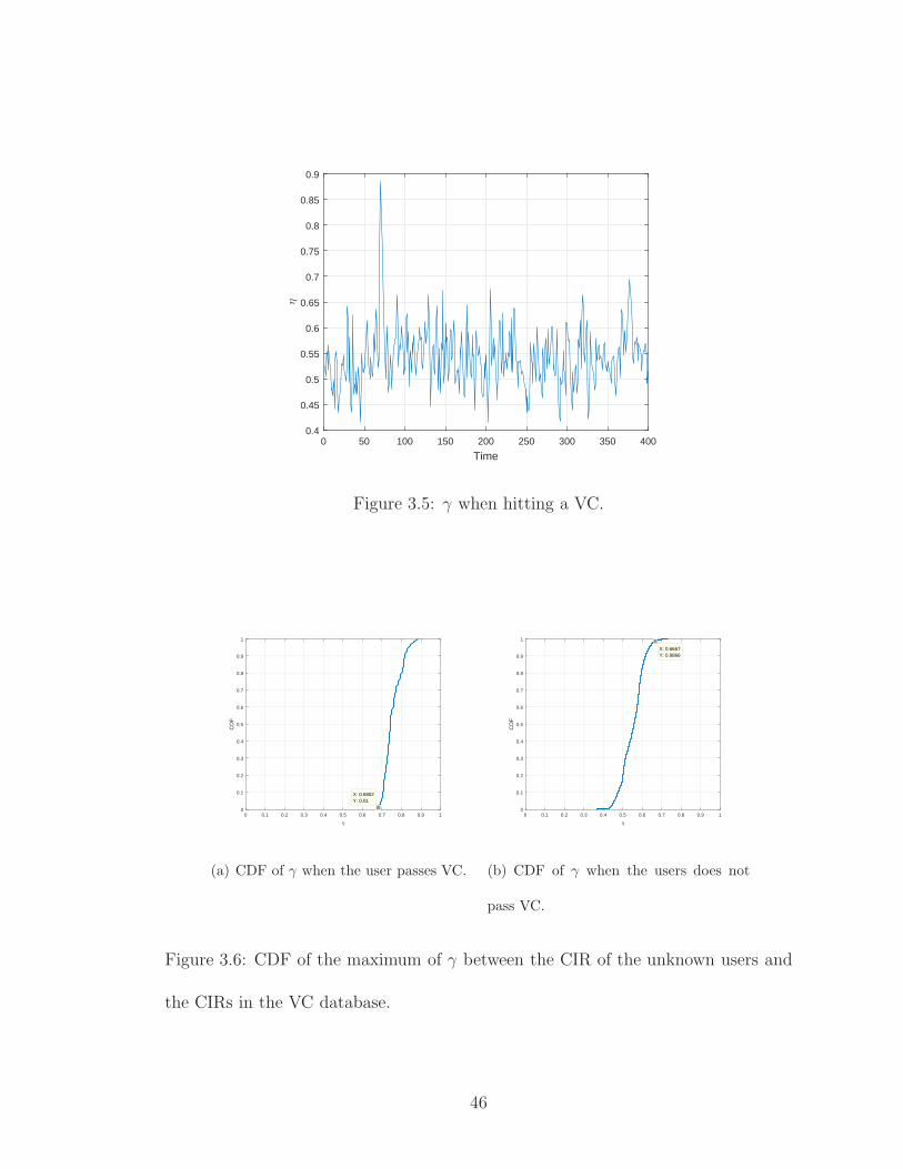
0 50 100 150 200 250 300 350 400

Time

0.4

0.45

0.5

0.55

0.6

0.65

0.7

0.75

0.8

0.85

0.9

η

Figure 3.5: γ when hitting a VC.

0 0.1 0.2 0.3 0.4 0.5 0.6 0.7 0.8 0.9 1

η

0

0.1

0.2

0.3

0.4

0.5

0.6

0.7

0.8

0.9

1

CD

F

X: 0.6802Y: 0.01

(a) CDF of γ when the user passes VC.

0 0.1 0.2 0.3 0.4 0.5 0.6 0.7 0.8 0.9 1

η

0

0.1

0.2

0.3

0.4

0.5

0.6

0.7

0.8

0.9

1

CD

F

X: 0.6667Y: 0.9866

(b) CDF of γ when the users does not

pass VC.

Figure 3.6: CDF of the maximum of γ between the CIR of the unknown users and

the CIRs in the VC database.

46

0 0.1 0.2 0.3 0.4 0.5 0.6 0.7 0.8 0.9 1

False Alarm Prob.

0

0.1

0.2

0.3

0.4

0.5

0.6

0.7

0.8

0.9

1

Det

ectio

n P

rob.

Figure 3.7: ROC of VC detecction.

3.6 Discussion

We discuss some issues concerning to the implementation of VC in this Section.

• The γ Waterlevel: The TRIPS declares the unknown user to be at the VC

when the γ of the received CIR and the CIR from the VC is larger than a

threshold. This simple detection algorithm produces false alarm when the

target passes through locations with higher γ is calculated using the CIRs

around the VC, which we call the γ waterlevel. The γ waterlevel is different

for each of the VC and the waterlevel is affected by the environment, such as

the LOS, NLOS setting, the room layouts, etc. A uniform threshold for all the

VCs raises the false alarm and gives the wrong location estimate which causes

47

trouble for following tracking algorithms. Therefore, an optimal threshold of

for each VC shall be found considering the statistical behavior of γ around the

virtual checkpoint.

• Hardware Consistency: The RF component used for VC CIR collection and

the RF component used by the user are not the same one in general cases.

Therefore, the hardware inconsistency between each RF interface shall be con-

sidered when the system is implemented. The inconsistency causes a lowered

γ even if the target is in the VC, which results in a higher false alarm rate.

Experiments show that the hardware consistency can be accountable for a 0.3

drop in γ in some cases.

• Database Size: The database size is related to size of the VC. In order for the

user to transmit at least one CIR probing signal when passing through the VC,

the CIR has to be dense enough. Also, the user’s speed and the transmitting

frequency also constraints the thickness of the VC, which also affects the size

of the final VC database. When we factor in multiple VCs in the system,

the computation load may be intense and parallelization is needed. For the

current VC, we have 6 cm in the depth, 6 cm in height, and about 75 cm

in width, with 1 cm resolution at all dimensions, and each CIR realization is

2816 bytes. Therefore, the database size for one VC is about 7.6 MB.

• Side Information: The location detection via VC only detects user at the VC,

where the exact location of the user between VCs is not clear. In order to

get the estimate of the user between checkpoints, side information from other

48

sensors can provide an estimation between VCs. Also, the estimated location

can also narrow the set of VCs that the VCTR system has to calculate the γ

using the received CIR.

3.7 Summary

In this chapter, we propose a novel indoor tracking system that track the target

via virtual checkpoint. The essence of the construction of virtual checkpoint stems

at the spatial temporal focusing effect of the TR system as shown in Chapter 2,

where location identification is possible using the location-specific CIR information.

We built a prototype machine for collecting CIR information which operates auto-

matically. We then verify the virtual checkpoint concept via a simple path and a

virtual checkpoint. The experiment data shows that the proposed virtual checkpoint

captures the activity of the user and gives estimation of the target’s location.

49

Chapter 4

Time Reversal Medium Access Control

In previous chapters, we have developed and verified the performance of the

TR indoor positioning system based on the unique spatial temporal focusing effect.

The location-specific CIR, on the other hand, also benefits the TR system with

the spatial temporal focusing effect [55] that focuses the transmitted energy to the

intended user. By selecting the waveforming signature as the time-reversed and

conjugated version of the intended receiver’s CIR, the transmitted waveform adds

up constructively at the exact location of the intended receiver, while the waveform

adds up randomly at all other locations. The receiver receives maximum signal

energy with small energy leakage to surrounding users. The energy focusing due

to location-specific CIR information separates TR users operating on the same fre-

quency band and allows simultaneous access, leading to the design of time reversal

division multiple access (TRDMA) system that provides service to a large amount

of users [20].

The other 5G candidate, the massive MIMO system, achieves the energy fo-

cusing by using a large number of antennas [29]. The massive MIMO system con-

centrates the transmitted energy at the intended user by adjusting the weight vector

of the antennas, which is known as beamforming. With the increase of the number

50

of antennas, the massive MIMO system directs the energy to more intended users

with small energy leakage to the unintended users, and therefore the system is able

to supports lots of users.

However, with the ever-increasing number of users in the foreseeable IoT fu-

ture, the 5G systems cannot indefinitely support all users simultaneously due to the

fixed usable bandwidth and/or the fixed number of antennas. Interference among

the users will increase and the energy focusing effect can no longer support the mas-

sive users with satisfactory quality of service (QoS). As a result, a system scheduler

that dictates when and whom to access the system simultaneously and maximizes

the system performance is desirable. The scheduler also requires a reasonable com-

plexity in order to operate in real time with strict scheduling deadlines.

Many existing systems already have schedulers deployed, however, none can

be implemented directly on the TR and the massive MIMO system. There are

two main reasons. The first is the fundamental differences in the physical layer

design. In existing and widely deployed OFDMA systems, such as the LTE system,

the scheduler allocates the resource blocks (RBs) that are mutually orthogonal in

time and frequency to users. The RBs are allocated based on system requirements

such as the QoS awareness of the users [28, 46, 52] or the weighted sum rate of the

overall system [23]. However, in the case of TR system, the transmission resource

is not mutually orthogonal and all the users are using the same transmission band.

Therefore a new scheduler design is needed to select a subset of users for transmission

while managing the in-band interference. On the other hand, although OFDMA

can be an element for massive MIMO system, the interference between users still

51

exists for the users on the same frequency band and interference management is still

desirable.

The second reason is that with the massive number of users in the system,

it is possible that the system cannot accommodate the users simultaneously via

power control. In a typical power control scheme, the system adjusts the transmit

power to different users in order to control the interference introduced to unintended

users [24, 39, 59]. However, when a massive number of users are present in the

system, all the proposed power allocation based algorithm might not be feasible due

to minimum transmitted power requirements of the users. The system therefore

needs to efficiently select a subset of users for transmission that not only maximizes

the system objective but also meets the individual QoS requirements.

In a scheduler design, it is usually assumed perfect channel information, whereas

the channel information is imperfect in reality. Several factors contribute to the im-

perfect channel information including the aging of the channel, the received noise

during channel estimation, the pilot contamination between users, and so on. The

imperfect channel information not only degrades the performance of the physical

layer, but also deteriorates the scheduler performance. Robustness against imper-

fect channel information in scheduler design is therefore highly desirable to sustain

the system performance when the channel information is inaccurate.

In order to address the above issues, we propose a novel medium access control

(MAC) layer scheduler design by taking into consideration of the unique focusing

effect for both the TR and massive MIMO system. In the first part of the chapter,

we focus on the scheduler algorithm that selects a subset of users and maximizes the

52

system weighted sum rate. The optimization problem is transformed and formulated

as a mixed integer quadratically constrained quadratic program (MIQCQP) [53]

where the optimization problem is solved using an optimization solver. In the second

part, we focus on the impact of imperfect channel information on the scheduler

performance. We analyze a channel estimation scheme for TR system proposed

in [36] and identify similar channel estimation error distribution as in the massive

MIMO case. We evaluate the robustness of the proposed scheduler against imperfect

channel information provided by the channel estimation scheme.

The main summary of this chapter is as follows:

1. We propose an efficient scheduler algorithm for 5G system that maximizes the

weighted sum rate by selecting a subset of users for transmission. The system

objective and QoS constraints are transformed into a MIQCQP with empirical

linear time complexity.

2. We analyze the channel estimation error distribution of the TR system. Anal-

ysis shows that the TR channel estimation scheme reduces the channel esti-

mation error power and reveals a similar estimation error distribution as in

the massive MIMO case.

3. We evaluate the proposed scheduler under imperfect channel information. Ex-

periment results show that the proposed scheduler is robust against imperfect

channel information with small performance degradation.

The chapter is organized as follows. System description for both the TR and

massive MIMO system is given in Sec.4.1. The energy focusing effect of both TR

53

and massive MIMO systems is illustrated via simulation in Sec.4.2. The scheduler

objective and user requirements are described in Sec.4.3 and the MIQCQP formu-

lation is developed. In Sec.4.4, we investigate the impact of the imperfect channel

information on the performance of the scheduler. Simulation results are presented in

Sec.4.5 where the performance of the scheduler is evaluated under various settings.

Finally, a conclusion is given in Sec.4.6.

4.1 System Overview

We give brief overviews of the TRDMA downlink system and the massive

MIMO downlink system and introduce the spatial focusing effect of both systems.

4.1.1 Time Reversal Division Multiple Access System

A schematic view of a TRDMA downlink system is depicted in Fig.4.1, where

N users/terminal devices (TD) are served. The access point (AP) first upsamples

the symbol stream for user i by the backoff factor Di. The upsampled symbols are

encoded using the corresponding waveforms gi which are assigned to the users. The

AP transmits the summed signal with a single antenna and the transmitted signal

passes through individual users’ channels hi. The users adjust the power using one

tap gain, downsample the received signal and then perform detection to estimate

and recover the transmitted symbols.

Using the time reversed and conjugated CIR hi between the AP and user i as

the waveform gi, user i obtains the maximum signal power. However, the interuser

54

Figure 4.1: System diagram of a TRDMA system.

interference (IUI) and intersymbol interference (ISI) reduce the SINR of users and

therefore the TR waveform gi can be specifically and jointly designed for the system

to meet system requirements. Several waveforming algorithms have been proposed

in [58] and [57] to alleviate IUI and ISI and to increase the SINR.

4.1.2 Massive MIMO system

Suppose that there are M antennas in the base station serving K one-antenna

terminal devices. The channel hMi from the base station to the user i is an M by 1

vector where the jth element is the channel from the jth antenna to the ith user. We

assume a narrowband massive MIMO system which observes one tap channel due to

the limited subcarrier granularity. Proper beamforming vectors gMi can be designed

to steer the energy to the intended user i, such as the maximum-ratio transmission

and zero forcing beamforming in [42].

The TR system utilizes the time-reversed and conjugated CIR as precod-

ing waveform to transmit the energy to the specific users. Because the CIR are

55

location-specific [55], the energy only concentrates at the intended users with small

energy leakage to the surroundings, which is called the spatial focusing effect. The

large bandwidth enables the TR system to resolve more taps from location-specific

channels and focuses the energy more sharply to the intended user. On the other

hand, the massive MIMO system focuses the energy to the intended users using

the maximum-ratio-combining beamforming weights. By installing more and more

antennas, the massive MIMO system concentrates the energy more sharply at the

intended users as the TR system does with a larger bandwidth. The spatial focus-

ing effect resulting from either larger bandwidth or more antennas enables the 5G

system to pinpoint the energy to the exact users, to reduce the interference leakage,

and therefore to accommodate more users than that in existing systems. In order

to illustrate the spatial focusing phenomenon, we conduct a simulation in both TR

and massive MIMO systems to reveal how the focusing effect becomes prominent

with the increase in either bandwidth or the number of antennas.

4.2 Spatial Focusing Effect

With proper waveform design gi and beamform weight design gMi , both the

systems focus energy only at the intended users. The ability of the energy trans-

mission targeting at specific users is affected by the degree of freedom (DoF) of the

design, which is the number of variables in gi or gMi . The TR system increases the

DoF by using a large bandwidth which results in a massive number of observed CIR

taps, while the massive MIMO system increases the DoF by installing a massive

56

number of antennas. The larger the bandwidth and the number of antennas, the

larger DoF, and therefore the better spatial energy focusing at the locations of the

intended users.

To illustrate the spatial focusing effect of both systems with different DoF,

we conduct a simulation based on ray-tracing techniques in a discrete scattering

environment. 400 scatterers are distributed randomly in a 200λ× 200λ area, where

λ is the wavelength corresponding to the carrier frequency of the system. The

wireless channel is simulated by calculating the sum of the multipaths using the

ray-tracing method given the locations of the scatterers. Without loss of generality,

we use a single-bounce ray-tracing method to calculate the channels for both the

TR system and the massive MIMO system on the 5GHz ISM band. We select the

reflection coefficients of the scatterers to be i.i.d. complex random variables with

uniform distribution in amplitude [0, 1] and phase [0, 2π]. For the massive MIMO

system, the linear array is configured with the line facing the scattering area and the

interval between two adjacent antennas is λ/2. The distance from the transmitter

and the intended location is chosen to be 500λ for both systems.

To show the effect of system DoF on the spatial focusing effect, we adjust

the transmitting bandwidth of the TR system and the number of antennas in the

massive MIMO system. The transmitter of the TR system transmits with band-

widths ranging from 100 MHz to 1GHz with one antenna, where a wider bandwidth

observes more CIR taps and increases the system DoF. The number of antennas in

the massive MIMO system is selected from 20 to 100 with bandwidth fixed at 1MHz

in the simulation. We select the matched filter waveform and beamforming weights

57

MM-20Antennas

x-axis ( /20)

20 60 100

y-a

xis

(

/20) 20

40

60

80

100 -10

-8

-6

-4

-2

0MM-40Antennas

x-axis ( /20)

20 60 100

y-a

xis

(

/20) 20

40

60

80

100 -10

-8

-6

-4

-2

0MM-100Antennas

x-axis ( /20)20 60 100

y-a

xis

(

/20) 20

40

60

80

100 -10

-8

-6

-4

-2

0

(dB)(dB)(dB)

(a) Normalized field strength in a 5λ×5λ area centered around the receiver of a massive MIMO

system.

TR-100MHz

x-axis ( /20)20 60 100

y-a

xis

(

/20) 20

40

60

80

100 -10

-8

-6

-4

-2

0TR-200MHz

x-axis ( /20)20 60 100

y-a

xis

(

/20) 20

40

60

80

100 -10

-8

-6

-4

-2

0TR-1000MHz

x-axis ( /20)20 60 100

y-a

xis

(

/20) 20

40

60

80

100 -10

-8

-6

-4

-2

0

(dB)(dB)(dB)

(b) Normalized field strength in a 5λ× 5λ area centered around the receiver of a TR system.

Figure 4.2: Demonstration of the spatial focusing effect for both TR and massive

MIMO systems with different DoF.

58

in the TR system and the massive MIMO system, respectively.

We consider the received energy strength in a 5λ×5λ area around the location

of the intended user. Fig. 4.2 shows the simulation results for both systems with

a single channel and scatterer realization, and we normalize the maximum received

energy to 0dB. We can see that the energy focusing effect becomes more obvious

at the intended location with the increase in the bandwidth and the number of

antenna, which is the result of larger DoF to concentrate the energy at only the

intended users.

However, a closer look at the energy field in Fig. 4.2 reveals that even with

large transmitting bandwidth and massive number of antennas, energy leakage still

occurs at the surrounding of the intended users. The energy leakage causes the

IUI and the interference level increases when the number of users grows. Scheduler

design is therefore desirable to perform interference management by selecting a

subset of users for transmission. In essence, the user selection is to choose a subset

of users such that the energy leakage has small interference to any of the other

selected users in order to reduce the IUI and to increase the total transmission rate.

4.3 Downlink User Selection Algorithm

In this section, we detail the algorithm for maximizing the weighted sum rate

in the downlink system. To be specific, the scheduler receives the normalized inter-

ference matrix and the allocated transmission power for each of the users from the

physical layer and the minimum required transmission rate for the user from the ap-

59

plication layer. The scheduler maintains weights for the users to adjust the fairness

and to avoid starving due to poor channel condition and shadowing. Based on the

information, the scheduler selects a subset of users to transmit simultaneously and

maximizes the weighted sum rate while satisfying the minimum SINR requirement

for the selected users.

4.3.1 TRDMA System Overview

First let us characterize the received signal of the users in a TRDMA downlink

system. Suppose that there are N users in the system and all users use the same

backoff factor D. Xi[m] is the transmitted symbols to user i, which is assumed to

be i.i.d. with unit power. Based on the system structure in Fig. 4.1, the transmit

signal of the AP can be expressed as

s[m] =∑

i

∑

l

√pigi[m− l]X

[D]i [l], (4.1)

where X[D]i represents the upsampled version of the symbols to user i by D, pi is

the allocated transmit power and gi denotes the designed transmitting waveform

with unit power for user i. User i receives the signal and downsamples the signal

for detection, and the downsampled signal can be expressed as

60

Yi[m] =

N∑

j=1

∑

l

√

GjpjXj [l](hi ∗ gj)[mD − lD] + ni[m]

=√

GipiXi[m](hi ∗ gi)[L− 1] +√

Gipi

2L−2D∑

l=0,l 6=L−1D

Xi[m− l](hi ∗ gi)[Dl]

+∑

j 6=i

√

Gipj

2L−2D∑

l=0

Xj[m− l](hi ∗ gj)[Dl] + ni[m],

(4.2)

where hi is the channel from AP to user i with unit power. L is the length of hi,

which depends on the delay spread of the environment and the utilized bandwidth

of the system. With our measurement using TR system prototype with 125 MHz

bandwidth, we observe about 10 significant CIR taps and the total channel length

L is about 30. For notation brevity, we assume that L− 1 is an integer multiple of

the backoff factor D. Gi is the path gain from the AP to user i. Note that the hi

is unit power and the channel power is absorbed into Gi. ni is the receiving noise

of user i and is assumed to be an i.i.d. complex Gaussian r.v. with power σ2i . In

(4.2), the first term represents the intended signal for user i; the second term is the

ISI; the third term is the IUI and the last term is the receiving noise.

4.3.2 Normalized Interference Matrix Calculation

Let us characterize the interference between the users based on the unit power

channel hi and the waveforms gi. The (i, j)th entry Zi,j of the normalized inter-

ference matrix Z refers to the interference from user j to user i. Therefore, Zi,j is

determined by the channel hi from the AP to the user i and the waveform gj used

transmit to user j. Zi,j is calculated using unit power hi and unit power gj , and

61

therefore the name normalized interference matrix. We separate pj in the calcu-

lation of Zi,j because the power allocation and the waveforms are not necessarily

designed together and the separation expands the occasions where the scheme is

applicable. Based on (4.2), the normalized interference between users can therefore

be represented as

Zi,j =

2L−2D∑

l=0

|(hi ∗ gj)[Dl]|2 , (4.3)

Zi,i =

2L−2D∑

l=0

l 6=L−1D

|(hi ∗ gi)[Dl]|2 , (4.4)

where (4.3) and (4.4) are the IUI and ISI for user i, respectively. On the other hand,

the IUI for the massive MIMO system can be calculated as

Zi,j =∣

∣(hMi )TgM

j

∣

∣

2, (4.5)

there is no ISI in the massive MIMO system due to the assumption of limited

subcarrier granularity and a single tap channel is observed.

4.3.3 Scheduler Objective

Let us first formulate the scheduler objective and the constraints. Suppose that

the physical layer provides the scheduler with the normalized interference matrix Z

between users, the allocated power p and the path gain Gi between the AP and user

i. The scheduler gathers the transmission rate requirements Ri from the application

layer for proper operation if user i is selected to transmit. For a specific transmission

62

rate requirements Ri, we can obtain the corresponding minimum SINR requirement

γi by the one to one mapping between rate and SINR. The scheduler maintains a

set of weights wi to indicate the relative importance of each user. Based on the

collected information and requirement, the scheduler objective that maximizes the

system weighted sum rate is formulated as

maximizex

∑

i

wixi log2

(

GipiGi

∑

j pjZi.jxj + σ2i

+ 1

)

subject to xi ∈ {0, 1},∑

i

pixi ≤ Pmax,

Gipixi

Gi

∑

j pjZi,jxj + σ2i

≥ γixi, ∀i.

(4.6)

The first constraint requires the decision variables xi to be binary, and xi = 1

represents user i is selected to transmit. The second constraint requires that the sum

of the transmitting power of the selected users to be no more than the maximum

AP transmitting power. The third set of constraints correspond to the minimum

SINR requirements γi that the selected users must meet, and therefore the selected

users meet the minimum transmission rate requirement Ri.

4.3.4 Mixed Integer Optimization

Let us describe the optimization transformation here. By enumerating all

possible x vectors, we can find the optimal decision vector xopt that maximized the

objective and meet all the SINR constraints. However, the complexity for complete

enumeration grows exponentially with the number of users N and therefore enumer-

ation is not feasible when the number of users grows big. In this section, we propose

63

a simple yet effective problem formulation that transforms the objective and the

constraints into a MIQCQP problem.

One property for binary decision variables that is used in the optimization

formulation is as follows,

x2i = xi, ∀i. (4.7)

This relationship helps convert some of the quadratic terms into linear terms in the

system objective and the constraints.

We consider that the scheduler operates at the high SNR region where we omit

the noise term σ2i at the receiver and the plus 1 term in the logarithm function. Also,

the path gain Gi cancels each other and the optimization objective becomes

maximizex

∑

i

wixi log2

(

pi∑

j pjZi,jxj

)

subject to xi ∈ {0, 1},∑

i

pixi ≤ Pmax

pixi∑

j pjZi,jxj + σ2i /Gi

≥ γixi, ∀i

(4.8)

We decompose the objective function into two terms using characteristics of

the logarithm function as the following

maximizex

∑

i

wixi log2

(

pi∑

j pjZi,jxj

)

≡ maximizex

∑

i

wixi ln pi −∑

i

xiwi ln

(

∑

j

pjZi,jxj

)

.

(4.9)

Next, we linearize the second logarithm term using the Taylor expansion of

logarithm at x0 = 1 and use the constant term and the first order term. Note that the

64

Taylor expansion for logarithm function to the linear term is a global overestimator

of the logarithm function.

Let p, w be the power and weight vector of length N of the users respectively.

The second term in (4.9) can be simplified as

∑

i

wixi ln

(

∑

j

pjZi,jxj

)

≤∑

i

wixi

(

∑

j

pjZi,jxj

)

−wTx

= xT (diag(w)Zdiag(p))x−wTx,

(4.10)

where diag(·) operation generates a diagonal matrix using the elements in the vector.

The inequality comes from the upper bound of Taylor expansion of the natural

logarithm to the linear term. Define A = diag(w)Zdiag(p) and ◦ as the Hadamard

product of two vectors. The objective function can be represented as

∑

i

wixi ln

(

pi∑

j pjZi,jxj

)

≥ (ln(p) ◦w)Tx− xTAx+wTx (4.11a)

= (ln(p) ◦w +w)Tx− 1

2xT (A+AT )x, (4.11b)

where (4.11a) follows the property of Taylor expansion. The original objective func-

tion is transformed into (4.11b). However, it is not guaranteed that the optimal

vector xopt for (4.9) and (4.11b) are the same.

Define IN as an identity matrix of size N and 1 be an all 1 vector of corre-

sponding size, we addc

2xT INx and subtract

c

21Tx which have the same value by

the property in (4.7), where c is a constant larger than the smallest eigenvalue of

A + AT . Since the same value is added and subtracted in the objective, it does

65

not change the objective value nor the feasible set. The reason for this redundancy

will be discussed in Sec.4.3.5. Define Q = A + AT + cIN , we arrive at the final

formulation as

maximizex

(ln(p) ◦w +w)Tx− 1

2xT (A+AT )x

≡ minimizex

1

2xT (A+AT + cIN)x− (ln(p) ◦w +w +

c

21)Tx

≡ minimizex

1

2xTQx− (ln(p) ◦w +w +

c

21)Tx.

(4.12)

The second constraint can be written as

pTx ≤ Pmax (4.13)

For the third constraint, we have the minimum SINR constraint for user i as,

pixi∑

j pjZi,jxj + σ2i /Gi

≥ γixi (4.14a)

≡ xi

∑

j

pjZi,jxj + (σ2i

Gi

− piγi)xi ≤ 0, (4.14b)

Let 0n,m be a n by m all zero matrix. Define Bi as an all zero matrix with ith

row to be the Hadamard product of zi, the ith row of Z, and the transpose of the

power allocation vector p as follows

Bi =

0i−1,N

zi ◦ pT

0N−i,N

. (4.15)

66

Define qi as an all zero vector of length N , except for the ith component being

σ2/Gi − pi/γi,

qi =

0i−1,1

σ2

Gi

− piγi

0N−i,1

. (4.16)

Then the constraint can be represented as

xTBix+ qTi x ≤ 0, ∀i

≡ 1

2xT (Bi +BT

i + ciIN)x+ (qTi − ci

21)x ≤ 0, ∀i

≡ 1

2xTQix+ (qT

i − ci21)x ≤ 0, ∀i

, (4.17)

where Qi = Bi + BTi + ciIN . ci is a constant that is larger than the minimum

eigenvalue of Bi +BTi .

Based on the above transformation, the whole optimization problem is formu-

lated as

minimizex

1

2xTQx− (ln(p) ◦w +w +

c

21)Tx

subject to xi ∈ {0, 1}, pTx ≤ Pmax

1

2xTQix+ (qT

i − ci21)x ≤ 0, ∀i,

(4.18)

which is an MIQCQP problem if and only if Q and Qis are positive semidefinite.

4.3.5 Positive Semidefiniteness of Q and Qi

To ensure the transformed optimization problem to be an MIQCQP problem,

we need to ensure Q and Qi are all positive semidefinite. We first introduce the

Weyl theorem [22] which states as follows.

67

Theorem 1 Let U, V be Hermitian matrices of size N and let the eigenvalues

λi(U), λi(V), and λi(U+V) be arranged in non-decreasing order. For k = 1, 2, · · · , N ,

we have

λk(U) + λ1(V) ≤ λk(U+V) ≤ λk(U) + λn(V) (4.19)

Take U as A +AT and V as cIN . It is clear that if c ≥ λ1(A +AT ) then Q

will be positive semidefinite. The same also applies to Qi and the constants ci for

the constraints.

The calculation for the eigenvalue for both the objective function and each

of the constraints might seem time consuming. Nevertheless, we can simply use

a predefined constant rather than calculating the eigenvalue for each optimization

problem. In our simulation, simply choosing c = ci = 1 is sufficient to ensure a valid

MIQCQP formulation.

4.3.6 Extension to Multi-Cell Scenarios

We propose an scheduler based on the MIQCQP formulation in a downlink,

single-cell setting in previous sections. The same formulation methodology can be

applied to downlink cooperative multipoint (CoMP) scenarios with changes in the

definition of variables and in the derivation of the normalized interference matrix Z.

Let us consider a downlink scheduler in a multi-cell network with C full frequency-

reusing and synchronized cells. Suppose that Nk users are in cell k, k = 1, · · · , C,

and there is inter-cell interference (ICI) due to full frequency reuse among cells.

68

To distinguish the users in different cells, we use superscript to indicate the

index of the cell, and use subscript to indicate the user in a specific cell. Define hk,li

as the normalized CIR from cell l to user i in cell k and define glj as the transmitting

waveform assigned to user j in cell l. Define Gk,li as the path gain from cell l to the

user i in cell k. Suppose all users in all cells use the same backoff factor D, then the

downsampled received signal for user i in cell k can be expressed as

Y ki [s] =

C∑

c=1

Nc∑

u=1

∑

t

√

Gk,ci pcuX

cu[t](h

k,ci ∗ gcu)[sD − tD] + nk

i [s]

=

√

Gk,ki pkiX

ki [s](h

k,ki ∗ gki )[L− 1] +

√

Gk,ki pki

2L−2D∑

t=0,t6=L−1D

Xki [s− t](hk,k

i ∗ gki )[Dt]

+∑

j 6=i

√

Gk,ki pkj

2L−2D∑

t=0

Xkj [s− t](hk,k

i ∗ gkj )[Dt]

+

C∑

c=1,c 6=k

∑

j

√

Gk,ci pcj

2L−2D∑

t=0

Xcj [s− t](hk,c

i ∗ gcj)[Dt] + nki [s],

(4.20)

where the first term is the received signal, the second term the ISI, the third term

the IUI, the fourth term is the ICI, and the last term is the receiving noise.

Let Zk,k denote the Nk by Nk normalized interference matrix within cell k as

defined in Sec.4.3.2. Let Zk,l be the Nk by Nl ICI matrix. Zk,li,j , the (i, j)th term of

Zk,l, represents the ICI to the user i in cell k due to the transmitted signal to user

j in cell l. Zk,li,j is defined as

Zk,li,j =

2L−2D∑

t=0

Gk,li

Gk,ki

∣

∣

∣(hk,l

i ∗ glj)[Dt]

∣

∣

∣

2

, (4.21)

69

where Gk,ki in the denominator is to cancel the same term later in the formulation.

We can define the normalized interference matrix Z in the multi-cell scenario as

Z =

Z1,1 Z1,2 · · · Z1,C

Z2,1 Z2,2 · · · Z2,C

......

. . ....

ZC,1 ZC,2 · · · ZC,C

. (4.22)

Let N =∑C

k=1Nk be the total number of users in all cells, and we define

the new decision variable vector of length N as x = [xT1 xT

2 · · · xTC ]

T , and the

new power vector of length N as p = [pT1 pT

2 · · · pTC ]

T . The total interference

Iki including ISI, IUI and ICI to user i in cell k is

(

Gk,ki Zdiag(p)x

)

[∑k−1

c=1 Nc + i],

where the term in (·) is a vector of length N , and the operator [·] takes out the

corresponding element in the vector.

The weighted sum rate maximization in (4.6) can be reformulated using the

newly defined variables and interference matrix as

maximizex

∑

k

∑

i

wki x

ki log2

Gk,ki pki

(

Gk,ki Zdiag(p)x

)

[∑k−1

c=1 Nc + i] + (σki )

2+ 1

subject to xki ∈ {0, 1}, ∀i, k,

∑

i

pki xki ≤ P k

max, ∀k,

Gk,ki pki x

ki

(

Gk,ki Zdiag(p)x

)

[∑k−1

c=1 Nc + i] + (σki )

2≥ γk

i xki , ∀i, k,

(4.23)

where user i in cell k has its own corresponding weight wki , SINR requirements γk

i ,

and receiving noise (σki )

2. The same procedure follows to transform the optimization

70

problem into the MIQCQP formulation. In the CoMP setting, it is assumed that

the scheduler has the full knowledge of the path gain, channels and waveforms of

the system. If the full knowledge of the system is too expensive to obtain, some of

the components can be approximated and the MIQCQP formulation still applies.

4.4 Impact of Imperfect Channel Information

In the previous Section, we assume that the CIR information provided by

the physical layer to be perfect. However, the CIR information provided by the

physical layer is subject to receiving noise. Mismatch between the true and the

estimated channel causes worse energy focusing in the 5G system, which results in a

lower SINR in communication. Moreover, the mismatch also degrades the scheduler

performance by noisy physical layer parameter inputs.

To investigate the impact of imperfect channel information, we start from

analyzing the channel estimation error of the physical layer. There are existing

literature on the distribution of the channel estimation error for the massive MIMO

system [40], but there is no existing analysis or models on the channel estimation

error on the TR system. Therefore, we first analyze a Golay sequence based channel

estimation scheme for TR system proposed in [36] and analyze its impact on the

accuracy of scheduler parameter inputs.

71

50 100 150 200 250 300 350 400 450 500-50

0

50

100

150

200

250

300

(a) Ga.

50 100 150 200 250 300 350 400 450 500-50

0

50

100

150

200

250

300

(b) Gb.

50 100 150 200 250 300 350 400 450 5000

100

200

300

400

500

600

(c) Corr(Ga,Ga) +

Corr(Gb,Gb).

Figure 4.3: An example of Golay sequence.

4.4.1 Golay Sequence Based Channel Estimation

The Golay complementary sequence is first proposed in [17], which suggested

a set of complementary sequence pairs Ga and Gb of the same length LG. The

correlation of Ga with itself, i.e. Corr(Ga,Ga) has a prominent peak but noisy

sidelobes. However, Corr(Ga,Ga)+Corr(Gb,Gb) produces a single maximum peak

with no sidelobes. This prominent peak is useful in channel estimation because a

clean copy of channel estimation can be obtained at the peak without the interference

from the sidelobes.

Generation of Ga and Gb is based on two different sequences Dn and Wn of

length n, and the length of the generated Golay sequence is LG = 2n. Fig. 4.3

shows an example of Ga and Gb pair using randomly generated Dn and Wn with

LG = 256, and Corr(Ga,Ga) + Corr(Gb,Gb) shows a clear peak with no sidelobes.

Please note that the amplitude of the peak is 2LG and the length of the zero at the

two sides of the peak is LG − 1.

72

Figure 4.4: Diagram for Golay based channel estimation.

4.4.2 Channel Estimation via Golay Sequence

A channel estimation scheme using a 8LG by 1 probing sequence φ is proposed

in [36], which is composed of the corresponding pair of Golay sequences Ga,Gb as

φ = [GTa GT

b −GTa GT

b GTa −GT

b GTa GT

b ]T . (4.24)

Fig. 4.4 shows the block diagram of the channel estimation. The transmitter

transmits the channel estimation sequence φ and the receiver receives the L+8LG−1

by 1 signal s = φ ∗ h+ n, where L is the length of h. We assume n is AWGN with

zero mean and variance σ2.

The received signal s is divided into two branches. One branch goes through

a delay of 2LG and is summed with the other branch as Rd.

Rd =

IL

02LG,L

+

02LG,L

IL

s. (4.25)

We calculate the correlation of Rd with Ga and Gb using the Golay correlator

block, which produces two branches Ra and Rb, respectively. Define Ca and Cb as

the L + 3LG − 1 by L + 2LG convolution matrix constructed by the time reversed

version of Ga and Gb, and the outputs of the Golay correlator can be expressed as

73

Ra = CaRd and Rb = CbRd. Rb is delayed by 3LG to summed with Ra in order to

produce the final channel estimation result. Therefore, the whole estimation block

can be expressed as

y =

IL+3LG−1

02LG,L+3LG−1

CaRd +

02LG,L+3LG−1

IL+2LG−1

CbRd

= T (φ ∗ h+ n) =

T1

Φ

T2

(φ ∗ h+ n).

(4.26)

The matrix T is the total transfer function from the estimation block input s

to the block output, and it is separated into three parts T1,Φ, and T2 by the rows.

T1 and T2 represent the noisy part of the channel estimation scheme which is the

sidelobes of the correlation of Ga and Gb, and these two parts are of no interest

in channel estimation. Φ is the 7LG-th to the 8LG-th rows that correspond to the

clean peak of the correlation of the Golay sequences without sidelobes, as shown in

Fig. 4.3(c). Φ is a matrix that is determined by the Golay sequence pair, and each

row of Φ has exact 4LG none zeros entries with amplitude 1.

The channel estimation h of length LG + 1 can therefore be represented as

h = Φ(φ ∗ h+ n) = 4LGh′ + Φn = 4LGh

′ + ne, (4.27)

where h′ is of length LG+1 which is formed by zero-padding h to match the matrix

dimension, and ne is the channel estimation error due to the received noise n at the

receiver.

74

4.4.3 Channel Estimation Error Analysis

We investigate the mean and variance of ne to show the effect of n and LG on

the quality of channel estimation. By the assumption that n is AWGN with zero

mean and variance σ2, the mean of estimation error ne is also zero. The covariance

of the channel estimation error ne is ΦCov(n)ΦH . It is assumed that n is i.i.d.

AWGN with variance σ2, and therefore the covariance of ne is σ2ΦΦH .

To give an example of the correlation of ne, we randomly generate a Golay

sequence pair with LG = 256. Fig. 4.5 is the correlation of ne with n to be

i.i.d. Gaussian with unit σ2, namely ΦΦH . The prominent diagonal components

have value 4LG and each element of the diagonal is the noise variance σ2e of ne.

The off-diagonal components have extremely low value, which shows that different

components of ne are almost uncorrelated. Therefore, the channel estimation errors

ne on each tap of the estimated channel h′ are nearly uncorrelated, which is nearly

independent due to the assumption that n is i.i.d. AWGN.

4.4.4 SNR Enhancement of Golay Sequence Based Channel Estima-

tion

The Golay sequence based channel estimation scheme increases the SNR of

the channel estimation. Suppose that the SNR at the receiver is P/σ2 where P

and σ2 are the power of the received signal s and the noise n, respectively. The

channel estimation output has a peak with amplitude 4LG, by which the power of

the channel estimation is 16L2GP . Each row of Φ consists of exactly 4LG none zero

75

50 100 150 200 250

50

100

150

200

250 0

100

200

300

400

500

600

700

800

900

1000

Figure 4.5: An example of ΦΦH .

elements with amplitude 1, therefore σ2e is 4LGσ

2. As a result, the SNR at the

channel estimation output is boosted for 4LG times.

The channel estimate using the proposed Golay channel estimation scheme

is contaminated with noise which has zero mean and variance 4LGσ2. Therefore,

the length of the Golay sequence affects the SNR boost at the estimation output,

and the TR system can adapt the Golay sequence length LG based on the system

requirement on channel estimation. More importantly, ne on each tap of the channel

estimation are nearly independent, which is the result from the structure of the

transfer function Φ of the Golay channel estimation scheme.

The channel estimation error for the massive MIMO system is investigated

in [40]. The channel estimation errors on the links from the base station to a user

are i.i.d. complex Gaussian with zero mean and same variance which is determined

by the shadowing effect of the user. The channel estimation error of the TR system

76

and the massive MIMO system share similarity in that the estimation error of the

channel are i.i.d variables with zero mean and the same variance. This similarity in

channel estimation error therefore extends the discussion and simulation results on

the scheduler performance degradation to massive MIMO counterparts.

4.4.5 Effect on the Scheduler Parameter

The proposed scheduler algorithm generates the transmission profile for the

users based on the estimated channel and the assigned power from the physical

layer. Inaccurate channel estimation deteriorates the efficiency of the scheduling in

the MAC layer, and it is desirable to investigate how the channel estimation error

affects the input parameter of the proposed scheduler.

Based on the previous investigation of the channel estimation error, we model

the estimated channel h as

h = h+ ne, (4.28)

where we assume that ne is i.i.d. complex Gaussian noise with zero mean and vari-

ance σ2e . According to the optimization formulation of the scheduler in (4.6), channel

estimation error ne affects the scheduler performance by affecting the calculation of

the normalized interference matrix Z. Define Z as the normalized interference ma-

trix obtained using the channel estimation h, and we calculate the expectation of

Z to show the impact of channel estimation error on the normalized interference

matrix Z.

77

E

[

Zi,j

]

= E

2L−2D∑

l=0

∣

∣

∣(hi ∗ gj)[Dl]

∣

∣

∣

2

= E

2L−2D∑

l=0

∣

∣

∣((hi + ne) ∗ gj) [Dl]

∣

∣

∣

2

=

Zi,j +σ2

4LG

(

L− 1

D− 1

)

+σ2

4LG

L−1D∑

l=0

∣

∣

∣gj [Dl]

∣

∣

∣

2

,if i = j

Zi,j +σ2

4LG

(

L− 1

D

)

+σ2

4LG

L−1D∑

l=0

∣

∣

∣gj[Dl]

∣

∣

∣

2

,if i 6= j

<

Zi,j +σ2

4LG

(

L− 1

D

)

,if i = j

Zi,j +σ2

4LG

(

L− 1

D+ 1

)

,if i 6= j

(4.29)

where the last inequality results from the normalized waveform gj and serves as an

upper bound for E[

Z]

.

The formula suggests that the error in the normalized interference matrix

∆Z = E

[

Zi,j

]

− Zi,j relates to three factors, the backoff factor D, the channel

length L, and the length of the Golay sequence LG. A larger backoff factor not only

reduces the IUI and ISI but also reduces the impact of the channel estimation error

on the normalized interference matrix. The longer the channel length, the larger the

IUI and ISI, thus the bigger ∆Z. The last factor is the Golay sequence length LG,

which affects the additive noise power at the channel estimation. The dependence

of ne on LG gives the system the flexibility to adapt the length of Golay sequence

to the users’ SNR conditions.

78

4.5 Simulation Results

In this section, we evaluate the performance of the proposed scheduler algo-

rithm from several aspects. First, we compare the time complexity of the proposed

scheduler algorithm with that using enumeration. We also evaluate the scheduler

performance under different physical layer structures. Then we investigate the im-

pact of channel estimation error. We use the following model and system parameters.

We generate h of the TR system based on the channel model proposed in [20], and

waveform g is the time reversed and conjugated version of h. For TR system, users

are distributed randomly within a 20 meter by 20 meter area with the transmit-

ter located at the center to simulate an indoor environment. For massive MIMO

system, users are distributed randomly within a 300 meter by 300 meter area to

simulate an outdoor environment. The transmitter is located at the center of the

area in both cases. The path loss exponent is 3.5. The rate requirements for the

users Ri are generated uniformly from the range of 1 Mbps to 2 Mbps. The weight

vector w is generated uniformly from 0 to 1. The power vector is generated from a

uniform distribution from 0.1 to 0.3 for each user and Pmax is set to 1. The SNR is

0 dB for each of the users, unless mentioned otherwise. The system bandwidth of

the TR system is 125 MHz in the simulation. The simulation is repeated for 2000

channel realizations for each of the settings. Lastly, we select the Gurobi solver to

solve the MIQCQP problem [18].

79

3 4 5 6 7 8 9 10Number of users, N

0

0.01

0.02

0.03

0.04

0.05

0.06

0.07

0.08

Exe

cutio

n tim

e in

sec

onds

Exhaustive SearchProposed

Figure 4.6: Run time comparison for different number of users.

4.5.1 Time Complexity

Time complexity is an important performance indication for scheduler that

performs in real time with strict deadline. Moreover, the importance grows with the

foreseeable sharp increase in the number of users in the system. Fig. 4.6 shows the

comparison of the running time with number of users N ranging from 3 to 10 and

D = 4. The proposed scheduler consumes more time than that of exhaustive search

when the number of users are small due to the model setup, and shows an empirical

O(N) complexity. Result shows O(2N) complexity for exhaustive search and the

execution time outpaces the proposed scheduler. The O(N) complexity makes the

proposed scheduler suitable for application with strict deadline.

4.5.2 Scheduling Performance Comparison

To evaluate the performance of the proposed scheduler, we compare the weighted

sum rate of the proposed scheduler RS with the weighted sum rate obtained by ex-

80

haustive search Ropt by calculating the average of the ratio ρ = RS/Ropt. We chose

the backoff factor D = [4, 8, 12, 24, 30] and number of users N = [3, 5, 7, 9]. Fig.

4.7(a) shows the ρ with different N and D. For a small D, the deviation from opti-

mality with large N comes from the errors at the linearization of the logarithm term

around 1, because the actual sum is far from 1. However, when D increases, the

entries of Z becomes smaller and the error due to expansion at 1 gets smaller. For

larger N , which is the targeted use case for the next generation system, ρ increases

rapidly to above 0.9 in all cases where D is larger than 8.

To evaluate the performance of the proposed scheduler under different SNR

conditions, we perform simulations where all users have the same SNR selected from

[−5, 0, 5, 10] dB. We simulate with different backoff factors D = [4, 8, 12, 24, 30] and

N = 9, and the result is presented in Fig. 4.7(b). In the low SNR region, the

approximation in (4.8) is not as accurate and there is a gap between the performance

of the proposed scheduler and that of exhaustive search. However, ρ increases over

0.9 when D is larger than 8 in most SNR cases.

The proposed scheduler separates the physical layer implementation, and the

separation makes the scheduler suitable for different waveform design and power al-

location algorithms. Fig. 4.8(a) shows ρ with a downlink system using the waveform

design and power allocation proposed in [57]. The original uplink max-min SINR

algorithm in [57] is modified using the uplink-downlink duality for downlink pur-

pose. The figure shows a similar ρ as in Fig. 4.7(a), which shows that the proposed

scheduler algorithm is versatile for different physical layer implementation.

We also evaluate the scheduler performance on the massive MIMO system.

81

5 10 15 20 25 30

Backoff factor D

0

0.1

0.2

0.3

0.4

0.5

0.6

0.7

0.8

0.9

1

Rat

io o

f wei

ghte

d su

m r

ate,

ρ

N = 3N = 5N = 7N = 9

(a) Performance with different number of

users.

5 10 15 20 25 30

Backoff factor D

0

0.1

0.2

0.3

0.4

0.5

0.6

0.7

0.8

0.9

1

Rat

io o

f wei

ghte

d su

m r

ate,

ρ

SNR = -5SNR = 0SNR = 5SNR = 10

(b) Performance under different SNR condi-

tions.

Figure 4.7: Performance of the proposed scheduler compared with exhaustive search

result.

We assume flat fading channels, i.e. one tap channel, on each links of the massive

MIMO system. Each link is modeled as a complex Gaussian random variable with

zero mean and unit power as CN(0, 1). The beamforming vector gi is selected as the

maximum ratio combining (MRC) scheme, where gi is simply the complex conjugate

of the channel link h∗i . We set the number of users N = [3, 7, 10, 13] and the number

of antennas M = [10, 20, 30, 40] and simulate 2000 channel realizations. Fig. 4.8(b)

shows ρ of the proposed scheduler and it is obvious that ρ approaches to 1 in all

cases we simulated.

To evaluate the performance of the scheduler with a large number of users,

we evaluate the scheduler performance with the number of users N = [15, 20, 25, 30]

and D = [16, 20, 25]. We compare the average weighted sum rate of the scheduler

output with a first-come-first-serve system that tries to accommodate as much as

users as possible given the users’ requirements are satisfied. We simulate 4000

82

5 10 15 20 25 30

Backoff factor D

0

0.1

0.2

0.3

0.4

0.5

0.6

0.7

0.8

0.9

1

Rat

io o

f wei

ghte

d su

m r

ate,

ρ

N = 3N = 5N = 7N = 9

(a) Performance using waveform design algo-

rithm proposed in [57].

10 15 20 25 30 35 40

Backoff factor D

0

0.1

0.2

0.3

0.4

0.5

0.6

0.7

0.8

0.9

1

Rat

io o

f wei

ghte

d su

m r

ate,

ρ

N = 3N = 5N = 7N = 9

(b) Performance on massive MIMO system.

Figure 4.8: Performance of the proposed scheduler with different physical layer

implementations.

channel realizations for each set of N and D and Fig. 4.9 shows the results of the

two schedulers. The result shows that the proposed scheduler outperforms the first-

come-first-serve system in every setting by a large margin, showing the effectiveness

of the scheduler with a large N . With a fixed D, the weighted sum rate increases

with N and saturate when N is large. The SINR requirements of the users limits

the achievable regions of the system and results in the weighted sum rate saturation

at larger N . With a fixed N , the system weighted sum rate decrease with larger D

because of less frequent transmission.

To evaluate the scheduler performance with existing schedulers, we compare

the performance with the massive MIMO scheduler proposed in [11]. The authors

proposed a pair-wise semi-orthogonal user selection (pair-wise SUS) scheduler that

selects transmitting users with mutual channel correlations lower than a cut-off value

83

15 20 25 30

Number of users

4

5

6

7

8

9

10

11

12

13

Wei

ghte

d su

m r

ate

×106

D = 16, heuristicD = 20, heuristicD = 25, heuristicD = 16, ProposedD = 20, ProposedD = 25, Proposed

Figure 4.9: Performance of proposed scheduler compared with a first-come-first-

serve system.

βmin. We select βmin to be 0.45 which shows the best performance across different

number of antennas at the transmitter in [11]. We impose the rate constraints on

the users selected by pair-wise SUS scheduler and remove users one by one until all

users’ rate constraints are satisfied. We simulate 150 antennas at the transmitter,

and 30 to 100 users in the system. We assume that each user has the same weight

and simulate 2000 channel realizations. The performance metric is measured by the

complexity and the average ratio ρSUS = RS/RSUS of the system sum rates between

the proposed scheduler (RS) and the pair-wise SUS scheduler (RSUS).

Fig. 4.10(a) shows the mean execution time of the pair-wise SUS scheduler

and the proposed scheduler. Simulation result shows that the proposed scheduler

has O(N) complexity, while pair-wise SUS scheduler has O(N2) complexity, where

N is the number of users. The O(N2) complexity of the pair-wise SUS scheduler is

the result of the need to search through all pairs of users’ channels to find the high

correlated pairs and to remove one of them in the selected user set.

84

30 40 50 60 70 80 90 100

Number of users

0

0.01

0.02

0.03

0.04

0.05

0.06

0.07

0.08

0.09

0.1

Exe

cutio

n tim

e (s

ec)

ProposedSUS

(a) Time complexity comparison.

30 40 50 60 70 80 90 100

Number of users

1

1.05

1.1

1.15

1.2

1.25

Per

form

ance

rat

io ρ

SU

S

(b) Performance ratio ρSUS .

Figure 4.10: Performance comparison between the proposed scheduler and the pair-

wise SUS scheduler.

Fig. 4.10(b) shows the ρSUS of the pair-wise SUS scheduler and the proposed

scheduler. Simulation shows that the proposed scheduler outperforms the pair-wise

SUS scheduler in all cases, and ρ increases with the increase of users. The pair-

wise SUS scheduler removes users with high channel correlation one-by-one, and

therefore the selection process of the scheduler may reach a local optimum. On the

other hand, the proposed scheduler selects users together, and therefore the global

optimal value of the MIQCQP formulation can be reached.

4.5.3 Channel Estimation Error

To investigate the distribution of the channel estimation error, we simulate the

estimation error of the Golay channel estimation block output as follows. We gener-

ate i.i.d. AWGN n with zero mean and unit variave at the receiver input. We ran-

domly generate 100 pairs of Golay sequence with length LG = [16, 32, 64, 128, 256].

85

LG 16 32 64 128 256

ri,j 0.187 0.145 0.0118 0.093 0.081

Table 4.1: Maximum absolute value of the off-diagonal components of the estimated

channel estimation error correlation with different LG.

For each pair of the Golay sequences, we generate 10000 realizations of n and es-

timate the correlation coefficient of the channel estimation error at the output, i.e.

the correlation of ne.

Table. 4.1 shows the maximum absolute value of the off-diagonal element

of the estimated correlation ri,j, i 6= j of ne over all the 100 random realizations

of the Golay sequence. With the increase of LG, max(ri,j), i 6= j decreases to less

than 0.1 which indicates that the channel estimation error has low correlation value.

This justifies our previous assumption that the channel estimation error on each tap

of channel estimation at the output of the Golay based estimation block can be

modeled as independent. Also, the Golay sequence in the simulation is generated

via random realizations of Dn and Wn, and exhaustive search on Dn and Wn can

further reduce ri,j if desirable.

We evaluate the effect of channel estimation error on the stability of the sched-

uler performance as the following. We assume the SNR at the receiver is 0dB and

calculate the corresponding channel estimation noise power with different Golay se-

quence length LG. Then we calculate Z with the estimated channel hi and gj being

the time-reversed and conjugated CIR. Then we calculate the ratio ρE between the

86

5 10 15 20 25 30

Backoff factor D

0.5

0.55

0.6

0.65

0.7

0.75

0.8

0.85

0.9

0.95

1

ρE

LG

= 32

LG

= 64

LG

= 128

LG

= 256

Figure 4.11: Performance ratio ρE between perfect channel RS and channel estima-

tion error RE .

scheduler output with channel estimation error RE and the scheduler output with

perfect channel information RS. We perform 2000 realizations and calculate the

mean of ρE in all cases.

Fig. 4.11 shows the ratio ρE with N = 9, where the y axis runs from 0.5 to 1.

A small LG does affect the scheduler performance, but the performance reduction

reduces with a larger LG. Moreover, for the range where D > 8 which is a preferable

operating point for N = 9, the reduction in performance is marginal. The result

shows that the proposed scheduler is robust against channel estimation error and the

system can adjust the Golay sequence length according to the SNR of the received

signal.

87

4.6 Summary

In this chapter, we propose a novel scheduler for the 5G downlink system.

The scheduler objective of maximizing system weighted throughput and the SINR

constraints of the users are transformed into an MIQCQP problem. The proposed

schduler has a linear complexity compared to the exponential complexity of exhaus-

tive search with slight performance reduction. Secondly, we investigate the impact

of imperfect channel information and analyze a channel estimation scheme of TR

system using Golay sequence pairs. The Golay sequence based channel estimation

error has similar distribution as the channel estimation error of the MIMO system.

The proposed scheduler is shown to be robust against channel estimation error and

is versatile for different physical layer structures. The robustness, versatility, and

the low time complexity make the proposed scheduler suitable for deployment in

systems with a massive number of users and strict scheduling deadlines.

88

Chapter 5

Time Reversal Rate Adaptation

In previous chapter, we have developed scheduler for 5G communication sys-

tems by selecting a subset of users to transmit simultaneously. A proper selection

of user decreases the interference and increases the system rate. Other than simply

selects users for transmission, proper allocation of resources between users increases

the system performance by proper allocation of mutual interference in the literature.

For example, judicious allocation of transmitting powers and waveforms reduces the

interuser interference (IUI) and increases the system performance. Power allocation

has been proposed such as in [41, 51, 65] to manage the interference between users.

Waveform design and beamforming take another approach by optimally designing

the transmission waveform and/or the weights of the antennas to focus energy to the

intended users with small energy leakage to the unintended ones [8,24,30,35,37,45].

The power allocation scheme does not guarantee all the users in the system

with a minimum power to maintain QoS. In the case when each of the user needs

a minimum transmission energy to guarantee performance, it is possible that there

is no solution to the power allocation scheme. On the other hand, the performance

of waveform design cannot guarantee QoS for users when the number of users is

large, and the performance is constrained by the actual physical environment, CIR

89

and/or number of antennas. To avoid the infeasibility and to mitigate the lowered

performance in power allocation and waveform design, an algorithm that both selects

a subset of users for transmission and judiciously allocates resource to the users to

improve the overall system performance is greatly desirable.

The backoff factor D is the parameter in TR system that dictates the interval

between consecutive transmissions and affects the total amount of transmitted in-

formation within a specific time span. The smaller the D is, the smaller the interval

between the symbols in time and the higher transmission rate. However, a smaller

D also results in larger interference from two different aspects. First, the smaller

transmitting interval makes the concentrated energy by the spatial temporal focus-

ing effect to overlap more on the time axis, which causes larger ISI. Second, the

smaller transmitting interval causes larger IUI due to more energy leakage to unin-

tended users via more frequent transmission. Backoff factor D has the double effect

on the amount of interference and therefore it is beneficial to allocate D judiciously

to users and maximize the TR system performance.

We propose a medium access control (MAC) backoff factor adaptation algo-

rithm for the downlink time reversal division multiple access (TRDMA) system.

The algorithm maximizes the system throughput by allocating the optimal D for a

selected subset of users for transmission, and satisfies the QoS requirements of the

selected users. The proposed backoff factor adaptation algorithm transforms the

system objective and the QoS requirements of the users into an MIQCQP which

can be solved efficiently. Next, since the set of allocated power and the waveforms

provided by the physical layer is not optimal with the set of selected users and the

90

allocated backoff factors, we propose a joint power allocation and waveform design

algorithm that ensures the minimum SINR constraints to be met for the selected

users and the allocated backoff factors. With the two-step rate adaptation and

waveform design, the system meets the minimum QoS requirement and increases

system-wise performance.

We summarize this chapter as follows:

• We investigate the spatial temporal focusing effect of the TR system and

illustrate how the backoff factor D affects the interference among users.

• We develop a rate adaptation algorithm that selects a subset of users and al-

locates optimal backoff factors for transmission. The optimization problem is

transformed into a mixed integer quadratically constraint quadratic program-

ming.

• We propose a joint power allocation and waveform design guaranteeing the

minimum SINR requirement of the selected users. The proposed algorithm

maintains the QoS requirement of the users and increases the systme perfor-

mance.

The chapter is organized as follows. A downlink TRDMA system is given in

Sec.5.1. Then we give a simple illustration of the spatial temporal focusing effect,

and how the IUI and ISI is affected by the backoff rate in Sec.5.2. The throughput

maximization algorithm is formulated in Sec.5.3. Waveform design is detailed in

Sec.5.4 and simulation results are given in Sec.5.5. Finally the conclusion is given

in Sec.5.6.

91

5.1 System Overview

First we describe a downlink time reversal division multiple access (TRDMA)

system as depicted in Fig.4.1, where we consider N users, or terminal devices (TD),

are served. The access point (AP) first upsamples symbols Xi[m] for user i using

the corresponding backoff factors Di. The upsampled symbols are encoded using

the assigned waveforms gi for user i, and the AP transmits the summed signal

using a single antenna. Users receive the signal and adjust the power using one tap

gain, downsample the received signal with the corresponding backoff factor Di and

perform detection to estimate and recover the transmitted symbols.

Based on the system structure, the transmit signal of the AP can be expressed

as

s[m] =∑

i

∑

l

√pigi[m− l]X

[Di]i [l], (5.1)

where X[Di]i represents the upsampled version of X

[Di]i by Di, pi is the allocated

transmit power and gi denotes the designed transmitting waveform with unit power

to user i. User i receives the signal and downsamples the signal for detection, and

the downsampled signal can be expressed as

92

Yi[m] =

N∑

j=1

∑

l

√

GjpjXj [l](hi ∗ gj)[mDi − lDj ] + ni[m]

=√

GipiXi[m](hi ∗ gi)[0]

+√

Gipi

⌊L−1Di

⌋∑

l=−⌊L−1Di

⌋6=0

Xi[m− l](hi ∗ gi)[Dil]

+∑

j 6=i

√

Gipj

⌊L−1Dj

⌋∑

l=−⌊L−1Dj

⌋

Xj[m− l](hi ∗ gj)[Djl] + ni[m],

(5.2)

where hi and Gi are the channel impulse response (CIR) with unit power and the

path gain from the AP to user i, respectively. Note that the CIR power is absorbed

into the path gain variable. In (5.2), the first term represents the intended signal

for TD i at time m; the second term is the ISI; the third term is the IUI and the

last term is the noise term.

Several resources can be optimally allocated and designed to increase the SINR

in observing (5.2), such as the transmitting waveform gi, the power allocated to users

pi and the backoff factor Di. For example, joint power and waveform design can

increase the system performance by reducing the IUI and ISI in the TR system [58],

[57]. (5.2) also suggests that the allocated backoff factors also affect the system

performance by affecting the amount of interference in ISI and IUI. To see in detail

how Dis affect the interference, we introduce the energy focusing of the special

spatial temporal focusing effect in TR system. Then we illustrate how the backoff

factor affects the energy focusing distribution in time and space, and eventually the

amount of IUI and ISI.

93

5.2 Spatial Temporal Focusing Effect

Wireless communication system transports energy and information from the

transmitter to the receiver by utilizing the physical phenomenon of electromagnetic

wave propagation. Channel statistics and characteristics of the communication sys-

tem, such as the channel delay spread and the coherence distance, are obliged to the

law of physics [49] and are determined by the bandwidth, the carrier frequency of

the system, and the surrounding environment, etc. For example, the channel delay

spread is defined as the span of time within which the observed channel contains

significant energy. When the environment is more complex with compartments and

occluding objects or when the transmitter and receiver are non-line-of-sight, the

channel delay spread is generally longer because some of the electromagnetic waves

arrives at the receiver later due to multiple reflections from the objects. The chan-

nel information in the channel delay spread records the arrival time of the reflected

waves, providing detail information about the environment.

The coherence distance, another crucial channel statistics, is defined as the

distance in which the observed channels do not significantly change and are con-

sidered to be highly correlated. Due to the high correlation, the transmitter can

uses the estimated channel for transmission and the receiver can still receive the

signal power as long as the receiver is within the volume spanned by the coherence

distance. Physic model shows that the coherence distance is determined by the

half wavelength of the carrier frequency of the system. As a result, the larger the

carrier frequency, the smaller the coherence distance, the smaller the ball within

94

which channel estimation can be reused, and the more frequently the system has to

estimate the channel for communication.

Both the channel delay spread and coherence distance are important elements

for the spatial temporal focusing effect in the TR system. Given a fixed channel delay

spread, TR system utilizes a much larger bandwidth for transmission, and samples

the CIRs more frequently compared to narrowband systems. In narrowband system,

due to insufficient bandwidth, only two to three CIR taps can be observed, in which

most of the information about the surrounding environment is lost. TR system

observes massive number of CIR taps by sampling more frequently and preserves

the information embedded in the CIR. In our measurement with TR prototype with

125 MHz bandwidth, we observe about 10 significate channel taps that contain most

of the channel energy, and the total CIR length is 30.

With the large bandwidth and the detailed CIR information, TR system de-

signs special transmitting waveforms such that the environment acts as a matched

filter and all the transmitted signal adds up at the intended user coherently. The

transmitted signal adds up randomly at unintended locations due to CIR mismatch

with the environment. In narrowband system, we cannot observe the focusing ef-

fect because the environment information is smeared and therefore the transmitted

signal cannot match with the environment to focus the energy. Moreover, the con-

centration of the energy is not only in temporal domain, but also in the spatial

domain. The environment acts like the matched filter to concentrate the energy at

the intended location, therefore the energy also concentrates at the vicinity within

the coherent distance. The transmitted energy not only concentrates at the intended

95

user but also within the volume spanned by the coherent distance around the user.

In short, we can view the energy focusing of the TR system in two ways,

either in the temporal or spatial domain. First, the large bandwidth enables the

system to finely sample the location-specific CIRs, resulting in a massive number

of channel taps. The finely sampled, massive number of channel taps match with

the complex environment, such that the signal energy is maximized at the instant

of sampling. We call this temporal focusing effect. Secondly, the location-specific

CIRs concentrates the energy in the volume spanned by the coherent distance, and

we call it spatial focusing effect.

To show the granularity of the spatial temporal focusing effect of the TR

system, we collect CIRs in a 5cm by 5cm area of interest and evaluate the energy

focusing within the area and across time. We use the TR prototype with 125 MHz

bandwidth and carrier frequency at 5.4 GHz. we collect 300 CIRs with channel

length L = 30 at each of the 5 millimeter grid points, which we collect a total of

121 grid points. The point of interest is at the center of the area, and we use the

time-reversed and conjugated CIR as the transmit waveform g. We calculate the

received energy of g ∗ h[m], where h is the CIRs collected at all the grid points in

the area, and the maximum energy is normalized to 0 dB. Fig.5.1 shows the energy

distribution near the location of interest at different time. We plot m = 23, · · · , 37,

which is 7 samples before and after the energy focusing peak at m = 30, where each

sample are 8 nanoseconds apart due to the 125 MHz bandwidth. The 15 figures

are listed from left to right first, and then from top to bottom, which correspond to

m = 23, · · · , 37 respectively.

96

0210 4

0.5

8 66

1

84 102

0210 4

0.5

8 66

1

84 102

0210 4

0.5

8 66

1

84 102

0210 4

0.5

8 66

1

84 102

0210 4

0.5

8 66

1

84 102

0210 4

0.5

8 66

1

84 102

0210 4

0.5

8 66

1

84 102

0210 4

0.5

8 66

1

84 102

0210 4

0.5

8 66

1

84 102

0210 4

0.5

8 66

1

84 102

0210 4

0.5

8 66

1

84 102

0210 4

0.5

8 66

1

84 102

0210 4

0.5

8 66

1

84 102

0210 4

0.5

8 66

1

84 102

0210 4

0.5

8 66

1

84 102 0

0.1

0.2

0.3

0.4

0.5

0.6

0.7

0.8

0.9

1

Figure 5.1: Energy distribution of TR system within the area of interest and across

time. The figures are listed from the left to right first, and then top to bottom. The

middle one the time instant with maximum energy focusing, which is m = 30. The

energy are normalized such that the maximum energy received is 0dB.

97

We observe the energy distribution temporally from the sequence of figures.

In the series of figures across time, the received energy is maximized at the sampling

instant, i.e. at m = 30. There are also some ripples around m = 30, and this spread

of transmitted energy around the focusing time is dictated by the indoor channel

delay spread and the frequency of sampling. The indoor channel delay spread is

about 30 to 50 nanoseconds at the 5.4GHz, which results in about 5 to 6 significant

CIR taps in the 125 MHz TR prototype. The spread of energy is consistent with

the focusing shown in the figure.

Secondly, at the center figure where m = 30, we can see energy concentrates

at the vicinity of the point of interest. The energy concentration is the result of

coherent distance and it is affected by the carrier frequency of the system. The

channel correlation between two locations drops significantly if the separation of the

locations are larger than half the carrier wavelength. The carrier frequency of the

TR system is at 5.4 GHz with half wavelength to be about 2.7 centimeters, and we

can see that the received energy is much less at the edge of the area of interest.

From the observation in both spatial and temporal domain, the spatial tem-

poral focusing effect of the TR system is an energy ball that occurs within a certain

volume and a certain time span. The energy ball’s diameter on the spatial and

temporal domains are determined by the surrounding environment and the system

parameters. With each transmission, there is an energy ball forming and dissipating

at the spatial temporal area of interest. It is to be noted that this spatial temporal

energy ball exists in all the communication systems; however, only with the large

bandwidth can the system observe distinctive CIRs with fine granularity and harvest

98

the energy concentration in both spatial and temporal domain.

The backoff factor D in TR system controls the interval between consecutive

transmissions, and therefore determines how the energy balls overlap in time. With

a larger D, a longer interval, the energy balls are farther apart in the temporal

domain, which causes less ISI to following symbols. On the other hand, the larger

D, the transmitter transmits less frequently to the intended user, and therefore less

leaked interference to the unintended users farther than the coherent distance of the

system. We show the effect of different D on both ISI and IUI in the following with

simple examples.

5.2.1 Temporal Impact of Backoff Factor on Interference

Let us illustrate the effect of D via an example with only two users in the

downlink TRDMA system. Suppose that there are two users in the TRDMA system

and the transmitter transmits to both users with the same power. User 1 is located

at the center of the interested area as in Fig. 5.1. User 2 is located outside of the

interested area of user 1. We suppose that there is no noise at the receiver and focus

on the signal to interference ratio (SIR). We plot out the SIR in Fig. 5.2 of user

1 with D2 = 8 and D1 = [4, 8]. The figure shows that by increasing D of user 1,

its SIR increases and has a more prominent peak across the area. The SIR increase

is the result from the less overlapped energy ball along the time axis at the same

location, which reduces the ISI of user 1.

99

240

6

1

2

10

3

88

4

5

6 10

6

4

7

2

240

6

1

2

10

3

88

4

5

6 10

6

4

7

20

1

2

3

4

5

6

7

Figure 5.2: Spatial focusing effect with D = 4 on the left and D = 8 on the right

for user 1.

5.2.2 Spatial Impact of Backoff Factor on Interference

Next, let us illustrate the effect of D in the spatial domain. Suppose again

a two user TRDMA system with same transmit power allocated for the two users.

User 1’s backoff factor is chosen from D1 = [4, 6, 8, 10, 12] and user 2’s backoff factor

D2 = 4. We again suppose that there is no noise at receiver and focus on the signal

to interference ratio (SIR). Fig. 5.3 shows the SIR of the two users with different

D1s. When D1 increases, the SIR of user 2 increases. With a larger D1 and a fixed

channel delay spread, the transmitted symbols of user 1are farther apart, and less

energy is leaked to user 2.

The two simplified examples show that using a larger backoff rate D′i > Di

has two effects. First, the SIR of user i increases due to the decrease of ISI, which is

the result of larger intervals between the energy focusing balls in the time domain.

100

D1

4 5 6 7 8 9 10 11 12

SIR

1.8

2

2.2

2.4

2.6

2.8

3SIR comparison

SIR1

SIR2

Figure 5.3: SIR of two users with D1 = [4, 6, 8, 10, 12].

Secondly, the SIRs of the other users also increase due to the decrease of the IUI,

which is the result of the less energy leakage outside of the ball in the space. Both

the increase of SIRs, either by decreasing IUI or ISI, comes at the cost of the reduced

transmission rate. Simply put, with a larger Di, user i increases the SIR of everyone

in the system, at the cost of a lower transmission rate.

5.3 Weighted Rate Maximization

Since backoff factor plays an important role in the interference, we propose a

weighted throughput maximization algorithm for the downlink TRDMA system by

adjusting the backoff factors Di to manage the interference. Let us first formulate

the system objectives and the QoS constraints of the users. Suppose that there

are N users in the system and each user’s backoff factor Di is chosen from a set

{D1, D2, · · · , DM}, where M is the number of available backoff factor settings to

101

the users. We assume that the application layer tolerates transmission delay, but not

transmission error caused by bit/packet error that requires retransmission. In order

to reduce the transmission error, each user has a minimum SINR constraint γi and

can only transmits when SINR is larger than Γi. Given the Γi, the transmission rate

is denoted asW log2(1+Γi)/Di, whereW is the bandwidth of the TR system, andDi

is the adapted backoff factor. The weight αi is assigned to each of the users to reflect

the relative importance between the users. Denote the allocated power assigned by

physical layer and the path gain for user i as pi and Gi, respectively. Denote the

maximum system power as Pmax. Based on this setup, the rate maximization by

optimizing backoff factor adaptation and user selection can be formulated as

maximizexi,Di

W∑

i

αixi log2(1 + Γi)

Di

subject to xi ∈ {0, 1}, ∀i,∑N

i=1 pixi ≤ Pmax

piGixi

GiZi + σ2i

≥ Γixi, ∀i,

(5.3)

where xi is the decision variable and xi = 1 denotes that user i is selected for

transmission. The term Zi is the total interference to user i, which is a function of

the decision variables xi, the power allocated pi, the backoff factors Di, the channel

hi and the waveform gi of all the users in the network. The objective function is not

convex and the decision variables appear on both the numerator and denominator

of the objective function, so it is difficult to obtain the optimal solution by solving

the problem directly without transformation. To tackle this challenge, we convert

the problem to an MIQCQP that can be solved with much lower complexity as the

following.

102

First, for the brevity of notation and analysis, we assume that the backoff

factor satisfies Dm+1 = kDm, where k is the ratio between successive backoff factors.

We assume Ri = W log2(1 + Γi)/D1 and the rate using Dm is Ri/k

m−1 due to the

fixed ratio between the backoff factors.

Each user i has a binary decision vector xi of size M , defined as

xi =[

x1i x2

i · · · xMi

]T. (5.4)

When user i is adapted with backoff rate Dm, x1i = x2

i = · · · = xmi = 1 and

other entries in xi are 0. The decision vector xi is constructed in such a way that we

can optimally allocate the backoff factor and select a subset of users for transmission

simultaneously. By the requirement of the decision vector, x1i = 1 when user i is

selected for transmission, no matter which backoff factor is adapted. We define the

decision vector x to be the concatenation of the decision vector of all users as

x =[

xT1 xT

2 · · · xTN

]T. (5.5)

Define the rate vector ri as a vector of size M as

ri =

[

αiRi − αi

k − 1

kRi − αi

k − 1

k2Ri · · · − αi

k − 1

kM−1Ri

]T

. (5.6)

Therefore, rTi xi is the transmission rate of user i with the adapted backoff

factor. Let r be a vector of size NM with entries

r =[

rT1 rT2 · · · rTN]T

, (5.7)

and the system throughput is a linear function that can be expressed as rTx.

103

The constraints of the optimization formulation is listed as follows. First, the

decision variables are binary,

xmi ∈ {0, 1}, i = 1, · · · , N, m = 1, · · · ,M. (5.8)

If user i selects to use backoff factor Dm, then x1i = x2

i = · · · = xmi = 1 and

other entries be 0. This translates to another set of constraints on the decision

variable as

xm+1i ≤ xm

i , ∀i, m = 1, · · · ,M − 1. (5.9)

The third constraint is that the sum of allocated power cannot exceed the

maximum transmitting power of the AP. Let p be an all zero vector of size NM ,

except that p((i− 1)M + 1) = pi, i = 1, · · · , N . The constraint on the total power

consumption becomes

pTx ≤ Pmax, (5.10)

where p((i − 1)M + 1) is multiplied with x1i which is 1 whenever user i is selected

to transmit.

In order to convert the constraint on each user’s SINR, we need to calculate

the normalized interference with unit power channel hi and unit power waveform

gi. The actual interference can be calculated by multiplying the transmit power pi

and the channel gain Gi with the corresponding normalized interference terms. To

characterize the normalized IUI and ISI for user i under the adapted backoff factors,

we first define several terms. Let Imi , m = 1, 2, · · · ,M be defined as

I1i =

L−1D1∑

l=−L−1D1

l 6=0

∣

∣(hi ∗ gi)[D1l]∣

∣

2, (5.11)

104

and for m > 1,

Imi =

L−1Dm∑

l=−L−1Dm

l 6=0Dm−1lDm 6=integer

|(hi ∗ gi)[Dml]|2 . (5.12)

Let Imij , m = 1, 2, · · · ,M be defined as

I1ij =

L−1D1∑

l=−L−1D1

∣

∣(hi ∗ gj)[D1l]∣

∣

2, (5.13)

for m > 1,

Imij =

L−1Dm∑

l=−L−1Dm

Dm−1lDm 6=integer

|(hi ∗ gj)[Dml]|2 . (5.14)

Denote Ii to be the normalized ISI row vector of user i as

Ii = [I1i − I2i · · · − IMi ], (5.15)

and denote Iij to be the normalized IUI row vector caused by user j to user i as

Iij = [I1ij − I2ij · · · − IMij ]. (5.16)

By the construction of Ii and the relation that x1i = x2

i = · · · = xmi = 1 if user

i choose Dm, Iixi is the normalized ISI of user i using backoff factor Dm. By the

same token, Iijxj is the normalized IUI of user j to user i with the adapted backoff

factor.

Let the interference row vector zi of user i be defined as

zi = [p1Ii1 p2Ii2 · · · piIi · · · pNIiN ], (5.17)

where we multiply the allocated power pi of the users to the normalized interference.

105

With the defined interference vector zi, the total interference to user i due to

IUI and ISI is zix, then the minimum SINR requirement can be expressed as

piGix1i

Gizix + σ2i

≥ Γix1i (5.18)

We define Zi to be an NM by NM all zero matrix, except that [(i−1)M +1]-

th row being zi and qi as an all zero vector of size NM except the q((i−1)M+1) =

σ2i /Gi − pi/Γi. The SINR requirement constraint is converted as

piGix1i

Gizix + σ2i

≥ Γix1i

≡ piΓi

x1i ≥ x1

i zix+σ2i

Gi

x1i

≡ xTZix + qTi x ≤ 0

(5.19)

Denote λj(Zi + ZTi ), j = 1, · · · , NM to be the eigenvalues of Zi + ZT

i in

non-decreasing order. By the Weyl’s inequality [22], any constant di ≥ λ1(Zi +ZTi )

will make Qi = Zi + ZTi + diINM a positive semidefinite matrix, where IN denotes

an identity matrix with size N . Define 1 as the all one vector with corresponding

dimension. Use the Weyl’s inequality with the property x2i = xi of the binary

variables and the SINR constraint for user i is

1

2xT(

Zi + ZTi + diINM

)

x+

(

qTi − di

21NM

)

x ≤ 0, ∀i

≡ 1

2xTQix+

(

qTi − di

21NM

)

x ≤ 0, ∀i.

(5.20)

106

To sum up, the optimization problem is converted to an MIQCQP as follows

maximizex

rTx

subject to xmi ∈ {0, 1}, ∀i,m xm+1

i ≤ xmi , ∀i,m

pTx ≤ Pmax

1

2xTQix+

(

qTi − di

21NM

)

x ≤ 0, ∀i,

(5.21)

which can be solved with much lower complexity than exhaustive search.

5.4 Waveform Design with SINR Constraints

The rate optimization algorithm selects users based on the given waveforms

and the given set of backoff rates, and maintains the SINR requirements for the

selected users. However, the rate optimization algorithm does not consider the

fact that the given waveforms are not the optimal ones for the selected users and

backoff rates. Therefore, an optimization of the transmission waveform and the

power allocation shall be considered to increase the transmission rate and therefore

improve the system performance, given the selected users and the adapted backoff

factors. Existing works has investigated the waveform design based on the given

waveform and the backoff factor in the TR system [58] without considering different

backoff factor adaptations and the minimum SINR requirement of the users. In this

section, we extend the proposed algorithm for adaptation to different badkoff factors

and to maintain the minimum SINR requirement.

Suppose we get a subset S ⊆ {1, 2, · · · , N} of the N users from the rate

optimization algorithm with the corresponding waveforms {gi}i∈S and backoff factor

107

{Di}i∈S. From (5.2), the SINR for user i ∈ S is

SINRDLi =

pigHi R

(0)i gi

pigHi Rigi +

∑

j∈S,j 6=i pjgHj Rjgj + σ2

, (5.22)

where R(0)i = GiH

(L)Hi HL

i . Hi is a (2L− 1)× L Toeplitz matrix with each column

being the shifted version of normalized CIR hi from the AP to the TD. We absorb

the channel power into the channel gain factor Gi. H(l)i to be the lth row of Hi and

superscript H is Hermitian operator. Rj = GjHHj Hj, where Hj is the upsampled

Hj with backoff factor Dj and the sampling center is located at H(L)j . Then Ri =

Ri−R(0)i . The first term and the second term in the denominator represent the ISI

and IUI respectively. In this section, we consider the joint design of the waveform

G = [gi], ∀i ∈ S and the power allocation vector p = [pi]T , ∀i ∈ S to maximize the

weighted sum rate of the selected users subject to the SINR constraints, i.e.,

maximizep,G

W∑

i∈S

αi

Di

log(1 + SINRDLi )

subject to 1Tp ≤ Pmax, pi ≥ 0,

gHi gi = 1, SINRDL

i ≥ Γi, ∀i ∈ S,

(5.23)

where the last set of constraints ensure that the constraints of the original rate

adaptation algorithms are fulfilled with the newly designed waveforms and allocated

powers. 1 is an all-one vector of size |S|, where | · | is the cardinality of the set.

108

5.4.1 Uplink Downlink Duality

In the optimization problem shown in (5.23), SINR of user i depends on the

waveforms of users j, j ∈ S, j 6= i, therefore the waveforms for all users have to be

designed together. The simultaneous optimization of all users’ waveforms makes the

optimal waveform design hard to solve. We use the well-known downlink-uplink du-

ality to untangle the interdependence between users. With the duality, the optimal

downlink waveforms can be individually obtained via the virtual uplink setup with

fixed power allocation. Moreover, the achievable SINR regions are the same for both

the downlink and the virtual uplink case, and therefore the SINR requirement of the

downlink can be also applied at the virtual uplink case. The transformed virtual

uplink problem can be express as follows.

maximizeq,G

W∑

i∈S

αi

Di

log(1 + SINRULi )

subject to 1Tq ≤ Pmax, qi ≥ 0,

gHi gi = 1, SINRUL

i ≥ Γi, ∀i ∈ S,

(5.24)

where q represents the |S|×1 uplink power allocation in the virtual uplink. {gi}i∈S is

the uplink transmit waveform which is the same as the downlink transmit waveform.

The SINR for the uplink case is expressed as

SINRULi =

gHi R

(0)i giqi

gHi Rigiqi +

∑

j∈S,j 6=i gHi Rjgiqj + σ2

, (5.25)

and SINRULi only depends on the waveform gi of user i. SINR

ULi maximizing wave-

form given the power allocation vector q is the MMSE waveform ui, which is

109

gMMSEi = cMMSE

i

(

∑

j=1,j∈S

qjRj + σ2I

)−1

H(1)Hk . (5.26)

The constant cMMSEi is to normalize the waveform gMMSE

i to unit norm.

5.4.2 Power Allocation with SINR Constraint

Given a set of the transmit waveforms, {gi}i∈S, the optimization problem

involves solving the power allocation vector q with a given sum power constraint.

The optimization problem is non-convex and therefore it is hard to obtain directly,

and we transform the optimizing variables from the power allocation vector q to

the SINR allocation {γi}i∈S. The power allocation can be obtains after {γi}i∈S is

allocated properly.

The γi can be expressed as

γi = SINRULi =

gHi R

(0)i giqi

gHi Rigiqi +

∑

j∈S,j 6=i gHi Rjgiqi + σ2

i

. (5.27)

Denote Λ be a diagonal matrix where [Λ]ii = γi/gHi R

(0)i gi and Φ with

[Φ]kj =

gHj Rkgj , k 6= j

gHj Rkgj , k = j

(5.28)

With the defined matrices, the power allocation q can be represented by the

SINR γi as

q = (I− ΛΦT )−1Λσ, (5.29)

where σ is a |S| × 1 vector with all elements equal to σ2. The q exists as long as

(

I− ΛΦT)

is invertible. This constraints can be enforces if the spectral radius ρ(·)

110

is smaller than 1.

The weighted sum rate optimization problem is transformed as the following

into an SINR allocation problem

maximizeγi,i∈S

∑

i∈S

Wαi

Di

log(1 + γi)

subject to (I− ΛΦT )−1Λσ ≤ Pmax

ρ(ΛΦT ) < 1, γi > Γi, ∀i ∈ S,

(5.30)

By the Karush-Kuhn-Tucker (KKT) conditions, the optimum SINR allocation

γi satisfies

γi = max

(

αi

Diν∗ti− 1,Γi

)

, (5.31)

(I− ΛΦT )−1Λσ = Pmax, (5.32)

ρ(ΛΦT ) < 1, (5.33)

where ν∗ is KKT multiplier and ti is

ti =1

γi1T (I− ΛΦT )−1eie

Ti (I− ΛΦT )−1Λσ, (5.34)

and ei is the ith column of a |S| by |S| identity matrix.

Based on the KKT condition, we can find the optimal SINR allocation via

waterfilling and the algorithm is summarized in Algorithm 1. The SINR constraint

is enforced in the algorithm at line 5 such that the minimum SINR level is ensured

in each iteration of optimization. We iterate the SINR allocation and the MMSE

111

waveform design until convergence and the specific two-step procedure is given in

Algorithm 2.

p = (I− ΛΦ)−1Λσ (5.35)

Algorithm 1 Iterative SINR Waterfilling with Minimum SINR Constraints

1: Given q, initilaize γi with (5.25)

2: while do q not converges, and max. interation not reached

3: λmax = maxj αj/Djtj, λmin = δ > 0

4: while do |1T (I− ΛΦT )−1Λσ − Pmax| > ǫ

5: λ = (λmin + λmax)/2, γi = max

(

αi

Diν∗ti− 1,Γi

)

, ∀i ∈ S

6: if ρ(ΛΦT ) < 1 then

7: if 1T (I− ΛΦ)−1Λσ < Pmax then

8: λmax = λ

9: else

10: λmin = λ

11: end if

12: λmin = λ

13: end if

14: end while

15: Conpute q with (5.29)

16: end while

112

Algorithm 2 Iterative Weighted Sum Rate Optimization with SINR Constraint

1: Initialize qi = pi

2: while do q or {uj}j∈|S| not converge or max. iteration not reached

3: Calculate {uj}j∈|S| using (5.26)

4: Calculate q using Algorithm 1

5: end while

6: Obtain γi using (5.27)

7: Obtain p using (5.35)

5.5 Simulation Results

We evaluate the proposed backoff rate adaptation algorithm with the following

setup. The number of users N is chosen from 4, 6, 8, 10. The path gain Gi is

generated by assuming the AP is located at the ceter of 20m by 20m area while

the receivers are randomly distributed within. The pathloss exponent is chosen to

be 3.5 and the bandwidth W is 125 MHz. The CIRs hi are generated based on

the model in [20], and the waveform gi are the time-reversed and conjugated CIRs,

unless otherwise designed. The power pi is generated uniformly from 0.1 to 0.3 and

the maximum power Pmax is 1. The signal to noise ratio is 0 dB and the SINR

requirement Γi is generated uniformly from 0.3 to 0.6. The weight αi is generated

uniformly from [0, 1]. For each of the settings, we perform 5000 channel and location

realizations. To get the optimal solution of the original optimization problem defined

in (5.3), we do an exhaustive search by assuming all users choose the same backoff

factor D1. Te performance metric is measured by comparing the proposed algorithm

113

with the result of the exhaustive search in terms of absolute weighted sum rate and

the weight sum rate ratio. Finally, we use Gurobi [18] as the MIQCQP solver.

We evaluate the performance of the rate adaptation algorithm by comparing

the weighted sum rate against the case when the users have to use fixed D1. Fig. 5.4

shows the average weighted sum rate with M = 2, k = 4 using different D1s and the

case when users use fixed D1. Result shows that the proposed algorithm outperforms

in all simulated cases than the fixed D1 case. The increase of throughput is larger

when D1 is small, i.e. when the IUI and ISI are more severe. Two conclusions can

be made according to the result. First, the proposed algorithm effectively adjusts

Di for the users, manages the interference and increases the system weighted sum

rate. Secondly, the algorithm is more effective in crowded networks with severe

interference because some users can use larger backoff for transmission and reduce

the interference to others. This is strongly desirable when massive number of users

are present in the network.

In order to show the relative increase in the throughput with the proposed

algorithm, we calculate the ratio ρ between the throughput of the MIQCQP al-

gorithm RMIQCQP and the throughput Rfixed obtained by fixed D1s, i.e. ρ =

RMIQCQP/Rfixed. Fig. 5.5 shows the average ρ with M = 2, different D1s and

k = {2, 4}. All values of ρ are above 1 in all scenarios we simulate, which shows

that the proposed algorithm increases the system throughput. When N is large, the

exhaustive search has more flexibility in choosing the optimal set of simultaneously

transmitting users, so ρ decreases a little with the increase of N . The second ob-

servation is that the ρ increases with k, which results in a higher total throughput

114

4 5 6 7 8 9 10

Number of users

4

5

6

7

8

9

10

11

12

13

Wei

ghte

sum

thro

ughp

ut, b

ps

×106

D1 = 4

D1 = 5

D1 = 6

D1 = 7

D1 = 4, fixed D

D1 = 5, fixed D

D1 = 6, fixed D

D1 = 7, fixed D

Figure 5.4: Throughput comparison with the proposed algorithm and fixed D1,

M = 2, k = 4.

due to the much lowered interference at the cost of reduced individual transmission

rates of some users.

To investigate the system fairness with the use of the optimal backoff factor

adaptation, we calculate the fairness index J(x) =(

∑N

i=1 xi

)2/

N∑N

i=1 x2i pro-

posed in [7], where x denotes the binary decision variables for the users. J(x) has

maximum of 1 which is completely fair between users, and minimum of 1/N which

is the most unfair case when only one user transmits. J(x) captures how evenly

the transmission opportunities are distributed among the users. For the proposed

adaptation algorithm, x1i is used for J calculation because x1

i is 1 when user i is se-

lected, no matter which backoff factor setting is used. We use exhaustive search to

find the optimal x for the case using a fixed D1s. Fig. 5.6 shows the averaged J(x)

with different N and D1 with k = 2 and M = 2. J(x) is larger for the adaptation

115

4 5 6 7 8 9 10

Number of users

1

1.02

1.04

1.06

1.08

1.1

1.12

1.14

1.16

Per

form

ance

rat

io ρ D1 = 4, k = 2

D1 = 5, k = 2

D1 = 6, k = 2

D1 = 7, k = 2

D1 = 4, k = 4

D1 = 5, k = 4

D1 = 6, k = 4

D1 = 7, k = 4

Figure 5.5: Performance, ρ = RMIQCQP/Rfixed, comparison with different k, M = 2

algorithm in all cases. With smaller D1, the proposed adaptation algorithm shows

larger increase in the fairness index, which means the proposed algorithm is more

effective when IUI and ISI is more severe.

Lastly, we evaluate the performance of the proposed algorithm with another

physical layer waveform to show the versatile applicability of the proposed adap-

tation algorithm. We use the waveform design algorithm proposed in [57]. The

original algorithm is proposed for the uplink system, and we modify it using the

downlink-uplink duality for the downlink TRDMA system. Fig. 5.7 shows the re-

sults and we observe similar performance as in Fig. 5.5. The ratio ρ is larger than

1 in all scenarios, especially when k is large which reduces the interference greatly

using a lower rate setting.

Fig. 5.8 shows the Jain’s index for different D1 with different N at k = 2,M =

2. The results shows that the waveform design increases the fairness than that in

116

4 5 6 7 8 9 10

Number of user, M = 2, k = 2

0.2

0.25

0.3

0.35

0.4

0.45

Jain

's F

airn

ess

Inde

x

D1 = 4

D1 = 5

D1 = 6

D1 = 7

D1 = 4, fixed D

D1 = 5, fixed D

D1 = 6, fixed D

D1 = 7, fixed D

Figure 5.6: Fairness index J(x) comparison between the proposed algorithm and

fixed D, k = 2, M = 2

4 5 6 7 8 9 10

Number of user, M = 2

1

1.05

1.1

1.15

Per

form

ance

rat

io, ρ

D1 = 4, k = 2

D1 = 5, k = 2

D1 = 6, k = 2

D1 = 7, k = 2

D1 = 4, k = 4

D1 = 5, k = 4

D1 = 6, k = 4

D1 = 7, k = 4

Figure 5.7: Performance comparison with different k with waveform design, M = 2

117

4 5 6 7 8 9 10

Number of user, M = 2, k = 2

0.3

0.4

0.5

0.6

0.7

0.8

0.9

1

Jain

's F

airn

ess

Inde

x

D1 = 4

D1 = 4, fixed D

D1 = 5

D1 = 5, fixed D

D1 = 6

D1 = 6, fixed D

D1 = 7

D1 = 7, fixed D

Figure 5.8: Fairness index J(x) comparison between the proposed algorithm and

fixed D with waveform design, k = 2, M = 2

Fig. 5.6, which shows the waveform design alleviate the IUI and ISI. The proposed

algorithm further increases the fairness index slightly in all scenarios. The increase

in both ρ and Jain’s index with waveform design signifies the effectiveness of the

backoff rate adaptation algorithm even with different physical layer structures.

We have evaluated the performance of the proposed rate adaptation algo-

rithm in the previous results. We next evaluate the rate adaptation algorithm with

waveform design that ensures the users’ SINR requirements. The number of users

N = {4, 6, 8, 10} and D1 = {4, 5, 6, 7}. The number of backoff factor set M = 2 and

the ratio k = {2, 4}. The performance metric is evaluated using the ratio ρ between

the weighted sum rate of the rate adaptation algorithm with waveform design and

without waveform design, i.e. ρ = RWD/RMIQCQP . Result in Fig. 5.9 shows that

the waveform design algorithm increases the system performance in all cases. When

118

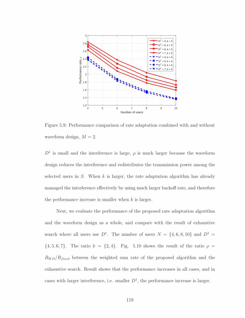
4 5 6 7 8 9 10

Number of users

1.2

1.4

1.6

1.8

2

2.2

2.4

2.6

2.8

3

Per

form

ance

rat

io ρ

D1 = 4, k = 2

D1 = 5, k = 2

D1 = 6, k = 2

D1 = 7, k = 2

D1 = 4, k = 4

D1 = 5, k = 4

D1 = 6, k = 4

D1 = 7, k = 4

Figure 5.9: Performance comparison of rate adaptation combined with and without

waveform design, M = 2.

D1 is small and the interference is large, ρ is much larger because the waveform

design reduces the interference and redistributes the transmission power among the

selected users in S. When k is larger, the rate adaptation algorithm has already

managed the interference effectively by using much larger backoff rate, and therefore

the performance increase is smaller when k is larger.

Next, we evaluate the performance of the proposed rate adaptation algorithm

and the waveform design as a whole, and compare with the result of exhaustive

search where all users use D1. The number of users N = {4, 6, 8, 10} and D1 =

{4, 5, 6, 7}. The ratio k = {2, 4}. Fig. 5.10 shows the result of the ratio ρ =

RWD/Rfixed between the weighted sum rate of the proposed algorithm and the

exhaustive search. Result shows that the performance increases in all cases, and in

cases with larger interference, i.e. smaller D1, the performance increase is larger.

119

4 5 6 7 8 9 10

Number of users

1.4

1.6

1.8

2

2.2

2.4

2.6

2.8

3

Per

form

ance

rat

io ρ

D1 = 4, k = 2

D1 = 5, k = 2

D1 = 6, k = 2

D1 = 7, k = 2

D1 = 4, k = 4

D1 = 5, k = 4

D1 = 6, k = 4

D1 = 7, k = 4

Figure 5.10: Performance comparison between fixed D1 and rate adaptation with

waveform design, M = 2.

5.6 Summary

In this chapter, we propose a rate adaptation algorithm to simultaneously

determine the optimal subset of transmitting users and the optimal backoff factors

for users to maximize the weighted sum throughput of a downlink TRDMA system.

The rate maximization problem with minimum SINR constraints is transformed

into an MIQCQP problem which can be solved efficiently with an optimization

solver. In the second part, we propose a waveform design and power allocation

algorithm according to the output of the selected user, the assigned backoff factor

and the SINR constraints of the selected users. Results show that the proposed

algorithm improves both the system throughput and the fairness between the users,

especially in cases when the interference is severe. The performance, efficiency,

and the versatile applicability to different physical layer implementations make the

120

proposed algorithm suitable suitable for the time reversal system.

121

Chapter 6

Conclusions and Future Work

6.1 Conclusions

In the first part of this dissertation, we demonstrated the spatial focusing of

the TR system and proposed a positioning system with 1-inch resolution. Based on

the excellent localization precision, we propose a VCTR system for indoor tracking

by deploying multiple virtual checkpoints within the target area. In the second

part, we focused on the interference management problem for increasing the system

performance. First, we proposed a MAC layer scheduler that maximized the system

weighted sum rate while satisfying the users’ QoS requirement. We then devised a

rate adaptation algorithm that manages the interference by optimally selecting the

backoff factors for the users in the TR system. More specifically, we addressed the

following problems in this dissertation.

In Chapter 2, we proposed a time reversal indoor positioning system by uti-

lizing the unique location-specific characteristic of CIR. We addressed the ill-posed

single-AP indoor localization problem by decomposing it into two well-defined sub-

problems. We solve the first subproblem by building a database that maps the

physical geographical location to its corresponding CIR space, which we call the

122

data collection phase. The second subproblem is to calculate the TRRS between

the estimated CIR from the unknown users with those in the database. We built

a prototype to evaluate the characteristics of the CIR and the performance of the

proposed scheme. Results show that the indoor positioning system prototype is the

first-ever system to achieve 1 to 2 cm accuracy in both line-of-sight and non-line-

of-sight cases using only one pair of transmitter and receiver both equipped with a

single antenna.

In Chapter 3, a novel indoor tracking system based on the virtual checkpoint is

proposed. With the experiment results shown in Chapter 2, we constructed virtual

checkpoints where the CIR information within the checkpoints is collected. The

location of the unknown user can be identified when the user passes through the

virtual checkpoints. We built a CIR collection machine prototype for automated

large-scale CIR information collection with a user-friendly GUI. By collecting the

statistics of the TRRS between the unknown user and the CIRs in the database, we

found the CDF of the TRRS of the cases when the unknown user passes the virtual

checkpoint or not. The clear different in CDF indicates that by selecting a proper

threshold, the proposed tracking system can detect the user passing through the

virtual checkpoint with very low false alarm.

In Chapter 4, we proposed a novel scheduler for the general 5G downlink

system. The scheduler maximizes the system weighted throughput and satisfies

the SINR constraints of the users. The objective and constraints are transformed

into an MIQCQP problem. The proposed scheduler has a linear complexity, as

compared with the exponential complexity of the exhaustive search with only slight

123

performance degradation. We also investigated the impact of imperfect channel

information on the proposed scheduler. We analyzed the Golay sequence based

channel estimation scheme of the TR system and reveal the same channel estimation

error distribution as the massive MIMO system. Experiment results show that the

proposed scheduler is versatile to different physical layer structures and is robust the

channel estimation error. The versatility, robustness, and low complexity make the

proposed scheduler suitable for systems with a massive number of users and strict

scheduling deadlines.

Lastly, in Chapter 5, we proposed a rate adaptation algorithm for a downlink

TRDMA system. The algorithm maximizes the system weighted sum throughput

by simultaneously determining the optimal subset of the transmitting users and the

optimal backoff factors for the users. The rate maximization and the minimum

SINR constraints of the users are transformed into an MIQCQP problem, which

can be solved efficiently. We also proposed a waveform design and power alloca-

tion algorithm based on the selected users, the selected backoff factors, and the

SINR constraints. Results show that the proposed algorithm improves the system

throughput and the fairness between users, especially in cases where the interference

is severe. The proposed algorithm is suitable for TR system deployment based on

the performance, efficiency and the versatile applicability to different physical layer

implementations.

124

6.2 Future Work

To fully develop the TR system and to meet the versatile applications, there

are several open problems and challenges that need to be explored and investigated.

The exploration of these issues not only leads to fruitful research results but also

makes the 5G communication system come true with great IoT applications. In this

dissertation, the TR technology for 5G and IoT application can be further explored

in the following aspects.

First, the RF component consistency across different devices needs to be stud-

ied. The spatial temporal focusing effect of the TR system relies on the precise CIR

information collected from the RF component. Any inconsistencies between the RF

components, such as the receiving beam pattern, oscillator frequency mismatch, RF

gain difference, etc. can significantly reduce the TR system performance. Therefore,

further exploration of the quantification and the evaluation of the RF inconsistency

effect on the TR performance is desirable. These researches lead to solutions to mit-

igate the decrease in performance and play an important role for a fruitful system

design.

Moreover, the CIR information is affected by the objects in the environment.

An environment change such as a chair removed or human activity may change

the CIR information significantly. However, there is no precise model about how

the CIR is affected by a specific object change in the surrounding environment.

The CIR model is important to the VCTR system deployment for that the CIR

change significantly decreases the performance and increases the need to recollect

125

the database. The VCTR system can reduce the frequency of recollecting database

if the CIR can be modeled by some parameters. A deep investigation about CIR

modeling is very helpful for actual implementation of the VCTR system and the TR

system performance in general.

The proposed scheduler assumes perfect synchronization among different users

in a downlink scenario. However, the precise synchronization algorithm for uplink

traffic is not yet explored. The synchronization of the users affects the CIR informa-

tion quality observed by the base station. A little shift in time significantly decreases

the spatial temporal focusing effect of the TR system and increases the interference

between users because of the low-quality CIR information. The synchronization be-

tween users with heterogeneous bandwidth also poses a challenge for the TR system

design, because the granularity in time is different for different users. Some users

may synchronize to a wrong time instant and reduce the system performance.

Lastly, the operation of TR system needs a large bandwidth and it is very likely

that the TR system shares the frequency band with other systems. The existence

of another system in the same band polluted the CIR information and degrades the

TR system performance. Quantification of the performance degradation is needed

for the TR system deployment. On the other hand, noise suppression algorithm

and coexistence strategy are very much desirable in these cases to guarantee the TR

system performance.

126

Bibliography

[1] Cisco visual networking index: Global mobile data traffic forecast update,2015v2020. Technical report, Cisco, 2016.

[2] P. Bahl and V.N. Padmanabhan. RADAR: an in-building RF-based user lo-cation and tracking system. In IEEE Int. Cong. Computer Communications,volume 2, pages 775–784 vol.2, 2000.

[3] C. Chen, Y. Chen, H. Q. Lai, Y. Han, and K. J. R. Liu. High accuracy indoorlocalization: A WiFi-based approach. In IEEE Int. Conf. Acoustics, Speechand Signal Processing, pages 6245–6249, March 2016.

[4] Yan Chen, Feng Han, Yu-Han Yang, Hang Ma, Yi Han, Chunxiao Jiang, Hung-Quoc Lai, D. Claffey, Z. Safar, and K.J.R Liu. Time-reversal wireless paradigmfor green internet of things: An overview. IEEE Internet Things J., 1(1):81–98,Feb 2014.

[5] Yan Chen, Yu-Han Yang, Feng Han, and K.J.R Liu. Time-reversal widebandcommunications. IEEE Signal Process. Lett., 20(12):1219–1222, Dec 2013.

[6] Yin Chen, D. Lymberopoulos, Jie Liu, and B. Priyantha. Indoor localizationusing FM signals. IEEE Trans. Mobile Comput., 12(8):1502–1517, Aug 2013.

[7] Dah-Ming Chiu and Raj Jain. Analysis of the increase and decrease algorithmsfor congestion avoidance in computer networks. Comput. Netw. ISDN Syst.,17(1):1–14, Jun 1989.

[8] H. Dahrouj and W. Yu. Coordinated beamforming for the multicell multi-antenna wireless system. IEEE Trans. Commun., 9(5):1748–1759, May 2010.

[9] J. De Rosny, G. Lerosey, and M. Fink. Theory of electromagnetic time-reversalmirrors. IEEE Trans. Antennas Propag., 58(10):3139–3149, Oct 2010.

[10] Arnaud Derode, Philippe Roux, and Mathias Fink. Robust acoustic time re-versal with high-order multiple scattering. Phys. Rev. Lett., 75:4206–4209, Dec1995.

[11] S. Dierks and Niklas Juenger. Scheduling for massive mimo with few excessantennas. In 20th Int. ITG Workshop Smart Antennas, pages 1–5, March 2016.

[12] G.F. Edelmann, T. Akal, W.S. Hodgkiss, Seongil Kim, W.A. Kuperman, andHee Chun Song. An initial demonstration of underwater acoustic communica-tion using time reversal. IEEE J. Ocean. Eng., 27(3):602–609, Jul 2002.

[13] Chen Feng, W.S.A. Au, S. Valaee, and Zhenhui Tan. Received-signal-strength-based indoor positioning using compressive sensing. IEEE Trans. Mobile Com-put., 11(12):1983–1993, Dec 2012.

127

[14] M. Fink. Time reversal of ultrasonic fields. I. basic principles. IEEE Trans.Ultrason., Ferroelect., Freq. Control, 39(5):555–566, Sept 1992.

[15] M. Fink, C. Prada, F. Wu, and D. Cassereau. Self focusing in inhomogeneousmedia with time reversal acoustic mirrors. In Proc. IEEE Ultrasonics Sympo-sium, pages 681–686 vol.2, Oct 1989.

[16] R.J. Fontana and S.J. Gunderson. Ultra-wideband precision asset locationsystem. In IEEE Conf. Ultra Wideband Systems and Technologies, pages 147–150, May 2002.

[17] M. Golay. Complementary series. IRE Trans. Inf. Theory, 7(2):82–87, Apr1961.

[18] Inc. Gurobi Optimization. Gurobi optimizer reference manual, 2015.

[19] Feng Han and K.J.R Liu. A multiuser TRDMA uplink system with 2D paral-lel interference cancellation. IEEE Trans. Commun., 62(3):1011–1022, March2014.

[20] Feng Han, Yu-Han Yang, Beibei Wang, Yongle Wu, and K.J.R Liu. Time-reversal division multiple access over multi-path channels. IEEE Trans. Com-mun., 60(7):1953–1965, Jul 2012.

[21] Benjamin E. Henty and Daniel D. Stancil. Multipath-enabled super-resolutionfor rf and microwave communication using phase-conjugate arrays. Phys. Rev.Lett., 93:243904, Dec 2004.

[22] Roger A. Horn and Charles R. Johnson, editors. Matrix Analysis. CambridgeUniversity Press, New York, NY, USA, 1986.

[23] Jianwei Huang, V.G. Subramanian, R. Agrawal, and R.A. Berry. Downlinkscheduling and resource allocation for OFDM systems. IEEE Trans. WirelessCommun., 8(1):288–296, Jan 2009.

[24] Y. Huang, C. W. Tan, and B. D. Rao. Joint beamforming and power controlin coordinated multicell: Max-min duality, effective network and large systemtransition. IEEE Trans. Wireless Commun., 12(6):2730–2742, Jun 2013.

[25] Yunye Jin, Wee-Seng Soh, and Wai-Choong Wong. Indoor localization withchannel impulse response based fingerprint and nonparametric regression. IEEETrans. Wireless Commun., 9(3):1120–1127, March 2010.

[26] Jahyoung Koo and Hojung Cha. Localizing WiFi access points using signalstrength. IEEE Commun. Lett., 15(2):187–189, February 2011.

[27] A. Kushki, K.N. Plataniotis, and A.N. Venetsanopoulos. Kernel-based position-ing in wireless local area networks. IEEE Trans. Mobile Comput., 6(6):689–705,June 2007.

128

[28] R. Kwan, C. Leung, and Jie Zhang. Proportional fair multiuser scheduling inLTE. IEEE Signal Process. Lett., 16(6):461–464, Jun 2009.

[29] E. Larsson, O. Edfors, F. Tufvesson, and T. Marzetta. Massive MIMO for nextgeneration wireless systems. IEEE Commun. Mag., 52(2):186–195, Feb 2014.

[30] H. Lee, I. Sohn, D. Kim, and K. B. Lee. Generalized MMSE beamformingfor downlink MIMO systems. In IEEE Int. Conf. Communications, pages 1–6,June 2011.

[31] G. Lerosey, J. De Rosny, A. Tourin, A. Derode, and M. Fink. Time reversal ofwideband microwaves. Appl. Phys. Lett., 88(15):154101–154101–3, Apr 2006.

[32] G. Lerosey, J. de Rosny, A. Tourin, A. Derode, G. Montaldo, and M. Fink. Timereversal of electromagnetic waves. Phys. Rev. Lett., 92:193904, May 2004.

[33] G Lerosey, J De Rosny, A Tourin, A Derode, G Montaldo, and M Fink. Timereversal of electromagnetic waves and telecommunication. Radio Sci., 40(6),2005.

[34] Hui Liu, H. Darabi, P. Banerjee, and Jing Liu. Survey of wireless indoorpositioning techniques and systems. IEEE Trans. Syst., Man, Cybern., PartC: Applications and Reviews, 37(6):1067–1080, Nov 2007.

[35] Q. Liu and C. W. Chen. Joint transceiver beamforming design and powerallocation for multiuser mimo systems. In IEEE Int. Conf. Communications,pages 3867–3871, June 2012.

[36] H. Ma, Y. Han, Y. Chen, Z. Safar, F. Han, and K.J.R. Liu. Handshakingprotocol for time-reversal system. US Patent, 9313020, April 12, 2016.

[37] R. Muharar and J. Evans. Downlink beamforming with transmit-side channelcorrelation: A large system analysis. In IEEE Int. Conf. Communications,pages 1–5, June 2011.

[38] I.H. Naqvi, G. El Zein, G. Lerosey, J. de Rosny, P. Besnier, A. Tourin, andM. Fink. Experimental validation of time reversal ultra wide-band communica-tion system for high data rates. IET Microwaves, Antennas Propag., 4(5):643–650, May 2010.

[39] D.W.K. Ng and R. Schober. Energy-efficient resource allocation in OFDMAsystems with large numbers of base station antennas. In Int. Conf. Communi-cations, pages 5916–5920, Jun 2012.

[40] H. Q. Ngo, E. G. Larsson, and T. L. Marzetta. Energy and spectral efficiency ofvery large multiuser MIMO systems. IEEE Trans. Commun., 61(4):1436–1449,Apr 2013.

129

[41] H. Q. Ngo, M. Matthaiou, and E. G. Larsson. Massive mimo with optimal powerand training duration allocation. IEEE Wireless Commun. Lett., 3(6):605–608,Dec 2014.

[42] Hien Quoc Ngo, E.G. Larsson, and T.L. Marzetta. Massive MU-MIMO down-link TDD systems with linear precoding and downlink pilots. In Annu. AllertonConf. on Communication, Control, and Computing, pages 293–298, Oct 2013.

[43] Dragos Niculescu and Badri Nath. VOR base stations for indoor 802.11 po-sitioning. In Procc 10th Annu. Int. Conf. Mobile Computing and Networking,MobiCom ’04, pages 58–69, New York, NY, USA, 2004. ACM.

[44] Neal Patwari and Sneha K. Kasera. Robust location distinction using temporallink signatures. In Proc. 13th Annu. ACM Int. Conf. Mobile Computing andNetworking, MobiCom ’07, pages 111–122, New York, NY, USA, 2007. ACM.

[45] C. A. Pitz, E. L. O. Batista, and R. Seara. On the joint beamforming and powercontrol in cellular systems: Algorithm and stochastic model. IEEE Trans.Wireless Commun., 13(12):6943–6954, Dec 2014.

[46] A. Pokhariyal, K.I. Pedersen, G. Monghal, I.Z. Kovacs, C. Rosa, T.E. Kolding,and P.E. Mogensen. HARQ aware frequency domain packet scheduler withdifferent degrees of fairness for the UTRAN long term evolution. In VehicularTechnology Conf., pages 2761–2765, Apr 2007.

[47] R.C. Qiu, Chenming Zhou, Nan Guo, and J.Q. Zhang. Time reversal withMISO for ultrawideband communications: Experimental results. IEEE Anten-nas Wireless Propag. Lett., 5(1):269–273, Dec 2006.

[48] Guolin Sun, Jie Chen, Wei Guo, and K.J.R. Liu. Signal processing techniquesin network-aided positioning: a survey of state-of-the-art positioning designs.IEEE Signal Process. Mag., 22(4):12–23, July 2005.

[49] David Tse and Pramod Viswanath. Fundamentals of wireless communication.Cambridge university press, 2005.

[50] Beibei Wang, Yongle Wu, Feng Han, Yu-Han Yang, and K.J.R Liu. Green wire-less communications: A time-reversal paradigm. IEEE J. Sel. Areas Commun.,29(8):1698–1710, September 2011.

[51] X. Wang, P. Zhu, F. C. Zheng, C. Meng, and X. You. Energy-efficient resourceallocation in multi-cell OFDMA systems with imperfect CSI. In Vehicular Tech.Conf., pages 1–5, Sept 2015.

[52] C. Wengerter, J. Ohlhorst, and A.G.E. von Elbwart. Fairness and throughputanalysis for generalized proportional fair frequency scheduling in OFDMA. InVehicular Technology Conf., volume 3, pages 1903–1907, May 2005.

130

[53] L.A. Wolsey. Integer Programming. Wiley Series in Discrete Mathematics andOptimization. Wiley, 1998.

[54] Kaishun Wu, Jiang Xiao, Youwen Yi, Dihu Chen, Xiaonan Luo, and L.M. Ni.CSI-based indoor localization. IEEE Trans. Parallel Distrib. Syst., 24(7):1300–1309, July 2013.

[55] Zhung-Han Wu, Yi Han, Yan Chen, and K.J.R Liu. A time-reversal paradigmfor indoor positioning system. IEEE Veh. Technol. Mag., 64(4):1331–1339, Apr2015.

[56] Jie Xiong and Kyle Jamieson. ArrayTrack: A fine-grained indoor locationsystem. In Proc. 10th USENIX Symp. Networked Systems Design and Imple-mentation, pages 71–84, Lombard, IL, 2013. USENIX.

[57] Q. Xu, Y. Chen, and K. Liu. Combating strong-weak focusing effect in time-reversal uplinks. IEEE Trans. Wireless Commun., 15(1):568 – 580, Jan 2015.

[58] Yu-Han Yang, Beibei Wang, W.S. Lin, and K.J.R Liu. Near-optimal waveformdesign for sum rate optimization in time-reversal multiuser downlink systems.IEEE Trans. Wireless Commun., 12(1):346–357, January 2013.

[59] Haifan Yin, D. Gesbert, and L. Cottatellucci. Dealing with interference indistributed large-scale MIMO systems: A statistical approach. IEEE J. Sel.Topics Signal Process., 8(5):942–953, Oct 2014.

[60] M.A. Youssef, A. Agrawala, and A. Udaya Shankar. WLAN location deter-mination via clustering and probability distributions. In Proc. 1st IEEE Int.Conf. Pervasive Computing and Communications, pages 143–150, March 2003.

[61] Moustafa Youssef and Ashok Agrawala. The Horus WLAN location determina-tion system. In Proc. 3rd Int. Conf. Mobile Systems, Applications, and Services,MobiSys ’05, pages 205–218, New York, NY, USA, 2005. ACM.

[62] Moustafa Youssef, Adel Youssef, Chuck Rieger, Udaya Shankar, and AshokAgrawala. PinPoint: An asynchronous time-based location determination sys-tem. In Proc. 4th Int. Conf. Mobile Systems, Applications and Services, Mo-biSys ’06, pages 165–176, New York, NY, USA, 2006. ACM.

[63] Boris Ia Zeldovich, Nikolai F Pilipetskii, and Vladimir V Shkunov. Principles ofphase conjugation. In Berlin and New York, Springer-Verlag (Springer Seriesin Optical Sciences. Volume 42), 1985, 262 p., volume 42, 1985.

[64] Junxing Zhang, Mohammad H. Firooz, Neal Patwari, and Sneha K. Kasera.Advancing wireless link signatures for location distinction. In Proc. 14th ACMInt. Conf. Mobile Computing and Networking, MobiCom ’08, pages 26–37, NewYork, NY, USA, 2008. ACM.

131

[65] Q. Zhang, S. Jin, M. McKay, D. Morales-Jimenez, and H. Zhu. Power allocationschemes for multicell massive MIMO systems. IEEE Trans. Wireless Commun.,14(11):5941–5955, Nov 2015.

[66] Yilin Zhao. Standardization of mobile phone positioning for 3G systems. IEEECommun. Mag., 40(7):108–116, Jul 2002.

132