Real-Time Simulation of Global IlluminationUsing Dire t Radian e MappingThesis byJeppe Revall FrisvadRasmus Revall Frisvad

Supervisors:Niels Jørgen ChristensenPeter FalsterInformati s and Mathemati al ModelingIMM, Te hni al University of Denmark,Kgs. Lyngby, Denmark2nd November 2004

ii

Abstra tThis report presents our master's thesis on global illumination and real-time omputer graphi s written at the Te hni al University of Denmark. Thethesis has two obje tives. First obje tive is to identify and study di�erenttraditional methods for the two omputer graphi s �elds alled photorealisti rendering and real-time graphi s. Following this study in known methodswe introdu e some of our own ideas for improvements on, or onstru tionof, global illumination e�e ts in real-time. One idea was hosen for a moredetailed investigation. We have named the method ontained within thisparti ular idea �Dire t Radian e Mapping� (DRM) and it is mainly a methodfor real-time simulation of di�usely re�e ted indire t illumination. DRM isimplemented and ompared to other methods, whi h are able to simulate thesame visual e�e ts. Capabilities, drawba ks, advantages, and disadvantagesof the method are dis ussed on this ba kground.The se ond obje tive is to investigate the work �ow that is ne essaryif we want to reate a s ene using a modeling tool and move that s eneto an appli ation that an render global illumination e�e ts in real-time.The idea is to put together the fundamental tools needed if the results ofthis report were to be useful for reation of a ommer ial dynami real-time appli ation su h as an ar hite tural previewer or a omputer game.To meet this obje tive we have studied the modeling appli ation Blenderand provided the report with an introdu tion to its usage. Through exportand import s ripts we are able to reate s enes in Blender and use them fordemonstration purposes in a separate Windows appli ation.Keywords: Computer graphi s, radiometry, light transport, lo al illumina-tion, global illumination, ray tra ing, photon mapping, real-time rendering,modeling, Blender, dire t radian e mapping.

iv

ResuméDenne rapport præsenterer vores eksamensprokekt ved Danmarks TekniskeUniversitet, som omhandler global illumination og realtids omputer gra�k.Projektet har to formål. Det første er at identi� ere og studere forskellige tra-ditionelle metoder inden for fotorealistisk rendering og realtids gra�k. Efterdette studie i kendte metoder, vil vi introdu ere nogle af vores egne idéer tilkonstruktion af globale illuminations e�ekter i realtid. Én idé er udvalgt tilen mere detaljeret gennemgang. Vi har valgt at kalde denne metode �Dire tRadian e Mapping� (DRM, kortlægning af direkte radians). Metoden brugesprimært til simulation af di�ust re�ekteret indirekte illumination. DRM erimplementeret og sammenlignet med andre metoder, der også kan simulerelignende visuelle e�ekter. Egenskaber, manglende egenskaber, fordele ogulemper vil blive diskuteret på baggrund af denne sammenligning.Det andet formål er at undersøge det arbejdsforløb, der er nødvendigt forat skabe en s ene vha. et modelleringsværktøj. Modellen skal kunne overførestil et program, som er i stand til at rendere globale illuminations e�ekter irealtid. Idéen er at sammenføre de værktøjer der skal bruges for at skabe enkommer iel dynamisk realtids applikation, som f.eks. et omputer spil. Forat imødegå dette formål har vi studeret modelleringsapplikationen Blenderog indsat en tutorial i rapporten. Gennem export/import s ripts er vi i standtil at modellere s ener i Blender og bruge dem til demonstrationsformål i enseperat Windows applikation.

vi

Prefa eThis thesis is written by Jeppe Revall Frisvad and Rasmus Revall Frisvadin partial ful�llment of the M.S . degree at the te hni al university of Den-mark (DTU). The work was ondu ted from February to September 2004.Supervisors of the proje t were Niels Jørgen Christensen, Asso iate Professorat institute of Informati s and Mathemati al Modeling, and Peter Falster,Asso iate Professor also at the institute of Informati s and Mathemati alModeling (IMM), DTU.The subje t of this thesis is simulation of photorealisti rendering inreal-time. Some modeling of three dimensional s enes will be addressed aswell. The reader should understand the most basi on epts of rendering in omputer graphi s.An a ompanying CD-ROM ontaining developed software, sour e ode,models, and other material related to this thesis has been atta hed in ap-pendix A. All programming and modeling tools used for this thesis are freeof harge and most of them are also open sour e proje ts.

s991020 Jeppe Revall Frisvad ____________________s973867 Rasmus Revall Frisvad ____________________

viii

A knowledgementsIn alphabeti al order, thanks to: Philippe Bekaert for answering questionsof mathemati al nature. Andreas Bærentzen for larifying dis ussions. NielsJørgen Christensen for being supervisor of this proje t, and for pointing outimportant issues in many di�erent ontexts. Peter Falster for supervision,en ouragement, and good dis ussions on ore issues as well as peripheri aldetails. Mikkel Gjøl for hints, ritique and onversations along the way.Bjarke Ja obsen for good hints. Henrik Wann Jensen for on�rmation of ourbelieves with respe t to a few un ertainties. Christian Lange, in parti ular,for onstru tive reviews of our early drafts. Bent Dalgaard Larsen for goodhints and onstru tive ritique along the way. Kasper Høj Nielsen for en- ouraging omments now and then. Per Slotsbo for helpful remarks duringthe beginning of the proje t. Also thanks to the Computer Graphi s andImage Analysis Lun h Club for good ompany at lun h time. Thanks to ourparents for always being there and last but not least thanks to Moni a andIben for good support and for oping with our absen e at late hours.

x

Contents1 Introdu tion 11.1 Ba kground . . . . . . . . . . . . . . . . . . . . . . . . . . . . 51.2 Report stru ture . . . . . . . . . . . . . . . . . . . . . . . . . 5I Real-Time Rendering versus Realisti Image Synthesis 92 The Building Blo ks of Computer Graphi s 132.1 An Array-Based Math Engine . . . . . . . . . . . . . . . . . . 152.2 Polygonal Geometry . . . . . . . . . . . . . . . . . . . . . . . 212.3 The Virtual S ene . . . . . . . . . . . . . . . . . . . . . . . . 232.4 Hidden Surfa e Removal . . . . . . . . . . . . . . . . . . . . . 292.5 S ene Graphs and Spatial Data Stru tures . . . . . . . . . . . 323 The Mathemati al Model of Illumination 353.1 Opti al Radiation . . . . . . . . . . . . . . . . . . . . . . . . . 373.2 Radiometry . . . . . . . . . . . . . . . . . . . . . . . . . . . . 433.3 Photometry . . . . . . . . . . . . . . . . . . . . . . . . . . . . 523.4 Light S attering . . . . . . . . . . . . . . . . . . . . . . . . . . 543.5 The Rendering Equation . . . . . . . . . . . . . . . . . . . . . 663.6 Light Transport . . . . . . . . . . . . . . . . . . . . . . . . . . 713.7 Lo al vs. Global Illumination . . . . . . . . . . . . . . . . . . 763.8 Solving Re ursive Integrals . . . . . . . . . . . . . . . . . . . 774 Traditional Approa hes to Realisti Image Synthesis 794.1 Radiosity . . . . . . . . . . . . . . . . . . . . . . . . . . . . . 814.2 Ray Tra ing . . . . . . . . . . . . . . . . . . . . . . . . . . . . 894.3 Monte Carlo Ray Tra ing . . . . . . . . . . . . . . . . . . . . 1014.4 Photon Mapping . . . . . . . . . . . . . . . . . . . . . . . . . 1045 Traditional Approa hes to Real-Time Rendering 1135.1 The Graphi s Rendering Pipeline . . . . . . . . . . . . . . . . 1145.2 Lighting and Shading . . . . . . . . . . . . . . . . . . . . . . . 1205.3 Texture Mapping . . . . . . . . . . . . . . . . . . . . . . . . . 123

xii CONTENTS6 Approximating the Rendering Equation in Real-Time 1276.1 Sten iled Shadow Volumes . . . . . . . . . . . . . . . . . . . . 1286.2 Planar Re�e tions Using the Sten il Bu�er . . . . . . . . . . . 1326.3 Cube Environment Mapping . . . . . . . . . . . . . . . . . . . 1356.4 Real-Time Causti s . . . . . . . . . . . . . . . . . . . . . . . . 1386.5 Complex BRDFs . . . . . . . . . . . . . . . . . . . . . . . . . 1396.6 Light Mapping . . . . . . . . . . . . . . . . . . . . . . . . . . 1406.7 Real-Time Photon Mapping Simulation . . . . . . . . . . . . 1416.8 Pre- omputed Radian e Transfer . . . . . . . . . . . . . . . . 1436.9 Environment Map Rendering . . . . . . . . . . . . . . . . . . 144II Modeling Contents 1477 Modeling 3D S enes 1518 Visual Appearan e 1598.1 Colors and Human Per eption . . . . . . . . . . . . . . . . . . 1608.2 Material Parameters . . . . . . . . . . . . . . . . . . . . . . . 1648.3 Textures . . . . . . . . . . . . . . . . . . . . . . . . . . . . . . 1679 Making Things Come Alive 1699.1 Transformation . . . . . . . . . . . . . . . . . . . . . . . . . . 1709.2 Animation and Motion Control . . . . . . . . . . . . . . . . . 1739.3 Intera tive Control . . . . . . . . . . . . . . . . . . . . . . . . 17510 Modeling in Blender r 17910.1 Blender Navigation . . . . . . . . . . . . . . . . . . . . . . . . 18010.2 Modeling in Blender . . . . . . . . . . . . . . . . . . . . . . . 18510.3 Material Settings in Blender . . . . . . . . . . . . . . . . . . . 19310.4 Blender Animation . . . . . . . . . . . . . . . . . . . . . . . . 19810.5 Export S ripts and Import Libraries . . . . . . . . . . . . . . 20710.6 Additional Blender Features . . . . . . . . . . . . . . . . . . . 209III Ideas, Results, and Experiments 21111 Ideas 21511.1 Angular Visibility Between AABBs . . . . . . . . . . . . . . . 21711.2 Topologi al Network . . . . . . . . . . . . . . . . . . . . . . . 22011.3 Displa ement Mapping . . . . . . . . . . . . . . . . . . . . . . 22111.4 Multi-Agent Global Illumination . . . . . . . . . . . . . . . . 22411.5 Obje t Atmosphere . . . . . . . . . . . . . . . . . . . . . . . . 22511.6 Line-of-Sight Algorithm . . . . . . . . . . . . . . . . . . . . . 22511.7 First Interse tion in Hardware . . . . . . . . . . . . . . . . . . 227

CONTENTS xiii11.8 Single Pixel Images . . . . . . . . . . . . . . . . . . . . . . . . 22912 Dire t Radian e Mapping 23112.1 The Con ept . . . . . . . . . . . . . . . . . . . . . . . . . . . 23212.2 The Resulting Method . . . . . . . . . . . . . . . . . . . . . . 23612.3 Abilities and Limitations . . . . . . . . . . . . . . . . . . . . . 25012.4 Comparison . . . . . . . . . . . . . . . . . . . . . . . . . . . . 25513 Other Implemented Rendering Methods 26113.1 Photorealisti Rendering Methods . . . . . . . . . . . . . . . . 26213.2 Other Real-Time Rendering Methods . . . . . . . . . . . . . . 26414 Graphi al User Interfa e 26914.1 Test S enes . . . . . . . . . . . . . . . . . . . . . . . . . . . . 27014.2 JR Viewer . . . . . . . . . . . . . . . . . . . . . . . . . . . . . 27215 Implementation 28315.1 Program Stru ture . . . . . . . . . . . . . . . . . . . . . . . . 28415.2 Status Options . . . . . . . . . . . . . . . . . . . . . . . . . . 28615.3 Render Options . . . . . . . . . . . . . . . . . . . . . . . . . . 28715.4 S ene Options . . . . . . . . . . . . . . . . . . . . . . . . . . . 28915.5 The Render Engine . . . . . . . . . . . . . . . . . . . . . . . . 291IV Con lusions 29516 Dis ussion 29716.1 Future experiments . . . . . . . . . . . . . . . . . . . . . . . . 29816.2 Appli ability . . . . . . . . . . . . . . . . . . . . . . . . . . . 30117 Con lusion 303A Contents of Atta hed CD-ROM 307B Histori al Remarks 309C Stru ture of Sour e Files and Libraries 315

xiv CONTENTS

Chapter 1Introdu tion

Any su� iently advan ed te hnology is indistinguishable from magi .Arthur C. Clarke (1962): Pro�les of the Future: An Inquiryinto the Limits of the PossibleClarke's Third Law

2 Introdu tionThrough some de ades now people have tried to generate omputer graphi sthat ould repli ate s eneries from real life. Today they have almost rea hedtheir goal. We see movies with omputer animated s enes that are trulydi� ult to distinguish from real life. Soon even experts will �nd it hard, ifnot impossible, to tell whether or not a s ene is taken with a real amera or reated by an animator in a studio. This thesis on erns the fundamentaltheory and methods behind the making of syntheti images.The reation of realisti omputer graphi s images is a heavy omputa-tional pro ess, and it an take a long time to reate small movie s enes evenusing the most powerful omputers. The art of reating syntheti imagesrepli ating the real world very mu h depends on the ability to simulate howlight intera ts with its surroundings. This intera tion is referred to as illu-mination. Throughout this proje t we will dis uss two kinds of illumination;lo al and global. Lo al illumination means that the shade of ea h point in as ene is based solely on the dire tions towards the light sour es and the di-re tion towards the eye point (or amera position). Global illumination alsotakes into a ount the geometry surrounding ea h point in whi h the shadeis to be determined. This has the e�e t that global illumination in ludessu h e�e ts as shadows, re�e tions, refra tions, austi s, olor bleeding, andtranslu en y. The pri e is, however, high. Global illumination is a omputa-tionally expensive model and therefore the methods proposed to simulate itare usually not onsidered in the ontext of real-time graphi s. Contrariwisemany di�erent approa hes have been employed in order to reate visual ef-fe ts similar to global illumination e�e ts in an otherwise lo al illuminationmodel.To a hieve perfe t realism it is lear that global illumination must beintrodu ed or at least a simulation of the e�e ts resulting from global illumi-nation. Sometimes we have plenty of time to generate our image but thereare situations where we are very short on time. Situations like this are foundin dynami omputer appli ations as for example omputer games. In su happli ations it is impossible to foresee every user intera tion, hen e, imagesmust be generated on the �y. The al ulations must be arried out so fastthat the user does not register ea h new pi ture. The pro ess of generat-ing images fast enough for the human eye not to register is referred to asreal-time illumination. In real-time omputer graphi s we often use lo alillumination methods as these traditionally are the only ones that an be al ulated at su� ient speed.The making of syntheti (2-dimensional) images from a three-dimensionalrepresentation (or model) by ombination of lighting, texturing, and geome-try is in omputer graphi s referred to as rendering. The following is a gooddes ription of what it takes for a rendering method to be alled `real-time'[2, p. 1℄:The rate at whi h images are displayed is measured in frames per

3se ond (fps) or Hertz (Hz). At one frame per se ond, there is littlesense of intera tivity; the user is painfully aware of the arrival ofea h new image. At around 6 fps, a sense of intera tivity startsto grow. An appli ation displaying 15 fps is ertainly real-time;the user fo uses on a tion and rea tion. There is a useful limit,however. From about 72 fps and up, di�eren es in the displayrate are e�e tively indete table.It is our intension and the �rst obje tive of this thesis to explore how lose we an bring realisti image synthesis to real-time exe ution rates.As real-time omputer graphi s and realisti image synthesis are twodi�erent bran hes of omputer graphi s we have hosen to start at ea hend and move them slowly in the dire tion of ea h other in the �rm beliefthat we an make them meet somewhere mid-way. We know, however, that ompromises must be taken both with respe t to real-time (72 fps) andrealism, otherwise this obje tive will not be met.Sin e we start at both ends of a long rope stret hing the distan e betweenthe global illumination and real-time rendering we must start out having abasi implementation in both amps. First we must have a basi real-timerenderer as seen in most video games today. This is a hieved using thestandard tools available in a 3D graphi s library su h as OpenGL. Se ondwe must have a de ent renderer simulating global illumination. We have hosen to let this global illumination method be based on the rendering on epts known as ray tra ing and photon mapping.After the emergen e and rapid development of GPUs (Graphi al Pro- essing Units) the prevailing way to implement real-time graphi s is throughhardware. The foundation of 3D omputer graphi s is points and ve torsand the rendering of 3D models onsisting of thousands of triangles results inmillions of al ulations in luding su h mathemati al entities, it is, therefore,evident that an e� ient implementation of ve tor math is ru ial if imagesynthesis is to be brought loser to real-time graphi s. Fortunately the GPUsare developed, in essen e, to pro ess su h al ulations on urrently and ef-� iently. The GPU pro essing is, however, not rea hed easily. GPUs are onstru ted to render triangles in parti ular and the rendering pipeline thata GPU implements is not ne essarily well suited for the di�erent approa hesthat has been found for global illumination.We have studied di�erent aspe ts of global illumination theory to re-ate the foundation whi h we think is ne essary in order to ome up withnew approa hes to global illumination e�e ts in real-time. Several ideas formethods will be dis ussed in the report and the most promising one, whi hwe have hosen to all �Dire t Radian e Mapping�, will be thoroughly exam-ined. Dire t radian e mapping is a method mainly for al ulation of di�uselyre�e ted indire t illumination. Di�use re�e tion o urs when light is equallylikely to be s attered in any dire tion [19℄, this happens when the s attering

4 Introdu tionmaterial looks rather dull. Oppositely spe ular surfa es (su h as mirrorsand glass) re�e t (and refra t) light losely around a parti ular dire tion.Surfa es that have material properties in-between di�use and spe ular are alled glossy. When light has s attered around in a s ene multiple times onarbitrary surfa es (be they di�use, glossy, or spe ular), it is alled indire tillumination. If the indire t illumination has s attered on di�use surfa esat least twi e before rea hing the eye, it is alled di�usely re�e ted indire tillumination. As other approa hes for reating di�usely re�e ted indire tillumination in real-time already exists, we will ompare our method withthese. Some methods only treat perfe tly di�use surfa es (a hypotheti almaterial that s atters light uniformly in all dire tions), su h surfa es areoften referred to as Lambertian surfa es.Coming up with new ideas for real-time global illumination is not easilya omplished and to ome even lose to something useful, most of the existingtheory must be studied thoroughly. With this in mind we have implementedseveral existing global illumination methods both to get familiar with themand to have them later for omparison with real-time results.In s ienti� arti les, papers or reports we often see simple test s enesdemonstrating the treated algorithm or method. This is of ourse suitablefor proof of on ept purposes, but for the method to be appli able in ommer- ial appli ations it must demonstrate e� ien y in more ompli ated setups.As the se ond obje tive of this thesis we want to make a platform for develop-ment of real-time appli ations. We examine not only the rendering methodbut also the entire pro ess from s ene reation to rendering and use of it.This implies that we must be able to model s enes and therefore elementaryuse of a modeling tool is des ribed in this report. We must also des ribeintegration between the modeling tool and our rendering method. In thisthesis we establish a onne tion from s ene reation to rendering of it by ourown methods using free of harge tools only. Finally we have reated a smalldemonstration appli ation, serving the purpose of arranging and presentingall the implemented methods, but also to demonstrate that a s ene an bebuild from s rat h, exported, and then imported in another appli ation.We have hosen to restri t this proje t in a ouple of ways. First we have hosen not to emphasize on the pro ess of software development, rather onthe appli ation of mathemati al tools to solve a omplex problem. Imple-mentation is regarded as a tool for experiments and veri� ation of the ideasthat we put forth. With respe t to omputer graphi s, we have hosen notto dis uss matters of anti-aliasing in detail at any point. We also onsiderreal-time soft shadow methods to be outside the s ope of this report. Noparti ular emphasis will be pla ed on spatial data stru tures for optimiza-tion in this report. We also do not go into parametri urves and surfa esat any point. All these subje ts are left out to save time for other parts ofthe proje t.

1.1 Ba kground 51.1 Ba kgroundPrior to this proje t our knowledge in the �eld of omputer graphi s waslimited to introdu tory ourses. This is re�e ted in the report by someissues being des ribed more omprehensively than perhaps ne essary. Thisshould be regarded as a do umentation of the learning pro ess that we havegone through during this thesis.Other ourses that we have followed may have had an impa t on the out- ome of the proje t as well. We have a ba kground in autonomous agentsand omputational intelligen e, whi h has inspired several of the ideas pre-sented in this report. A prior knowledge of array theory has also been agreat sour e of inspiration.1.2 Report stru tureThe report is divided into four parts. Part I on erns the theoreti al sub-je ts whi h are the foundation of the proje t. In this part we onsider ba-si knowledge in the �eld of global illumination and onstru tion of virtuals enes. Many subje ts are introdu ed sin e they make us able to appre iatethe ideas and on eptions of later parts better. Part II on entrates on s ene reation, that is, reation of ontents for the rendering methods. In here weintrodu e methods for building a dynami omputer s ene, sin e this is whatwe seek to render in real-time. While part I is theoreti ally minded part IIis more pra ti ally minded. Part III presents the ideas that we have omeup with for bringing global illumination loser to real-time rendering, and itgives a thorough des ription of the method we saw as the most promisingof our ideas; dire t radian e mapping. Part III will also present the demon-stration appli ation as well as the test s enes that we have reated using thetools des ribed in part II. Part IV ontains dis ussion and on lusion ofthe thesis.Part IChapter 2 on erns some of the most basi subje ts in omputer graphi s,subje ts that are ommon to all appli ations and rendering methods in 3Dgraphi s. We des ribe how the basi elements in a omputer s ene are setup and we introdu e our math engine, whi h does all al ulations that arenot arried out on the GPU. The math engine builds on array theory, whi his therefore also introdu ed here.Chapter 3 is about the theory behind an illumination model. The hapter des ribes the physi al model of light and how it is transformed into omputer graphi s. In this hapter we des ribe the mathemati al modelwhi h all omputer graphi methods and algorithms seek to simulate or solve.

6 Introdu tionIn other words this is the theory that is the foundation of all illuminationmodels that are used in omputer graphi s.Chapter 4 des ribes traditional approa hes to realisti image synthesis.Here we des ribe some of the most ommonly used global illumination meth-ods: Traditional radiosity, traditional ray tra ing, Monte Carlo ray tra ing,and photon mapping.In hapter 5 we look at rendering from a slightly di�erent angle astraditional methods for real-time rendering are treated here. For that reasonthis hapter will mainly on ern lo al illumination. We will dis uss therasterization pipeline whi h is most ommonly used for real-time renderingand we will take a brief look at textures.In hapter 6 di�erent methods for simulation of global illuminatione�e ts in real-time are presented. Some of the methods presented here willlater be used in ombination with dire t radian e mapping while some of themethods will be used for omparison with dire t radian e mapping.Part IIChapter 7 takes a pra ti al angle on reation of a omputer s ene usingthe theory given in hapter 2. Di�erent more or less a knowledged methodsfor reating 3D obje ts will be introdu ed. The des ription of the methodsuses the free of harge modeling tool alled Blender for examples. This isthe modeling tool that we have hosen for this proje t as a part of the work�ow from s ene reation to rendering that we wish to des ribe.Chapter 8 dis usses the visual appearan e of materials a ording totheir olor and material parameters. In this hapter we seek to take a morepra ti al approa h as ompared to that of part I, sin e the main purpose isto des ribe how materials an be set in a modeling appli ation. Nevertheless,we also need to relate the di�erent on eptions to the theory presented inpart I.In hapter 9 we introdu e methods for reating dynami obje ts in as ene. This is an interesting subje t whi h arises when omputer graphi sare available in real-time. Two di�erent ways of reating dynami obje tsare presented. First, we des ribe how to make animation sequen es for usein our real-time appli ation. Se ondly, we des ribe how user intera tion ande�ne dynami movement of obje ts and amera in a real-time environment.Chapter 10 spe i�es how s ene reation, material settings, and anima-tion of dynami obje ts are arried out in Blender. In this way we providethe basi s needed to build a s ene from s rat h, whi h is a part of the de-velopment platform that we strive at. The hapter also re�e ts the learningpro ess that we have gone through, sin e none of us new Blender beforehand,some of the experien es that we have had may be useful to others.

1.2 Report stru ture 7Part IIIChapter 11 presents di�erent ideas that we have ome up with during theproje t. Those are the ideas that we did not have time to examine in detailduring this thesis. The hapter serves the purpose of inspiration and re�e tsthe pro ess that we went through before rea hing the idea of dire t radian emapping.Dire t radian e mapping is the subje t of hapter 12. Here we des ribethe method in details. The hapter will dis uss abilities, advantages, anddrawba ks of the method. Dire t radian e mapping will also be omparedto the real-time methods providing the same e�e ts whi h were des ribed in hapter 6.In hapter 13 we address other illumination methods that have been im-plemented during the proje t. These are mostly global illumination methodsor real-time methods supplementing dire t radian e mapping.Chapter 14 des ribes our demonstration appli ation. We will give ades ription of the di�erent options that the graphi al user interfa e of theappli ation o�ers. The options all orrespond to methods or visual e�e tsdes ribed elsewhere in the report. Contents and purposes of the di�erenttest s enes will also be des ribed.Chapter 15 presents a number of design diagrams to des ribe the im-plementation behind the demonstration appli ation. We will not des ribeevery fun tion in every �le of the appli ation in detail, but on entrate onthe overall data �ow.Part IVChapter 16 dis usses the out ome of this thesis and the ourse of theproje t. Some additional experiments and future appli abilities will be dis- ussed here as well. Chapter 17 on ludes the report.

8 Introdu tion

Part IReal-Time Rendering versusRealisti Image Synthesis

11In the following hapters we will introdu e the fundamental theory and ter-minology that is ne essary in order to des ribe the relationship betweenphotorealisti rendering and real-time omputer graphi s. The �rst hap-ters dis uss some of the theoreti al and mathemati al subje ts that are thebuilding blo ks of omputer graphi s and realisti image synthesis. The last hapters will dis uss di�erent traditional approa hes to photorealisti as wellas real-time rendering, and some of the latest ombinations of these.The purpose of part I is to provide the basi knowledge of omputergraphi s that is ne essary in order to appre iate the methods and ideas(su h as dire t radian e mapping) presented in part III. Some hapters maybe a bit more omprehensive than needed if they only served the purpose ofmaking the ontents of part III understandable. However, we feel that theinformation provided in the following hapters (espe ially hapter 3) givesvaluable knowledge some of whi h is rarely in luded in modern omputergraphi s text books. Therefore we onsider our analysis of the theoreti alfoundation to be an important part of the learning pro ess that led us to mostof the ideas des ribed in part III. The omprehensiveness of the following hapters also re�e ts a desire to build or implement elements from the bot-tom up, and thereby to get a full understanding of on epts in as many areasas possible. An example is the array-based math engine. For several reasonswe hose to rebuild a previous implementation of a math engine: First of allwe felt that there was a good han e of some minor improvements on ern-ing pro essing speed. Se ondly, it gave us a omplete overview of fun tionsavailable and the apabilities of the engine. If new fun tionality was neededwe ould easily extend the math engine. Furthermore the array-based im-plementation of the math engine bases most operations on a few generalgeometri al operators su h that improvements of those few operators willimprove the performan e of the entire math engine signi� antly.The math engine along with other fundamental mathemati al tools thatare often used in omputer graphi s are presented in hapter 2. The intentionof this hapter is to sum up some of the key tools used in the rest of thereport. The hapter starts with a des ription of the math engine basedon array theory; hen e the on epts of array theory will also be addressedhere. The rest of the hapter sums up basi geometri al and omputationalissues often used throughout the report. All in all it should provide a goodba kground for the rest of the report.Chapter 3 on erns the rendering equation, whi h in some version or an-other is the equation that global illumination methods seek to solve. The hapter treats opti s, opti al radiation, and radiometry whi h are the fun-damentals of the rendering equation. Other areas of resear h that an berelated to omputer graphi s are dis ussed in short (eg. photometry). Forreasons mentioned above hapter 3 digs a bit deeper than perhaps ne essary.After a thorough examination of the basi theories and physi s of light wemove on to the a tual algorithms used in omputer graphi s. Photorealisti

12rendering seek to solve the global illumination model and sin e we would liketo simulate photorealisti rendering in real-time we start out with hapter4, where we des ribe traditional methods for global illumination su h as raytra ing and radiosity. Hybrid methods su h as photon mapping are des ribedand some expansions are addressed shortly.Not only do we want to reate photorealisti e�e ts, we also want themin a real-time s enario. Traditional approa hes to real-time rendering aredes ribed in hapter 5. Most real-time graphi s are based on a lo al illu-mination model rather than a global. The reason is that the al ulationsneeded for lo al illumination are mu h simpler and, hen e, so are the om-putation times. This is ne essary if the illumination of a s ene needs torun in real-time. We will try to des ribe brie�y how real-time graphi s aredone traditionally using rasterization and a lo al illumination model. Eventhough we seek to generate global illumination e�e ts we �nd that mu h ofour �nal implementation has to be based on rasterization in order to run inreal-time. Therefore it is ne essary to des ribe the basi s of rasterization aswell as global illumination te hniques.The last hapter of part I, hapter 6, seeks to ombine global illuminationand real-time rendering by treatment of di�erent visual e�e ts that existin global illumination, but not in lo al illumination, individually. Some ofthe visual e�e ts that have been approa hed using real-time te hniques are:Shadows, re�e tions, refra tions, translu en y, austi s, and olour bleeding.The te hniques for real-time simulation of global illumination e�e ts areplenty: Shadow volumes, environment mapping, light mapping, et . Someof these te hniques are des ribed in hapter 6. Normally methods for real-time global illumination fo us on one of the visual e�e ts, therefore therewill be examples of di�erent approa hes to address di�erent visual e�e ts.In short hapter 6 seeks to give a brief presentation of what others havedone to approa h global illumination in real-time. This is important to us,sin e our own methods do not present a solution for all global illuminatione�e ts and neither does it rule out a ombination with methods presentedby others.

Chapter 2The Building Blo ks ofComputer Graphi s

What are you able to build with your blo ks?Castles and pala es, temples and do ks.Rain may keep raining, and others go roam,But I an be happy and building at home.Robert Louis Stevenson (1850�1894): Blo k Cityfrom �A Child's Garden of Verses and Underwoods�

14 The Building Blo ks of Computer Graphi sIn this hapter we will des ribe some of the basi on epts and mathemat-i al tools that are (or ould have been) used in this proje t. There are noparti ular graphi al methods in this hapter rather the mathemati al foun-dation to build these methods from. Most of the hapter on entrates onbasi ve tor math in a three dimensional world.In se tion 2.1 we will present an array-based math engine that imple-ments the geometri al al ulations and ve tor math that has been used forthe implementation of algorithms that are des ribed in hapters to ome,with the ex eption of al ulations that take pla e on the GPU (Graphi alPro essing Unit). We have hosen to rebuild a ve tor library alled CGLAthat has been implemented by Andreas Bærentzen, and was distributed dur-ing the DTU �Computer Graphi s� ourse (02561). Though we ould haveused CGLA or other implementations of more or less the same fun tions, we hose to make our own implementation inspired by CGLA. As mentionedbefore the reason for starting over is that we get a mu h better understand-ing of what is needed in graphi al al ulations and if some things need tobe hanged or modi�ed we are able to do so faster and easier. Moreover theidea of a math engine based on a few array theoreti operators is appealing.The geometry displayed in 3D omputer graphi s, and espe ially real-time omputer graphi s, often build on polygons. Se tion 2.2 will dis ussways of representing obje ts in a virtual environment su h as a omputers ene. In this proje t we use polygons for obje t representation; hen e, these tion will introdu e how a lever representation of polygons an be puttogether.A 3D virtual s ene is made visible to us on a 2D s reen. In the virtualenvironment this is en losed by a view plane. The position of the view planeis determined by the position of the viewer or eye point, normally representedby a amera. Se tion 2.3 brie�y presents the di�erent elements in a typi alvirtual s ene.Another important issue in omputer graphi s is visibility and ulling,whi h we address in se tion 2.4. A lot of omputations an be saved if theinvisible parts of a s ene are ruled out when rendering. A good idea is tolook loser at how we leave out ba ksides of obje ts not visible to the eye ina s ene. This is normally referred to as ulling.To do graphi s fast it is ne essary to handle the data representing theobje ts of a s ene in a lever way. Se tion 2.5 addresses spatial data stru -tures and s ene graphs, whi h are used to handle the huge amounts of datarepresenting a s ene in a smart way that an speed up pro essing time. Thesubje t of se tion 2.5 will only be treated brie�y, sin e we did not have timeto implement these improvements in our �nal appli ation. However, the se -tion has not been left out entirely sin e spatial data stru tures and s enegraphs ought to be implemented in future versions of our appli ation.

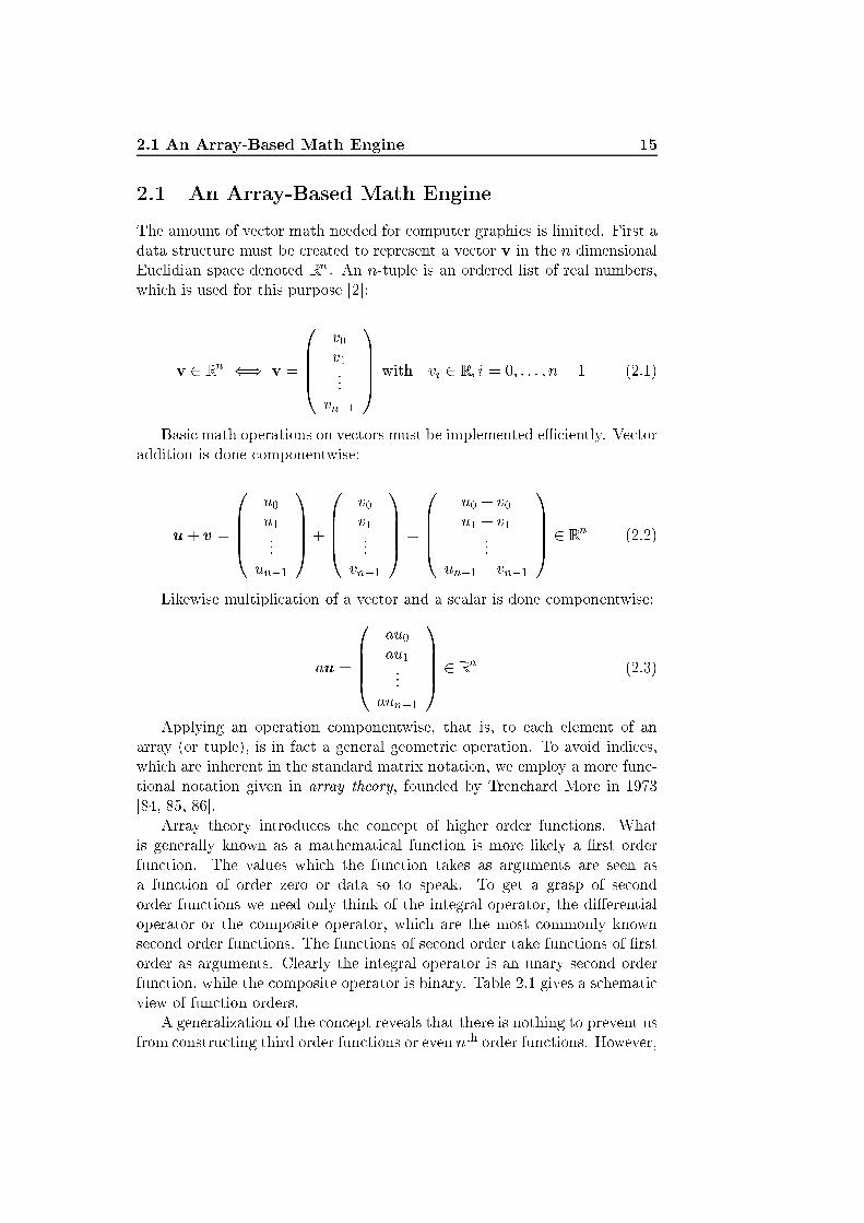
2.1 An Array-Based Math Engine 152.1 An Array-Based Math EngineThe amount of ve tor math needed for omputer graphi s is limited. First adata stru ture must be reated to represent a ve tor v in the n dimensionalEu lidian spa e denoted Rn . An n-tuple is an ordered list of real numbers,whi h is used for this purpose [2℄:v 2 Rn () v = 0BBB� v0v1...vn�1 1CCCA with vi 2 R; i = 0; : : : ; n� 1 (2.1)Basi math operations on ve tors must be implemented e� iently. Ve toraddition is done omponentwise:u+ v = 0BBB� u0u1...un�1 1CCCA+0BBB� v0v1...vn�1 1CCCA =0BBB� u0 + v0u1 + v1...un�1 + vn�1 1CCCA 2 Rn (2.2)Likewise multipli ation of a ve tor and a s alar is done omponentwise:au = 0BBB� au0au1...aun�1 1CCCA 2 Rn (2.3)Applying an operation omponentwise, that is, to ea h element of anarray (or tuple), is in fa t a general geometri operation. To avoid indi es,whi h are inherent in the standard matrix notation, we employ a more fun -tional notation given in array theory, founded by Tren hard More in 1973[84, 85, 86℄.Array theory introdu es the on ept of higher order fun tions. Whatis generally known as a mathemati al fun tion is more likely a �rst orderfun tion. The values whi h the fun tion takes as arguments are seen asa fun tion of order zero or data so to speak. To get a grasp of se ondorder fun tions we need only think of the integral operator, the di�erentialoperator or the omposite operator, whi h are the most ommonly knownse ond order fun tions. The fun tions of se ond order take fun tions of �rstorder as arguments. Clearly the integral operator is an unary se ond orderfun tion, while the omposite operator is binary. Table 2.1 gives a s hemati view of fun tion orders.A generalization of the on ept reveals that there is nothing to prevent usfrom onstru ting third order fun tions or even nth order fun tions. However,

16 The Building Blo ks of Computer Graphi sLogi Mathemati s Array Theory Examples0th order fun tion Value, element Data (box) 1; �; 231st order fun tion Operation Fun tion (gin) +; �; sin2nd order fun tion Operator Transformer (rig) R ;0 ; ÆTable 2.1: A s hemati view of fun tion orders in luding a few examples.sin e even the fun tions of se ond order are quite abstra t and at manyo asions di� ult to grasp, it is even more di� ult to imagine the spe i� use of third order fun tions taking transformers (or se ond order fun tions)as arguments. On the other hand transformers have shown their worth andthe few well known transformers given as examples in table 2.1 are only thetop of the i eberg, so we may yet also �nd a third order fun tion whi h ispra ti ally useful.When applying a fun tion f to a value x the usual notation is f(x)returning a value y being a fun tion of the same order as x. To treat fun tionsof arbitrary order it is important that we an separate the fun tion from itsargument, so that y = f(x) = f (x) = (f x) = f xthis has a meaning when a se ond order fun tion T is introdu ed. Supposewe would like to transform f into a di�erent fun tion a ording to a generalgeometri operation T then g = Tf de�nes a new fun tion g, whi h is thetransformation of f a ording to T , meaning thatg(x) = (T f)(x) = (T f)x = T f xThe equation above indi ates that an array theoreti expression is leftasso iative.De�nition 1 (Left Asso iativity) Expressions having leftasso iativity are analyzed from left to right. Let T be a trans-former, f a fun tion and x a value then the expression T f x�rst evaluates T f and then ombines with x.Left asso iativity rises some questions of interpretation given an arbi-trary expression. The meaning of xf is for example not immediately lear.Consider the expression a + b, here + is a binary fun tion taking two ar-guments: +(a; b). This indi ates that we an interpret a+ as a new unaryfun tion adding the value a to its argument, that is, xf binds x to the �rstargument of the fun tion f :

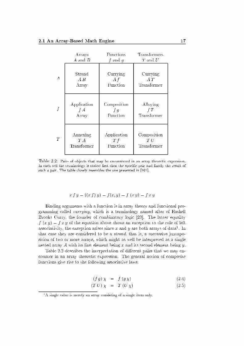
2.1 An Array-Based Math Engine 17Arrays Fun tions TransformersA and B f and g T and UA StrandABArray CurryingAfFun tion CurryingA TTransformerf Appli ationf AArray Compositionf gFun tion Alloyingf TTransformerT AnnexingT ATransformer Appli ationT fFun tion CompositionT UTransformerTable 2.2: Pairs of obje ts that may be en ountered in an array theoreti expression.In ea h ell the terminology is stated �rst then the spe i� pair and �nally the result ofsu h a pair. The table losely resembles the one presented in [101℄.x f y = ((x f) y) = f(x; y) = f (x y) = f x yBinding arguments with a fun tion is in array theory and fun tional pro-gramming alled urrying, whi h is a terminology named after of HaskellBrooks Curry, the founder of ombinatory logi [23℄. The latter equalityf (x y) = f x y of the equation above shows an ex eption to the rule of leftasso iativity, the ex eption arises sin e x and y are both arrays of data1. Inthat ase they are onsidered to be a strand, that is, a su essive juxtapo-sition of two or more arrays, whi h might as well be interpreted as a singlenested array A with its �rst element being x and its se ond element being y.Table 2.2 des ribes the interpretation of di�erent pairs that we may en- ounter in an array theoreti expression. The general notion of ompositefun tions give rise to the following asso iative laws:(f g) � = f (g �) (2.4)(T U) � = T (U �) (2.5)1A single value is merely an array onsisting of a single item only.

18 The Building Blo ks of Computer Graphi swhere � is a fun tion of arbitrary order. Annexing, (2.6), and alloying, (2.7),are also bound by asso iative laws:(T A) = T (A ) (2.6)(f T ) � = f (T �) (2.7)where is an nth order fun tion and n > 0. Finally urrying is also asso ia-tive when the urrying fun tion is of an order greater than one:(A �) � = A (� �) (2.8)where � is an mth order fun tion and m > 1. We will not onsider theimpa t on the asso iative syntax if a third order fun tion was introdu ed.Instead, now that the most basi syntax is in pla e, we an de�ne some ofthe transformers that will ome in handy. First a very basi array theoreti transformer alled EACH2 is introdu ed.De�nition 2 (EACH) Let A be an array of data and let fbe an unary �rst order fun tion, thenEACH f A (2.9)is de�ned as the fun tion f applied to ea h element of thearray A.Sin e an n-tuple is a spe ial ase of an array we an rede�ne multipli a-tion of a ve tor and a s alar, (2.3), asau = EACH (a ?)u (2.10)where ? is used for multipli ation to make sure that it is onfused neitherwith the dot produ t nor the ross produ t.To deal with omponentwise addition we introdu e another transformerfrom array theory alled EACHBOTH.2In array theory transformers are traditionally written in apital letters.

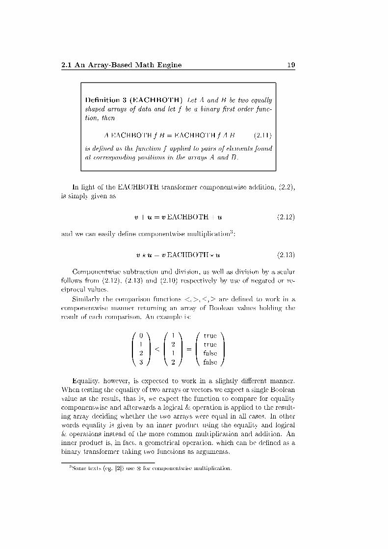
2.1 An Array-Based Math Engine 19De�nition 3 (EACHBOTH) Let A and B be two equallyshaped arrays of data and let f be a binary �rst order fun -tion, thenA EACHBOTH f B = EACHBOTH f A B (2.11)is de�ned as the fun tion f applied to pairs of elements foundat orresponding positions in the arrays A and B.In light of the EACHBOTH transformer omponentwise addition, (2.2),is simply given as v + u = vEACHBOTH+ u (2.12)and we an easily de�ne omponentwise multipli ation3 :v ? u = vEACHBOTH ? u (2.13)Componentwise subtra tion and division, as well as division by a s alarfollows from (2.12), (2.13) and (2.10) respe tively by use of negated or re- ipro al values.Similarly the omparison fun tions <;>;�;� are de�ned to work in a omponentwise manner returning an array of Boolean values holding theresult of ea h omparison. An example is:0BB� 0123 1CCA < 0BB� 1212 1CCA = 0BB� truetruefalsefalse 1CCAEquality, however, is expe ted to work in a slightly di�erent manner.When testing the equality of two arrays or ve tors we expe t a single Booleanvalue as the result, that is, we expe t the fun tion to ompare for equality omponentwise and afterwards a logi al & operation is applied to the result-ing array de iding whether the two arrays were equal in all ases. In otherwords equality is given by an inner produ t using the equality and logi al& operations instead of the more ommon multipli ation and addition. Aninner produ t is, in fa t, a geometri al operation, whi h an be de�ned as abinary transformer taking two fun tions as arguments.3Some texts (eg. [2℄) use for omponentwise multipli ation.

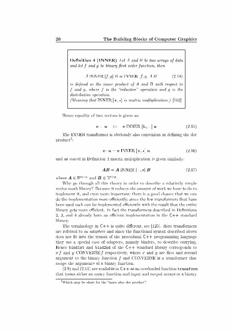
20 The Building Blo ks of Computer Graphi sDe�nition 4 (INNER) Let A and B be two arrays of dataand let f and g be binary �rst order fun tion, thenA INNER [f; g℄ B = INNER [f; g℄ A B (2.14)is de�ned as the inner produ t of A and B with respe t tof and g, where f is the �redu tive� operation and g is thedistributive operation.(Meaning that INNER [+; ?℄ is matrix multipli ation.) [102℄Hen e equality of two ve tors is given as:v = u , v INNER [&;=℄ u (2.15)The INNER transformer is obviously also onvenient in de�ning the dotprodu t4: v � u = v INNER [+; ?℄ u (2.16)and as stated in De�nition 4 matrix multipli ation is given similarly:AB = A INNER [+; ?℄ B (2.17)where A 2 Rm�n and B 2 Rn�p .Why go through all this theory in order to des ribe a relatively simpleve tor math library? Be ause it redu es the amount of work we have to do toimplement it, and even more important; there is a good han e that we ando the implementation more e� iently, sin e the few transformers that havebeen used ea h an be implemented e� iently with the result that the entirelibrary gets more e� ient. In fa t the transformers des ribed in De�nitions2, 3, and 4 already have an e� ient implementation in the C++ standardlibrary.The terminology in C++ is quite di�erent, see [125℄. Here transformersare referred to as adapters and sin e the fun tional syntax des ribed abovedoes not �t into the syntax of the pro edural C++ programming languagethey use a spe ial ase of adapters, namely binders, to des ribe urrying.Hen e bind1st and bind2nd of the C++ standard library orresponds tox f and y CONVERSE f respe tively, where x and y are �rst and se ondargument to the binary fun tion f and CONVERSE is a transformer thatswaps the arguments of a binary fun tion.(2.9) and (2.11) are available in C++ as an overloaded fun tion transformthat treats either an unary fun tion and input and output arrays or a binary4Whi h may be short for the �inner plus dot produ t�.

2.2 Polygonal Geometry 21fun tion and two input and one output array. Likewise (2.14) is implementedas the fun tion inner_produ t. The exa t des ription of these C++ fun -tions are given in [125℄.Moreover the theory that has been des ribed in this se tion gives the fun-damentals needed in order to des ribe fun tional algorithms mathemati ally,hen e we will draw upon it in se tions to ome when we see �t.In the following se tion we will des ribe the basi s of polygons and how 3-dimensional virtual worlds are omposed of polygonal geometry. The subje tof se tion 2.2 may at �rst seem relatively distant from the math engine, buta mathemati al representation and treatment of polygons goes hand in handwith ve tor math.2.2 Polygonal GeometryDe�nition 5 (Polygon) A losed �gure in the plane givenby points p0; p1; : : : ; pn and bounded by line segmentsp0p1; p1p2; : : : ; pn�1pn; pnp0 [98℄.As stated in de�nition 5, a polygon is de�ned as a losed planar �gurebounded by line segments onne ting verti es su h that they en lose oneand only one region. The following list des ribes the properties of a polygon[112, p. 245℄:1. The number of verti es in a polygon equals the number of its sides.2. The number of vertex angles of a polygon equals the number of itssides.3. Ea h side of a polygon is a side of two vertex angles.4. A vertex angle is not a straight angle (6= 180Æ).All polygons an easily be divided into polygons of the lowest order;triangles. Triangles have ertain appealing properties, an example is thattriangulation of all polygons largely will eliminate view-dependent interpo-lation e�e ts [19℄, whi h result from linear interpolation of shade or olorsa ross a polygon. This is exploited by graphi s hardware spe ializing in fasttriangle pro essing. The result is that almost all real-time appli ation basetheir graphi s on triangle meshes, sin e this gives the highest possible reso-lution at a very low rendering time. The level of detail of an obje t dependson the number of triangles used in the mesh and so does the pro essing timefor rendering the obje t.

22 The Building Blo ks of Computer Graphi sFigure 2.1 shows an example of a ylinder represented by polygons. The�gure also shows that polygons an be generated from the onne tion pointsor the edges between them. Polygonal obje ts are often represented by hi-erar hi al data stru tures. Ea h obje t is de�ned by pointers into a list ofsurfa es and ea h surfa e by pointers into a list of verti es. Normally thedata stru tures are optimized, so that ea h point or edge only needs to bestored on e [135℄.

Object Surfaces Polygons Vertices Figure 2.1: An obje t is represented by surfa es, whi h are represented by polygons,whi h are represented by verti es or edges. This �gure is a ombination of �gure 1.1 in[135, p. 5℄ and �gure 2.4 in [134, p. 38℄.In omputer graphi s a vertex is a geometri entity onsisting of a pointin spa e, an asso iated normal, and possibly parametri (u; v)- oordinatesspe ifying the position of the vertex on the surfa e of the obje t whi h it isa part of. The vertex position is represented by three oordinates. Whenmanipulation of these positions is needed, it is evident that the math enginedes ribed in the previous se tion ome in handy.The vertex normal is used for shading. Shading is des ribed in subsequent hapters of this part. Ea h polygon need to have a fa e normal de�ned aswell (the fa e of a polygon is short for its surfa e). The fa e normal is thetrue geometri normal to the plane ontaining the polygon. Fa e normals areused for example in ulling algorithms (se tion 2.4 relates to this subje t).Sometimes it an be appropriate to store the edges between polygons as wellas verti es, sin e they an be useful in shadow al ulations where in prin ipleonly the silhouette of the obje t asting a shadow is interesting. A group ofpolygons forming an obje t is alled a polygon mesh.The biggest drawba k of the polygonal representation is that the detaillevel of obje ts very mu h depends on the number of polygons used for its reation. Sin e all polygons are plane obje ts, urves in an obje t an onlybe ome more pre ise if more polygons are added. Moreover ea h manipu-lation of an obje t must be arried out on ea h polygon present. A highpolygon ount an therefore reate a omputational bottlene k on the CPU

2.3 The Virtual S ene 23(Central Pro essing Unit). An attempt to solve the problem is the rapidly de-veloping GPU (Graphi al Pro essing Unit) whi h is the ore part of moderngraphi s ards. The GPU is on erned mainly with operations on polygons(in parti ular triangles).The number of polygons is not the only issue. GPUs today are so fastthat the problem is a tually not rendering the required amount of triangles,the limitation lies in the amount of data that it is possible to transfer betweenthe CPU and the GPU [134℄.One way to speed up pro essing time is, therefore, to redu e, as mu has possible, the data that need to be transferred. To do this we an eitherredu e the amount of data stored for ea h vertex, or seek to redu e thenumber of verti es. The latter option is typi ally done by exploiting thatmany polygons may share the same verti es or by simpli� ations of the obje tdetails a ording to the needs of a parti ular view (this on ept is oftenreferred to as level of detail, or LOD).Having introdu ed the basi drawing unit that will be used with few ex- eptions throughout this proje t, namely polygons and espe ially triangles,and having presented a way to implement a basi math engine to pro essmathemati al operations on points and ve tors in three dimensions (as de-s ribed in se tion 2.1), it is now time to des ribe the ontents of a traditionalthree-dimensional virtual s ene, whi h is the subje t of the next se tion.2.3 The Virtual S eneWhen wat hing omputer graphi s, either on a TV or on the omputers reen, we are presented with a window into a virtual world. In the photore-alisti ase this world often repli ates our own world. This means that whatwe see is a three dimensional virtual environment.To simulate this in a fairly realisti way we must represent all elementsor obje ts in a s ene in three dimensions. We must also de�ne where wewant to pla e the viewer in the s ene and in whi h dire tion she should belooking. In movies we have a predetermined route for the viewer to follow,whi h means that we know exa tly what will be visible to her at any giventime throughout a sequen e of pi tures. This enables us to pre- al ulate allthe ne essary pi tures, meaning that we in prin iple are able to spend asmu h time as we like for ea h single image, or frame, in a movie sequen e.In a dynami appli ation su h as a omputer game this is, however, not the ase. There is no way to determine the exa t movement of the viewer, thatis, we need to reate ea h image, or frame, on the �y a ording to the urrentlo ation and dire tion of the viewer.To produ e a pi ture we need to keep tra k of all elements in the s eneand most importantly the position of the viewer and the dire tion in whi hshe is looking. Figure 2.2 represents a simple virtual s ene in two dimensions.

24 The Building Blo ks of Computer Graphi sB

C

Viewer

View plane A

Field of View

Figure 2.2: The visible part of the s ene depends on the lo ation of the viewer, the �eldof view (whi h is an angle spe ifying the size of the view plane), and the dire tion, whi hthe viewer is fa ing. In this ase obje ts A and B will be partly visible to the viewer,while obje t C is not visible at all. (Note that obje t B is also only partly visible, sin ethe viewer an not see the ba kside of the sphere, or ir le in the 2D ase.)The view plane is the virtual representation of the s reen and the volumesubtended by the �eld of view en loses the parts of the s ene that be omesvisible when proje ted onto the s reen. This means that the �eld of view isan angle de�ning the visible area.In �gure 2.2 the front of obje t B is fully displayed while the front ofobje t A is only partly visible. Some of the obje t lies behind obje t B anda part of the top orner will be missing sin e it is outside the visible area.To in lude the top orner of obje t A we an either move the eye point upor ba kwards or we ould make the view plane larger by a broadening of the�eld of view. Obje t C is present in the s ene but not inside the visible area,hen e, we an usually leave out C in the al ulations until it be omes visible.By knowing what is visible and what is not, we an save many omputations.This is the subje t of se tion 2.4.The eye point and view plane are normally represented by a amera. Thefun tionality of a amera is omparable to the fun tionality of eye and viewplane; you frame out the part of the world that you want to preserve whenyou hose a motif for your pi ture. What happens outside the pi ture is uto� and forgotten. The simplest model of a amera is the pinhole amera,whi h is shown in �gure 2.3.As in �gure 2.2 the front of obje ts C, D and partly B will be visible on thes reen. Obje ts A and E are both invisible due to the near and far lippingplanes. The lipping planes are in prin iple not a part of the pinhole ameramodel, but are pra ti al espe ially in large s enes. The lipping planes simply

2.3 The Virtual S ene 25

View plane

Pinhole camera

Scene

A

B

C

D

E

Near clipping plane

Far clipping plane

Figure 2.3: In omputer graphi s the eye point and view plane are represented by a amera. This �gure shows the simplest amera model; the pinhole amera and how it aptures a s ene.rule out obje ts that are too lose or too far away. When using near andfar lipping planes, the volume subtended by the �eld of view is ut by twoparallel planes and is, hen e, alled a view frustum. Rasterization, whi h isthe rendering method used for real-time rendering most often, an e�e tively ut away all obje ts that are not partly or fully ontained within the viewfrustum. This is not always possible in photorealisti rendering, sin e lightmay be re�e ted o� obje ts residing outside the view frustum.Normal ameras adjust the size of the view plane by use of di�erent lensespla ed in the hole. Lenses are also used for adjustment of the visible area.The simple pinhole amera has no lens, therefore if the visible area, or the�eld of view, is to be hanged, we need to hange the size of the ameraby hanging hight, breadth, or length and thereby in rease the size of theview plane at the bottom of the amera. This is similar to moving the eyepoint or opening the eye more in �gure 2.2. In this ase a lens is mu h more onvenient. Moreover a lens also lets in more light, whi h makes it preferablein most ases.There is another di�eren e between a pinhole amera and a lens am-era. In the ideal pinhole amera everything is in fo us. This has the e�e tthat omputer graphi s often produ e syntheti images that tend to have an�unnatural� sharpness about them. Lens ameras (and the eye as well) hasa ertain adjustable distan e at whi h the pi tured obje ts will be sharp,meaning that we an only keep fo us on obje ts in a given depth interval,while the pinhole amera has an in�nite depth of �eld [3℄. In real life thelens amera is preferred, sin e it is pra ti al to keep the amera in the samesize and we would like a lot of light to pass through the amera. In om-puter graphi s our amera is arbitrary and we an hange the size and lightwithout any problems. Therefore we prefer to use the mu h simpler pinhole

26 The Building Blo ks of Computer Graphi s

d

Z h

Y

(0, 0) Object size on screen

a

(yp, d)

(-yp, -d)

d

Object

(y, z)

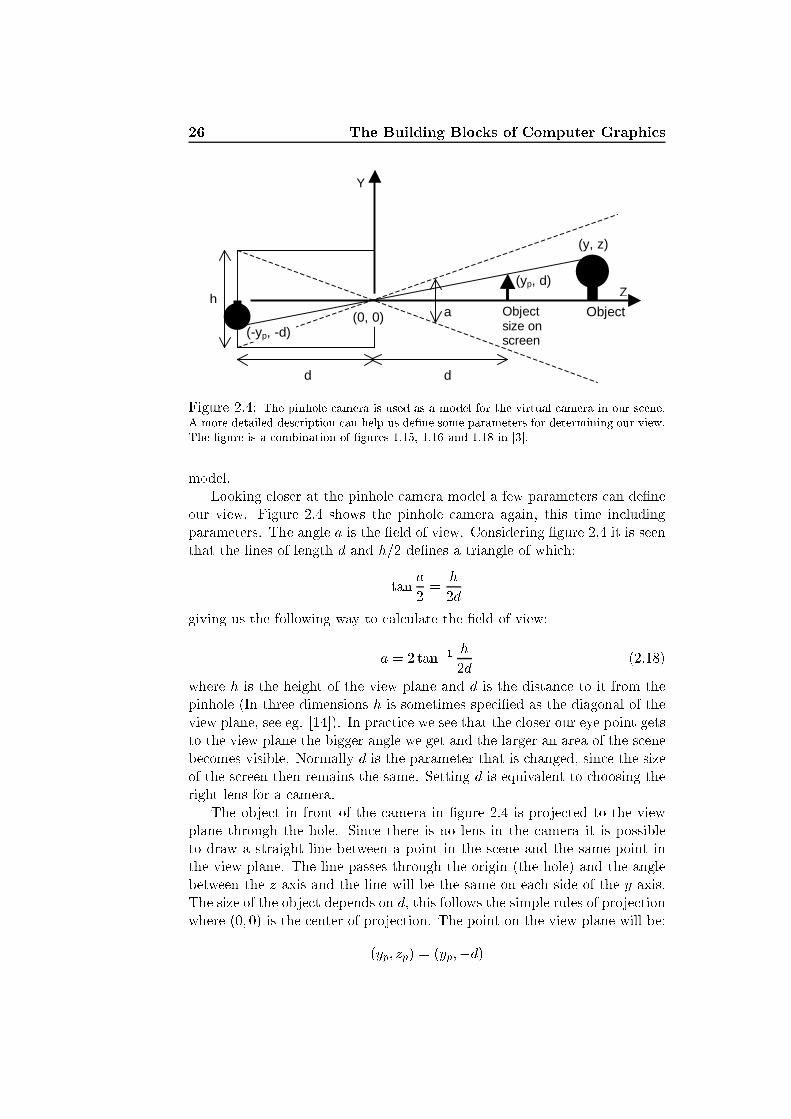
Figure 2.4: The pinhole amera is used as a model for the virtual amera in our s ene.A more detailed des ription an help us de�ne some parameters for determining our view.The �gure is a ombination of �gures 1.15, 1.16 and 1.18 in [3℄.model.Looking loser at the pinhole amera model a few parameters an de�neour view. Figure 2.4 shows the pinhole amera again, this time in ludingparameters. The angle a is the �eld of view. Considering �gure 2.4 it is seenthat the lines of length d and h=2 de�nes a triangle of whi h:tan a2 = h2dgiving us the following way to al ulate the �eld of view:a = 2 tan�1 h2d (2.18)where h is the height of the view plane and d is the distan e to it from thepinhole (In three dimensions h is sometimes spe i�ed as the diagonal of theview plane, see eg. [14℄). In pra ti e we see that the loser our eye point getsto the view plane the bigger angle we get and the larger an area of the s enebe omes visible. Normally d is the parameter that is hanged, sin e the sizeof the s reen then remains the same. Setting d is equivalent to hoosing theright lens for a amera.The obje t in front of the amera in �gure 2.4 is proje ted to the viewplane through the hole. Sin e there is no lens in the amera it is possibleto draw a straight line between a point in the s ene and the same point inthe view plane. The line passes through the origin (the hole) and the anglebetween the z-axis and the line will be the same on ea h side of the y-axis.The size of the obje t depends on d, this follows the simple rules of proje tionwhere (0; 0) is the enter of proje tion. The point on the view plane will be:(yp; zp) = (yp;�d)

2.3 The Virtual S ene 27where yp = � yz=d (2.19)and a similar al ulation an be made for xp:xp = � xz=d (2.20)The resulting image on the view plane, whi h is in ident with the ba k-side of the pinhole amera in �gure 2.4, will as indi ated be turned upsidedown, this is alled ba k proje tion. In order to a hieve front proje tion byproje tion of the image ba k through the origin to a view plane in front ofthe amera (at position z = d), we need merely hange the sign in equations(2.19) and (2.20) [14℄.This se tion has fo used on a virtual s ene with a oordinate system withorigin in the eye point and z-axis along the line of sight. A virtual s ene has,however, several oordinate systems to keep tra k of. The spa e with a o-ordinate system as the one used in this se tion is alled eye (or view) spa e.Besides eye spa e we have a world spa e, whi h has a predetermined oor-dinate system that globally stays the same throughout a rendering session.Obje ts, lights, and the viewer are pla ed in world spa e. Sometimes ea hobje t has its own lo al oordinate system around whi h it was modeled, thisis alled obje t (or model) spa e. When rasterization is used for rendering,the view frustum (in luding its ontents) is transformed into the unit ube,this spa e is alled lip spa e. Last we have the two-dimensional window o-ordinate system whi h is the oordinate system of the s reen or view plane.These spa es ea h have their purpose, and they are des ribed in more detailin hapter 5. In the following we shall shortly des ribe how transformationsare represented mathemati ally in omputer graphi s.Homogenous CoordinatesConsider a point in spa e p = (px; py; pz) and a ve tor in spa e v = (vx; vy; vz).The point des ribes a lo ation, while the ve tor des ribes a dire tion and hasno lo ation. Both are represented by the same three-tuple, whi h makes itdi� ult to distinguish between them with respe t to transformations.We an perform linear transformations, su h as rotations, s alings, andshears, on a three-tuple using 3�3 matri es (this will be des ribed in hapter9). This su� es for transformation of ve tors, sin e they do not have a lo a-tion. If we, however, want to translate a point it is not possible using a 3�3matrix. Be ause of this obvious limitation to the three-tuple representationof points and ve tors omputer graphi s employs a mathemati al tool alledhomogenous oordinates.Suppose we represent ve tors and points using a four-tuple (x; y; z; w).Then, when w 6= 0, homogenous oordinates are given as:

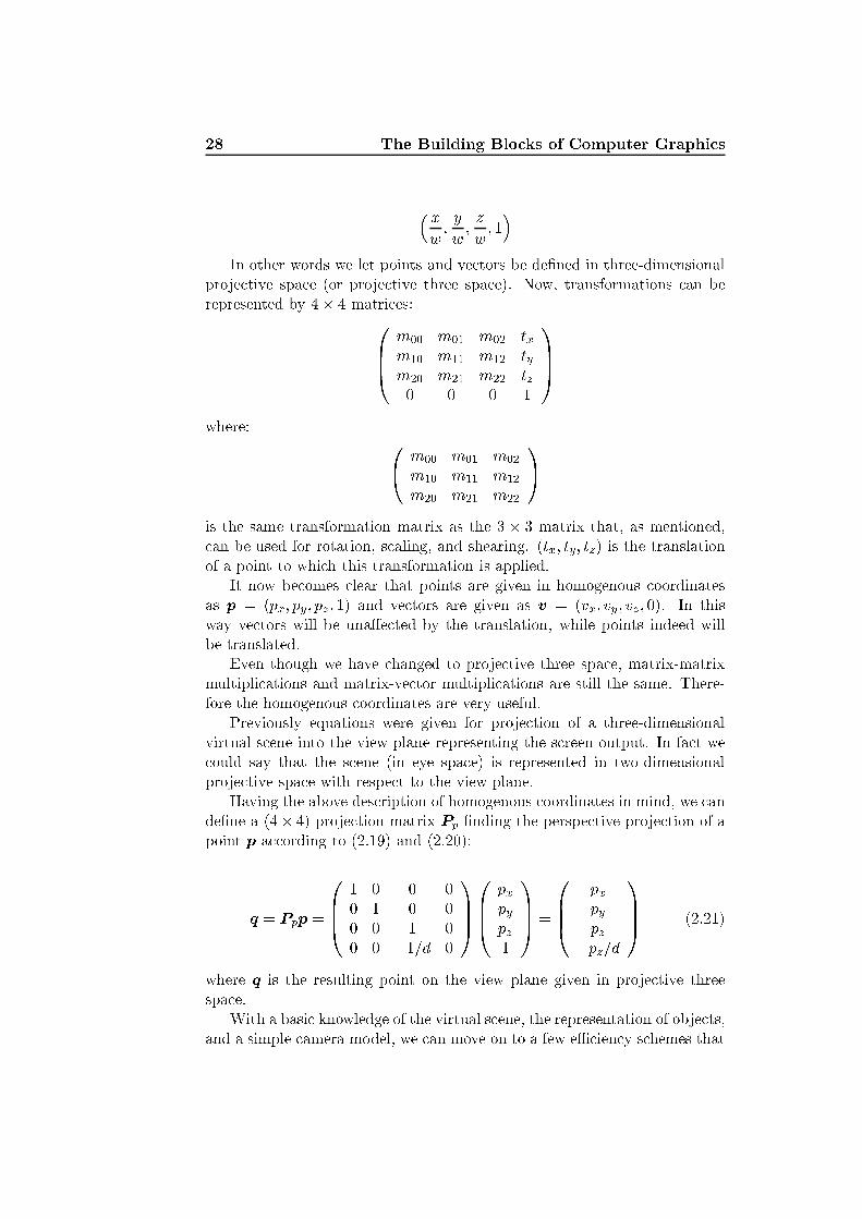
28 The Building Blo ks of Computer Graphi s� xw; yw ; zw ; 1�In other words we let points and ve tors be de�ned in three-dimensionalproje tive spa e (or proje tive three spa e). Now, transformations an berepresented by 4� 4 matri es:0BB� m00 m01 m02 txm10 m11 m12 tym20 m21 m22 tz0 0 0 1 1CCAwhere: 0� m00 m01 m02m10 m11 m12m20 m21 m22 1Ais the same transformation matrix as the 3 � 3 matrix that, as mentioned, an be used for rotation, s aling, and shearing. (tx; ty; tz) is the translationof a point to whi h this transformation is applied.It now be omes lear that points are given in homogenous oordinatesas p = (px; py; pz; 1) and ve tors are given as v = (vx; vy; vz; 0). In thisway ve tors will be una�e ted by the translation, while points indeed willbe translated.Even though we have hanged to proje tive three spa e, matrix-matrixmultipli ations and matrix-ve tor multipli ations are still the same. There-fore the homogenous oordinates are very useful.Previously equations were given for proje tion of a three-dimensionalvirtual s ene into the view plane representing the s reen output. In fa t we ould say that the s ene (in eye spa e) is represented in two-dimensionalproje tive spa e with respe t to the view plane.Having the above des ription of homogenous oordinates in mind, we ande�ne a (4� 4) proje tion matrix Pp �nding the perspe tive proje tion of apoint p a ording to (2.19) and (2.20):q = Ppp = 0BB� 1 0 0 00 1 0 00 0 1 00 0 �1=d 0 1CCA0BB� pxpypz1 1CCA = 0BB� pxpypz�pz=d 1CCA (2.21)where q is the resulting point on the view plane given in proje tive threespa e.With a basi knowledge of the virtual s ene, the representation of obje ts,and a simple amera model, we an move on to a few e� ien y s hemes that

2.4 Hidden Surfa e Removal 29are often useful in omputer graphi s. Se tion 2.4 des ribes how visibility an be exploited and se tion 2.5 shows how spatial data stru tures often anbe an advantage.2.4 Hidden Surfa e RemovalWhen a s ene is rendered there is usually (at least in the ase of lo al illumi-nation) no need to spend unne essary time al ulating lighting and shading onditions for obje t parts that are partly o luded or not visible at all. Theprevious se tion showed how only a part of the s ene is visible to the virtual amera. This se tion will dis uss how to rule out invisible obje ts or partsof obje ts before doing expensive lighting al ulations.There are three steps to go through when removing hidden surfa es. Firstof all we must remove all obje ts outside the visible area, the visible area orresponds to the view frustum, see se tion 2.3. In �gure 2.5 the visiblepart of the s ene is bound by six planes and in a moment we will show howto �nd them. Furthermore we an remove all ba k fa ing surfa es, that is,surfa es with normals pointing away from the viewer and last we an removeall parts of obje ts that lie behind other obje ts in the s ene.

Eye point

Line of sight a

b

Y

Z

X

(-xn, yn, d)

(-xn, -yn, d)

(xn, yn, d)

(xn, -yn, d)

(-xf, yf, e)

(xf, yf, e)

(-xf, -yf, e)

(xf, -yf, e)

d e Figure 2.5: Illustration of the view frustum onstrained by six planes. The view planeis in ident with the near lipping plane. 2a is the height and 2b is the width of the viewplane. d is the distan e from the eye point (residing in the origin sin e we are working ineye spa e) to the near lipping plane, while e is the distan e to the far lipping plane. Then subs ript denotes near, while the f subs ript denotes f ar. The �gure resembles �gure1.9 of [135℄.The six planes bounding the view frustum are referred to as the top,bottom, left, right, near, and far planes. In pra ti e it is normal to pla ethe near lipping plane just in front of the amera so that you an not see

30 The Building Blo ks of Computer Graphi sthrough obje ts. Another pra ti al issue is what to do when the visiblearea ex eeds the far lipping plane, whi h often is the ase when simulatingoutdoor environments. Simply utting when the far lipping plane is rea hed an give unwanted e�e ts, for example obje ts suddenly disappearing oremerging in the horizon (this is alled popping). Fog is a simple atmospheri e�e t that an gradually hide distant obje ts giving a smoother transition[2℄. To de�ne the view frustum we identify ea h plane individually. A plane an be des ribed by a normal n = (�; �; ) and a point in spa e x =(x0; y0; z0): �x+ �y + z + Æ = 0 (2.22)where Æ = �(n � x). The normal an be determined as the ross produ t oftwo linearly independent ve tors, whi h are referred to as the basis of theplane.The left, right, top and bottom planes of the view frustum all have theeye point in ommon. From ea h orner of the view plane a ommon basisve tor for two of those four planes an be found by subtra tion of the eyepoint.The view plane is perpendi ular to the line of sight and follows the z-axisin the eye spa e oordinate system. Therefore the line of sight is a normalfor both the near and the far lipping planes, and a point on the plane isgiven by the distan es d and e as shown in �gure 2.5. Using the line of sightand the basis ve tors de�ned by the orners of the view plane we an de�nean equation for ea h of the six planes bounding our view frustum.Consider a point in eye spa e (xe; ye; ze), for the four points in the near lipping plane ze = d and for the far lipping plane ze = e. Sin e the eyepoint resides in the origin the four basis ve tors given by the orners of theview plane (whi h in this ase is in ident with the near lipping plane) aregiven as: b0 = 0� �xn�ynd 1A =0� �b�ad 1Ab1 = 0� �xnynd 1A =0� �bad 1Ab2 = 0� xnynd 1A =0� bad 1A

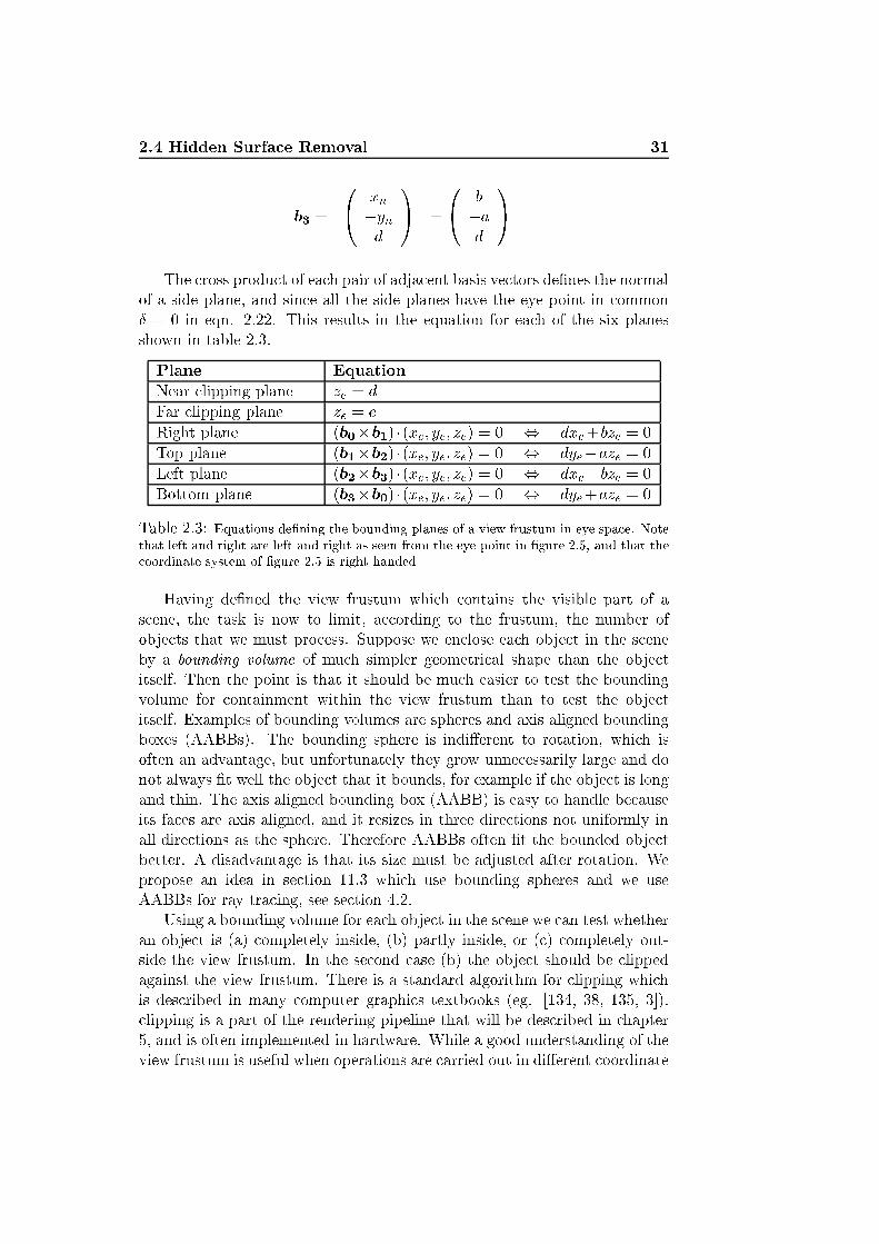
2.4 Hidden Surfa e Removal 31b3 = 0� xn�ynd 1A = 0� b�ad 1AThe ross produ t of ea h pair of adja ent basis ve tors de�nes the normalof a side plane, and sin e all the side planes have the eye point in ommonÆ = 0 in eqn. 2.22. This results in the equation for ea h of the six planesshown in table 2.3.Plane EquationNear lipping plane ze = dFar lipping plane ze = eRight plane (b0�b1) �(xe; ye; ze) = 0 , dxe+bze = 0Top plane (b1�b2) �(xe; ye; ze) = 0 , dye�aze = 0Left plane (b2�b3) �(xe; ye; ze) = 0 , dxe�bze = 0Bottom plane (b3�b0) �(xe; ye; ze) = 0 , dye+aze = 0Table 2.3: Equations de�ning the bounding planes of a view frustum in eye spa e. Notethat left and right are left and right as seen from the eye point in �gure 2.5, and that the oordinate system of �gure 2.5 is right-handedHaving de�ned the view frustum whi h ontains the visible part of as ene, the task is now to limit, a ording to the frustum, the number ofobje ts that we must pro ess. Suppose we en lose ea h obje t in the s eneby a bounding volume of mu h simpler geometri al shape than the obje titself. Then the point is that it should be mu h easier to test the boundingvolume for ontainment within the view frustum than to test the obje titself. Examples of bounding volumes are spheres and axis aligned boundingboxes (AABBs). The bounding sphere is indi�erent to rotation, whi h isoften an advantage, but unfortunately they grow unne essarily large and donot always �t well the obje t that it bounds, for example if the obje t is longand thin. The axis aligned bounding box (AABB) is easy to handle be auseits fa es are axis aligned, and it resizes in three dire tions not uniformly inall dire tions as the sphere. Therefore AABBs often �t the bounded obje tbetter. A disadvantage is that its size must be adjusted after rotation. Wepropose an idea in se tion 11.3 whi h use bounding spheres and we useAABBs for ray tra ing, see se tion 4.2.Using a bounding volume for ea h obje t in the s ene we an test whetheran obje t is (a) ompletely inside, (b) partly inside, or ( ) ompletely out-side the view frustum. In the se ond ase (b) the obje t should be lippedagainst the view frustum. There is a standard algorithm for lipping whi his des ribed in many omputer graphi s textbooks (eg. [134, 38, 135, 3℄). lipping is a part of the rendering pipeline that will be des ribed in hapter5, and is often implemented in hardware. While a good understanding of theview frustum is useful when operations are arried out in di�erent oordinate

32 The Building Blo ks of Computer Graphi ssystems (world spa e, eye spa e, lip spa e, et .), we feel that lipping is apro edure so standardized that there is no reason to repli ate it here.Usually the polygons left by the lipping algorithm for further pro essingare still plenty. To further bring down the number of triangles we an removeall ba k fa ing surfa es. This pro ess is referred to as ba k fa e ulling.Ba k fa e ulling onsists of a simple geometri al test. If we des ribethe line of sight by the dire tional ve tor ! = (!x; !y; !z) and the fa enormal of a polygon as n = (nx; ny; nz), then the dot produ t between thetwo determines whether the polygon is fa ing towards the eye point or awayfrom it. Line of sight is sometimes des ribed as the dire tion from the pointon the surfa e towards the eye point, in that ase visibility is determined as! � n > 0. In eye spa e the test simpli�es to nz > 0.When drawing triangles the fa e normal is often determined as the rossprodu t of the dire tional ve tors given by the �rst two edges drawn. Theresult is that, by onvention, polygons drawn in a ounter lo kwise manner(from the point of view of the eye point) will have a normal pointing towardsthe eye point and will, hen e, be front fa ing.The last and most tri ky part is to remove all obje ts or parts of obje ts overed by other obje ts. This is referred to as o lusion ulling. E� ientalgorithms for o lusion ulling are omplex. The problem is that it is dif-� ult to determine whi h obje ts that are likely to be o luders [134℄. Thesubje t of o lusion ulling will not be addressed in detail in this proje t, afew referen es on the subje t are [2, 134, 50℄.Another way to speed up the pro ess of hoosing visible obje ts for ren-dering is s ene graphs. S ene graphs are often useful in omputer graphi sand they are usually onstru ted using some kind of spatial data stru ture tosplit up the s ene in a sensible way. S ene graphs and spatial data stru tureswill be des ribed brie�y in the following se tion.2.5 S ene Graphs and Spatial Data Stru turesBoth realisti image synthesis and real-time te hniques run into the problemof �unrealisti omputation times� ([135℄) if they hoose a naïve brute for erendering te hnique. The problem is usually the huge amount of trianglesthat must be pro essed in order to display images in the desired quality. Oneway to rule out large parts of a s ene qui kly is by spatial subdivision of thes ene.Spatial data stru tures en ompass data stru tures su h as o trees (andquadtrees), kd-trees, BSP (Binary Spa e Partitioning) trees, bounding vol-ume hierar hies, Voronoi diagrams, et . whi h are useful for spatial subdi-vision of a two- or three-dimensional s ene.The kd-tree is an important part of the rendering te hnique alled photonmapping, see [60, Chap. 6℄. Re ent arti les have, however, tested other

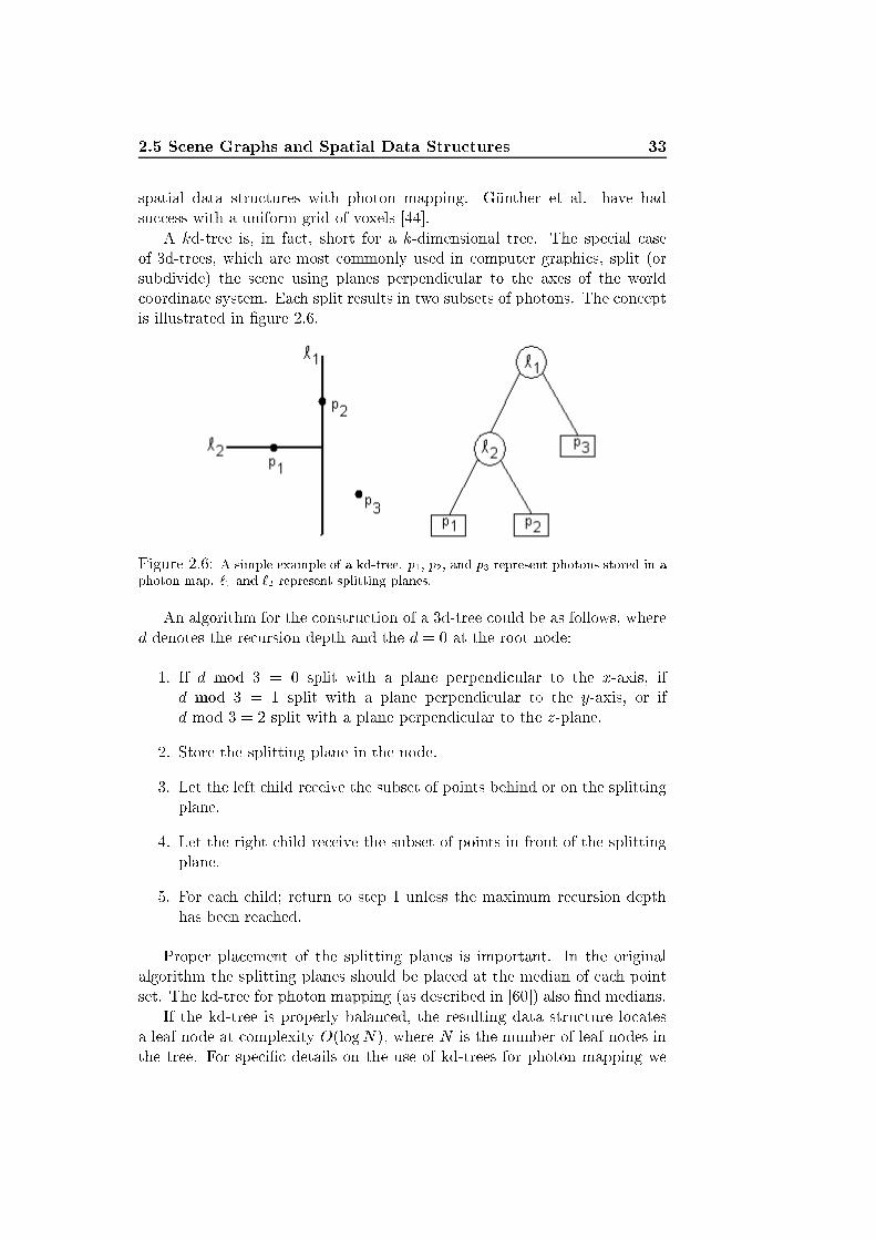
2.5 S ene Graphs and Spatial Data Stru tures 33spatial data stru tures with photon mapping. Günther et al. have hadsu ess with a uniform grid of voxels [44℄.A kd-tree is, in fa t, short for a k-dimensional tree. The spe ial aseof 3d-trees, whi h are most ommonly used in omputer graphi s, split (orsubdivide) the s ene using planes perpendi ular to the axes of the world oordinate system. Ea h split results in two subsets of photons. The on eptis illustrated in �gure 2.6. Figure 2.6: A simple example of a kd-tree. p1, p2, and p3 represent photons stored in aphoton map. `1 and `2 represent splitting planes.An algorithm for the onstru tion of a 3d-tree ould be as follows, whered denotes the re ursion depth and the d = 0 at the root node:1. If d mod 3 = 0 split with a plane perpendi ular to the x-axis, ifd mod 3 = 1 split with a plane perpendi ular to the y-axis, or ifd mod 3 = 2 split with a plane perpendi ular to the z-plane.2. Store the splitting plane in the node.3. Let the left hild re eive the subset of points behind or on the splittingplane.4. Let the right hild re eive the subset of points in front of the splittingplane.5. For ea h hild; return to step 1 unless the maximum re ursion depthhas been rea hed.Proper pla ement of the splitting planes is important. In the originalalgorithm the splitting planes should be pla ed at the median of ea h pointset. The kd-tree for photon mapping (as des ribed in [60℄) also �nd medians.If the kd-tree is properly balan ed, the resulting data stru ture lo atesa leaf node at omplexity O(logN), where N is the number of leaf nodes inthe tree. For spe i� details on the use of kd-trees for photon mapping we

34 The Building Blo ks of Computer Graphi srefer to [60℄, and for further details on the geometri al aspe ts of kd-treesand many other useful spatial data stru tures [25℄ is a good referen e.In addition to the use of kd-trees for photon mapping, spatial data stru -tures have ountless appli abilities in omputer graphi s. A few examplesare: A quad-tree storing obje ts omputed on the �y and used as a fast s enegraph for real-time environments [35℄, o trees, BSP trees, and bounding vol-ume hierar hies for redu tion of ray-triangle interse tions in ray tra ing [135℄(ray-triangle interse tions are des ribed in se tion 4.2), and a quad-tree forshaft o lusion ulling and shadow ray a eleration [117℄. In general spatialdata stru tures are used to a hieve speed-ups whenever the obje ts in a s enehave to be sear hed in one way or another.A s ene graph, as presented in [35℄, is a higher level tree stru ture storingmore than just geometry. Light sour es an be stored in a s ene graph,textures, and transformation matri es as well. When rendering, the treeis traversed in a depth-�rst order and textures, tranformations, and lightsour es an be asso iated with an internal node so that it is only applied tothe subtree of that parti ular node [2℄. When a dynami environment growsin size s ene graphs are indispensable, both to keep tra k of obje ts in thes ene and to speed up rendering. S ene graphs and spatial data stru turesare some of the subje ts that we have hosen not to treat thoroughly in thisproje t. Nevertheless they are quite useful, and they should be studied inthe future if our test s enes grow larger.The drawba k of spatial data stru tures for real-time rendering is thatthey are often quite ostly to onstru t and re- onstru t when things hangedynami ally. This has the result that they must be either very simple havinga reasonable size or they must be pre- omputed.For a truly dynami s ene it is di� ult to pre- ompute all possible ver-sions of spatial data stru ture, not to say impossible if we want, for example,a BSP tree with a single triangle in ea h leaf node. Tiles are therefore oftenused in s enes for real-time rendering and a graph is established and pre- omputed between those, or simple data stru tures (su h as the quad-treementioned before) are omputed on the �y.Unfortunately we have not been able to spare time during this proje tfor a thorough investigation of spatial data stru tures. Most of the s enesthat we have tested have not been su� iently omplex to draw advantageof BSP trees or the like. However, we have developed a simple spatial datastru ture based on solid angles, and used a few other optimization s hemesfor ray tra ing, those will be des ribed in part III.

Chapter 3The Mathemati al Model ofIllumination

So rates: Though vision may be in the eyes and its possessor maytry to use it, and though olor be present, yet without thepresen e of a third thing spe i� ally adapted to this purpose,you are aware that vision will see nothing and the olors willremain invisible.Glau on: What is this [third℄ thing of whi h you speak? he said.So rates: The thing, I said, that you all light.Glau on: You say truly, he replied.Plato (427-347 BC.): The Republi 507e

36 The Mathemati al Model of IlluminationOne purpose of this proje t is to visualize a three-dimensional digital modelas photorealisti images on a omputer s reen, and to make those imagesappear on the s reen at a frequen y that allows intera tive animation of thepi tured elements.These apparently harmless obje tives are, in fa t, quite ontradi tive. Atleast they are ontradi tive on urrent omputer hardware using the urrentvisualization te hniques. Why so? Sin e a perfe t syntheti representationof the real world would onsist of in�nite omplexities. Lu kily we need not ompute an exa t opy of the real world, we an merely fo us on the humanvisual interpretation of the world.What we need is a model that an simulate vision (or photography) as ittakes pla e in real life. What we see is light, hen e, what the mathemati almodel must apture is the intera tion of light with matter, or the illuminationof a s ene. Su h a mathemati al model will be referred to as an illuminationmodel.Simple as it may seem, it is not at all simple to model or even give anexa t explanation of light. Through times many attempts have been made onthe nature of light (see appendix B). Today quantum me hani s explain lighton the parti le level while light in general is onsidered to be ele tromagneti radiation in the infrared, visible, and ultraviolet spe trum. The spe trum ofele tromagneti waves is illustrated in �gure 3.1.In order to onstru t an illumination model we must give a mathemati aldes ription of light. First the propagation of light through di�erent mediamust be modeled. The s ienti� �eld of opti s in ludes a mathemati almodel for the des ription of light propagation. Se tion 3.1 presents somefundamental postulates on erning light propagation on whi h we an buildour illumination model.Next we must introdu e a terminology in our model by whi h we anspe ify how light is measured by the eyes and other opti al dete tors. Ra-diometry o�ers mathemati al de�nitions of the ne essary physi al terms andis des ribed in se tion 3.2.The stri t physi al measures of light do not ne essarily �t the visualresponse of the human eye exposed to light. Photometry is losely relatedto radiometry ex ept for the fa t that it in ludes the visual response of astandard observer in the quanti� ation of light measurements. Photometryis shortly introdu ed in se tion 3.3.Sin e illumination in ludes the intera tion of light with matter we mustin lude in our model how light is re�e ted o�, refra ted through, and ab-sorbed by di�erent materials. These pro esses, and the relation betweenthem, are referred to as light s attering and are modeled in the �eld of heattransfer. Light s attering will be the topi of se tion 3.4.Conse utively the mathemati al des ription of light and how it s atterswill be gathered in an integral equation that we an use for rendering. Therendering equation is des ribed in se tion 3.5.

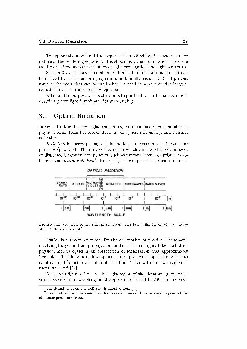
3.1 Opti al Radiation 37To explore the model a little deeper se tion 3.6 will go into the re ursivenature of the rendering equation. It is shown how the illumination of a s ene an be des ribed as re ursive steps of light propagation and light s attering.Se tion 3.7 des ribes some of the di�erent illumination models that anbe derived from the rendering equation, and, �nally, se tion 3.8 will presentsome of the tools that an be used when we need to solve re ursive integralequations su h as the rendering equation.All in all the purpose of this hapter is to put forth a mathemati al modeldes ribing how light illuminates its surroundings.3.1 Opti al RadiationIn order to des ribe how light propagates, we must introdu e a number ofphysi al terms from the broad literature of opti s, radiometry, and thermalradiation.Radiation is energy propagated in the form of ele tromagneti waves orparti les (photons). The range of radiation whi h an be re�e ted, imaged,or dispersed by opti al omponents, su h as mirrors, lenses, or prisms, is re-ferred to as opti al radiation1. Hen e, light is omposed of opti al radiation.

Figure 3.1: Spe trum of ele tromagneti waves. Identi al to �g. 1.1 of [89℄. (Courtesyof F. E. Ni odemus et al.)Opti s is a theory or model for the des ription of physi al phenomenainvolving the generation, propagation, and dete tion of light. Like most otherphysi al models opti s is an abstra tion or idealization that approximates`real life'. The histori al development (see app. B) of opti al models hasresulted in di�erent levels of sophisti ation, �ea h with its own region ofuseful validity� [89℄.As seen in �gure 3.1 the visible light region of the ele tromagneti spe -trum extends from wavelengths of approximately 380 to 780 nanometers.21The de�nition of opti al radiation is adopted from [89℄.2Note that only approximate boundaries exist between the wavelength regions of theele tromagneti spe trum.

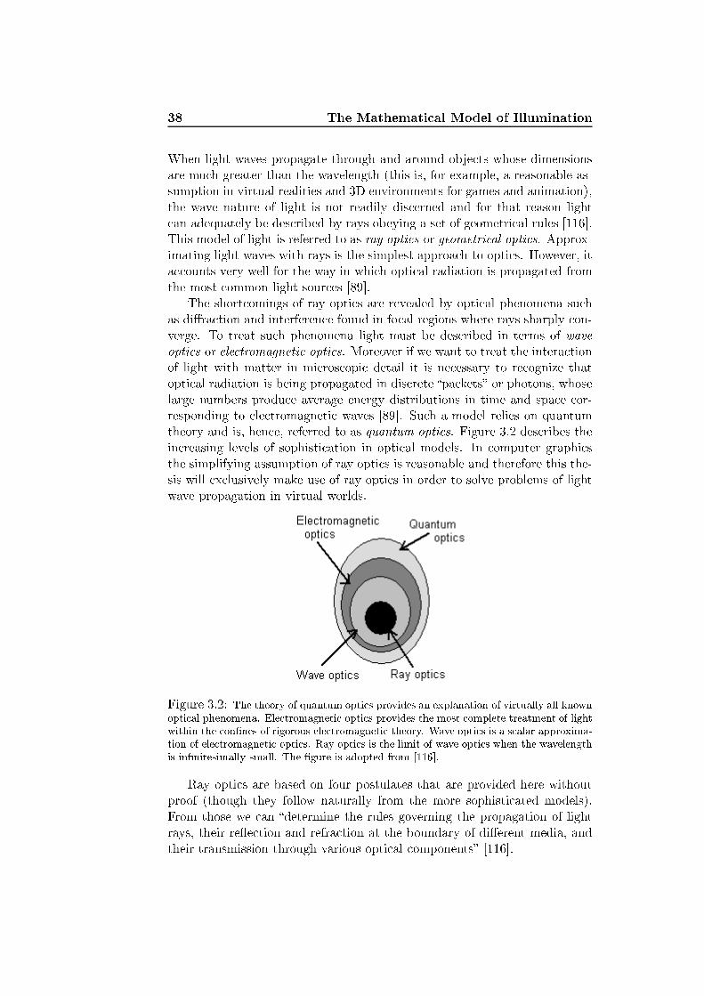
38 The Mathemati al Model of IlluminationWhen light waves propagate through and around obje ts whose dimensionsare mu h greater than the wavelength (this is, for example, a reasonable as-sumption in virtual realities and 3D environments for games and animation),the wave nature of light is not readily dis erned and for that reason light an adequately be des ribed by rays obeying a set of geometri al rules [116℄.This model of light is referred to as ray opti s or geometri al opti s. Approx-imating light waves with rays is the simplest approa h to opti s. However, ita ounts very well for the way in whi h opti al radiation is propagated fromthe most ommon light sour es [89℄.The short omings of ray opti s are revealed by opti al phenomena su has di�ra tion and interferen e found in fo al regions where rays sharply on-verge. To treat su h phenomena light must be des ribed in terms of waveopti s or ele tromagneti opti s. Moreover if we want to treat the intera tionof light with matter in mi ros opi detail it is ne essary to re ognize thatopti al radiation is being propagated in dis rete �pa kets� or photons, whoselarge numbers produ e average energy distributions in time and spa e or-responding to ele tromagneti waves [89℄. Su h a model relies on quantumtheory and is, hen e, referred to as quantum opti s. Figure 3.2 des ribes thein reasing levels of sophisti ation in opti al models. In omputer graphi sthe simplifying assumption of ray opti s is reasonable and therefore this the-sis will ex lusively make use of ray opti s in order to solve problems of lightwave propagation in virtual worlds.

Figure 3.2: The theory of quantum opti s provides an explanation of virtually all knownopti al phenomena. Ele tromagneti opti s provides the most omplete treatment of lightwithin the on�nes of rigorous ele tromagneti theory. Wave opti s is a s alar approxima-tion of ele tromagneti opti s. Ray opti s is the limit of wave opti s when the wavelengthis in�nitesimally small. The �gure is adopted from [116℄.Ray opti s are based on four postulates that are provided here withoutproof (though they follow naturally from the more sophisti ated models).From those we an �determine the rules governing the propagation of lightrays, their re�e tion and refra tion at the boundary of di�erent media, andtheir transmission through various opti al omponents� [116℄.

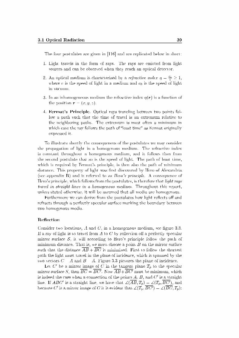
3.1 Opti al Radiation 39The four postulates are given in [116℄ and are repli ated below in short:1. Light travels in the form of rays. The rays are emitted from lightsour es and an be observed when they rea h an opti al dete tor.2. An opti al medium is hara terized by a refra tive index � = 0 � 1,where is the speed of light in a medium and 0 is the speed of lightin va uum.3. In an inhomogeneous medium the refra tive index �(r) is a fun tion ofthe position r = (x; y; z).4. Fermat's Prin iple. Opti al rays traveling between two points fol-low a path su h that the time of travel is an extremum relative tothe neighboring paths. The extremum is most often a minimum inwhi h ase the ray follows the path of �least time� as Fermat originallyexpressed it.To illustrate shortly the onsequen es of the postulates we may onsiderthe propagation of light in a homogenous medium. The refra tive indexis onstant throughout a homogenous medium, and it follows then fromthe se ond postulate that so is the speed of light. The path of least time,whi h is required by Fermat's prin iple, is then also the path of minimumdistan e. This property of light was �rst dis overed by Hero of Alexandria(see appendix B) and is referred to as Hero's prin iple. A onsequen e ofHero's prin iple, whi h follows from the postulates, is therefore that light raystravel in straight lines in a homogenous medium. Throughout this report,unless stated otherwise, it will be assumed that all media are homogenous.Furthermore we an derive from the postulates how light re�e ts o� andrefra ts through a perfe tly spe ular surfa e marking the boundary betweentwo homogenous media.Re�e tionConsider two lo ations, A and C, in a homogenous medium, see �gure 3.3.If a ray of light is to travel from A to C by re�e tion o� a perfe tly spe ularmirror surfa e S, it will a ording to Hero's prin iple follow the path ofminimum distan e. That is, we must hoose a point B on the mirror surfa esu h that the distan e AB + BC is minimized. First to follow the shortestpath the light must travel in the plane of in iden e, whi h is spanned by thetwo ve tors C �A and B �A. Figure 3.3 pi tures the plane of in iden e.Let C 0 be a mirror image of C in the tangent plane Tp to the spe ularmirror surfa e S, then BC = BC 0. Now AB+BC 0 must be minimum, whi his indeed the ase when a onne tion of the points A, B, and C 0 is a straightline. If ABC 0 is a straight line, we have that \(AB; Tp) = \(Tp; BC 0), andbe ause C 0 is a mirror image of C it is evident that \(Tp; BC 0) = \(BC; Tp):

40 The Mathemati al Model of Illumination Figure 3.3: Light traveling in a homogenous medium from a point A re�e ting o� aperfe tly spe ular mirror surfa e S at the point B ending in the point C. Tp is thetangent plane to S, and C0 is the mirror image of C in Tp.\(AB; Tp) = \(Tp; BC 0) = \(BC; Tp) = �Sin e \(AB; Tp) = \(BC; Tp), and sin e the normal n at the surfa epoint B by de�nition is perpendi ular to Tp, it follows that:\(AB;n) = \(n; BC) = � (3.1)whi h states that the angle of re�e tion equals the angle of in iden e ( f. �g.3.3).Let !0 = A�BjjA�Bjj denote the dire tion from whi h the in ident radian eis arriving at the mirror surfa e S, then, a ording to (3.1), the dire tion ofthe re�e ted ray !s an be found as:!s = 2 os �n� !0 = 2(!0 � n)n� !0 (3.2)where � is the angle of in iden e and n is the unit normal at the point ofin iden e. (3.2) is one of many ways to express the law of re�e tion. Anotherenun iation is as given in [116, p. 5℄:The re�e ted ray lies in the plane of in iden e;the angle of re�e tion equals the angle of in iden e. �Refra tionAgain the fourth postulate (Fermat's prin iple) gives means by whi h we anestablish how light refra ts when it passes from one homogenous medium toanother. The di�eren e between the two media is stated as two di�erentindi es of refra tion, �1 and �2 (one for ea h media). In order to �nd thepath that light takes from a point A in the medium of refra tion index �1

3.1 Opti al Radiation 41

Figure 3.4: The path of light when it travels from one homogenous medium to another.to a point B in the medium of refra tion index �2, we must �nd the path ofleast time. Again we need only onsider the plane of in iden e as pi turedin �gure 3.4.Let B be the point of in iden e at the surfa e S, whi h marks the bound-ary between the two di�erent media, and let �1 be the angle of in iden e su hthat: os �1 = !0 � nwhere !0 = A�BjjA�Bjj is the dire tion of in ident light, and n is the unit normalat the point of in iden e. Now, we denote the angle of the refra ted light �2su h that: os �2 = !r � nwhere !r = C�BjjC�Bjj is the dire tion of the refra ted light.The time it takes for light to travel a distan e d equals d= = �d= 0. Thetravel time is thus proportional to the opti al path length, whi h is de�ned as�d. To �nd the path of least time we an, therefore, minimize the opti al pathlength instead of the travel time. Meaning that what we seek to minimize is�1AB + �2BC.Suppose we let the normal n de�ne a v-axis in the plane of in iden e,then B = (u; 0) in (u; v)- oordinates. Furthermore let A = (u1; v1) andC = (u2; v2), then AB =p(u� u1)2 + v21 and BC =p(u2 � u)2 + v22 . Thederivative of the opti al path length is then given as:d(�d)dx = �1 u� u1p(u� u1)2 + v21 + �2 �u2 + up(u2 � u)2 + v22Setting the derivative equal to zero we will dis over an extremum (whi hwill most probably be a minimum) as is required by Fermat's prin iple. Thisyields the following:

42 The Mathemati al Model of Illumination�1 u� u1p(u� u1)2 + v21 = �2 u2 � up(u2 � u)2 + v22or put di�erently: �1 d1AB = �2 d2BCwhere d1 and d2 are the proje tions on the tangent plane of AB and BCrespe tively. Now, Snell's law follows by the trigonometry of a right triangle:�1 sin �1 = �2 sin �2 (3.3)Snell's law gives means by whi h we an �nd a formula for the al ulationof the dire tion of refra tion !r. Suppose t is a unit tangent ve tor to theperfe tly spe ular surfa e S at the point B in the plane of in iden e, andthat n is the unit normal pointing into the medium of refra tion index �1,then the dire tion of the refra ted light is:!r = �n os �2 + t sin �2 (3.4)Suppose the normal n and the dire tion towards the in ident light !0are given. Then the omponent of !0 that is perpendi ular to the normal, isgiven as: !0? = (!0 � n)n� !0while the length of !0? simply is sin �1. An expression for the unit tangentve tor t then follows: t = !0?jj!0?jj = (!0 � n)n� !0sin �1To �nd os �2 of (3.4) we use the property that the angle of in iden ealways lies in the interval [0; �2 ℄, and get that: os �2 =p1� sin2 �2(3.4) then has the following form:!r = �np1� sin2 �2 + sin �2sin �1 ((!0 � n)n� !0)and by Snell's law and a few rearrangements, we retrieve the law of refra tionas it is expressed in many text books (eg. [38, 60, 30℄):

3.2 Radiometry 43!r = sin �2sin �1 ((!0 � n)n� !0)�np1� sin2 �2= �1�2 ((!0 � n)n� !0)� ns1���1�2�2 sin2 �1= �1�2 ((!0 � n)n� !0)� ns1���1�2�2 (1� (!0 � n)2) (3.5)The more textual enun iation of the law of refra tion is given in [116, p.6℄ as: The refra ted ray lies in the plane of in iden e; the angle ofrefra tion �2 is related to the angle of in iden e �1 by Snell's law,�1 sin �1 = �2 sin �2 �Based on the four postulates of ray opti s, it has now been established howlight propagates in homogenous media. The three simple rules are:� Propagation in straight lines� The law of re�e tion� The law of refra tionThe laws of re�e tion and refra tion on erns only perfe tly spe ularmaterial, nevertheless, they are important sin e the re�e tion and refra tionof glossy materials (whi h are materials with properties that lie in-betweenperfe tly spe ular and perfe tly di�use) in general are entered around theperfe t dire tions.Having established the basi properties of light propagation on whi h tobuild our illumination model, we an pro eed to the radiative properties oflight, whi h will allow us a des ription of the light that an be measured atopti al dete tors su h as the eye.3.2 RadiometryWhile opti s on ern the generation, propagation, and dete tion of light,radiometry is the s ien e of ele tromagneti radiation measurement.The basi quantity of radiometry is radian e, L, whi h most losely rep-resents the olors that we see [60℄. Therefore radian e is a very important

44 The Mathemati al Model of Illuminationquantity in omputer graphi s, and radian e is what we must al ulate anddisplay to an observer in order to visualize a 3D model.Te hni ally speaking radian e is the amount of radiant energy arrivingat or departing from an in�nitesimal area per unit time with respe t to agiven dire tion. Meaning that radian e an be used to des ribe the intensityof light at a given point in spa e.Radian e is a third derivative of radiant energy, Q. To give a betterunderstanding of radian e the di�erent derivatives of radiant energy will bedes ribed in the following.Radiant FluxFirst we would like to onsider the �ow of energy rather than isolatedamounts. This is obvious sin e the eyes per ept light waves ontinuouslyrather than on timely intervals. Radiant energy per unit time is alled radi-ant �ux, �: � = dQdt (3.6)When looking at an obje t the eye registers the radiant �ux departing theobje t in the dire tion of the eye. To des ribe a dire tional volume throughwhi h the energy an �ow, we need to introdu e the on ept of a solid angle.Solid AngleIn 2-dimensional spa e the more familiar plane angle, �, is formed at thepoint O� where two straight lines meet, see �gure 3.5a. It is de�ned as thelo us of all dire tions that may be o upied by either line as it is rotatedabout the vertex to bring it into dire tional oin iden e with the other line.Drawing a unit ir le entered atO� the length of the ir ular ar inter eptedby � is a measure of the plane angle.The solid angle is formed at a point O! in 3-dimensional spa e. Con-sider a simply- onne ted urve (not passing through O!) perhaps formingthe ontour edge of a onvex obje t, see �gure 3.5b. The oni al surfa e, ontaining all possible straight lines that extend from O! to a point on the urve, forms the delimiter or bounding one of the solid angle exa tly asthe straight lines in �gure 3.5a forms the delimiter of the plane angle. Thesolid angle ! is then de�ned as the lo us of all dire tions lying within thebounding one. Drawing a unit sphere entered at O! the spheri al-surfa earea As inter epted by ! is a measure of the solid angle.The magnitude of plane angles is radians [rad℄ or degrees [Æ℄. The rela-tionship between these two entities is:1Æ = 180� [rad℄

3.2 Radiometry 45

Figure 3.5: (a) A plane angle � formed at the point O�. The length of the red ir ularar , whi h is a part of the unit ir le, is a measure of �. (b) A solid angle ! formed at thepoint O!. The area of the blue pat h on the unit sphere is a measure of !.The magnitude of a solid angle ! is steradians [sr℄, whi h is the ratio ofthe inter epted spheri al-surfa e area As to the square radius of the spherer2. As previously noted this magnitude is identi al to the inter epted areaon the unit sphere (where r = 1):! = Asr2 [sr℄ (3.7)Meaning that the entire unit sphere ontains 4� [sr℄.Sin e omputer graphi s use ray opti s, and therefore rays, to des ribethe propagation of light, the solid angle is mostly des ribed by the dire tionaround whi h it is de�ned. The dire tional element of radian e is de�nedby a di�erential solid angle subtended by a di�erential surfa e area, andtherefore the bounding one of the solid angle will approa h a ray as thesurfa e area gets in�nitesimally small, and the ray approximation is thusreasonable. In this ontext it should be noted that a ve tor des ribing thedire tion of a is ray denoted by a bold omega (!), while the solid angle itselfis denoted ! and likewise the di�erential solid angle is denoted d!.It is often onvenient to express a solid angle in spheri al oordinates.It eases the des ription of a di�erential (or elemental) solid angle d!, see�gure 3.6, and the spheri al oordinates onverts to a unit dire tion ve toras follows: 0� xyz 1A = 0� sin � os�sin � sin� os � 1A (3.8)Drawing a sphere of radius r entered at the pointO where the solid angleis formed, the di�erential spheri al-surfa e area dAs is de�ned by the twoangles � and � in reased by the in�nitesimal elements d� and d� respe tively(as shown in �g. 3.6). The angular rotation given by � moves on a great

46 The Mathemati al Model of Illumination ir le and therefore the length of the ir ular (latitude) ar d� is rd�. Theangular rotation around the z-axis spe i�ed by � does, however, not move ona great ir le. Rather � follows the ar of radius r sin � and the length of the ir ular (longitude) ar d� is therefore r sin � d�. The di�erential spheri al-surfa e area is then given as dAs = r2d� sin � d� resulting in the followingde�nition of the di�erential solid angle:d! = dAsr2 = sin � d� d� (3.9)

Figure 3.6: A di�erential (or elemental) solid angle. d! = dAs=r2 = sin � d� d�If we, for example, need to �nd the total radian e rather than dire tionalradian e in ident on a di�erential surfa e area, the general expression forany solid angle given in spheri al oordinates is found as an integral over(3.9): ! = Z� Z� sin � d� d� (3.10)Radiant IntensityThe di�erential solid angle d! gives means by whi h we an des ribe anin�nitesimal dire tional volume. An element of radiant �ux per element ofsolid angle then des ribes a dire tional �ow of radiation (or light). This is ase ond derivative of radiant energy whi h is alled radiant intensity, I:

3.2 Radiometry 47d2Qdt d! = d�d! = I(!) (3.11)Radiant intensity is useful if we, for example, need to �nd the total �uxin ident on a surfa e from a ertain dire tion. This is, however, rarely the ase. Rather we would like to onsider how the �ux hanges from point topoint on a surfa e.Radiant Flux Area DensityTo onsider the element of �ux through an element of surfa e area, d�=dA,we need another se ond derivative of radiant energy whi h is referred toas radiant �ux area density. To distinguish between in ident and exitant3radiation, radiant �ux area density is separated into radiant exitan e, M(also alled radiosity, B), whi h is �ux departing from the surfa e area, andirradian e, E, whi h is �ux arriving at the surfa e area:d2Qdt dA = d�dA = E(x) (3.12)where x is a surfa e lo ation.Radiant �ux area density, though useful in many ases, only onsidersthe hanges in �ux from point to point. In order to des ribe the �ux both interms of dire tion and lo ation, we must onsider how a surfa e area is visiblefrom a ertain dire tion so before we an give the de�nition of radian e, wemust look into the proje tion of a surfa e area on a given dire tion.Proje ted Surfa e AreaConsider a di�erential surfa e area dA as depi ted in �gure 3.7 and re all thatradian e des ribes the radiant �ux arriving at or leaving a surfa e lo ationin a ertain dire tion.The dire tional element is des ribed by a di�erential solid angle d! en-tered around a dire tion given in spheri al oordinates (�; �), and it de�nesa spheri al-surfa e area dAs on the unit sphere as noted previously. Theamount of energy per unit time that arrives at or leaves dA depends on thesolid angle that dA o upies when viewed from dAs. This quantity is theproje ted surfa e area, dAp = os � dA, whi h is the proje ted area of dAnormal to the (�; �) dire tion, see also �gure 3.8.Radian eBeing both dire tional and dependant on the surfa e lo ation x, radian e,L, has the following mathemati al de�nition:3�Exitent� was oined as an antonym of �in ident� by J. C. Ri hmond in 1972, todaythe spelling has slid to �exitant�.

48 The Mathemati al Model of Illumination

Figure 3.7: Pi torial des ription of dire tional radiation properties. dA is a di�erentialsurfa e area, dAp is the proje ted area of dA normal to the dire tion of the di�erentialsolid angle d!.Figure 3.8: Two-dimensional view of a di�erential proje ted surfa e area, dAp = os�dA = os(�2 � (�2 � �))dA = os � dA.d3Qdt d! dAp = 1 os � d2�d! dA = L(x;!) (3.13)Previously it has been mentioned a few times that radian e de�nes theamount of energy per unit time that arrives at dA from a ertain dire tion, orleaves dA in a ertain dire tion. Meaning that in a pi torial des ription we an turn the dire tion, around whi h the solid angle is de�ned, away from thesurfa e (as seen in �g. 3.7) indi ating that the radian e is exitant, or we ouldturn it towards the surfa e indi ating that the radian e is in ident. Exitant(or outgoing) radian e is denoted Lo while in ident radian e is denoted Li.Radiant �ux an only arrive to or leave the surfa e area dA from a dire -tion (�; �) within the hemisphere above dA, therefore if we need to onsiderthe total in ident or exitant radian e at a ertain surfa e lo ation, we letR d! denote integration over the hemispheri al solid angle being spe ial ase of (3.10). Hen e, for any fun tion f(�;�):

3.2 Radiometry 49Z 2��=0 Z �=2�=0 f(�; �) sin � d� d� = Z f(�; �)d!whi h, for example, indi ates that we an �nd the irradian e at a spe i� surfa e lo ation as:E(x) = Z Li(x;!)d! = Z 2��=0 Z �=2�=0 Li(x;!) sin � d� d� (3.14)Irradian e is important sin e most often a ratio of the irradian e at asurfa e lo ation will be re�e ted ba k into the s ene resulting in indire tillumination if it rea hes yet another surfa e. Indire t illumination is visuallymore important than we would think at �rst. The re�e tion and refra tionof light resulting in indire t illumination is referred to as light s attering,whi h is the topi of se tion 3.4.Before the light an s atter around in a s ene it must be emitted from alight sour e, and before going into emission of light we must re all that light,in fa t, onsists of ele tromagneti waves. The olor of light, whi h radian equanti�es, is dependant on the wavelength of the radiant energy, Q, whi hwe started out with.Spe tral RadiationAll the radiometri terms given above treat the total amount of in ident orexitant radiation. Ea h term, in fa t, has a spe tral ounterpart, su h thatfor example: Q = Z 10 Q�d� (3.15)where � is the wavelength (re all �gure 3.1).In mi ros opi detail the spe tral radiant energy, Q�, an be determinedfrom the wavelength dependant number of photons and their energy:Q� = n�e� = n�h � (3.16)where h � 6:6261 � 10�34 Js is Plan k's onstant, and is the speed of light(in va uum = 0 � 2:9979 � 108m=s).To a ount for the spe tral dependen y of the radiometri terms, thevalues stored to represent eg. radian e or irradian e is a ve tor of three olorbands. The three olor omponents are red, green, and blue, and the model isknown as the RGB olor model. The RGB olor model enables only a subsetof the olors that exist in real life, but �the RGB model is de�ned by the

50 The Mathemati al Model of Illumination hromati ities of a CRT's phosphors� [38, p. 586℄, and therefore it modelswell the olors we an possibly show on a omputer monitor. The subje t ofmeasuring and representing olor is a s ienti� �eld known as olorimetry,see se tion 8.1 for further information.Keeping in mind that ea h radiometri term an by treated at a sin-gle wavelength, and that the spe tral ounterpart of a radiometri term isdenoted by a � subs ript, we an pro eed to a des ription of light emission.Light EmissionThroughout this se tion we have dis ussed how to measure radian e, whi his a quantity representing the light that we see. Before radian e is in identon a surfa e it must be emitted from a light sour e. An important part of theillumination model that we wish to onstru t is, therefore, light emission.To start with the simple ase, we will onsider a bla kbody, whi h is ahypotheti al obje t de�ned as a perfe t absorber and emitter in ea h di-re tion and at every wavelength. This means that a bla kbody absorbs allin ident radian e and radiates the same amount of energy as it absorbs. Forexample energy an be transferred to a metal by ele tri ity in whi h ase theemitted radiation will orrespond to the ele tri al energy that is absorbed bythe metal. This implies a relationship between radian e and temperature.Plan k's law expresses the relationship between temperature and spe tralradiant exitan e of a bla kbody in va uum:Mb;� = 2�C1�50(eC2=(�0T ) � 1) (3.17)where T is the temperature of the obje t, C1 = h 20 � 3:7418�10�16Wm2, andC2 = h 0=k � 1:4388 �10�2mK, where k � 1:3807 �10�16J=K is Boltzmann's onstant. Index of refra tion � = 0= should be in luded if the light sour eradiates into a medium where the speed of light is not lose to 0, this isdone by substitution of 0 with = 0=�, and of �0 with � = �0=�. Thetotal radiant exitan e of a bla kbody, Mb, is related to temperature by theStefan-Boltzmann law, whi h in a homogenous medium ( onstant refra tionindex) is given as follows: Mb = �2�T 4 (3.18)where � � 5:6704 � 10�8W=(m2K4) is the Stefan-Boltzmann onstant.The Stefan-Boltzman law is useful if we know the temperature of a lightsour e. In that ase we an approximate the radiant exitan e (under theassumption that the light sour e is a bla kbody) at a surfa e lo ation of thelight sour e using (3.18).The emissivity of an obje t spe i�es how well a real body radiates en-ergy as ompared to a bla kbody. The bla kbody is, however, a reasonable

3.2 Radiometry 51approximation to light sour es su h as the sun. Further treatment of thesubje t is given in [121℄.Sour es su h as light bulbs are more often des ribed by the ele tri alpower they absorb rather than the temperature they rea h. Consider forexample a light sour e with surfa e area A and power �s that emits lightuniformly from all surfa e areas and in all dire tions, the onstant emittedradian e, Le, is given as:�s = ZA Z Le os� d! dAand sin e Le is onstant and from the hemispheri al version of (3.10) itfollows that: �s = Z 2��=0 Z �=2�=0 os � sin �d� d�ZA dALe= 2� �� os2 �2 ��=20 ALe= �ALe) Le = �s�Aagain it is assumed that the light bulb will emit all the energy that it absorbs.Still this simple equation is useful if we need to establish the radian e emittedby an indoor light sour e.What has been outlined so far is a mathemati al model that an des ribehow light in the form of ele tromagneti waves radiate o� obje ts and therebyilluminate a s ene. The model gives a des ription of radian e, whi h is theradiometri quantity that most losely resembles the olor that is per eivedby the eye when looking at a surfa e area in 3D spa e.Radiometry is the obje tive, quantitative way to measure ele tromagneti radiation su h as light. Sin e human sight to a large extend is subje tive,the obje tive physi al measures are not always su� ient to simulate humanvision in a digital s ene. Another s ienti� �eld alled photometry is theanswer to this short oming of radiometry. Photometry de�nes the samequantities as radiometry, but the units of measurement subje tively takesinto a ount a standard human observer. While omputer graphi s mostoften work with radiometry some results from photometry an be added tothe �nal result of an algorithm al ulating radian e. We ould des ribe itas a post pro essing adding extra visual realism to the �nal image. A shortdes ription of photometry will be given in the following se tion.

52 The Mathemati al Model of Illumination3.3 PhotometryWhile radiometry is the physi al treatment of light, photometry deals withthe quanti� ation of the per eption of light energy [30℄, that is, it in ludesthe visual response of a standard observer, whi h radiometry does not.In prin iple radiometry fully overs the area of photometry. While ra-diometry on entrates on ele tromagneti waves in the opti al radiation areasee �gure 3.1, photometry is measurements of visible light only. Photometry an be seen as a spe i� ation of this parti ular interval of wavelengths in thespe trum of ele tromagneti radiation. The visible spe trum is, of ourse,parti ularly interesting to us sin e it is the area of waves that the eye isresponsive to and that our brain therefore per eive.A very simpli�ed way to look at the eye would be as the human amera.Basi ally it is there to generate pi tures or to olle t light inputs for thebrain to interpret into pi tures. In the same way that a amera olle ts lightwhi h is later put on paper or into a digital medium.Sin e the eye is a ompli ated re eiver more sensitive to some wave-lengths than others, it is not possible to use the same units as in radiometry.Instead the units of photometry are based on measurements of the humanvisual system. In 1924 the international ommission on illumination CIE4 reated the photometri urve, see �gure 3.9. This urve is based on testresults and shows the photopi luminous e� ien y of humans as a fun tionof wavelength. The photopi luminous e� ien y fun tion show how well theeye adapts light from di�erent wavelengths. Observers were asked to visuallymat h the brightness of mono hromati light to wavelengths. The logarithmof the fun tion is known as the relative visual brightness.

Figure 3.9: The CIE photometri urve (also alled the photometri luminous e� ien yfun tion). The �gure is identi al to �g. 6 of [6℄.The luminous e� ien y fun tion gives means by whi h we an make on-versions between radiometri and photometri quantities. The following is a4The abbreviation CIE originates in the Fren h name: Commission Internationaled'E lairage.

3.3 Photometry 53brief des ription of the di�erent photometri quantities and their onne tionto the radiometri quantities, whi h were des ribed in se tion 3.2.Luminous EnergyLuminous energy is similar to radiant energy. Luminous energy is a tuallyjust radiant energy weighed photometri ally. The weighing is related to theway in whi h the eye observes the radiated energy. For this purpose weuse the photometri urve as mentioned before. The translation betweenradiant energy and photometri energy is done between luminous intensityand radiant intensity, see (3.19). To get the luminous energy we need to �ndthe derivative of the luminous �ux.The meaning of luminous energy orresponding to the meaning of radiantenergy only it is onne ted to observations of the eye instead of parti les ona surfa e. Radiant energy is measured in joule whi h is the normal unit forenergy. Luminous energy is measured in talbot.All symbols used for photometry are the same as the orresponding ra-diometri symbol only a v subs ript is added (for visible). Hen e, luminousenergy is Qv.Luminous FluxThe luminous �ux or luminous power orrelates to radiant �ux. It is photo-metri ally weighed radiant energy per unit time:�v = dQvdtLuminous �ux is a subje tive quantity des ribing the �ow of light throughspa e. We an onne t luminous �ux to spe tral radiant �ux by the followingformula: �v = Z���V (�)d�where V (�) is the CIE photometri urve (�g. 3.9) representing the visualresponse of a standard observer, and � is the range of wavelengths thatrepresents visible light.Luminous IntensityLuminous intensity is de�ned as:Iv = d�vd!where d!, as for radiant intensity, is a di�erential solid angle.

54 The Mathemati al Model of IlluminationThe relation between luminous intensity Iv and radiant intensity I, whi hindire tly also spe i�es the relation between the units watt (W) and lumen(lm), are again given by the CIE photometri urve (also alled the photo-metri luminous e� ien y fun tion) as:Iv(!) = 683 srW V (�)I (3.19)where V (�) is the photometri luminous e� ien y orresponding to the wave-length of the light, meaning that V (�) is a look up in �gure 3.9.Luminous Flux Area DensityIlluminan e, obviously, orresponds to irradian e and is de�ned as:Ev(x) = d�vdALikewise, luminous exitan e Mv orresponds to radiant exitan e M .Luminan eLuminan e is the photometri al representation of light and orresponds, notsurprisingly, to radian e: Lv(x;!) = d2�v os� d! dARadiometry and photometry has many similarities and the units andquantities of the two �elds orrelate to ea h other. Table 3.1 shows this orrelation. The table is put together from di�erent sour es. The des riptionof physi al quantities is from [97℄, and the table has been expanded withterms from [6℄.Through the past few se tions we have established a fair understanding ofthe di�erent quantities that are used for representation and measurement oflight. These measurements are what we wish to obtain from our digital s eneand therefore the propagation of light from sour es to re�e ting obje ts mustbe present in our illumination model. How light s atters in an environmentand illuminates obje ts that re�e t light o� (or refra t it through) theirsurfa es is the topi of the next se tion.3.4 Light S atteringIn se tion 3.2 the term radian e, losely resembling what the eyes per eiveas olor, was given a mathemati al interpretation and was des ribed as lightintensity at a point in spa e. Emission of light dependant on the temperatureor power (also alled wattage) of a light sour e was treated.

3.4 Light S attering 55Quantity Radiometry PhotometryEnergy Radiant energy Q[J ℄ Luminous energyQv [talbot℄Power Radiant �ux (Radi-ant power) � [W =J=s℄ Luminous �ux (lu-minous power) �v[lm℄Power per unit solidangle Radiant intensity I[W=sr℄ Luminous intensityIv [ d = lm=sr℄Power per unit area Radiant �ux areadensity (radiant ex-itan e M or irradi-an e E) [W=m2℄ Luminous �ux areadensity (luminousexitan e Mv orilluminan e Ev)[lux = lm=m2℄Power per unit areaper unit solid angle Radian e L[W=(m2sr)℄ Luminan e Lv[ d=m2℄Ratio of re�e ted toin ident light Re�e tan e �r Luminous re�e tan- eRatio of refra tedto in ident light Transmittan e �t Luminous transmit-tan eTable 3.1: The relation between physi al, radiometri , and photometri quantities. Sym-bols and units are stated for the radiometri and photometri quantities.What was not des ribed is how light, when emitted from a light sour einto a s ene, s atters between and through the surfa es. The exitant lightfrom a surfa e area is highly dependant on the in ident light. Light s atteringis the subje t of this se tion.Light in ident on a surfa e has two possible ways of s attering; re�e tingo� the surfa e and/or refra ting through the surfa e. Re�e tion is the pro- ess by whi h radiant �ux (�), in ident on a stationary surfa e, leaves thatsurfa e from the in ident side without hange in frequen y; re�e tan e is thefra tion of the in ident �ux that is re�e ted [88℄. Refra tion is the pro essby whi h radiant �ux, in ident on a surfa e, transmits into the medium un-derneath the surfa e; transmittan e is the fra tion of the in ident �ux thatis refra ted.Unlike emitted �ux (as des ribed in se . 3.2), re�e ted �ux depends notonly on the angle at whi h the in ident �ux impinges on the surfa e, butalso on the dire tion being onsidered for the re�e ted �ux [121℄. Re�e tionat a surfa e area is therefore bidire tional, see �gure 3.10a, and to gather allthe re�e ted radian e in a given dire tion it is ne essary to integrate over allin ident dire tions of the hemisphere above dA, see �gure 3.10b.Ni odemus et al. [88℄ des ribed a widely a epted theoreti al frameworkand nomen lature for re�e tan e. Parts of this framework is presented in

56 The Mathemati al Model of Illumination

Figure 3.10: (a) Bidire tional re�e tion. (b) Hemispheri al-dire tional re�e tion.the following.BSSRDFLet d�i denote the portion of a radiant �ux d�i arriving from within adi�erential solid angle d!0 at a di�erential surfa e area dAi entered aroundthe surfa e lo ation x0. Then the most general des ription of bidire tionalre�e tan e within the domain of ray opti s originates from the fa t that theportion of re�e ted radian e dLr, at the point x within the di�erential solidangle d! oming from d�i, is dire tly proportional to d�i:S = dLrd�i (3.20)If we assume about the me hanism involved that there is some formof intera tion between radiation and matter and that the �ux in ident atsome lo ation x0 is s attered to some other lo ation x as a result of thisintera tion, then the fa tor of proportionality S will, in general, have thefollowing dependen ies: S = S(x;!;x0;!0)The fun tion S is alled the Bidire tional S attering Surfa e Re�e tan eDistribution Fun tion (BSSRDF). The BSSRDF is ompletely general, theonly simplifying assumptions are those of ray opti s des ribed in se tion3.1 and besides we ignore dependen ies of the BSSRDF that are not of ageometri al nature.It may be surprising that the surfa e lo ation of re�e tion x not ne es-sarily is identi al to the lo ation of in ident �ux x0. The reason is that lightin ident on an obje t normally enters the material at one lo ation, s attersaround, and leaves at a di�erent lo ation, see �gure 3.11. This visual e�e t

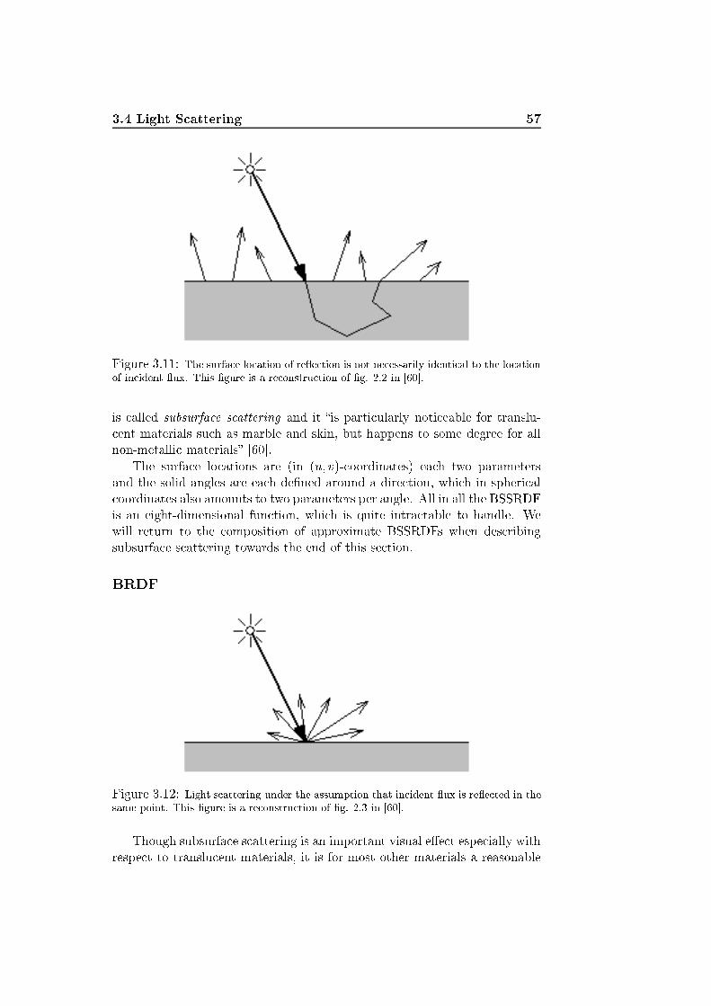
3.4 Light S attering 57

Figure 3.11: The surfa e lo ation of re�e tion is not ne essarily identi al to the lo ationof in ident �ux. This �gure is a re onstru tion of �g. 2.2 in [60℄.is alled subsurfa e s attering and it �is parti ularly noti eable for translu- ent materials su h as marble and skin, but happens to some degree for allnon-metalli materials� [60℄.The surfa e lo ations are (in (u; v)- oordinates) ea h two parametersand the solid angles are ea h de�ned around a dire tion, whi h in spheri al oordinates also amounts to two parameters per angle. All in all the BSSRDFis an eight-dimensional fun tion, whi h is quite intra table to handle. Wewill return to the omposition of approximate BSSRDFs when des ribingsubsurfa e s attering towards the end of this se tion.BRDF

Figure 3.12: Light s attering under the assumption that in ident �ux is re�e ted in thesame point. This �gure is a re onstru tion of �g. 2.3 in [60℄.Though subsurfa e s attering is an important visual e�e t espe ially withrespe t to translu ent materials, it is for most other materials a reasonable

58 The Mathemati al Model of Illuminationassumption that in ident �ux is re�e ted in the same point, see �gure 3.12.If we assume that x = x0 the surfa e is no longer s attering light internallyand we all the fa tor of proportionality a Bidire tional Re�e tan e Distri-bution Fun tion (BRDF). The BRDF is six dimensional and it is denotedfr(x;!;!0). To remove the argument x0 representing the enter of the di�er-ential area on whi h the in ident �ux impinges, we must in general integrateover the entire area of in ident �ux Ai:fr(x;!;!0) = ZAi S(x;!;x0;!0)dAi (3.21)The in ident �ux d�i of (3.20) is dependant on both the in ident dif-ferential area dAi and the in ident di�erent solid angle d!0 to whi h it is on�ned. Therefore it is not entirely omparable to d� of (3.12), rather thein ident �ux is dependant on the di�erential irradian e in ident on dAi fromd!0, meaning that d�i = d2� = dEi dAi (3.22)It then follows from (3.20) and (3.22) (still in general) that:S(x;!;x0;!0) = dLr(x;!;x0;!0)d�i = d2Lr(x;!;x0;!0)dEi dAi (3.23), fr(x;!;!0) = RAi S(x;!;x0;!0)dAi = dLr(x;!;!0)dEi (3.24)whi h shows that setting x = x0 is a simplifying assumption that avoids theintegral over Ai, and under that assumption (3.24) states that the portionof re�e ted radian e dLr at the point x within the di�erential solid angle d!is dire tly proportional to the in ident irradian e dEi on�ned within thedi�erential solid angle d!0 from the dire tion (�0; �0).To �nd a formula for dEi it follows by substitution of (3.22) in (3.13)that: 1 os �0 dEi dAid!0 dAi = Li(x;!0) ) dEid!0 = Li(x;!0) os �0 (3.25)whi h a ording to (3.24) indi ates that:fr(x;!;!0) = dLr(x;!;!0)Li(x;!0) os �0 d!0 (3.26)Suppose the unit normal n at the surfa e lo ation x is known and thatthe dire tion of the in ident solid angle is given as a normalized three-dimensional ve tor !0, then the hemispheri al-dire tional re�e ted radian e

3.4 Light S attering 59(�g. 3.10b) an be omputed using the following re ursive formula derivedfrom (3.26) by integration over the entire hemisphere:Lr(x;!) = Z fr(x;!;!0)Li(x;!0) os �0 d!0= Z fr(x;!;!0)Li(x;!0)(!0 � n) d!0 (3.27)Intuitively the BRDF (fr) spe i�es the portion of radian e in ident at asurfa e lo ation that is re�e ted in another dire tion. The BRDF at a singlepoint on a surfa e is a four-dimensional fun tion, whi h an be measured fromreal surfa es using, for example, a goniore�e tometer [126℄. Many BRDFmodels exist; both empiri al BRDFs based on sample data, physi ally basedBRDFs, and even intuitive BRDFs based on simpli ity and the quality ofresulting images. Surfa e re�e tan e is important in the spe i� ation ofdi�erent BRDFs.Re�e tan eRe�e tan e is de�ned as the ratio of re�e ted to in ident �ux:�(x) = d�rd�i (3.28)By integration over the hemisphere above x in (3.13), we an a hieve thefollowing: d�i(x)dA = Z Li(x;!0)(!0 � n) d!0 (3.29)Considering (3.27) and (3.13) we an also �nd the following equation forthe di�erential re�e ted �ux:d�r(x)dA = Z Z fr(x;!;!0)Li(x;!0)(!0 � n) d!0 (! � n) d! (3.30)Holding (3.30) and (3.29) up against ea h other reveals the followingformula for al ulation of re�e tan e:�(x) = d�rd�i = R R fr(x;!;!0)Li(x;!0)(!0 � n)(! � n) d!0 d!R Li(x;!0)(!0 � n) d!0 (3.31)To give a brief example of the usefulness of re�e tan e we an �nd theBRDF of di�use surfa es, fr;d(x), whi h by de�nition of a di�use materialis indi�erent to the dire tions of in ident and exitant light. A ording to(3.31) we �nd:

60 The Mathemati al Model of Illumination�d(x) = fr;d(x) R R Li(x;!0)(!0 � n)(! � n) d!0 d!R Li(x;!0)(!0 � n) d!0= fr;d(x)Z(! � n) d! R Li(x;!0)(!0 � n) d!0R Li(x;!0)(!0 � n) d!0= fr;d(x)�) fr;d(x) = �d(x)� (3.32)Most often it is assumed that the re�e tan e is onstant over the entiresurfa e of the di�use obje t in whi h ase the BRDF is merely a onstantgiven as fr;d = �d=�. Other more omplex BRDFs will be des ribed in later hapters of this part.BTDFWhile the BRDF, fr, spe i�es the amount of radian e that is re�e ted, we ould onsider a similar fun tion, ft, spe ifying the amount of radian e thatis refra ted. ft is alled a Bidire tional Transmittan e Distribution Fun tionBTDF and it ould be derived in a similar way only onsidering dLt insteadof dLr in (3.20).Measuring the BTDF from real surfa es is, however, harder than measur-ing the BRDF [126℄ (sin e the measurement must be done on the oppositeside of the surfa e, that is, inside the medium). In omputer graphi s per-fe tly spe ular refra tion (see se tion 3.1) is usually the only ase that is onsidered, if a more omplex distribution fun tion is needed the BTDF ismost often approximated by an empiri al model tuned by a few handpi kedparameters.Re�e tan e is a ratio that an be used in order to establish the amountof re�e ted radian e, �. If a surfa e is perfe tly spe ular no radian e will beabsorbed and the amount of refra ted radian e, that is, the transmittan e,will be 1� �.The re�e tan e of a perfe tly spe ular surfa e is a spe ial ase of (3.31).To �nd this spe ular re�e tan e without solving (3.31), we need to borrowsome theory from wave opti s. The Fresnel equations, dis overed in 1821 (seeapp. B), are based on the wave theory of light and they take polarization intoa ount. Polarization an be explained as a superposition of two transversewaves, whi h os illate in dire tions perpendi ular to ea h other and to thedire tion of propagation [30℄. The Fresnel equations �nd the amount ofre�e ted light in a medium with index of refra tion �1 in ident on a materialwith index of refra tion �2 at the angle �1 with the surfa e normal turningoutwards, refra ting light at the angle �2 with the surfa e normal turninginwards. The two omponents of polarized light are given as [60℄:

3.4 Light S attering 61�k = �2 os �1 � �1 os �2�2 os �1 + �1 os �2 (3.33)�? = �1 os �1 � �2 os �2�1 os �1 + �2 os �2 (3.34)Light usually be omes polarized due to s attering [30℄. Light emittedfrom light sour es is mostly unpolarized, or so alled natural light. Forunpolarized light the Fresnel re�e tion oe� ient, Fr, whi h is identi al tothe spe ular re�e tan e, be omes [60℄:Fr(�) = 12(�2k + �2?) = d�rd�i (3.35)Some omputationally less expensive approximations to (3.35) have beenproposed. One of them was derived by S hli k and has the following empiri alform [118℄: Fr(�) � F0 + (1� F0)(1 � os �)5 (3.36)where F0 is the value of (3.35) at normal in iden e:F0 = ��1 � �2�1 + �2�2 (3.37)BSDFUsing the Fresnel equation, the BTDF is usually in orporated in the BRDFto a ount for perfe tly spe ular refra tion. A more general model must,however, spe ify both a BRDF and a BTDF over the entire unit spheresurrounding ea h surfa e lo ation. Sin e BRDFs and BTDFs in most asesonly are de�ned on hemispheres, the more general model amounts to fourdi�erent fun tions5, whi h more onveniently an be gathered into a singlefun tion, fs, alled a Bidire tional S attering Distribution Fun tion BSDF.Parti ipating MediaIt is ommonly assumed that all media in a s ene are homogenous, and asstated previously, a ording to Hero's prin iple, light travels in straight linesin homogenous media. The result of these simplifying assumptions is thata rendering method usually an be ontent with evaluation of a distributionfun tion, su h as those des ribed above, at the visible surfa e areas of as ene.Suppose that we wish to render a loud of smoke or dust, a glass of milk,a marble statue, or human skin. In all those ases (and many others) the5Two BRDFs and two BTDFs - one of ea h for ea h side of the surfa e.

62 The Mathemati al Model of Illuminationmaterial to be rendered is inhomogenous and translu ent, meaning that thelight will refra t into the medium and s atter around before it is refra tedba k into the medium from where it ame at another surfa e lo ation. Inother words we need a di�erent rendering method for inhomogenous media.Rendering of a translu ent material will often be ombined with otherrendering te hniques that only take surfa e s attering into onsideration, thisis obvious sin e a s ene often will ontain both kinds of obje t materials. Theinhomogenous media are therefore traditionally referred to as parti ipatingmedia. The material of parti ipating media is often quite translu ent, andsin e light does not move in straight lines inside it, we must take the entirevolume of a parti ipating medium into a ount (or at least a slab lose tothe border area) when an obje t of su h material is to be rendered.Radian e is still the quantity that we want to al ulate. We must, how-ever, take into onsideration that the radiation is frequently weakened ands attered by intera tion with matter when traversing through an inhomoge-nous medium. Let �t(x) = �(x)� des ribe the extin tion oe� ient, whi his omposed of �, the mass absorption oe� ient, and �, the density of thematerial. The extin tion oe� ient �t(x) de�nes the rate of radiation thatis absorbed at lo ation x in the medium. Now, after traversing a thi knessds in the dire tion of the light's propagation, the radian e will be absorbedby the medium a ording to the extin tion oe� ient [15℄:dL(s)ds = ��(s)�L(s) = ��t(s)L(s) (3.38)All the radiation that is absorbed is not ne essarily transformed to otherkinds of energy, some or all of it may as well be s attered ba k into themedium. In order to spe ify the out-s attered radian e we must spe ify theangular distribution of the s attered radiation, this is done by means of aphase fun tion p(x;!;!0) = p(x;! �!0) whi h in the general ase must agreewith the following [15℄: Z4� p(! � !0)d!04� = $0 � 1where $0 represents the fra tion of out-s attered radian e, while 1 �$0 isthe fra tion that has been turned into other forms of energy (or radiationoutside the visible spe trum). $0 is alled the albedo for single s attering.In omputer graphi s it is most ommonly assumed that the phase fun tionis normalized to unity, that is, $0 = 1, whi h is the onservative ase ofperfe t s attering.The s attering oe� ient �s(x) is the rate of radiation that is s atteredba k into the medium at lo ation x. In the ase of perfe t s attering �s = �t.Otherwise the s attering oe� ient is given as �s = $0�t. In terms ofthi kness we an write the out-s attered radian e as:

3.4 Light S attering 63dL(s)ds = �t(s)Z4� p(s;!0)L(s;!0)d!0 (3.39)Note how (3.39) to a ertain extend resembles (3.27). For onsisten ywith other texts, and sin e it may ome in handy, we an also de�ne anabsorbtion oe� ient as �a = �t � �s = (1�$0)�t.If the medium is not a light sour e itself it is alled a s attering medium.In that ase the out-s attered radian e is the total emission from a givenpoint in the medium.Suppose the radian e transfer is pla ed in a Cartesian oordinate system(whi h is generally the ase), then the thi kness s(x;!) is dependant onboth the urrent lo ation in the medium x and the in ident dire tion !.The total hange in radian e per unit distan e for a s attering media is thengiven as:(! � r)L(x;!) = ��t(x)�L(x;!) � Z4� p(x;!;!0)L(x;!0)d!0� (3.40)Treatment of volumetri light sour es su h as �re or plasma is beyondthe s ope of this proje t, for the proper expansion of (3.40) see eg. [100℄,here we will restri t ourselves to s attering media only, and therefore (3.40)is su� ient for our purposes.In order to derive a formal solution for (3.40) it is more onvenient tokeep the notion of thi kness for a moment. The simpler form of (3.40) is thesimple addition of (3.38) and (3.39):dL(s)ds = ��t(s)�L(s)� Z4� p(s;!0)L(s;!0)d!0� (3.41)The formal solution is presented in [15℄ (though in a more general form)as:L(s) = L(0)e��(s;0) + Z s0 e��(s;s0)�t(s0)Z4� p(s0;!0)L(s0;!0)d!0ds0 (3.42)where �(s; s0) is the opti al thi kness of the material between the points sand s0, whi h is given as: �(s; s0) = Z ss0 �t(t)dtLet the s attering parti ipating medium be des ribed geometri ally by a�nite volume V � R3 , and let �V denote the boundary of V. Then rewriting(3.42) in terms of a Cartesian oordinate system results in the followingformulation of the radian e at a lo ation x in a dire tion !:

64 The Mathemati al Model of IlluminationL(x;!) = Z xx�V e��(x;x0)�t(x0)Z4� p(x;!;!0)L(x0;!0)d!0dx0+e��(x;x�V )L(x;!) (3.43)where x�V 2 �V is the losest surfa e point from x in dire tion �! ([100℄)(re all that ! is the dire tion in whi h the radian e is traveling).In omputer graphi s (3.43) is referred to as the volume rendering equa-tion, sin e �it is the equation that must be solved in order to render parti -ipating media� [60℄. In our ase it is not ompletely general sin e we have hosen to work with s attering media only, meaning that we left out theemission term. The simpler ase introdu ed at the beginning of this se tion,where we onsider the intera tion between radiation and media at the surfa eonly, of ourse, has a similar equation. This is simply alled the renderingequation and it is the subje t of se tion 3.5.The volume rendering equation is rather omplex and has only re entlybeen approa hed in real-time. Some of the most re ent real-time approxi-mations are presented in [52℄. One way to �nd a rough approximation is to onstru t a depth map of the s ene and to use this for a simple thi kness al ulation.Another approa h is to simplify the equation by pi king out a subsetof materials that have some hara teristi s in ommon. Based on those hara teristi s some simplifying assumptions an often be made. A largepart of the materials that we wish to simulate are quite dense. Materialssu h as marble, milk, leaves, and skin all have a well de�ned boundary (�V).Rendering of those relatively dense materials an be approximated usingthe original assumption that we need only onsider the surfa e area. Thisapproa h, in fa t, indi ates that we an use (3.43) to �nd an approximationof the BSSRDF (S in (3.20)).As mentioned before the visual e�e t that we wish to simulate whenusing the BSSRDF is alled subsurfa e s attering. This parti ular e�e t isespe ially visible in translu ent materials with a well-de�ned boundary, andit is treated as the on luding part of this se tion on light s attering.Subsurfa e S atteringWhy do we need to simulate subsurfa e s attering? (a) Though the e�e t isoften subtle, it gives a powerful visual ue, and (b) translu ent obje ts aremore pleasing, interesting, and realisti [52℄. Di�use materials, su h as lothand skin, often tend to be ome rough and �unfriendly� in omputer graphi swhen subsurfa e s attering is not taken into a ount.After [45℄ in whi h (3.43) is approximated using a Monte Carlo methodin ombination with a standard ray tra er, the idea mentioned, namely that

3.4 Light S attering 65the volume rendering equation an be used to de�ne an approximate BSS-RDF, has bread a series of arti les [29, 64, 105, 65, 61℄ whi h resulted in anapproximative BSSRDF model that has been used for intera tive subsurfa es attering in re ent arti les su h as [75, 46, 81, 80, 13℄.It would arry us too far to go through the theory presented in those ar-ti les. However, we an in short present some of the simplifying assumptionsthat are introdu ed and some of the results that they a hieve.First it is assumed that the phase fun tion is independent of the singles attering albedo $0, meaning that the fra tion of out-s attered radian e annot hange a ording to the phase fun tion. Instead the single s atteringalbedo is repla ed by: � = �s�tand it is assumed that the phase fun tion is normalized to unity $0 = 1.Under these assumptions �s = �t � �a 6= $0�t. Furthermore it is assumedthat the phase fun tion is a fun tion only of the phase angle, p(!;!0) = p(! �!0), meaning that the phase fun tion is the same throughout a translu entobje t. These assumptions are done to ease al ulations involving the phasefun tion.De�nition 6 (Isotropy) A medium is said to be isotropi at a point, if the radian e is independent of dire tion at thatpoint. And if the radian e is the same at all points andin all dire tions, the medium is said to be homogenous andisotropi . [15℄Next they look loser at the pro ess of subsurfa e s attering. It is ob-served that �the light distribution in highly s attering media tends to be omeisotropi . This is true even if the initial light sour e distribution and phasefun tion are highly anisotropi � [65℄. Whi h means that multiple s atteringbeneath the surfa e of a translu ent obje t an be represented by a di�usionapproximation Sd, whi h in [65℄ is given as:Sd(x;!;x0;!0) = 1�Ft(�;!)Rd(kx� x0k)Ft(�;!0) (3.44)where Ft = 1� Fr is the unpolarized Fresnel transmittan e ( f. (3.35)) andRd is the di�use re�e tan e, whi h is approximated by a dipole light sour e onsisting of two point sour es; one above the surfa e and one beneath. [75℄provides a good overview of how Rd is al ulated, while onstants measuredfor di�erent kinds of materials are provided in [65℄ whi h originally intro-du ed the dipole light sour e.

66 The Mathemati al Model of IlluminationBesides the di�usion approximation the BSSRDF given in this methodalso onsists of a single s attering term S(1)(x;!;x0;!0). The single s at-tering term de�nes how the radian e Li(x0;!0) in ident on the translu entobje t at the surfa e lo ation x0 from the dire tion !0 ontributes to the out-going radian e Lo(x;!) at the surfa e lo ation x in the dire tion ! by meansof refra tion through the translu ent obje t a ording to Fresnel terms, ab-sorption and the phase fun tion.The omplete BSSRDF model (as presented in the above mentioned seriesof arti les) is the sum of the di�usion approximation and the single s atteringterm: S(x;!;x0;!0) = Sd(x;!;x0;!0) + S(1)(x;!;x0;!0) (3.45)Most intera tive approa hes limit themselves to isotropi materials6. Inthat ase S � Sd. Lens h et al. [75℄ show how the di�use subsurfa e s at-tering re�e tan e Rd an be in orporated in a radiosity solution. Carr etal. [13℄ move this solution to the GPU. Hao et al. [46℄ in orporate Sd ina lo al illumination model, and �nally Mertens et al. [81, 80℄ use a leverhierar hi al boundary element method similar to hierar hi al radiosity withSd and report robust results. They all obtain intera tive frame rates.The intensions of this se tion (3.4) have been (a) to provide a good un-derstanding of light s attering in general, and (b) to give a brief perspe tiveon the urrent approa hes to subsurfa e s attering. We have not given allthe details, but we have provided the ne essary referen es if spe i� detailsare needed. In part III we present our own simpli�ed approa h to subsurfa es attering based on the theory of parti ipating media.This on ludes the se tion on light s attering. In the next se tion weuse the theory on light s attering to derive the rendering equation from itsoriginal enun iation.3.5 The Rendering EquationMost of the main omputer graphi s resear h areas were founded in the earlyeighties. Major global illumination te hniques su h as ray tra ing, �rst pre-sented for omputer graphi s by Turner Whitted in [137℄, and radiosity, fromGoral et al. in [40℄, were more or less based on theoreti al results from heattransfer, opti s, and radiometry. A straightforward relationship between thedi�erent te hniques was, however, not lear until Kajiya's enun iation of therendering equation in [66℄, where he shows that ray tra ing and radiositybasi ally seek to solve the same integral equation.The rendering equation is based on thermal radiation heat transfer (see[121℄) and fundamentally it derives from the same formula as has been de-6An isotropi medium orresponds to a di�use surfa e.

3.5 The Rendering Equation 67s ribed in se tions 3.2 and 3.4. In its original form the rendering equationwas given as below, [66℄:L(x;x0) = g(x;x0) ��(x;x0) + ZS �(x;x0;x00)L(x0;x00)dx00� (3.46)where x, x0, and x00 are surfa e lo ations (possibly at di�erent surfa es inthe s ene, x may be an eye point and x00 a position on a light sour e). S isthe union of all surfa es, meaning that the integral is taken over all pointsin the geometry of a s ene. g(x;x0) is a visibility term spe ifying whether ornot the point x0 is visible from x. �(x;x0) = Le(x;x0) is radian e emittedfrom the surfa e lo ation x0 rea hing the surfa e lo ation x. As des ribedin se tion 3.2 emission an result from, for example, a supply of ele tri alpower, and it should be added to the radian e re�e ted at the point x0.In order to understand the transport of light from one surfa e lo ation toanother, we must �rst prove that radian e is invariant along straight paths.Invarian e of Radian e Along Straight PathsA ording to Hero's prin iple light travels in straight lines in a homogenousmedium ( f. se tion 3.1). Therefore it is evident that light traveling througha homogenous medium from one surfa e lo ation x in a s ene towards anothery will rea h the other point provided that no o luding obje t is situatedbetween the two points.Sin e light is traveling in a straight line between two surfa e lo ations,a di�erential solid angle d!xy for radian e Lo(x;y) through a di�erentialsurfa e area dAx entered at x an be subtended by a di�erential surfa e areadAy entered at y. The subs ript o denotes that the radian e is outgoing,and the radian e leaving x and arriving at y an thus be des ribed as:Lo(x;y) = d2�o os �x d!xy dAx (3.47)Letting the subs ript i denote the radian e in ident on a surfa e, we an, onversely, de�ne the radian e arriving at y from x as:Li(y;x) = d2�i os �yd!yx dAy (3.48)Re all from se tion 3.2 that knowledge of the area subtending a solidangle gives us a possibility to determine the solid angle by proje tion of thearea on a sphere entered at the point where the solid angle is formed.Consider the solid angle ! formed at x subtended by a surfa e area Ay entered around y, �gure 3.13 pi tures the di�erential ase. Let r be thedistan e between x and y, then a ording to (3.7) ! = As=r2, where As isthe area of Ay proje ted to the sphere s of radius r entered at x. If Ay is

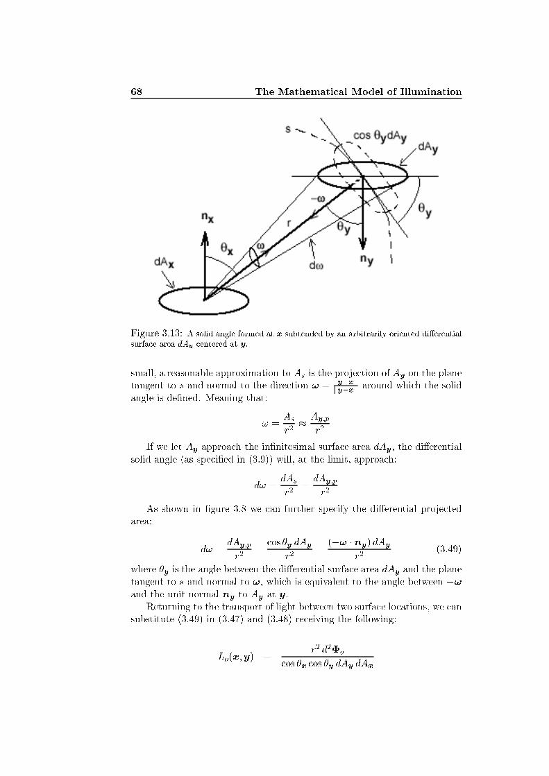
68 The Mathemati al Model of Illumination

Figure 3.13: A solid angle formed at x subtended by an arbitrarily oriented di�erentialsurfa e area dAy entered at y.small, a reasonable approximation to As is the proje tion of Ay on the planetangent to s and normal to the dire tion ! = y�xky�xk around whi h the solidangle is de�ned. Meaning that:! = Asr2 � Ay;pr2If we let Ay approa h the in�nitesimal surfa e area dAy, the di�erentialsolid angle (as spe i�ed in (3.9)) will, at the limit, approa h:d! = dAsr2 = dAy;pr2As shown in �gure 3.8 we an further spe ify the di�erential proje tedarea: d! = dAy;pr2 = os �y dAyr2 = (�! � ny) dAyr2 (3.49)where �y is the angle between the di�erential surfa e area dAy and the planetangent to s and normal to !, whi h is equivalent to the angle between �!and the unit normal ny to Ay at y.Returning to the transport of light between two surfa e lo ations, we ansubstitute (3.49) in (3.47) and (3.48) re eiving the following:Lo(x;y) = r2 d2�o os �x os �y dAy dAx

3.5 The Rendering Equation 69Li(y;x) = r2 d2�i os �y os �x dAx dAyA ording to the �rst law of thermodynami s (whi h is also known as thelaw of onservation of energy, see eg. [11℄) the total energy of a system andits surroundings is onstant. Meaning that all the energy outgoing at x thatwill rea h y (whi h by Hero's prin iple will be all light that is not o luded)without being absorbed by parti ipating media, will also be in ident at y.If light is o luded Lo(x;y) = Li(y;x) = 0. Therefore it is indeed the asethat in a va uum: Lo(x;y) = Li(y;x) (3.50)�Returning to the original problem; we seek to simulate human visionin a digital s ene and show the result on a monitor. Basi ally this meansthat we want to �nd the total radian e in ident at the di�erential surfa earea representing the eye. The total radian e in ident at the eye enteredaround x is either radian e Li(x;x0) transported from all surfa e lo ationsin the s ene to the eye, or the radian e Li(x;!) in ident at the eye from alldire tions given by the hemisphere over the eye.The rendering equation des ribes the problem in terms of surfa e lo a-tions only, while the original de�nition of radian e des ribes the problem interms of one surfa e lo ation and dire tional solid angles on the hemisphereabove it.To show onsisten y between the rendering equation and the theory ofradian e and light s attering that has been presented previously in this hap-ter, we will in the remainder of this se tion show why the rendering equationis an alternative formulation of the hemispheri al problem that was presentedwith respe t to re�e tion in se tion 3.4.The invarian e of radian e along straight lines gives a ue about why itis sometimes onvenient to onsider the radian e in terms of surfa e lo a-tions and an integral over all surfa e areas rather than an integral over thehemisphere as presented in (3.27).L(x;x0) is referred to as transport radian e and mathemati ally we ande�ne it as: d3Qdt dx dx0 = d2�dx dx0 = L(x;x0) (3.51)Combining (3.51) with (3.13) we will a ording to (3.49) retrieve thefollowing onne tion between transport radian e and dire tional radian e:L(x;!) = 1 os � d2�d! dx = r2 os � os �0 d2�dx dx0 = r2 os � os �0L(x;x0) (3.52)

70 The Mathemati al Model of IlluminationSuppose we are onsidering the outgoing radian e from the di�erentialsurfa e area entered around x0. Inserting the results from (3.49) and (3.52)in (3.46) we retrieve the following version of the rendering equation:Li(x;�!) os � os �0r2 = g(x;x0)�Le(x0;!) os � os �0r2+Z �(x;x0;x00)Li(x0;!0) os �0 os �00r2 r2 os �00d!0�) Li(x;�!) = g(x;x0)�Le(x0;!) + Z fr(x0;!;!0)Li(x0;!0) os �0 d!0�where fr(x;!;!0) os � os �0=r2 = �(x;x0;x00).Now, if we wish to �nd the exitant (or outgoing) radian e at lo ation x0rather than the radian e in ident at lo ation x, all radian e will be al ulatedin the same point and in that ase we need not worry about the visibilityterm (g(x;x) = 1). Then it follows that:Lo(x0;!) = Le(x0;!) + Z fr(x0;!;!0)Li(x0;!0)(n � !0) d!0= Le(x0;!) + Lr(x0;!) (3.53)where it should be noted that Lr is exa tly the same as the re�e ted radian edes ribed in (3.27).Comparing transport radian e and dire tional radian e, we know fromradiometry that dire tional radian e most losely resembles what the eyeper eive as olor, the hemispheri al formulation of the rendering equation(3.53) is therefore better to use than Kajiya's original formulation (3.46).Still it might be useful to al ulate the re�e ted radian e by integration oversurfa e areas rather than the hemisphere. Therefore the rendering equa-tion has an area formulation as well. The area formulation is derived bysubstitution of (3.49) in the integral representing the re�e ted radian e:Lo(x;!) = Le(x;!)+ZA fr(x;!;!0)Li(x;!0)g(x;y)(nx � !0)(ny � �!0)r2xy dAyFor onsisten y with other texts (eg. [30℄) we will rename the visibilityfun tion to V (x;y) = g(x;y) and de�ne a geometry term G(x;y):G(x;y) = (nx � !0)(ny � �!0)r2xyThe resulting area formulation of the rendering equation is then:

3.6 Light Transport 71Lo(x;!) = Le(x;!) + ZA fr(x;!;!0)Li(x;!0)V (x;y)G(x;y) dAy (3.54)Having des ribed the rendering equation all there is left to do is to solve it.Consider, however, the re ursive nature of the re�e ted radian e term, thismakes the rendering equation impossible to solve analyti ally. The followingse tion on light transport theory will investigate the re ursive re�e tion termand introdu e a few integral operators for ease of notation.3.6 Light TransportDuring this hapter we have des ribed a mathemati al model through whi hthe illumination of an environment an be simulated. Radian e is the quan-tity that we are interested in and the rendering equation states how radian eis al ulated at an arbitrary lo ation in an arbitrary dire tion.Evaluation of the rendering equation is, however, not straight forward.In the remainder of this se tion we shall take a loser look. Suppose weare looking at a surfa e lo ation x. A ording to the invarian e of radian ealong straight paths (3.50) the radian e rea hing the eye, that is, the olorwe see, is equivalent to the exitant radian e at x in the dire tion towards theeye. This quantity is exa tly what the rendering equation (3.53) �nds. Theemission term Le is only non-zero if the obje t is a light sour e. Cal ulationof Le is des ribed in se tion 3.2. The re�e ted radian e term Lr �nds thehemispheri al-dire tional ontribution (see �gure 3.10b), whi h is the sum ofall radian e in ident over the hemisphere. Now, a ording to the invarian eof radian e along straight paths, ea h radian e in ident from the dire tion!0 on the hemisphere is equivalent to the exitant radian e at the �rst pointinterse ted if we tra e a ray ba kwards in the dire tion !0. This exitantradian e is again found by evaluation of the rendering equation and so on andso forth. The re ursion be omes apparent, sin e Li(x;!0) in the renderingequation is substituted by Lo(y;�!0), whi h is again substituted by therendering equation evaluated at y in the dire tion �!0.To handle the rendering equation more on isely, we an introdu e a fewlinear integral operators7. Operator notation is a onvenient way to des ribelight transport. We an de�ne a s attering operator S ([17℄), whi h representsthe integral in (3.27) �nding re�e ted radian e from in ident radian e. Stransforms a ertain (in ident) radian e distribution, Li, over all points anddire tions to another distribution, Lr, that gives the re�e ted radian e valuesafter one re�e tion [30℄. This means that S depends on all the di�erentBRDFs de�ned for di�erent materials in a s ene.7Integral operators are a spe ial ase of the transformers introdu ed in array theory( f. se . 2.1).

72 The Mathemati al Model of IlluminationHaving the s attering operator S at our disposal we an rewrite the hemi-spheri al version of the rendering equation using the fun tional approa hdes ribed in se tion 2.1, whi h results in the following on ise form:Lo = Le + SLi (3.55)The result of S applied to a radian e distribution Li over all pointsand dire tions (A � ) is e�e tively a hemispheri al-dire tional re�e tan edistribution fun tion (HDRDF) applied to all points and dire tions.Be ause of (3.50) another operator alled the propagation operator P,transforming an exitant radian e distribution to an in ident radian e distri-bution, an be de�ned. In light of the propagation operator the renderingequation an be written as: Lo = Le + SPLo (3.56)where it shows immediately that the rendering equation is re ursive.For onvenien e we de�ne a new operator representing the ompositionof s attering and propagation To = SP alled the exitant transport operator.We an now expand the rendering equation as a Neumann series:Lo = Le + ToLo= Le + To(Le + ToLo)= Le + To(Le + To(Le + ToLo))= Le + ToLe + T 2o Le + T 3o Lo= 1Xn=0T no Le (3.57)where the supers ript n denotes that the outgoing radian e has been s at-tered n times. The path of light through a s ene expressed by the propaga-tion, s attering, and transport operators is illustrated in �gure 3.14.The physi al interpretation of (3.57) is that we an split the renderingequation up into omponents of radian e that has s attered on e, twi e,thri e, et . [66℄ (ea h s attering is often referred to as a light boun e). Thisobservation is the most important point in this se tion. It indi ates that we an des ribe the illumination of a s ene by means of the light's path throughthe s ene from the light sour e to the eye point.Light Transport NotationWhen light intera ts with matter the resulting s attering is highly dependanton the material properties. Sin e we know that the rendering equation is thesum of ontributions from di�erent light paths ( f. (3.57)), lassi� ation of

3.6 Light Transport 73

Figure 3.14: A simple illustration of light transport. From top left to bottom right:Le, P Le, SPLe or ToLe, PT oLe, ToToLe or T 2o Le, and PT 2oLe. The sequen e ould be ontinued inde�nitely.light paths a ording to the materials they have intera ted with along theway would indeed be useful. Paul S. He kbert [48℄ introdu ed a notation,now alled the light transport notation, where:� L is a light sour e� E is the eye (or the virtual amera)� S is a spe ular surfa e� D is a di�use surfa eJuxtaposition of these symbols de�nes a light path, for example, LDEdenotes radian e from a light sour e re�e ted di�usely on e before rea hingthe eye, and LDSE is a di�use surfa e lit by a light sour e and seen by re�e tionon a spe ular surfa e (su h as a mirror).A lass of light paths is de�ned using the following symbols in ombina-tion with the letters given above [60, p. 31℄:� (k)+ one or more k events� (k)* zero or more k events� (k)? zero or one k event� (kjk') a k or a k' eventmeaning that L(SjD)*E is a lass in whi h all light paths �t.The advantage of light transport notation is that some visual e�e ts areoften due to a ertain lass of light paths. If a method for the simulation ofone spe i� visual e�e t is found, we an split L(SjD)*E into sub lasses for

74 The Mathemati al Model of Illuminationdi�erent visual e�e ts and use di�erent methods for their solutions. Onlywe must make sure never to add the same light path into the integral morethan on e. An example is a method for mirror e�e ts. Mirrors are simulatedby the light paths given as L(SjD)*SE. If a spe i� method is used for mirrore�e ts other rendering methods used for the same s ene are only allowedto add light paths of the lass L(SjD)*DE to the integral of the renderingequation.Light transport notation also gives a on ise way to des ribe whi h partof the rendering equation that a spe i� rendering method an solve. Classi ray tra ing, for example, only solves the paths given as LD?S*E, while lassi radiosity solves the paths LD*E only. Ray tra ing and radiosity are des ribedin hapter 4.Re ipro ity of the BRDFA ording to Ni odemus et al. [88, p. 40℄ (and many later sour es) itis a fundamental property of the BRDF that, �by Helmholtz re ipro ity,whi h holds in the absen e of polarization and magneti �elds�, the BRDFis independent of the dire tion in whi h light �ows. That is, we may swapthe in ident and exitant dire tions and the BRDF remains un hanged:fr(x;!;!0) = fr(x;!0;!) (3.58)This property of the BRDF is quite important sin e it allows us to solvethe rendering equation by tra ing the radian e ba kwards through the s ene.The propagation and s attering is, a ording to the invarian e along straightpaths and the re ipro ity respe tively, the same as that of �gure 3.14 only,when tra ing the radian e ba kwards, we start at the eye point instead of thelight sour e. This gives rise to a dual understanding of the light transportproblem whi h is brie�y introdu ed in the remainder of this se tion.Importan eIf we tra e radian e ba kwards through the s ene, we annot know the exa tvalue of the radian e in the same way as we an al ulate the initial emissionterm before tra ing radian e from the light sour e. Instead we know thatthe radian e rea hing the eye is 100% of interest to us. In [99℄ Pattanaikand Mudur introdu ed the term importan e W , whi h has been given severalde�nitions in the literature, it is, however, ommonly de�ned as �the fra tionof radian e that ontributes (dire tly or indire tly) to the region of interest�[17, p. 4℄, and we shall use it as su h. Meaning that the radian e rea hingthe eye has the importan e We(xeye;!) = 1.Importan e has the exa t same properties as radian e, only it propagatesin the opposite dire tion and solves the dire tional dual problem. Importan ealso has an exitant (Wo) and an in ident (Wi) representation, and a ording

3.6 Light Transport 75to the invarian e of radian e along straight paths it is given, if x and y aremutually visible, that: Wi(x;!) =Wo(y;�!) (3.59)Suppose we de�ne a set S � A�, where A denotes all the surfa e pointsin a s ene and denotes the hemisphere, su h that ea h element (x;!eye) 2S is a point x seen dire tly from the eye. !eye is the dire tion towards theeye at the point x. Then a ording to (3.59) Lo(S) fully ontributes to theregion of interest, and we an write:We(x;!) = � 1 if (x;!) 2 S0 if (x;!) =2 S (3.60)Then, in light of (3.58), (3.59), and (3.60), we an de�ne an equationfor al ulation of in ident importan e, whi h is quite similar to the render-ing equation. This equation is alled the response fun tion (or potentialfun tion):Wi(x;!) =We(x;!) + Zx fr(x;!;!0)Wo(x;!0) os �0d!0 (3.61)where n is the surfa e normal at x, and x denotes all the dire tions overthe hemisphere from where radian e was in ident at the point x.In exa tly the same way as we did previously with the rendering equation,we an introdu e an in ident transport operator Ti = PS and write (3.61) inthe following way: Wi =We + TiWi (3.62)Though we will not go into the theory of adjoint operators, we will brie�ymention that if we let O� denote the adjoint of O, then Ti = PS = P�S� =(SP)� = T �o , whi h shows that the in ident transport operator is the adjointof the exitant transport operator. For more information on adjoint operatorsin rendering we refer to [17℄ and [30℄.Importan e is interesting sin e it gives us the opportunity to start arendering algorithm both at the light sour e and at the eye point, and to letimportan e and radian e meet midway. We shall exploit this notion in therendering method that we develop in part III.This on ludes the theory that we wish to present on light transport. Inthe following se tion we shall brie�y des ribe the lo al and global illumina-tion models in terms of the theory that has been presented in this hapter.

76 The Mathemati al Model of Illumination3.7 Lo al vs. Global IlluminationAs des ribed introdu torily in hapter 1 a lo al illumination model treatsea h point in a s ene as an isolated ase where exitant radian e is dependanton the lo ations of light sour es and on the lo ation of the eye only. In termsof the rendering equation:Llo al(x;!eye) = Le(x;!eye) + n�1Xi=0 fr(x;!eye;!0i)Le(yi; !0i)(n � !0i)where n is the number of light sour es, yi is the position of the i'th lightsour e, !0i is the dire tion towards the i'th light sour e, and n is as alwaysthe surfa e normal at the lo ation x.The assumption that ea h point is independent of the surrounding ge-ometry results in some serious short- omings of lo al illumination.In terms of light transport lo al illumination handles the light pathsL(SjD)?E only. Also note that lo al illumination approximate light sour esas single points in spa e. To get a more orre t result the light sour esought to be modeled as surfa e areas, and then the area formulation of therendering equation should have been used instead. The result is that thevisibility term has been left out in lo al illumination, whi h has the e�e tthat s enes lit with a lo al illumination model do not feature shadows.Lo al illumination models are useful for simple shading only. Their ad-vantage is that they are omputationally very inexpensive. Until re entlylo al illumination supplemented by an approximative shadow algorithm wasthe de fa to standard in most appli ations featuring real-time rendering.Global illumination is the term used for models that approximate therendering equation more losely than lo al illumination does. The renderingmethods for full global illumination simulates all lasses of light paths exa tlyon e: L(SjD)*E. Most global illumination methods, however, only simulatea subset of those light paths.As mentioned before lassi ray tra ing simulates the paths LD?S*E, while lassi radiosity simulates LD*E. Later approa hes expand these te hniquesor ombines them, in the latter ase they are alled hybrid methods.A hybrid method for simulation of full global illumination was exa tlywhat led He kbert to his very useful light transport notation, see [48℄. He k-bert's method has a light pass shooting photons into the s ene and depositingthe photon's power in a radiosity texture, this models the paths LS*D. Be-sides he has an eye pass tra ing importan e in order to model the paths DS*E.Now, progressive re�nement of the radiosity textures, that is, progressive re-emission of photons from the brightest surfa e, will repeat the paths (S*D)an arbitrary number of times. Combination of the progressively re�ned lightpass and the eye pass will thereby a ount for all light paths: L(S*D)*S*E= L(SjD)*E [48℄.

3.8 Solving Re ursive Integrals 77Methods su h as He kbert's �adaptive radiosity textures� are also referredto as multi-pass methods. In fa t, He kbert's method losely resembles thewidely used multi-pass method alled photon mapping, whi h was developedby Henrik Wann Jensen in [53, 63, 54, 62, 57, 55, 56, 58, 59, 60℄. There areimportant di�eren es, however, and photon mapping will be des ribed inmore detail in hapter 4.The next se tion will take a super� ial look at some of the numeri almethods that an be employed in order to solve the problem of in�nitere ursions, whi h is inherent in global illumination.3.8 Solving Re ursive IntegralsA Fredholm integral equation of the se ond kind is of the following form [98℄:y(x) = f(x) + �Z ba K(x; t)y(t)dtIf we ompare this form with (3.53) or (3.54), it is obvious that therendering equation is indeed a Fredholm equation of the se ond kind, andas su h it annot be solved analyti ally, ex ept for trivial ases. The optionwe have left is to use numeri al algorithms for the solution of the renderingequation. There are two basi approa hes: �nite element and point sampling(or Monte Carlo) te hniques, all others are derived from them [124℄.The basi idea of �nite element te hniques is to establish a system oflinear equations, whi h has a solution approximating the original integral.More te hni ally the exa t solution of the Fredholm equation lives in anin�nite-dimensional spa e. If we proje t the fun tion (y in the formula-tion above, Lo in the rendering equation) into a �nite-dimensional subspa espanned by some orthogonal basis fun tions, then an approximative solutionfor the equation an be derived, see [124℄ for further details.Radiosity [40, 18, 94℄ is based on the �nite element approa h. The ra-diosity method (named after the radiometri quantity radiosity, B, whi his equivalent to the exitant radian e, M) takes advantage of the fa t thatre�e ted radian e and radiosity are usually pie ewise smooth fun tions overa surfa e. If this is the ase, they an be approximated by smooth �nite-dimensional fun tions. The problem is that only di�use materials have theseproperties and therefore the fundamental assumption in radiosity is that allmaterials in a s ene are perfe tly di�use. This indu es serious limitationsto the radiosity approa h. The advantage, on the other hand, is that theresulting illumination looks smooth and pleasing.Monte Carlo methods basi ally approximate the integrand by taking alarge number of point samples distributed a ording to a probability den-sity fun tion (PDF). The phenomenon average8 is the average of the sample8A long-term average of data from an underlying random phenomenon, see [104℄

78 The Mathemati al Model of Illuminationpoints found a ording to the PDF. Due to the Law of Large Numbers theprobability that the phenomenon average is equal to the exa t value of theintegral onverges to unity as the number of samples in reases towards in-�nity, see [30℄ or [124℄ for further details.Distribution ray tra ing9 [20, 133℄ is based on Monte Carlo te hniques.The simple form of distribution ray tra ing uses a osine lobe for samplingover the hemisphere, and reje tion sampling if re�e tion is on�ned to a ertain solid angle by the BRDF at the urrent surfa e point. Though Cooket al. [20℄ in 1984 only had a verbal presentation of the rendering equation10,their algorithm in ludes how the following should be done at ea h positionseen from the eye point:� Sampling of the light sour es for shadow al ulations.� Sampling around the mirror dire tion for re�e tions.� Sampling around the dire tion of transmitted light for refra tions.The algorithm stops at a single level of distributed re�e tions and re-fra tions to avoid the ombinatorial explosion, meaning that it models thelight paths L(SjD)?(SjD)?E. Ward et al. [133℄ presents an idea alled irradi-an e ashing, whi h introdu es the assumption of smooth indire t illumina-tion in order to make multiple di�use interre�e tions more omputationallytra table in distribution ray tra ing.Monte Carlo methods are on eptually simpler than �nite element meth-ods, but the large amount of samples needed often results in very slow on-vergen e. Most often the sample points will be too few and varian e will bevisible as high-frequen y noise in the image. Unfortunately the eye is moreeasily distra ted by high-frequen y noise [60℄ as ompared to the smoothedimages rendered using �nite element methods. On the other hand, the sys-temati errors that an o ur in �nite element methods (be ause of the re-du tion of dimensions in the integral), will not o ur in images renderedusing Monte Carlo te hniques.In this se tion we have given a short introdu tion to the two basi nu-meri al algorithms that an be employed in order to solve re ursive integralequations. Besides we have given two examples to illustrate how these al-gorithms are appli able to the problem of solving the rendering equation.Knowledge of the two basi numeri al te hniques, supported by the rest ofthe theory des ribed in this hapter, should, hopefully, make it easier to las-sify and understand the di�erent rendering te hniques that we will presentthroughout the remainder of this part.9Distribution ray tra ing was �rst alled distributed ray tra ing. In [48℄ He kbertargued that the term distributed ray tra ing was onfusing be ause of the parallel hardware onnotations of ray tra ing. Therefore the term was hanged.10Re all that the rendering equation was not known in the area of omputer graphi suntil Kajiya introdu ed it in 1986 in [66℄.

Chapter 4Traditional Approa hes toRealisti Image Synthesis

All art is but imitation of nature.Lu ius Annaeus Sene a (4 BC. - 65 AD.)

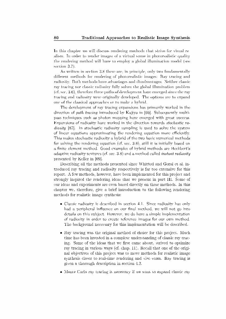
80 Traditional Approa hes to Realisti Image SynthesisIn this hapter we will dis uss rendering methods that strive for visual re-alism. In order to render images of a virtual s ene in photorealisti qualitythe rendering method will have to employ a global illumination model (seese tion 3.7).As written in se tion 3.8 there are, in prin iple, only two fundamentallydi�erent methods for rendering of photorealisti images: Ray tra ing andradiosity. Both methods have advantages and disadvantages. Neither lassi ray tra ing nor lassi radiosity fully solves the global illumination problem( f. se . 3.6), therefore three paths of development have emerged sin e the raytra ing and radiosity were originally developed. The options are to expandone of the lassi al approa hes or to make a hybrid.The development of ray tra ing expansions has primarily worked in thedire tion of path tra ing introdu ed by Kajiya in [66℄. Subsequently multi-pass te hniques su h as photon mapping have emerged with great su ess.Expansions of radiosity have worked in the dire tion towards sto hasti ra-diosity [87℄. In sto hasti radiosity sampling is used to solve the systemof linear equations approximating the rendering equation more e� iently.This makes sto hasti radiosity a hybrid of the two basi numeri al methodsfor solving the rendering equation ( f. se . 3.8), still it is initially based ona �nite element method. Good examples of hybrid methods are He kbert'sadaptive radiosity textures ( f. se . 3.8) and a method alled instant radiositypresented by Keller in [69℄.Des ribing all the methods presented sin e Whitted and Goral et al. in-trodu ed ray tra ing and radiosity respe tively is far too extensive for thisreport. A few methods, however, have been implemented for this proje t andstrongly inspired the rendering ideas that we present in part III. Some ofour ideas and experiments are even based dire tly on these methods. In this hapter we, therefore, give a brief introdu tion to the following renderingmethods for realisti image synthesis:� Classi radiosity is des ribed in se tion 4.1. Sin e radiosity has onlyhad a peripheral in�uen e on our �nal method, we will not go intodetails on this subje t. However, we do have a simple implementationof radiosity in order to reate referen e images for our own method.The ba kground ne essary for this implementation will be des ribed.� Ray tra ing was the original method of hoi e for this proje t. Mu htime has been invested in a omplete understanding of lassi ray tra -ing. Some of the ideas that we �rst ame about, strived to optimizeray tra ing in various ways ( f. hap. 11). Re all that one of the origi-nal obje tives of this proje t was to move methods for realisti imagesynthesis loser to real-time rendering and vise versa. Ray tra ing isgiven a thorough des ription in se tion 4.2.� Monte Carlo ray tra ing is ne essary if we want to expand lassi ray

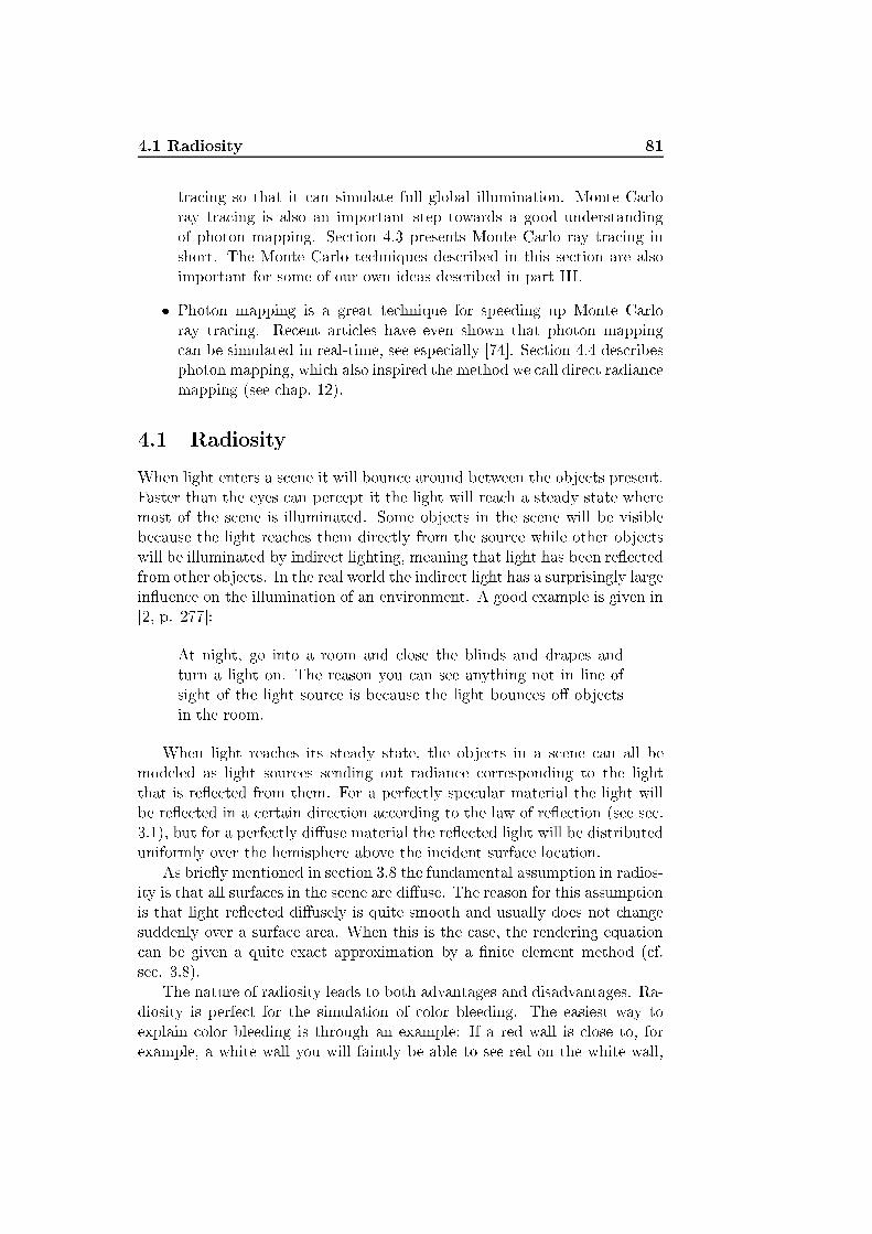
4.1 Radiosity 81tra ing so that it an simulate full global illumination. Monte Carloray tra ing is also an important step towards a good understandingof photon mapping. Se tion 4.3 presents Monte Carlo ray tra ing inshort. The Monte Carlo te hniques des ribed in this se tion are alsoimportant for some of our own ideas des ribed in part III.� Photon mapping is a great te hnique for speeding up Monte Carloray tra ing. Re ent arti les have even shown that photon mapping an be simulated in real-time, see espe ially [74℄. Se tion 4.4 des ribesphoton mapping, whi h also inspired the method we all dire t radian emapping (see hap. 12).4.1 RadiosityWhen light enters a s ene it will boun e around between the obje ts present.Faster than the eyes an per ept it the light will rea h a steady state wheremost of the s ene is illuminated. Some obje ts in the s ene will be visiblebe ause the light rea hes them dire tly from the sour e while other obje tswill be illuminated by indire t lighting, meaning that light has been re�e tedfrom other obje ts. In the real world the indire t light has a surprisingly largein�uen e on the illumination of an environment. A good example is given in[2, p. 277℄:At night, go into a room and lose the blinds and drapes andturn a light on. The reason you an see anything not in line ofsight of the light sour e is be ause the light boun es o� obje tsin the room.When light rea hes its steady state, the obje ts in a s ene an all bemodeled as light sour es sending out radian e orresponding to the lightthat is re�e ted from them. For a perfe tly spe ular material the light willbe re�e ted in a ertain dire tion a ording to the law of re�e tion (see se .3.1), but for a perfe tly di�use material the re�e ted light will be distributeduniformly over the hemisphere above the in ident surfa e lo ation.As brie�y mentioned in se tion 3.8 the fundamental assumption in radios-ity is that all surfa es in the s ene are di�use. The reason for this assumptionis that light re�e ted di�usely is quite smooth and usually does not hangesuddenly over a surfa e area. When this is the ase, the rendering equation an be given a quite exa t approximation by a �nite element method ( f.se . 3.8).The nature of radiosity leads to both advantages and disadvantages. Ra-diosity is perfe t for the simulation of olor bleeding. The easiest way toexplain olor bleeding is through an example: If a red wall is lose to, forexample, a white wall you will faintly be able to see red on the white wall,

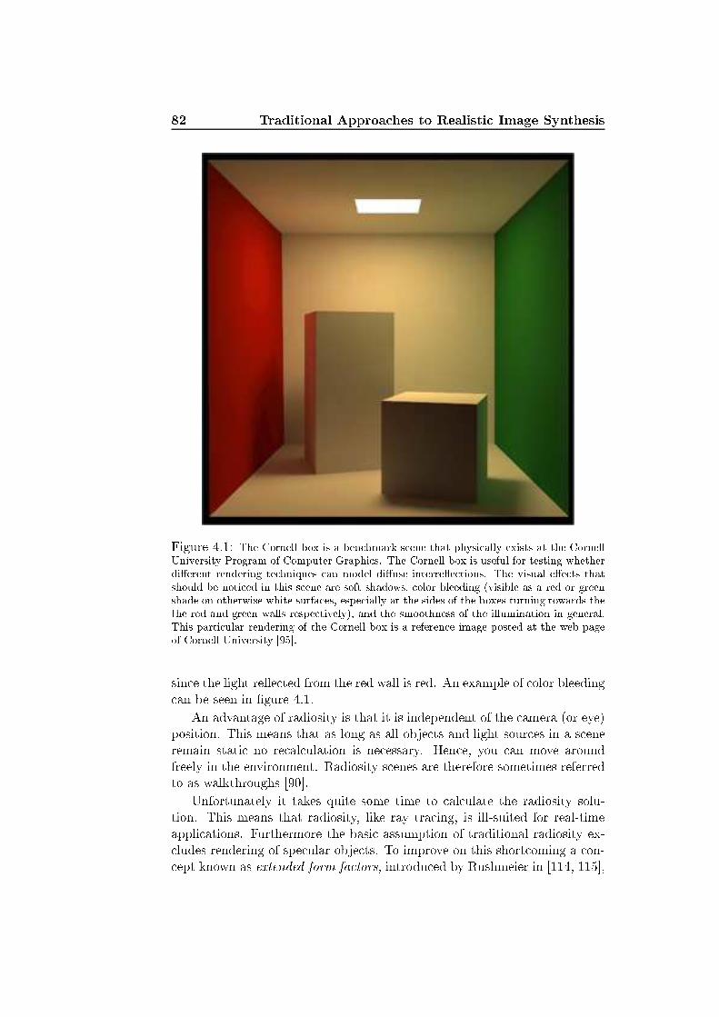
82 Traditional Approa hes to Realisti Image Synthesis

Figure 4.1: The Cornell box is a ben hmark s ene that physi ally exists at the CornellUniversity Program of Computer Graphi s. The Cornell box is useful for testing whetherdi�erent rendering te hniques an model di�use interre�e tions. The visual e�e ts thatshould be noti ed in this s ene are soft shadows, olor bleeding (visible as a red or greenshade on otherwise white surfa es, espe ially at the sides of the boxes turning towards thethe red and green walls respe tively), and the smoothness of the illumination in general.This parti ular rendering of the Cornell box is a referen e image posted at the web pageof Cornell University [95℄.sin e the light re�e ted from the red wall is red. An example of olor bleeding an be seen in �gure 4.1.An advantage of radiosity is that it is independent of the amera (or eye)position. This means that as long as all obje ts and light sour es in a s eneremain stati no re al ulation is ne essary. Hen e, you an move aroundfreely in the environment. Radiosity s enes are therefore sometimes referredto as walkthroughs [90℄.Unfortunately it takes quite some time to al ulate the radiosity solu-tion. This means that radiosity, like ray tra ing, is ill-suited for real-timeappli ations. Furthermore the basi assumption of traditional radiosity ex- ludes rendering of spe ular obje ts. To improve on this short oming a on- ept known as extended form fa tors, introdu ed by Rushmeier in [114, 115℄,

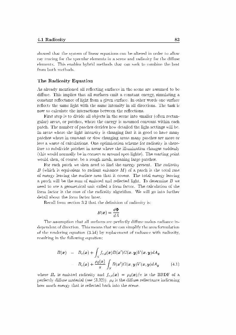
4.1 Radiosity 83showed that the system of linear equations an be altered in order to allowray tra ing for the spe ular elements in a s ene and radiosity for the di�useelements. This enables hybrid methods that an seek to ombine the bestfrom both methods.The Radiosity EquationAs already mentioned all re�e ting surfa es in the s ene are assumed to bedi�use. This implies that all surfa es emit a onstant energy, simulating a onstant re�e tan e of light from a given surfa e. In other words one surfa ere�e ts the same light with the same intensity in all dire tions. The task isnow to al ulate the intera tions between the re�e tions.First step is to divide all obje ts in the s ene into smaller (often re tan-gular) areas, or pat hes, where the energy is assumed onstant within ea hpat h. The number of pat hes de ides how detailed the light settings will be.In areas where the light intensity is hanging fast it is good to have manypat hes where in onstant or slow hanging areas many pat hes are more orless a waste of al ulations. One optimization s heme for radiosity is there-fore to subdivide pat hes in areas where the illumination hanges suddenly(this would normally be in orners or around spot lights). The starting pointwould then, of ourse, be a rough mesh, meaning large pat hes.For ea h pat h we then need to �nd the energy present. The radiosityB (whi h is equivalent to radiant exitan e M) of a pat h is the total rateof energy leaving the surfa e area that it overs. The total energy leavinga pat h will be the sum of emitted and re�e ted light. To determine B weneed to use a geometri al unit alled a form fa tor. The al ulation of theform fa tor is the ore of the radiosity algorithm. We will go into furtherdetail about the form fa tor later.Re all from se tion 3.2 that the de�nition of radiosity is:B(x) = d�dAThe assumption that all surfa es are perfe tly di�use makes radian e in-dependent of dire tion. This means that we an simplify the area formulationof the rendering equation (3.54) by repla ement of radian e with radiosity,resulting in the following equation:B(x) = Be(x) + ZS fr;d(x)B(x0)G(x;y)V (x;y)dAy= Be(x) + �d(x)� ZS B(x0)G(x;y)V (x;y)dAy (4.1)where Be is emitted radiosity and fr;d(x) = �d(x)=� is the BRDF of aperfe tly di�use material (see (3.32)). �d is the di�use re�e tan e indi atinghow mu h energy that is re�e ted ba k into the s ene.

84 Traditional Approa hes to Realisti Image SynthesisIn order to solve (4.1) using a �nite element method it is assumed thatradiosity is onstant over ea h pat h. In that ase the radiosity of one pat h an be used as a basis element for a system of linear equations. The trueradiosity is, in fa t, only rarely pie ewise onstant, but due to linear inter-polation a ross ea h pat h the di�eren e between the approximation B0 andthe true version B is, in pra tise, rarely visible.The inter hange of energy between two pat hes Pi and Pj is a fun tionof the geometri al relationships between them. This in ludes for examplethe distan e between them and their relative orientation. The more paralleland the loser to ea h other the two pat hes are, the higher will the energyex hange between them be.We an �nd the radiosity of a pat h Pi due to all other pat hes in thes ene, Pj ; j = 1; : : : ; n, where n is the number of pat hes in the s ene, as[30℄: B0i = Be;i + �i nXj=1 FijB0j (4.2)where B0k (due to the assumption of onstant radiosity over ea h pat h) isthe average radiosity of pat h k, �i is the di�use re�e tan e of pat h i, Be;i isemitted radiosity of the pat h i, and Fij are the pat h-to-pat h form fa tors,given as [60℄: Fij = 1Ai ZSi ZSj G(x;y)V (x;y)� dAjdAi (4.3)The form fa tors represent the fra tion of energy leaving pat h j andarriving at pat h i. Si is the set of points in pat h i and Sj is the set ofpoints in pat h j. The following three properties of form fa tors are derivedin [30, p. 150℄:1. The form fa tors are zero or positive in a s ene onsisting of losedopaque obje ts.2. If the s ene is losed: nXj=1 Fij = 1If the s ene is not losed: nXj=1 Fij < 13. The form fa tors satisfy the following re ipro ity relation:AiFij = AjFji

4.1 Radiosity 85Being the most omplex element in the radiosity equation (4.1), the al- ulation of form fa tors usually determines the rendering time when usingradiosity. If we exploit the re ipro ity relation given above (property 3) thereis an opportunity to halve the number of form fa tors that we must ompute.The simplest way to al ulate an approximated form fa tor is to assumethat the energy transfer between two pat hes is onstant no matter whi hpoint x we hoose on the pat h i, and whi h point y we hoose on the pat hj. In that ase al ulation of the pat h-to-pat h form fa tor simpli�es to:Fij � 1Ai G(x;y)V (x;y)� AjAi = G(x;y)V (x;y)� Aj (4.4)where the enter of pat h i is hosen as x and the enter of pat h j is hosenas y.This is one of the approa hes that is in luded in our simple radiosity im-plementation. Another approa h al ulates form fa tors using the hemi ubemethod, whi h is des ribed in the following.The Hemi ube methodThe hemi ube method is presented in [18℄ and shortly reprodu ed here. Inorder to al ulate the form fa tor Fij between two pat hes Pi and Pj animaginary ube is onstru ted around the enter of the re eiving pat h (Pi).The upper half of the surfa e of the ube is alled the hemi ube. The fa esof the hemi ube are divided into square pixels at a given resolution. Theidea is then to proje t the pat h Pj onto the �ve planar surfa es, see �gure4.2.Re all, however, that the energy re eived at the pat h Pi is dependent onthe lo ation and orientation of the pat h Pj . Therefore the ontribution ofea h square pixel to the form fa tor is also dependent on the pixel lo ationand orientation. For ea h pixel pq we an therefore de�ne a delta form fa tor�Fq, and the sum of all the delta form fa tors will result in the pat h-to-pat h form fa tor: Fij = RXq=1�Fq (4.5)where R is the number of hemi ube pixels overed by the proje tion of Pjonto the hemi ube.Visibility between the pat hes Pi and Pj must be taken into a ount.This is done by determining in advan e the pat h visible through ea h pixelpq. For example a pi ture an be taken for ea h fa e of the hemi ube drawingthe pat hes in individual id olors.After visibility has been determined, the geometry termG = os �i os �j=r2(see se . 3.5) is the only thing left in order to al ulate the form fa tor ( f.

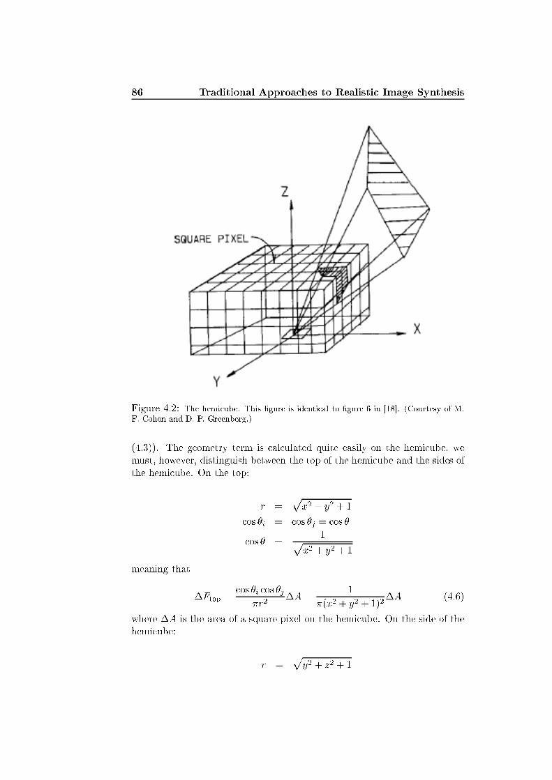
86 Traditional Approa hes to Realisti Image Synthesis

Figure 4.2: The hemi ube. This �gure is identi al to �gure 6 in [18℄. (Courtesy of M.F. Cohen and D. P. Greenberg.)(4.3)). The geometry term is al ulated quite easily on the hemi ube, wemust, however, distinguish between the top of the hemi ube and the sides ofthe hemi ube. On the top: r = px2 + y2 + 1 os �i = os �j = os � os � = 1px2 + y2 + 1meaning that �Ftop = os �i os �j�r2 �A = 1�(x2 + y2 + 1)2�A (4.6)where �A is the area of a square pixel on the hemi ube. On the side of thehemi ube: r = py2 + z2 + 1

4.1 Radiosity 87 os �i = zpy2 + z2 + 1 os �j = 1py2 + z2 + 1meaning that �Fside = os �i os �j�r2 �A = z�(y2 + z2 + 1)2�A (4.7)The hemi ube method enables an implementation of radiosity where pi -tures are taken for ea h fa e of a hemi ube in order to determine form fa torsbetween the re eiving pat h and all other pat hes in the s ene. Taking pi -tures makes it possible to exploit the GPU for radiosity omputations, whi his a great advantage with respe t to pro essing time. The hemi ube methodis the se ond and last form fa tors al ulation method that is in luded inthis proje t.Progressive Re�nementAfter a method for the al ulation of form fa tors has been hosen, a pro-gressive re�nement method is employed in order to solve the system of linearequations given in (4.2). The solution for this system is the radiosity ap-proximation of the illumination that we wish to �nd.Progressive re�nement is an iterative pro ess where ea h iteration repre-sents the propagation of light from the pat h that is urrently the brightest.This orresponds to appli ation of the integral operator Ti ( f. se . 3.6). Forea h iteration Ti is applied to the radiosity of the brightest pat h in the s ene,that is, the brightest pat h distributes its energy to every other pat h in thes ene a ording to the form fa tors between them. An iteration therebysimulates di�use re�e tion o� the brightest pat h.After ea h iteration the radiosity distributed in the s ene is a little loserto the steady state. We an stop the iteration when we see �t, and sin eall obje t materials are perfe tly di�use, the radiosity of a pat h is also theradian e rea hing the eye from that pat h (if the pat h is not o luded).This is also why radiosity solutions are independent of the viewer's positionin the s ene.Having a set of arrays: Final radiosities B, `unshot' radiosities deltaB,emitted radiosities B_e, areas A, and re�e tan es R, holding values for ea hpat h, and moreover a two-dimensional array of form fa tors F holding valuesfor ea h ombination of two pat hes, the C-like pseudo ode for progressivere�nement ould be given as below:for all i{ B[i℄ = B_e[i℄;

88 Traditional Approa hes to Realisti Image SynthesisdeltaB[i℄ = B_e[i℄;}while not onvergen e{ pi k i, su h that deltaB[i℄ * A[i℄ is largest (the brightest pat h);if pat h i has not been visited before{ position hemi ube over pat h i; al ulate form fa tors F[i℄[j℄, j = 1,...,n;}for every pat h j{ temp_deltaB = deltaB[i℄ * R[j℄ * F[i℄[j℄;deltaB[j℄ += temp_deltaB;B[j℄ += temp_deltaB;}deltaB[i℄ = 0;}using a few array theoreti fun tions and the transformer EACH (see de�ni-tion 2) we an rewrite the pseudo ode in a slightly more ompa t form:B := B_e;deltaB := B_e;while not onvergen e{ maxPat h := first sublist [EACH (max (B*A) =), grid℄ (B*A);if maxPat h has not been visited before{ position hemi ube over maxPat h; al ulate the form fa tors of the array (maxPat h pi k rows F);}[B, deltaB℄ := [B, deltaB℄+ [pass, pass℄ ((maxPat h pi k deltaB) * R * (maxPat h pi k rows F));pla e [0 maxPat h, deltaB℄;}where X := Y denotes that ea h element of the array X is assigned the valuefound at the orresponding position in the array Y. A des ription of thearray theoreti fun tions: first, sublist, max, grid, pass, pi k, rows,and pla e an be found in [102℄, the meaning should, however, emerge by omparison to the �rst pseudo ode. The point in having an array theoreti formulation is that the for-loops disappear, whi h reveals the parallel natureof the algorithm. This on ludes our des ription of radiosity. The nextsubje t is lassi ray tra ing.

4.2 Ray Tra ing 894.2 Ray Tra ingThe obje tive of this se tion is to provide a general understanding of themost basi on epts onstituting the global illumination algorithm alledray tra ing.The Basi Con eptThe earliest surviving work on geometri al opti s, written by Eu lid in an- ient times [32℄, initially gives the following des ription of ray tra ing [33℄:Let it be hypothesized that straight lines drawn out from the eyetravel a distan e of large magnitudes,and that the �gure en losed by the sight-lines is a one havingits vertex at the eye and its base at the limits of the things seen,See also �gure 4.3.The �rst re ursive ray tra ing algorithm for omputer graphi s was (asmentioned before) introdu ed by Turner Whitted in 1980 [137℄. Subsequentlymany others have tried to improve and develop this approa h further, stillusing the same basi prin iples.Consider a point light sour e spreading light in all dire tions from a singlepoint in spa e. If the light is divided into rays expe ted to follow straightlines in spa e until they interse t an obje t (as Eu lid hypothesized), ea h ray an be represented by a point of origin, a dire tion ve tor, and a parameterdes ribing how far the light has traversed along the line. Looking at ea hray individually (tra ing ea h ray), gives a method to al ulate how the lightsour e will illuminate a s ene.Ea h time a ray interse ts an obje t some light will be absorbed, somere�e ted and some might be refra ted. This means al ulation of new raysboun ing o� the obje t or passing through it. All rays ought to be fol-lowed until they interse t a Lambertian surfa e (perfe tly di�use surfa e)1,disappear into the ba kground or rea h the eye point.It is easy to imagine that the illumination of a s ene with several obje tsresult in a tremendous amount of rays. On top of that most of the rays arenot even useful to the viewer sin e they never rea h the eye point. In fa tan in�nite number of rays would be needed to illuminate the s ene perfe tly.This is one of the reasons why the pro ess is reversed. Instead of tra ing raysthat depart from the light sour e, rays are tra ed with departure from theeye point (whi h the Greeks in an ient times thought was reality), meaningthat it is only ne essary to tra e rays that a tually have an in�uen e onthe visible area. In that way we an remove the useless rays that do notrea h the eye point anyway. This approa h - al ulating the rays from the1This is the ase in lassi ray tra ing, sin e di�use interre�e tions are not modeled.

90 Traditional Approa hes to Realisti Image Synthesis

Figure 4.3: Eu lid's �The Opti s� is the earliest surviving work on geometri al opti s.There were a number of medieval Latin translations, whi h be ame of new importan ein the �fteenth entury for the theory of linear perspe tive. This te hnique is beautifullyillustrated in the miniature of a street s ene in this elegant manus ript from the libraryof the Duke of Urbino. Text: [32℄. Image: [128℄.eye point instead of the light sour e - is alled forward ray tra ing. Otherapproa hes use rays al ulated from the light sour e or from both, these are alled ba kward ray tra ing and bi-dire tional ray tra ing respe tively. Bothapproa hes are more advan ed than forward ray tra ing, therefore those willnot be onsidered at this point. Forward ray tra ing is pi tured in �gure 4.4.Sin e an eye point, like the point light sour e, is also just a point in spa ean in�nite number of rays ould be tra ed from it in any given dire tion. To�nd the rays that are needed in order to �ll the pi ture of the s ene, a viewplane ( f. se . 2.3) is generated. The ray tra er will ast one or more rays fromthe eye point through ea h pixel of the view plane. When a ray interse ts

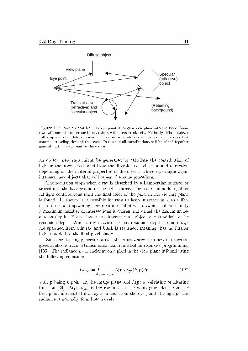
4.2 Ray Tra ing 91

Diffuse object

Specular (reflective) object

View plane

Eye point

Transmisstive (refractive) and specular object

(Returning background) Figure 4.4: Rays are sent from the eye point through a view plane into the s ene. Somerays will never interse t anything, others will interse t obje ts. Perfe tly di�use obje tswill stop the ray while spe ular and transmissive obje ts will generate new rays that ontinue traveling through the s ene. In the end all ontributions will be added togethergenerating the image sent to the s reen.an obje t, new rays might be generated to al ulate the ontribution oflight in the interse ted point from the dire tions of re�e tion and refra tiondepending on the material properties of the obje t. These rays might againinterse t new obje ts that will repeat the same pro edure.The re ursion stops when a ray is absorbed by a Lambertian surfa e, ortra ed into the ba kground or the light sour e. The re ursion adds togetherall light ontributions until the �nal olor of the pixel in the viewing planeis found. In theory it is possible for rays to keep interse ting with di�er-ent obje ts and spawning new rays into in�nity. To avoid that possibilitya maximum number of interse tions is hosen and alled the maximum re- ursion depth. Every time a ray interse ts an obje t one is added to there ursion depth. When a ray rea hes the max re ursion depth no more raysare spawned from this ray and bla k is returned, meaning that no furtherlight is added to the �nal pixel shade.Sin e ray tra ing generates a tree stru ture where ea h new interse tiongives a re�e tion and a transmission leaf, it is ideal for re ursive programming[135℄. The radian e Lpixel in ident on a pixel in the view plane is found usingthe following equation:Lpixel = Zviewplane L(p;!eye)h(p)dp (4.8)with p being a point on the image plane and h(p) a weighting or �lteringfun tion [30℄. L(p;!eye) is the radian e at the point p in ident from the�rst point interse ted if a ray is tra ed from the eye point through p, thisradian e is normally found re ursively:

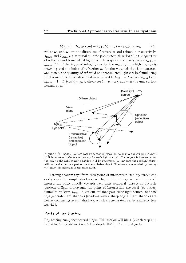
92 Traditional Approa hes to Realisti Image SynthesisL(x;!) = Llo al(x;!) + kre e L(x;!r) + ktransL(x;!t) (4.9)where !r and !t are the dire tions of re�e tion and refra tion respe tively.kre e and ktrans are material spe i� parameters that des ribe the quantityof re�e ted and transmitted light from the obje t respe tively, hen e kre e +ktrans � 1. If the index of refra tion �1 for the material in whi h the ray istraveling and the index of refra tion �2 for the material that is interse tedare known, the quantity of re�e ted and transmitted light an be found usingthe Fresnel re�e tan e des ribed in se tion 3.4: kre e = Fr( os �; �1; �2) andktrans = 1�Fr( os �; �1; �2), where os � = (n �!), and n is the unit surfa enormal at x.

Diffuse object

Specular (reflective) object

View plane

Eye point

Transmisstive (refractive) and specular object

Point light source

Figure 4.5: Shadow rays are ast from ea h interse tion point in a straight line towardsall light sour es in the s ene (one ray for ea h light sour e). If an obje t is interse ted onthe way to the light sour e a shadow will be generated. In this ase the spe ular obje twill ast a shadow on a part of the transmissive obje t. Shadows are generated by leavingout dire t illumination in the al ulation.Tra ing shadow rays from ea h point of interse tion, the ray tra er aneasily al ulate simple shadows, see �gure 4.5. A ray is ast from ea hinterse tion point dire tly towards ea h light sour e, if there is an obsta lebetween a light sour e and the point of interse tion the lo al (or dire t)illumination term Llo al is left out for that parti ular light sour e. Shadowrays generate hard shadows (shadows with a sharp edge). Hard shadows arenot as onvin ing as soft shadows, whi h are generated eg. by radiosity (see�g. 4.1).Parts of ray tra ingRay tra ing omprises several steps. This se tion will identify ea h step andin the following se tions a more in depth des ription will be given.

4.2 Ray Tra ing 93The C-style pseudo ode for a simple ray tra er is given below. It isbuild on the ray tra er implemented in this proje t. Note that the lassi ray tra er supports point light sour es only.Pseudo ode for a simple ray tra er:void tra e_rays() {3Dve tor shade; // RGB olor3Dve tor viewPlaneNormal, viewPlaneU, viewPlaneV, eyePoint;float fo alDistan e;int windowWidth, windowHeight, urrentPosX, urrentPosY;for urrentPosX from 0 to windowWidthfor urrentPosY from 0 to windowHeight{ // Generate ray2Dve tor oords = ( urrentPosX / windowWidth - 0.5, urrentPosY / windowHeight - 0.5);3Dve tor rayDire tion = viewPlaneNormal * fo alDistan e +viewPlaneU * oords[0℄ +viewPlaneV * oords[1℄;r = Ray(eyePoint, normalize(rayDire tion));shade = tra e(r)Send shaded olor to s reen;}}3Dve tor tra e(Ray r) {3Dve tor ba kgroundColor; //RGB olorif r.interse tionCount > MAX_RECURSION_DEPTHshade = BLACK;else{ for i from 0 to numberOfObje tstest for interse tion of i'th obje t with r;3Dve tor interse tedPos = interse tion losest to ray origin;if r interse ts an obje t{ 3Dve tor result = 0;Ray shadowray = spawn ray in dire tion towards the light sour e;tra e(shadowray);if shadowray.did_hit()result += lo al illumination eg. by Phong using the normal,

94 Traditional Approa hes to Realisti Image Synthesisray dire tion, and dire tion to ea h light sour e;// Re ursive refle tionif obje t diffuseness < 1 and obje t refle tivity > 0{ Ray refle t = spawn ray in refle ted dire tion;result += obje t refle titvity * tra e(refle t);}// Re ursive transmissionif obje t transmissivity > 0{ Ray transmit = spawn ray in transmitted dire tion;result += obje t transmissivity * tra e(transmit);}return ( olor of material on interse ted obje t * result);}else return ba kgroundColor;}} Looking at the pseudo ode the di�erent steps of ray tra ing are revealed.First of all the ray tra er must be able to generate rays. When a ray isgenerated there must be dete tion of interse tions, then new rays must bespawn onsidering re�e tion, refra tion and shadows. In the end shading ofthe di�erent interse tion points must be al ulated. This leaves the followinglist of steps that ea h ray must go through:� Ray asting� Interse tion� Re�e tion� Refra tion� ShadingRay CastingThe �rst step in ray tra ing is to generate rays oming from the eye pointthrough a point in the view plane. The view plane represents the pi ture thatwill be ome visible to the user on the s reen. Depending on the demands forimage quality one or more rays an be sent through ea h pixel, as indi atedby the integral in (4.8). Sin e speed of the pro ess very mu h depends onthe number of rays ast less than one ray per pixel an be onsidered ifinterpolation between them is used afterwards.To reate a ray we need a point, a dire tion ve tor, and a distan e param-eter. Initially the point will be the eye point later it will be the interse tion

4.2 Ray Tra ing 95point. The dire tion ve tors of the �rst rays generated are found by drawinga line between the eye point and the point representing a pixel in the view-ing plane (simply by subtra ting one point from the other). All dire tionve tors should be normalized. For a ray spawned at a point of interse tionthe dire tion depends on whether the ray is the result of a re�e tion or arefra tion, see �gure 4.6.

Incoming ray

Reflected ray

Tangent plane

Object

Transmitted ray

θ

θ

α

Figure 4.6: New rays are generated from the interse tion point (unless the obje t is ompletely di�use). For the re�e tive ray the in oming angle � mat hes the outgoingangle. The angle of the transmitted ray � depends on material properties of the obje t.The following equation generates a ray from the eye point. Rays spawnedby re�e tion or transmission are al ulated otherwise ( f. se . 3.1).Let the eye point be given as e = (e0; e1; e2) and a dire tion as:d = [n u v℄24 fuv 35where n, u, and v is an orthonormal frame for the view plane and [f u v℄T isthe fo al distan e and (u; v)- oordinates spe ifying a relative position on theview plane. The ray is then given as the parametri equation of a straightline: r(t) = e+ tdwhere t is the distan e (or time) parameter des ribing how far the light hastraversed along the line. Tra ing a ray, that is, �nding the interse ted pointon the losest visible surfa e along a ray originating at point x and pointingin the dire tion !, an then be des ribed as follows [30℄:

96 Traditional Approa hes to Realisti Image Synthesisr(x;!) = fy : y = x+ tinterse tion!gtinterse tion = minft : t > 0 ^ x+ t! 2 Agwhere all the surfa es in the s ene are represented by the set A. This is alled the ray asting operation.Interse tionInterse tion between rays and obje ts is the heaviest part of the ray tra ingalgorithm. When a ray is tra ed into the s ene there are several things thatmust be onsidered. First step is to �nd out whi h obje ts, if any, the givenray interse ts. In the brute for e manner every ray is he ked for ollisionwith every obje t in the s ene, meaning that interse tion between ea h linerepresenting a ray and every obje t is al ulated. If a ray interse ts morethan one obje t it is ne essary to determine whi h obje t is losest, this isdone using the distan e parameter t (the obje t within the shortest distan eis, of ourse, the losest and the one interse ted).It is obvious that brute for e testing is quite omputationally expensive,espe ially if the obje ts have a omplex stru ture. To help this, obje tsare usually de�ned as ombinations of primitives for whi h we an moreeasily ompute interse tions. Besides ea h obje t an be surrounded by abounding box, whi h is a box �tted to surround the obje t tightly. Whenrays are tra ed through the s ene they �rst he k for interse tions with thebounding boxes, whi h is less omplex than al ulation of interse tion withea h triangle in the s ene. In this way all the obje ts residing in a box thatis not hit by a ray an be left out of the interse tion al ulations, see �gure4.7.Sin e obje ts are onstru ted from primitives, we only have to implement ollision dete tion with the primitives represented in our s ene. In prin iplethe only primitives we need are a triangle and the shape of the primitiveused as bounding volume (in most ases a box). Other primitives that arefrequently used in omputer graphi s are spheres, ones, planes and toruses(see �g. 7.1). The equations that provide interse tion between a line and asphere, a triangle, a box, or a plane are provided later in this se tion.When the ray interse ts, the next step is to generate a re�e ted rayand a transmitted ray, depending on material properties. If the obje t isperfe tly di�use there will be no re�e ted ray or transmitted ray, otherwisethe ontribution of light from the re�e ted and transmitted rays depend onthe re�e tivity, kre e , and transmissivity, ktrans, parameters of the obje tmaterial, or more orre tly it depends on the Fresnel re�e tan e given bythe refra tion indi es of the di�erent media through whi h the ray travels.

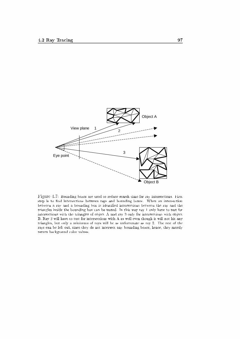
4.2 Ray Tra ing 97

View plane

Eye point

Object A

Object B

1 2

3

Figure 4.7: Bounding boxes are used to redu e sear h time for ray interse tions. Firststep is to �nd interse tions between rays and bounding boxes. When an interse tionbetween a ray and a bounding box is identi�ed interse tions between the ray and thetriangles inside the bounding box an be tested. In this way ray 1 only have to test forinterse tions with the triangles of obje t A and ray 3 only for interse tions with obje tB. Ray 2 will have to test for interse tions with A as well even though it will not hit anytriangles, but only a minimum of rays will be as unfortunate as ray 2. The rest of therays an be left out, sin e they do not interse t any bounding boxes, hen e, they merelyreturn ba kground olor values.

98 Traditional Approa hes to Realisti Image SynthesisIf a ray hits a Lambertian surfa e or is tra ed into the ba kground, there ursion stops. This is the end point of the re ursive pattern. When anend point is rea hed an RGB olor value is returned a ording to the olorof the Lambertian surfa e or the ba kground olor. Moreover the end pointwill return no olor (bla k) if the maximum re ursion depth is rea hed. All ontributions are added together all the way up to the view plane represent-ing the pixels that are sent to the output window on the s reen. Ea h timea ontribution from a re�e ted or transmitted ray is added to the total on-tributions the values are multiplied by a per entage fa tor, representing there�e tion or transmission fa tor of the obje t. The result is that the higherthe re ursion depth the less the ontribution to the �nal pixel shade.Ray/Sphere Interse tionConsider a ray represented by a straight line r(t):r(t) = o+ tdwhere t is a parameter indi ating the distan e traversed from the origin oalong the line in dire tion d. r(t) is then a position in spa e that oin ideswith the line. A sphere with the enter positioned at = ( x; y; z) andwith a radius r is represented by the following equation:(x� x)2 + (y � y)2 + (z � z)2 = r2or jj(x; y; z) � ( x; y; z)jj � r = 0 ) jjr(t)� jj � r = 0This simpli�es to [2, p. 569℄.t2 + 2tb+ = 0where b = d � (o� ) and = (o� ) � (o� )� r2.Solving the quadrati equation above gives the following points of in-terse tion between the ray and the sphere, if b2 � , else no interse tionsexist: t = �b�pb2 � The ray tra er is only on erned with the �rst point interse ted along theline (the smallest t value of interse tion greater than zero). Therefore, if theray origin is outside the sphere, we hoose the interse tion t = �b�pb2 � ,otherwise t = �b+pb2 � is the orre t point of interse tion. In ase the rayis tangent to the sphere there will be only one point of interse tion t = �b.

4.2 Ray Tra ing 99Ray/Triangle Interse tionCon erning polygons we have hosen, in the standard ray tra er, to imple-ment ray/triangle interse tion only. Most s enes in lude only polygons ofthree and four verti es (triangles and quadrilaterals), and a polygon of fourverti es easily simpli�es to two triangles.A point, t(u; v) on a triangle, spanned by the verti es v0, v1 and v2, isgiven by the following equation:t(u; v) = (1� u� v)v0 + uv1 + vv2where u � 0, v � 0, and u + v � 1. u, v, and w = 1 � u � v are alledbary entri oordinates for the triangle (see eg. [42℄).Solving the equation r(t) = t(u; v) gives the point of interse tion, if any.Denoting e1 = v1 � v0, e2 = v2 � v0, and s = o� v0 the solution �nding t,u, and v is [2, p. 580℄:0� tuv 1A = 1(d� e2) � e1 0� (s� e1) � e2(d� e2) � s(s� e1) � d 1ARay/AABB OverlapAABB is short for Axis Aligned Bounding Box. When testing rays againstbounding volumes it is only ne essary to determine whether there is an in-terse tion or not, the exa t interse tion point is not required, sin e the raywill be tested against the primitives ontained within the bounding volumesubsequently. This simpli�es the al ulation onsiderably.Sin e light only travels in one dire tion along the line representing theray, we are looking at the interval [0;1[ or, hoosing a large �oating pointvalue to represent in�nity, t 2 [0; 106℄ = [tmin; tmax℄.Consider an AABB des ribed by a two points pmin and pmax and a linesegment representing the ray that we wish to test for overlap also des ribedby two points rmin(tmin) and rmax(tmax). Let h = (hx; hy; hz) = (pmax �pmin)=2 denote the half ve tor of the bounding box, let = ( x; y; z) =(rmax(tmax) + rmin(tmin))=2 denote enter of the line segment, and let w =(wx; wy; wz) = rmax(tmax) � denote the half ve tor of the line segment,then the following test will de ide whether the ray overlaps the axis alignedbounding box or not [2℄: j xj > vx + hx^ j yj > vy + hy^ j z j > vz + hz^ j ywz � zwyj > hyvz + hzvy

100 Traditional Approa hes to Realisti Image Synthesis^ j xwz � zwxj > hxvz + hzvx^ j xwy � ywxj > hxvy + hyvxwhere (vx; vy; vz) = (jwxj; jwy j; jwz j). If this holds true the ray overlaps thebounding box, otherwise the ray and the AABB are disjoint.Ray/Plane Interse tionThough planes are usually not present in real-time omputer graphi s, sin erendering obje ts of in�nite size is ine� ient, we will in lude them in ourray tra er as the rays are tra ed into in�nity anyway.The interse tion point between a line r(t) representing a ray and a plane,des ribed by a normal n and a point p in the plane, is found solving thefollowing equation:n � (r(t)� p) = 0 ) t = �n � p+n � on � d ; n � d 6= 0If n � d = 0 the ray and the plane are parallel.Re�e tionThe re�e ted ray is a new ray generated at a point of interse tion. Theray has the exa t same properties as any other ray. As mentioned before aray has a ve tor des ribing its dire tion and a parameter t telling how farthe light has traversed along the line. The dire tion of a re�e ted ray isdetermined by the law of re�e tion (see se . 3.1). You ould say that there�e ted ray is a mirrored image of the in oming ray through the normal nof the interse ted surfa e in the plane of in iden e, see �gures 4.6 and 3.3.(3.2) an be used to �nd the dire tion of the re�e ted ray dr. For onve-nien e we repeat the equation below:dr = 2(d0 � n)n� d0where d0 = �d is the dire tion from the point of interse tion towards theray origin.Refra tion (or Transmission)The transmitted ray is the ray refra ted through a transparent material. Thedire tion of the transmitted ray depends on obje t material properties andthe angle between the normal n and the dire tion d of the in ident ray. Thetransmissivity of the material states the per entage of the in oming light thatis transmitted. Furthermore the ratio �1=�2 between the index of refra tion�1 for the material in whi h the in ident ray was travelling and the index of

4.3 Monte Carlo Ray Tra ing 101refra tion �2 for the material whi h the ray is refra ted into, has an in�uen eon the dire tion of the refra ted ray.The dire tion dt of a transmitted ray an be found using equation (3.5),whi h is repeated below:dt = �1�2 ((d0 � n)n� d0)� ns1���1�2�2 (1� (d0 � n)2)where again d0 = �d is the dire tion from the point of interse tion towardsthe ray origin.ShadingThe �nal shade of ea h pixel is found when the re ursive algorithm unravels,meaning that ea h pixel shade is found adding up the ontribution from allthe rays that was spawned at ea h point of interse tion when that parti ularray was tra ed into the s ene from the eye point through a pixel in the view-plane. Lo al illumination is al ulated at ea h point of interse tion usingsome kind of BRDF (eg. Phong).Sending the �nal pixel olor to the s reen is arried out using a graphi slibrary su h as OpenGL or Dire t3D.The next se tion is a short presentation of Monte Carlo ray tra ing.Monte Carlo ray tra ing is a ne essary step in the dire tion towards photonmapping. Monte Carlo te hniques are also very useful in their own right,they are unfortunately often also quite omputationally expensive.4.3 Monte Carlo Ray Tra ingAs shortly des ribed in se tion 3.8, point sampling is one of the two basi te hniques that an be used in order to solve a re ursive integral su h as therendering equation. Mathemati al te hniques that use statisti al samplingto simulate phenomenon or evaluate values of fun tions are alled MonteCarlo te hniques [30℄.Suppose we want to evaluate the following integral using a Monte Carlomethod: I = Zx f(x)dxwhere x is a possibly multi-dimensional variable with domain x. Then aMonte Carlo estimator hIi will approximate I by taking a lot of randomsamples, g(xi) ; x 2 x ; i = 1; : : : ; N , and averaging their ontributions[126℄: hIi = 1N NXi=1 g(xi) = 1N NXi=1 f(xi)p(xi)

102 Traditional Approa hes to Realisti Image Synthesiswhere p(xi) is a probability density fun tion (PDF) a ording to whi h we an draw samples. If all N random variables have the same PDF they are alled independent identi ally distributed (IID) variables. In [30, p. 57℄ it isshown that if all N variables are IID variables, the expe ted value (or themean) of the estimator E[hIi℄ equals the desired integral I. The varian e ofthis estimator is given as:�2 = 1N Z �f(x)p(x) � I�2 p(x)dxmeaning that the varian e de reases linearly as N in reases. The standarddeviation � is the square root of the varian e, whi h means that in orderto halve the error in the estimator E[hIi℄ we must quadruple the number ofsamples. This is the reason for slow onvergen e of Monte Carlo ray tra ing.General properties of the PDF are:8x : p(x) � 0Z 1�1 p(x)dx = 1The remaining problem, before we are able to use the Monte Carlo te h-nique for approximation of the rendering equation, is that we must be ableto sample a ording to the PDF that we see �t. In [30, p. 64℄ it is explainedhow this is done: �A sample an be generated a ording to a given distri-bution p(x) by applying the inverse umulative distribution fun tion of p(x)to a uniformly generated random variable� � over the interval2 [0; 1[. The umulative distribution fun tion (CDF) is de�ned as [30℄:P (y) = Pr(x � y) = Z y�1 p(x)dxLooking at the integral al ulating re�e ted radian e in (3.53) it wouldbe onvenient to be able to sample a ording to a osine PDF:p(�; �) = os��where � and � are spheri al oordinates.The umulative distribution fun tion P (�; �) is derived in [30, p. 66℄:P (�; �) = �2� (1� os2 �)2We use the notation [a; b[, instead of [a; b) to denote that b is not in luded in theinterval.

4.3 Monte Carlo Ray Tra ing 103whi h is separable with respe t to � and �, resulting in the following formulafor omputing the spheri al oordinates of a dire tion sampled a ording tothe osine PDF: (�; �) = � os�1(p�0); 2��1� (4.10)where �i 2 [0; 1[ ; i = 0; 1. (With respe t to the derivation of (4.10) fromthe CDF it should be noted in the ase of � that �1 repla es 1� �, whi h ispossible sin e � 2 [0; 1[.)A few other distributions useful for rendering are given in [124, p. 33℄.Being able to sample a ording to the osine lobe by al ulation of newdire tions using (4.10), we an for example expand the ray tra ing des ribedin the previous se tion by adding a radian e term Lindire t to (4.9). Lindire tsimulates multiple di�use re�e tions:L(x;!) = Llo al(x;!) + kre e L(x;!r) + ktransL(x;!t)+(1� kre e � ktrans)Lindire t(x;!) (4.11)In order to al ulate the indire t illumination term N sample rays aretra ed with dire tions !i ; i = 1; : : : ; N found using (4.10). Lindire t is esti-mated using the following Monte Carlo estimator:hLindire ti = �dN XL(x;!i) (4.12)where �d is the di�use re�e tan e. This estimator follows sin e p(x) = os �=� = (! � n)=�, and sin e:fr(x;!;!0) = fr = �d�when the material is perfe tly di�use, with a onstant di�use re�e tan e.The above expansion of lassi ray tra ing e�e tively makes ray tra ingable to model di�use interre�e tions. The onvergen e is, however, slow.Many sample rays must be distributed and tra ed re ursively in order to ob-tain a de ent evaluation of the indire t illumination term. Photon mapping,whi h is the subje t of the next se tion, presents a method that signi� antly an speed up the al ulation of the indire t illumination term in Monte Carloray tra ing.Another appli ation of of the Monte Carlo te hnique is that it enables omplex light sour es (that is, light sour es with an areal extension) in raytra ing. In the ase of omplex light sour es the dire t illumination term(Llo al in (4.11)) should be evaluated using a Monte Carlo estimator samplingseveral rays towards random positions on ea h light sour e.In order to have a renderer that an simulate full global illumination we hoose to implement photon mapping, whi h is the subje t of the followingse tion.

104 Traditional Approa hes to Realisti Image Synthesis4.4 Photon MappingRe all He kbert's idea of adaptive radiosity textures (se tion 3.7). He kbertdes ribes a two-pass method in whi h photons are emitted from light sour es,stored in �radiosity textures�, and re-emitted from the brightest surfa e in aprogressive re�nement manner to a ount for the light paths: L(S*D)*, andrays are emitted from the eye point to a ount for the paths DS*E.Photon mapping is a similar kind of two-pass method. The most impor-tant di�eren e is that when a photon interse ts a di�use surfa e it is stored ina map whi h is independent of the s ene geometry. Instead of the progressivere�nement approa h for modeling multiple di�use re�e tions, ea h photon istra ed through the s ene using Russian roulette (see the following se tion onphoton tra ing). Sin e the resulting photon map is independent of geometrywe an not use textures for radian e estimates when ray tra ing the s enefrom the eye point. Instead the rendering equation must be approximatedby a radian e estimate, whi h is based on the density of photons over a givensurfa e area. All in all photon mapping omprises the following steps:� Photon tra ing1. Photon emission.2. Photon s attering.3. Photon storing� Forward ray tra ing� The radian e estimateEa h of these steps will be addressed in the following. Our presentationbasi ally follows [60℄. Photon mapping in its purest form raves an immensenumber of photons in order to give a good radian e estimate. After thepresentation of the steps given above, we will therefore brie�y des ribe howphoton mapping an be ombined with other te hniques (eg. distribution raytra ing) in order to lower the number of photons needed for an a eptableresult. In ombination with other methods photon mapping is speeded upsigni� antly. The low pro essing time ombined with the independen e ofgeometry and the ompatibility with rendering of parti ipating media ur-rently makes photon mapping one of the most powerful te hniques simulatingfull global illumination.Photon Tra ingPhotons are tra ed as ordinary rays. They are tra ed from the light sour eas in ba kward ray tra ing. The di�eren e lies in how they are s atted andstored in the photon map when interse ting a material. Photon mapping usesa sto hasti method rather than the re ursive method used in ray tra ing.

4.4 Photon Mapping 105Photon EmissionPhoton mapping an simulate any type of light sour e. The reason is thesto hasti method that photon mapping employs. Ea h photon is emit-ted from a random lo ation on a light sour e in a random dire tion. Onemethod to use for �nding random dire tions is reje tion sampling, whi h usesrepeated evaluation of random numbers until a ertain property is present.An example is an isotropi point light sour e emitting light uniformly in alldire tions. The reje tion sampling pi k random samples in the unit ubeand if the sample is also inside the unit sphere it is normalized and used asa dire tion for an emitted photon.Having three random variables �i 2 [0; 1℄ ; i = 0; 1; 2 the following C-likepseudo ode implements photon emission:int n_e = 0; // number of photons emittedwhile(not enough photons){ do{ x = 2*xi_0 - 1;y = 2*xi_1 - 1;z = 2*xi_2 - 1;}while(x*x + y*y + z*z > 1);3Dve tor d = normalize(3Dve tor(x, y, z));3Dve tor p = random lo ation on light sour e;tra e photon from p in dire tion d;n_e++;}s ale power of photons with 1/n_e;As noted, the power of the photons should be s aled a ording to thenumber of photons that have been emitted, whi h is most probably not thesame as the number of photons stored in the photon map.Photon S atteringThe basi idea of photon s attering is to importan e sample a single dire tionof re�e tion a ording to the BRDF (or BTDF in ase of transmission), asopposed to distribution ray tra ing where numerous rays are spawned at ea hinterse tion. The photon may also be absorbed. In that ase the re ursionstops.When a photon interse ts an obje t, the type of intera tion is de idedby the material properties. One way to de ide the type of interse tion is asfollows. Consider a material having di�use re�e tan e (�d;r; �d;g; �d;b) andspe ular re�e tan e (�s;r; �s;g; �s;b), where r, g, and b denotes the three olor

106 Traditional Approa hes to Realisti Image Synthesisbands: red, green, and blue. The type of intera tion is hosen using Russianroulette (�rst introdu ed to omputer graphi s by Arvo and Kirk [5℄). Firstthe average di�use re�e tan e �d;avg and the average spe ular re�e tan e�s;avg is determined: �d;avg = �d;r + �d;g + �d;b3�s;avg = �s;r + �s;g + �s;b3Then having a uniformly distributed random variable � 2 [0; 1℄, the Rus-sian roulette works as follows:� 2 [0; �d;avg℄ �! di�use re�e tion� 2℄�d;avg; �s;avg + �d;avg℄ �! spe ular re�e tion� 2℄�s;avg + �d;avg; 1℄ �! absorption(here we use the notation ℄a; b℄, instead of (a; b℄, to denote that a is notin luded in the interval.)If the photon is re�e ted, the power of the re�e ted photon is s aleda ording to the spe tral re�e tan e value:�r = �i;r�r=�avg�g = �i;g�g=�avg�b = �i;b�b=�avgwhere the i subs ript denotes the spe tral power of the in ident photon.� and �avg are either di�use or spe ular re�e tan e values, whi h kind to hoose depends on the result of the Russian roulette.The re�e ted photon will be tra ed in a dire tion sampled a ording tothe BRDF. If the re�e tion is spe ular another Russian roulette an be usedto hoose whether the photon is re�e ted or transmitted:� 2 [0; Fr℄ �! spe ular re�e tion� 2℄Fr; 1℄ �! spe ular refra tionwhere Fr is the Fresnel re�e tan e (see (3.35), (3.36), and (3.37)).In ase of spe ular refra tion the dire tion is sampled a ording to aBTDF rather than a BRDF.If the material is perfe tly spe ular, the photon will be tra ed in thedire tion given by (3.2) or (3.5) depending on the result of the Russianroulette.

4.4 Photon Mapping 107If di�use re�e tion is the result of the Russian roulette, and if the materialis perfe tly di�use, the re�e ted dire tion �is found by pi king a randomdire tion on the hemisphere above the interse tion point with a probabilityproportional to the osine of the angle with the normal� [60, p. 61℄. Havingtwo uniformly distributed random variables �i 2 [0; 1[ ; i = 0; 1, the dire tionis found in spheri al oordinates a ording to (4.10):(�; �) = � os�1(p�0); 2��1�The reason why the osine lobe is used instead of eg. reje tion samplingis that the re�e ted samples will be weighted by the osine term that alsoappears in the rendering equation.Photon StoringWhenever a photon interse ts a di�use surfa e (not ne essarily perfe tlydi�use) it is stored in the photon map. The radian e estimate that an beobtained from a photon map is mu h too in orre t for the single re�e teddire tion of perfe tly spe ular materials, therefore lassi forward ray tra ingis used for spe ular re�e tions (re all the se ond pass from the eye a ountingfor the paths DS*E).When a photon is stored it represents �ux in ident on a surfa e. Allthe photons are stored in a kd-tree, see se tion 2.5. For a more thoroughdes ription of the kd-tree for photon mapping we refer to [60, hap. 6℄ and to[44℄ in whi h they show improved results with respe t to the kd-tree. Otherspatial data stru tures ould be used as well, as mentioned in se tion 2.5Günther et al [44℄ also report good results with a uniform grid of voxels forthe photon map data stru tureForward Ray Tra ingThe pass from the eye happens exa tly as des ribed in se tion 4.2. Theonly thing that should be noted is that Llo al in (4.9) should be repla edby Lglobal, sin e the radian e estimate des ribed in the following makes itpossible to simulate full global illumination.The Radian e EstimateIn order to al ulate an estimate of Lglobal using the photon map, the render-ing equation must be rewritten in terms of �ux in ident on a surfa e. (3.24),from whi h the rendering equation was derived, states the following, if weintegrate on both sides of the equation:Lr(x;!) = Z fr(x;!;!0)dEi

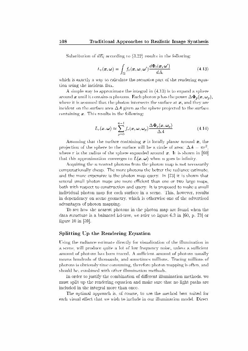
108 Traditional Approa hes to Realisti Image SynthesisSubstitution of dEi a ording to (3.22) results in the following:Lr(x;!) = Z fr(x;!;!0)d�i(x;!0)dAi (4.13)whi h is exa tly a way to al ulate the re ursive part of the rendering equa-tion using the in ident �ux.A simple way to approximate the integral in (4.13) is to expand a spherearound x until it ontains n photons. Ea h photon p has the power��p(x;!p),where it is assumed that the photon interse ts the surfa e at x, and they arein ident on the surfa e area �A given as the sphere proje ted to the surfa e ontaining x. This results in the following:Lr(x;!) � n�1Xp=0 fr(x;!;!p)��p(x;!p)�A (4.14)Assuming that the surfa e ontaining x is lo ally planar around x, theproje tion of the sphere to the surfa e will be a ir le of area: �A = �r2,where r is the radius of the sphere expanded around x. It is shown in [60℄that this approximation onverges to L(x;!) when n goes to in�nity.A quiring the n nearest photons from the photon map is not ne essarily omputationally heap. The more photons the better the radian e estimate,and the more expensive is the photon map query. In [73℄ it is shown thatseveral small photon maps are more e� ient than one or two large maps,both with respe t to onstru tion and query. It is proposed to make a smallindividual photon map for ea h surfa e in a s ene. This, however, resultsin dependen y on s ene geometry, whi h is otherwise one of the advertisedadvantages of photon mapping.To see how the nearest photons in the photon map are found when thedata stru ture is a balan ed kd-tree, we refer to �gure 6.3 in [60, p. 73℄ or�gure 10 in [59℄.Splitting Up the Rendering EquationUsing the radian e estimate dire tly for visualization of the illumination ina s ene, will produ e quite a lot of low-frequen y noise, unless a su� ientamount of photons has been tra ed. A su� ient amount of photons usuallymeans hundreds of thousands, and sometimes millions. Tra ing millions ofphotons is obviously time onsuming, therefore photon mapping is often, andshould be, ombined with other illumination methods.In order to justify the ombination of di�erent illumination methods, wemust split up the rendering equation and make sure that no light paths arein luded in the integral more than on e.The optimal approa h is, of ourse, to use the method best suited forea h visual e�e t that we wish to in lude in our illumination model. Dire t

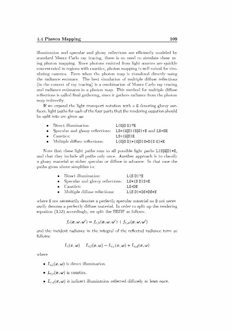
4.4 Photon Mapping 109illumination and spe ular and glossy re�e tions are e� iently modeled bystandard Monte Carlo ray tra ing, there is no need to simulate these us-ing photon mapping. Sin e photons emitted from light sour es are qui kly on entrated in regions with austi s, photon mapping is well suited for sim-ulating austi s. Even when the photon map is visualized dire tly usingthe radian e estimate. The best simulation of multiple di�use re�e tions(in the ontext of ray tra ing) is a ombination of Monte Carlo ray tra ingand radian e estimates in a photon map. This method for multiple di�usere�e tions is alled �nal gathering, sin e it gathers radian e from the photonmap indire tly.If we expand the light transport notation with a G denoting glossy sur-fa es, light paths for ea h of the four parts that the rendering equation shouldbe split into are given as:� Dire t illumination: L(SjGjD)?E� Spe ular and glossy re�e tions: LS*(GjD)(SjG)+E and LS+SE� Causti s: LS+(GjD)E� Multiple di�use re�e tions: L(SjGjD)*(GjD)S*D(SjG)*ENote that these light paths sum to all possible light paths L(SjGjD)*E,and that they in lude all paths only on e. Another approa h is to lassifya glossy material as either spe ular or di�use in advan e. In that ase thepaths given above simpli�es to:� Dire t illumination: L(SjD)?E� Spe ular and glossy re�e tions: LS*(SjD)S+E� Causti s: LS+DE� Multiple di�use re�e tions: L(SjD)*DS*DS*Ewhere S not ne essarily denotes a perfe tly spe ular material an D not ne es-sarily denotes a perfe tly di�use material. In order to split up the renderingequation (3.53) a ordingly, we split the BRDF as follows:fr(x;!;!0) = fr;S(x;!;!0) + fr;D(x;!;!0)and the in ident radian e in the integral of the re�e ted radian e term asfollows: Li(x;!) = Li;l(x;!) + Li; (x;!) + Li;d(x;!)where� Li;l(x;!) is dire t illumination.� Li; (x;!) is austi s.� Li;d(x;!) is indire t illumination re�e ted di�usely at least on e.

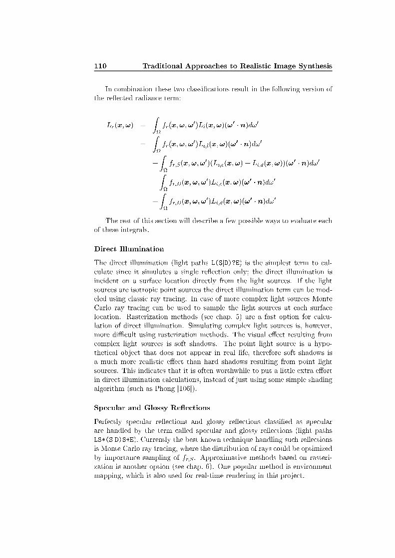
110 Traditional Approa hes to Realisti Image SynthesisIn ombination these two lassi� ations result in the following version ofthe re�e ted radian e term:Lr(x;!) = Z fr(x;!;!0)Li(x;!)(!0 � n)d!0= Z fr(x;!;!0)Li;l(x;!)(!0 � n)d!0+Z fr;S(x;!;!0)(Li; (x;!) + Li;d(x;!))(!0 � n)d!0+Z fr;D(x;!;!0)Li; (x;!)(!0 � n)d!0+Z fr;D(x;!;!0)Li;d(x;!)(!0 � n)d!0The rest of this se tion will des ribe a few possible ways to evaluate ea hof these integrals.Dire t IlluminationThe dire t illumination (light paths L(SjD)?E) is the simplest term to al- ulate sin e it simulates a single re�e tion only; the dire t illumination isin ident on a surfa e lo ation dire tly from the light sour es. If the lightsour es are isotropi point sour es the dire t illumination term an be mod-eled using lassi ray tra ing. In ase of more omplex light sour es MonteCarlo ray tra ing an be used to sample the light sour es at ea h surfa elo ation. Rasterization methods (see hap. 5) are a fast option for al u-lation of dire t illumination. Simulating omplex light sour es is, however,more di� ult using rasterization methods. The visual e�e t resulting from omplex light sour es is soft shadows. The point light sour e is a hypo-theti al obje t that does not appear in real life, therefore soft shadows isa mu h more realisti e�e t than hard shadows resulting from point lightsour es. This indi ates that it is often worthwhile to put a little extra e�ortin dire t illumination al ulations, instead of just using some simple shadingalgorithm (su h as Phong [106℄).Spe ular and Glossy Re�e tionsPerfe tly spe ular re�e tions and glossy re�e tions lassi�ed as spe ularare handled by the term alled spe ular and glossy re�e tions (light pathsLS*(SjD)S+E). Currently the best known te hnique handling su h re�e tionsis Monte Carlo ray tra ing, where the distribution of rays ould be optimizedby importan e sampling of fr;S. Approximative methods based on rasteri-zation is another option (see hap. 6). One popular method is environmentmapping, whi h is also used for real-time rendering in this proje t.

4.4 Photon Mapping 111Causti sAs mentioned before austi s an be simulated by a dire t visualization ofthe photon map. In fa t this approa h is on urrently the most su essfulapproa h to simulation of austi s. In order to evaluate the austi s term(light paths LS+DE) individually, only photons that have taken the paths LS+Dare stored in a separate austi s photon map. Radian e estimates using thismap is an a eptable evaluation of the austi s term. Only few rasterizationmethods exist for austi s, one is presented in [130℄.Multiple Di�use Re�e tionsThe multiple di�use re�e tions term (light paths L(SjD)*DS*DS*E) simulatesthe e�e ts that we also see in radiosity (an example is �g. 4.1) and thensome. No doubt this term is the part of the rendering equation that is most ostly to evaluate. Monte Carlo ray tra ing ould be used to evaluate thisterm, this would, however, be unne essarily time onsuming. A separatephoton map ontaining only photons that have taken the paths L(SjD)*DS*D ould be used for the evaluation of the term, this, however, often resultsin low-frequen y noise. The ombination of the two methods is an e� ientalternative, whi h is alled �nal gathering.Final gathering evaluates the multiple di�use re�e tions term using aglobal photon map ontaining all stored photons (light paths L(SjD)*D). Theglobal photon map is not dire tly visualized, instead the light paths DS*DS*Eare simulated by Monte Carlo ray tra ing. This means that a ray tra edfrom the eye rea hing a di�use surfa e will evaluate the multiple di�use re-�e tions term by sample rays distributed over the hemisphere a ording tofr;D. When a sample ray rea h another di�use surfa e a radian e estimatefrom the global photon will be used to simulate the remaining part of thelight path. Compared to the approa h that dire tly visualizes a photon map ontaining only photons re�e ted di�usely at least on e, this approa h dra-mati ally de reases the amount of photons needed for the radian e estimatein order to get a de ent result. The sampling, however, in reases the timeneeded for the omputation.In part III we des ribe a rasterization approa h that partly simulatesthe multiple di�use re�e tions term. Our method simulate the light pathsLS*DDS*E using a map storing dire t illumination from the light sour e (andpossibly some spe ular re�e tions, that is, light paths LS*D), therefore it is alled dire t radian e mapping.The des ription of the di�erent terms have ea h referred to rasterizationmethods that an give an approximate evaluation of the integrals. In orderto appre iate su h approa hes the traditional approa h to real-time render-ing, whi h is based on rasterization, will be presented in the next hapter.The extensions (su h as those referred to in this se tion) that brings the ras-

112 Traditional Approa hes to Realisti Image Synthesisterization approa h loser to a better evaluation of the rendering equationwill be des ribed in hapter 6.

Chapter 5Traditional Approa hes toReal-Time Rendering

The art of life is a onstant readjustment to our surroundings.Kakuzo Okakura

114 Traditional Approa hes to Real-Time RenderingWhile photorealisti rendering has its main fo us on orre tness of the s eneand for the rendering to be ome as lose to the real world as possible, theabsolute main issue in real-time rendering is the pro essing time needed forea h rendering. Methods for real-time rendering are very mu h limited dueto this issue. Pro essing time is also the main reason why real-time ren-dering traditionally is based on lo al illumination and rasterization ratherthan global illumination methods su h as ray tra ing or radiosity. Photore-alisti e�e ts in real-time are often based on a very simpli�ed version of themathemati s and physi al laws behind the lighting al ulations. Sometimesreal-time methods even do not onsider the physi s behind a visual e�e t, in-stead they simply fake the e�e t using whatever model that makes the resultlook right. This approa h is not ne essarily bad, but in this proje t we haveemphasis on physi al realism. In this hapter we will therefore seek to de-s ribe how traditional methods for real-time rendering works and what theirlimitations are with respe t to visual realism. In hapter 6 we will des ribehow di�erent expansions of the real-time rendering on ept approa hes abetter evaluation of the rendering equation.The �rst se tion of this hapter (5.1) will in short des ribe the pipelineof real-time rendering.Having the pipeline at hand, it is des ribed in se tion 5.2 how obje ts areusually lighted and shaded in real-time and at whi h stage in the pipelinethis usually takes pla e.In se tion 5.3 it is des ribed how textures are used to indulge visualrealism into a rasterized image. When an obje t is textured it means thatan image is `glued' onto the obje t.This on ludes a relatively short hapter on traditional real-time render-ing. The reason why we do not go into spe i� details on algorithms andte hniques for a omplete implementation of the rendering pipeline is thatmost of the te hniques ne essary for traditional real-time rendering are im-plemented in hardware today. This means that everything needed in orderto implement traditional real-time rendering is a graphi s library su h asOpenGL or Dire t3D. The graphi s libraries exploit a GPU if its availableand otherwise they simulate the standard te hniques in software.5.1 The Graphi s Rendering PipelineInitially we an divide the rendering pipeline into three on eptual stages:An appli ation stage, a geometry stage, and a rasterizer stage [2℄, see �gure5.1. Ea h of these stages may itself onstitute a pipeline. In the followingwe will des ribe ea h of the on eptual stages.

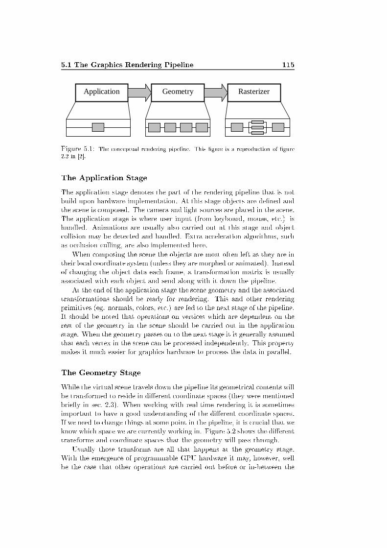
5.1 The Graphi s Rendering Pipeline 115

Application Geometry Rasterizer

Figure 5.1: The on eptual rendering pipeline. This �gure is a reprodu tion of �gure2.2 in [2℄.The Appli ation StageThe appli ation stage denotes the part of the rendering pipeline that is notbuild upon hardware implementation. At this stage obje ts are de�ned andthe s ene is omposed. The amera and light sour es are pla ed in the s ene.The appli ation stage is where user input (from keyboard, mouse, et .) ishandled. Animations are usually also arried out at this stage and obje t ollision may be dete ted and handled. Extra a eleration algorithms, su has o lusion ulling, are also implemented here.When omposing the s ene the obje ts are most often left as they are intheir lo al oordinate system (unless they are morphed or animated). Insteadof hanging the obje t data ea h frame, a transformation matrix is usuallyasso iated with ea h obje t and send along with it down the pipeline.At the end of the appli ation stage the s ene geometry and the asso iatedtransformations should be ready for rendering. This and other renderingprimitives (eg. normals, olors, et .) are fed to the next stage of the pipeline.It should be noted that operations on verti es whi h are dependent on therest of the geometry in the s ene should be arried out in the appli ationstage. When the geometry passes on to the next stage it is generally assumedthat ea h vertex in the s ene an be pro essed independently. This propertymakes it mu h easier for graphi s hardware to pro ess the data in parallel.The Geometry StageWhile the virtual s ene travels down the pipeline its geometri al ontents willbe transformed to reside in di�erent oordinate spa es (they were mentionedbrie�y in se . 2.3). When working with real-time rendering it is sometimesimportant to have a good understanding of the di�erent oordinate spa es.If we need to hange things at some point in the pipeline, it is ru ial that weknow whi h spa e we are urrently working in. Figure 5.2 shows the di�erenttransforms and oordinate spa es that the geometry will pass through.Usually those transforms are all that happens at the geometry stage.With the emergen e of programmable GPU hardware it may, however, wellbe the ase that other operations are arried out before or in-between the

116 Traditional Approa hes to Real-Time Rendering

Object Space

Modeling Transform

World Space

Viewport and Depth Range Transform

Perspective Divide

Projection Transform

View Transform

Clip Space

Normalized Device Space

Eye Space

Window Space Figure 5.2: The di�erent transforms that will be applied to the geometry and thedi�erent oordinate spa es that it will reside in while passing through the geometry stageof the rendering pipeline. This �gure is a reprodu tion of �gure 4-1 in [36℄transforms. The part of the geometry pipeline that has been made pro-grammable is the transition from obje t spa e to lip spa e in �gure 5.2. Ifwe hoose to re-program the vertex pro essor (whi h this part of the pipelineis alled in GPU terminology), we must keep in mind that modeling, view,and proje tion transformations are repla ed by the vertex program we re-ate. Therefore, if we want the pipeline to behave as usual after adding ourmodi� ations to the vertex pro essor, we must remember to arry out thesetransformations in our vertex program. The di�erent transformations aredes ribed in the following.Modeling TransformEa h vertex is given in homogenous oordinates ( f. se . 2.3). The modelingtransform is any kind of transformation that the appli ation stage has founduseful. An obje t might have been modeled around the origin of its lo al oordinate system and the modeling transform an spe ify whi h positionand orientation the obje t should have in world spa e. In this way themodeling transform an also spe ify movement of obje ts a ording to userinput (see hap. 9).View TransformThe view transform is given by the lo ation and orientation of the virtual amera. Having an orthonormal frame U ;V ;N around the eye point Espe ifying the position and orientation of the view plane, we an des ribethe rotation matrix R:

5.1 The Graphi s Rendering Pipeline 117R = 0BB� Ux Uy Uz 0Vx Vy Vz 0Nx Ny Nz 00 0 0 1 1CCAand the translation matrix:T = 0BB� 1 0 0 �Ex0 1 0 �Ey0 0 1 �Ez0 0 0 1 1CCAthe on atenation of whi h will des ribe the view transform:Tview = RTOften the amera parameters provided are an eye point E, a `look-at'point L, and a amera up ve tor vup. If this is the ase the orthonormalframe an be found as follows:N = E �LkE �LkV = vupkvupkU = N � Vwhere N points away from the `look-at' point. The result is a right-handed oordinate system in whi h the viewer is looking along the negative z-axis,the y-axis points up, and the x-axis to the right.Proje tion TransformThe purpose of the proje tion transform is to transform the view frustum(in luding its ontents) into a unit ube in proje tive three spa e. Supposethe view frustum is given by the following six-tuple (l; r; b; t; n; f), where(l; b;�n) is the minimum orner of the view plane, (r; t;�n) is the maximum orner of the view plane, and f is the distan e from the eye point to the farplane. Then the proje tion to the unit ube is given as [2℄:Pp = 0BBB� 2nr�l 0 r+lr�l 00 2nt�b t+bt�b 00 0 �f+nf�n � 2fnf�n0 0 �1 0 1CCCA

118 Traditional Approa hes to Real-Time RenderingThe reason why n and f are distan es from the eye point rather thanz-values in the eye oordinate system, is to make them more intuitive. If n0and f 0 spe i�ed z-values in the eye oordinate system it would be the asethat n0 > f 0. Instead it is here, more intuitively, the ase that 0 < n < f .The proje tion transform presented here is similar to the one used inOpenGL. It should be noted, however, that some graphi s APIs (eg. Di-re t3D) use a di�erent orientation of their eye oordinate system and if thatis the ase, the perspe tive transformations should be hanged a ordingly.Perspe tive DivideThe lip oordinates resulting from the proje tion transform are still givenin homogenous oordinates (x; y; z; w). In order to obtain the a tual point orve tor, x, y, and z are simply divided by w as des ribed in se tion 2.3. Afterthis �nal proje tion the resulting oordinates are alled normalized devi e oordinates [36℄. In normalized devi e oordinates all visible geometry willbe lo ated within the unit ube.Viewport and Depth Range TransformFinally x and y of the normalized devi e oordinates are transformed intoa oordinate system measured in pixels. This is alled window spa e andthe transformation is alled the viewport transform. The z oordinate of thenormalized devi e oordinates is s aled into the range of the depth bu�er (orZ-bu�er) for use in depth bu�ering. This is alled the depth range transform[36℄. When the virtual s ene is given in window spa e, with an asso iateddepth value for ea h pixel in ase of depth bu�ering, everything needed forthe rasterizer stage is available.The Rasterizer StageAfter the geometry stage the rasterizer re eives all the polygons, lines, andpoints, and their asso iated proje ted verti es, olors, and texture oordi-nates. Rasterization is then the pro ess of determining the set of pixels overed by ea h of the geometri al primitives [36℄. A resulting pixel lo ationand its asso iated depth value and interpolated parameters, su h as olor,and texture oordinates, are referred to as a fragment.In other words the rasterization breaks ea h geometri primitive intopixel-sized fragments for ea h pixel that the primitive overs [36℄. When aprimitive is rasterized the fragment parameters, su h as texture oordinates,are interpolated between the verti es (usually linearly).The rasterizer is also responsible for resolving visibility. The depth bu�eris used for this purpose. A depth test ensures that the foremost obje t isdisplayed when two obje ts overlap the same pixel. Suppose z1 denotes thedepth value of the obje t that was �rst drawn in the pixel and z2 denotes

5.1 The Graphi s Rendering Pipeline 119another obje t overlapping the same pixel, then the default depth test is,of ourse, z2 < z1. Graphi s APIs, however, makes it possible to hoose adi�erent depth test, whi h is sometimes very useful. The depth test is alleda raster operation.Another ommonly used raster operation is the sten il bu�er, whi h is abu�er usually storing an integer value for ea h fragment. This integer value an be used to mask out parts of the �nal image. The exa t appli abilityof the sten il bu�er and other raster operations will be des ribed in ontextwhen we �nd use for them. Though ea h of the operations will not bedes ribed, the pipeline of raster operations is given in �gure 5.3 as a teaserfor the options that are available on modern GPUs. Fragment &

Associated Data

Pixel Ownership

Test

Logic Op

Dithering

Blending

Depth Test

Stencil Test

Alpha Test

Scissor Test

Color Buffer

Stencil Buffer

Depth Buffer

Figure 5.3: Standard OpenGL and Dire t3D raster operations. This �gure is a repro-du tion of �gure 1-5 in [36℄.On fourth generation GPUs (and newer) the fragment pro essor is alsoprogrammable. A fragment program is what we use to re-program the frag-ment pro essor. The only part of the fragment pro essing that is repla edby the fragment program is texturing. Otherwise the fragment program onlyexpands the al ulations that are arried out in the pipeline. All we must doat the end of a fragment program is to send the olor that we found for the urrent fragment further down the pipeline through the raster operations.It has been mentioned that a olor is asso iated with ea h vertex andea h fragment. This olor is originally provided by the appli ation alongwith the vertex position, normal, et . The olor may pass unaltered fromthe vertex pro essor to the fragment pro essor. This is alled �at shading.From there on the olor is usually just applied to ea h fragment that aprimitive is overing. The result of a �at shading model is not too ex iting,sin e the entire fa e of ea h polygon will have exa tly the same olor. If theappli ation has provided di�erent verti es for the same primitive obje t with

120 Traditional Approa hes to Real-Time Renderingdi�erent olors, the �at shading model will merely hoose the olor of the�rst vertex en ountered for the entire primitive. There are fortunately othershading options, some of those will be des ribed in the following se tion.5.2 Lighting and ShadingThe olor at ea h position of ea h primitive obje t is exa tly what all thetheory given in hapter 3 seek to �nd. Traditionally it has, however, notbeen possible to al ulate illumination in real-time using the more orre tphysi al model.Some important models for shaded display were developed long beforethe rendering equation was presented in [66℄. An obvious alternative to the�at shading model is linear interpolation between the vertex olors of ea htriangle. This method is alled Gouraud shading named after Henri Gouraudwho presented this te hnique in [41℄.Having a better shading model we still need to �nd the olor of ea hvertex between whi h we want to interpolate. The simplest shading we anuse is the polyhedral model, whi h �nds the shade of an obje t a ording tothe simplest possible form of the rendering equation. Though the polyhedralmodel is mu h older than the rendering equation, we an still derive it fromthe rendering equation and thereby learn about the simplifying assumptionsthat it in ludes.Suppose we only treat di�use (or Lambertian) surfa es, meaning thatthe BRDF in ea h point is given as a onstant re�e tion oe� ient fr;d(x) =�d(x)=� = kd(x). Furthermore we only onsider a single point light sour e,whi h has no areal extension, meaning that Le = 0 on all surfa es. Thelight emitted from the point sour e is given as Le;0 = 1, and only lo alillumination is onsidered. A ording to all these simpli� ations we anrewrite the rendering equation as follows:Lo(x;!) = Le(x;!) + Z fr(x;!;!0)Li(x;!0) os � d!0= Z fr;d(x)Li(x;!0) os � d!0= kd(x)Le;0 os �= kd(x) os � = kd(x)(n � !0)where � is the angle between the surfa e normal, n, and the dire tion towardsthe light, !0. This is exa tly the formulation of the polyhedral model, andthough it is extremely simple, it an reate a sensation of depth in an image.Figure 5.4 ompares the �at shading model des ribed previously with thepolyhedral shading model and the polyhedral model ombined with Gouraudshading.

5.2 Lighting and Shading 121

Figure 5.4: S reen shots of the Cornell box using di�erent real-time shading models. Thetwo boxes have been repla ed by two spheres to make the shading more readily dis ernable.From top left to bottom right: (a) Flat shading model. (b) Polyhedral shading model. ( )Polyhedral model and Gouraud shading. (d) Phong highlighting.In order to expand the polyhedral model to in lude spe ular surfa esas well as Lambertian surfa es, Phong published a very famous model in1975, see [106℄, whi h (sometimes in a slightly modi�ed form) is still usedfor real-time graphi s. Quite appropriately it has subsequently been alledthe Phong model. The best way to des ribe the Phong model with respe tto the rendering equation is to des ribe the BRDF that he proposed1:fr(x;!;!0) = ks ( os �)m os � + kdwhere ks is a onstant spe ular re�e tan e oe� ient, m is alled the shini-ness and os� = ! � !s, where ! is dire tion from the surfa e lo ationx towards the viewer and !s is the dire tion of perfe t spe ular re�e tion(found using (3.2)).1The original arti le ([106℄) did not propose a BRDF, but merely des ribed the model.The fundamental theory for BRDFs were not introdu ed to omputer graphi s until yearslater, even though both theory and nomen lature were available in 1977, see [88℄.

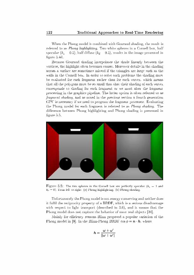
122 Traditional Approa hes to Real-Time RenderingWhen the Phong model is ombined with Gouraud shading, the result isreferred to as Phong highlighting. Two white spheres in a Cornell box, halfspe ular (ks = 0:5), half di�use (kd = 0:5), results in the image presented in�gure 5.4d.Be ause Gouraud shading interpolates the shade linearly between theverti es, the highlight often be omes oarse. Moreover details in the shadinga ross a surfa e are sometimes missed if the triangles are large su h as thewalls in the Cornell box. In order to solve su h problems the shading mustbe evaluated for ea h fragment rather than for ea h vertex, whi h meansthat all the polygons must be so small that that their shading of ea h vertex orresponds to shading for ea h fragment or we must alter the fragmentpro essing in the graphi s pipeline. The latter option is often referred to asfragment shading, and as noted in the previous se tion a fourth generationGPU is ne essary if we need to program the fragment pro essor. Evaluatingthe Phong model for ea h fragment is referred to as Phong shading. Thedi�eren e between Phong highlighting and Phong shading is presented in�gure 5.5.

Figure 5.5: The two spheres in the Cornell box are perfe tly spe ular (ks = 1 andkd = 0). From left to right: (a) Phong highlighting. (b) Phong shading.Unfortunately the Phong model is not energy onserving and neither doesit ful�l the re ipro ity property of a BRDF, whi h is a serious disadvantagewith respe t to light transport (des ribed in 3.6), and it means that thePhong model does not apture the behavior of most real obje ts [30℄.Mainly for e� ien y reasons Blinn proposed a popular variation of thePhong model in [9℄. In the Blinn-Phong BRDF os� = n � h, whereh = ! +!0k! +!0k

5.3 Texture Mapping 123is the half-ve tor between the dire tion to the viewer ! and the dire tion tothe light sour e !0.A modi�ed version of the Blinn-Phong model, in fa t, preserves the ne -essary properties of a BRDF. The modi�ed Blinn-Phong BRDF is given as:fr(x;!;!0) = ks(n � h)m + kdThe relationship between the Phong model and its Blinn-Phong variantwas found in [37℄ as (n � !s)m � (n � h)4m.Sin e all the models des ribed in this se tion only deal with lo al illu-mination, they only simulate the light paths LDE, in ase of the polyhedralmodel, or L(SjD)E, in ase of Phong or Blinn-Phong. To ompensate forthe missing indire t light an ambient term, La, whi h is merely a material onstant, is often added to the shade of an obje t.All these lighting and shading models were kept primitive and simpleto make sure that they would be useful for real-time rendering, and todaythey still are. The Blinn-Phong model ombined with the Gouraud shading(also referred to as Phong highlighting) is the de fa to standard in real-timegraphi s libraries su h as OpenGL. Many expansions seeking to obtain amore physi ally orre t lighting and shading in real-time have been proposedsin e the Phong model, this is the subje t of hapter 6.In the following se tion we will take a brief look at texturing, sin e it isan important part of real-time rendering and be ause textures are useful formany other things than `gluing' pi tures on 3D obje ts.5.3 Texture MappingTextures are used frequently in almost any kind of professional real-time ap-pli ation. They are a heap way to enhan e a Phong highlighted or Phongshaded s ene so that it be ome more visually interesting. Textures often givea s ene the �nal tou h of realism, they are able to add details that wouldotherwise take an immense amount of triangles to render. In ontrast toglobal illumination te hniques (su h as those des ribed in hapter 4), tex-ture mapping an be �grafted onto a standard [real-time℄ rendering methodwithout adding too mu h to the pro essing ost� [134, p. 215℄.Previously we have mentioned that texture mapping as a way to `glue'images on 3D obje ts, and that is indeed the most ommon fun tionalityof textures. The image is usually two-dimensional and we must make it�t the surfa e of a 3D obje t. Points on the surfa e of an obje t an bedes ribed in two dimensions if they are given in parameter spa e oordinates,more ommonly alled (u; v)- oordinates. The texture image is pla ed in theparameter subspa e [0; 1[�[0; 1[. The (u; v)- oordinates are usually providedat the appli ation stage of the rendering pipeline. Graphi s librariries (eg.OpenGL) usually also provide automati texture oordinate generation. The

124 Traditional Approa hes to Real-Time Renderingpro ess of �nding parameter spa e values from lo ations in spa e is alledmapping, hen e the name texture mapping.For a texture to be applied to an obje t, (u; v)- oordinates should beatta hed to ea h vertex of the obje t spe ifying the part of the texture thatought to be drawn at surfa e lo ation on the obje t. Unfortunately it isquite di� ult to over an arbitrary surfa e leanly with a two-dimensionalimage. The texture will most likely be stret hed or ompressed in pla esto �t the surfa e [2℄. A number of options are therefore given before a tex-ture is applied. First we must hoose how to handle the ase where the(u; v)- oordinates rea h outside the texture image de�ned in [0; 1[�[0; 1[.The following options are usually available: Repeat, mirror, lamp to edge,and lamp to border. The di�eren e between lamp to edge and lamp toborder is that in the �rst ase the edge of the texture is repeated when(u; v)- oordinates rea h outside [0; 1[�[0; 1[, while in the se ond ase a sepa-rate border olor an be de�ned, whi h is used for (u; v)- oordinates outside[0; 1[�[0; 1[.The next thing to worry about is whether the texture �t the numberof pixels that the obje t overs on the s reen. The number of pixels thatan obje t overs an hange signi� antly during the ourse of a real-timeappli ation. If the obje t is su� iently lose to the amera it may �ll out allthe pixels on the s reen, while it may also be so far away that it overs a singlepixel only. The �rst ase is alled magni� ation, the se ond is mini� ation.Two �ltering methods are usually available in the ase of magni� ation.Those are nearest neighbor (or a box �lter) and bilinear interpolation. Other�lters ould be used as well. Corresponding �lters are available for mini-� ation. Anyhow mini� ation seems to ause more aliasing problems thanmagni� ation, and it is, therefore, often useful to have a mipmap for mini�- ation.Mipmaps were �rst introdu ed by Lan e Williams in [140℄. Mip is ana ronym from the latin phrase �Multum In Parvo� meaning �many things ina small pla e�. A mipmap is a pyramidal data stru ture where the originaltexture image is the base of the pyramid (level 0). Averaging ea h 2�2 areaof the image into a new texel2 value reates the next level up. This pro ess ontinues until the top of the pyramid ontains only one texel (it is assumedthat the dimensions of the base image are ea h a power of two). Now anappropriate level of the mipmap an be hosen to represent the texture inthe ase of mini� ation.The presentation of texture mapping provided in this se tion has beenvery super� ial. The reason is that many things done with textures mostly on ern anti-aliasing after the image has been stu k on an obje t, and atthe beginning of this proje t we hose not to work on anti-aliasing in detail.2Texel is short for texture element. A texel in a texture orresponds to a pixel on as reen.

5.3 Texture Mapping 125Moreover the ideas that we present in part III do not rely on textures to bestu k on obje ts, rather they use textures as ontainers for data that we �nduseful in a fragment program.The purpose of this hapter was to provide a very basi introdu tion tothe traditional real-time rendering approa h. The rendering method is alledrasterization and it is, in fa t, older than both ray tra ing and radiosity. Wehave presented it here in its modern form, and des ribed the di�erent stagesof the rendering pipeline. The parts of the otherwise hardware implementedpipeline that have been made programmable, have been pointed out. Thenext hapter des ribes some of the methods that are used to expand therasterization approa h in order to push real-time rendering loser to realisti image synthesis. These methods often depend on texture mapping, rasteroperations and the programmable parts of the pipeline (vertex and fragmentprograms).

126 Traditional Approa hes to Real-Time Rendering

Chapter 6Approximating the RenderingEquation in Real-Time

The loser you get to your goal, the harder it will be to rea h it -in fa t, you may NEVER rea h it.Paige Waehner: Exer ise for Beginners - Setting Goals

128 Approximating the Rendering Equation in Real-TimeOne obje tive in this proje t is to approximate, in real-time, as many aspossible of the visual e�e ts that result from a global illumination model.This is not a new obje tive, many resear hers have worked on it before.Many unning methods and lever algorithms have been developed over theyears. Still, not all visual e�e ts are available in real-time, at least notsimultaneously and ertainly not with the same a ura y as if one of themethods for realisti image synthesis had been used.To solve the re ursive integral of global illumination in real-time (havingat most 65 millise onds to spend for ea h image) we must either simplifythe al ulations signi� antly, or otherwise ome up with a simple alternativethat visually gives the same result (we may legitimately all this approa h` heating'). Some of the methods presented in the literature for real-timeapproximation of global illumination are des ribed in this hapter. We willemphasize on the methods that in some way relate to our idea of dire t ra-dian e mapping (see hap. 12), and on methods that an easily be ombinedwith dire t radian e mapping in order to ompensate for the parts of therendering equation that it does not solve.Most arti les addressing the subje t of this hapter fo us on one or asmaller group of visual e�e ts rather than full global illumination. The reasonis that one e�e t alone often is so expensive that it puts heavy restri tionson the resour es left for other methods.The se tions of this hapter are divided into di�erent methods. Se tions6.1, 6.2, and 6.3 des ribe those methods that we ombine with dire t radi-an e mapping in the real-time renderer of this proje t, they are des ribedsu� iently for implementation.A few methods that ould advantageously be ombined with our methodare presented in se tions 6.4 and 6.5. There has not been time for theirimplementation in this proje t, and, hen e, they are not des ribed in detail.We merely bring the readers attention to the appli abilities of these methods.The remaining se tions (6.6, 6.7, 6.8, and 6.9) are methods des ribedfor omparison with dire t radian e mapping. Those methods an not bedire tly ombined with our method, rather they ould ea h repla e it orsome of their on eptual ideas ould be used in ombination with dire tradian e mapping. We an think of them as ompetitors to the dire t ra-dian e mapping method. Therefore we will rather fo us on advantages anddisadvantages of these methods than on their theoreti al foundation.A des ription of di�erent methods for subsurfa e s attering was given inse tion 3.4. This subje t is not addressed any further in this hapter.6.1 Sten iled Shadow VolumesConsider the orre tness of the images in �gures 5.4 and 5.5. One thing wequi kly noti e to be wrong, is that there are no shadows below the spheres.

6.1 Sten iled Shadow Volumes 129The reason is that the shade of ea h vertex (and fragment) is al ulatedlo ally, meaning that other geometry su h as o luding obje ts are not on-sidered when the shade is found.Looking at the derivation of the polyhedral shading model, the simplify-ing assumption that loose the shadows is that of lo al illumination. We ansplit this assumption in two: Dire t illumination only and mutual visibility.The assumption of only dire t illumination has the following result on there�e ted radian e.Lr(x;!) = Z fr(x;!;!0)Li(x;!0) os � d!0= Ze fr(x;!;!0)Li(x;!0) os � d!0where e denotes the dire tions over the hemisphere in whi h a light sour eis visible. If we onsider area light sour es, and use the area formulation ofthe rendering equation instead of the hemispheri al formulation the re�e tedradian e term is given as follows:Lr(x;!) = ZAe fr(x;!;!0)Li(x;!0)V (x;y)G(x;y) dAy= ZA fr(x;!;!0)Le(y;�!0)V (x;y)G(x;y) dAyhere Ae is the surfa e area of all light sour es in the s ene and A is the unionof all surfa e areas in the s ene.The last part of the lo al illumination assumption is mutual visibilitybetween all surfa es, whi h means that V (x;y) = 1 for all x and y. Real-time shadow algorithms seek to avoid this simplifying assumption of mutualvisibility. This se tion presents a fairly general shadow algorithm alledsten iled shadow volumes.The original shadow volume method, presented by Franklin Crow in [22℄,assumes a single light sour e being either a point light or a dire tional light.Dire tional light is a light sour e removed in�nitely far away, whi h results inlight oming from one dire tion only throughout the s ene. In the ase of apoint light pla ed at y, the rendering equation is only slightly more omplexthan the polyhedral model:Lo(x;!) = fr(x;!;!y)V (x;y)Le;0 (n � !y)where n is the surfa e normal at x and !y is the dire tion from x towardsthe light sour e pla ed at y.In ase of a dire tional light the rendering equation is given as follows:

130 Approximating the Rendering Equation in Real-TimeLo(x;!) = fr(x;!;!0)V (x;!0)Le;0 (n � !y)where !0 = �!light, if !light is the dire tion of the dire tional light.The idea proposed by Crow is to let the polygons fa ing the light sour eand their ontour edges extruded away from the light sour e de�ne theshadow volume of an obje t. Surfa es ontained within the volume will be inshadow, while those outside are not. The shadow volume is itself invisible,however, if we draw the shadow volume ea h front fa ing shadow polygonwill tell that everything behind is in shadow, while a ba k fa ing polygonwill an el the e�e t of a front fa ing one.Crow's des ription of shadow volumes (1977) did not �nd a real-timeimplementation until 14 years later in [49℄. The reason being the di� ultiesin drawing an invisible shadow volume, whi h still would be able to spe ifywhether a pixel was in shadow or not. The problem was solved with theemergen e of a sten il bu�er.As des ribed in se tion 5.1 the sten il bu�er stores an integer for ea hpixel in the window. It is possible to use di�erent kinds of masks and sten ilfun tions in order to spe ify the values to be stored in the bu�er.Suppose we have a shadow volume for ea h obje t, then the sten iledshadow volumes algorithm is given as follows:1. Clear the olor, depth, and sten il bu�ers.2. Enable writes to the olor and depth bu�ers. Set the depth test toenable drawing when the depth value is less than the previous value.3. Draw the s ene with ambient lighting only.4. Disable writes to the olor and depth bu�ers. Enable writes to thesten il bu�er.5. Draw the front fa ing shadow polygons. In rement when the depthtest passes.6. Draw the ba k fa ing shadow polygons. De rement when the depthtest passes.7. Disable writes to the sten il bu�er. Enable writes to the olor bu�er.8. Set the sten il test to enable drawing when the sten il value equalszero. Set the depth test to enable drawing when the depth value isequal to the previous value.9. Draw the s ene in full illumination.

6.1 Sten iled Shadow Volumes 131Note how the sten il bu�er �rst ounts how many times a shadow volumeis entered (5.) and afterwards ounts how many times a volume is left behind(6.). If the result of the ount is greater than zero, the surfa e area we arelooking at must still be in shadow, while if the sten il value is zero after the ount has �nished the surfa e area must be free of shadow.The algorithm an easily be expanded to a ount for several light sour es:1. Clear the olor and depth bu�ers.2. Enable writes to the olor and depth bu�ers. Set the depth test toenable drawing when the depth value is less than the previous value.3. Draw the s ene with ambient lighting only.4. For ea h light l:(a) Enable writes to the sten il bu�er. Clear the sten il bu�er.(b) Disable writes to the olor and depth bu�ers. Set the depth testto enable drawing when the depth value is less than the previousvalue.( ) Draw the front fa ing shadow polygons. In rement when thedepth test passes.(d) Draw the ba k fa ing shadow polygons. De rement when thedepth test passes.(e) Disable writes to the sten il bu�er. Enable writes to the olorbu�er.(f) Set the sten il test to enable drawing when the sten il value equalszero. Set the depth test to enable drawing when the depth valueis equal to the previous value. Enable additive blending.(g) Draw the s ene illuminated by light sour e l only.In the above we assume that shadow volumes are available. Though itis quite simple to extrude silhouette edges away from the light sour e toobtain shadow volumes, it is also quite expensive. One relatively e� ientway, presented in [2, 12℄, is to draw ea h edge as a quadrilateral (or quad) ofno width. Two polygons meet where ea h edge quad is drawn, two verti esof the quad should have normals from one polygon and two verti es shouldhave normals from the other polygon. When drawing the shadow polygonsto the sten il bu�er, a vertex program an move verti es away from the lightsour e if their normal points away from the dire tion towards the light. Thisapproa h will extrude silhouette edges for shadow volumes.Compared to other shadow algorithms sten iled shadow volumes are,as mentioned, fairly general. Some shadow algorithms, su h as proje tionshadows, an only ast shadows on planar surfa es. For some algorithms,

132 Approximating the Rendering Equation in Real-Timeeg. shadow textures, it is ne essary to spe ify whi h obje ts that are o lud-ers and whi h obje ts that are re eivers. An alternative to shadow volumesis shadow maps introdu ed by Lan e Williams in [139℄. In short the shadowmap is a pi ture from the light sour e and everything that is not seen in thismap is in shadow. The shadow map an, as shadow volumes, ast shadowsfrom arbitrary geometry onto arbitrary geometry. There are di�erent prob-lems asso iated with ea h method. The shadow map mostly su�ers fromaliasing problems, while shadow volumes su�er from problems of a more ge-ometri al nature. Most of the problems in shadow volumes are addressed in[78, 34℄ and we will not go further into them at this point.The limitations of shadow volumes are still the simplifying assumptionsof only dire t illumination and only point or dire tional light sour es. The�rst assumption is fundamental to all shadow algorithms. In order to removethis assumption we must al ulate the mutual visibility between all surfa elo ations in a s ene, whi h is quite infeasible for a shadow algorithm that inits simple form annot simulate light sour es with an areal extension. Thelatter assumption has been addressed lately by several arti les. The pointand dire tional light sour es result in hard shadow edges, sin e they haveno areal extension that an make a sour e partly visible. The visual e�e tresulting from area light sour es is known as soft shadows.The extension that makes the sten iled shadow volumes algorithm able tosimulate soft shadows, is not straight forward. One method, des ribed in [51℄,uses an extended shadow map alled a D-bu�er to store umbra and penumbravolumes1. Another approa h, presented in [7, 8, 1℄, al ulates penumbrawedges and use them for approximation of soft shadows. Unfortunately wehave not had time for an implementation of real-time soft shadows during thisproje t. A good presentation of shadow volumes and the penumbra wedgesextension is given in [35℄. A general overview of the di�erent algorithms anbe found in [2℄.This se tion on erned the dire t illumination approximation of the ren-dering equation. Dire t illumination in lude shadows and it is, therefore,better than the lo al illumination models presented in se tion 5.2. The nextstep towards visual realism is spe ular re�e tions, whi h is the subje t of thetwo following se tions.6.2 Planar Re�e tions Using the Sten il Bu�erRe all from se tion 4.4 how the rendering equation an be split up into fourdi�erent terms: Dire t illumination, spe ular and glossy re�e tions, austi s,and multiple di�use re�e tions. Having dire t illumination, the next steptowards global illumination is to simulate spe ular re�e tions. To start out1Umbra denotes an area in full shadow. Penumbra denotes an area partly in shadow.

6.2 Planar Re�e tions Using the Sten il Bu�er 133simple, we �rst onsider single spe ular re�e tions for planar surfa es (lightpaths LD?SpE, where Sp denotes spe ular re�e tions o� planar surfa es only).In global illumination spe ular re�e tion is an e�e t available throughray tra ing. This se tion will introdu e a rasterization approa h to spe ularre�e tion, making it available in real time.As des ribed se tion 3.1 the angle of re�e tion equals the angle of in i-den e. In ase of a planar re�e tor, the re�e tion of a s ene is in other wordsan inversion of the s ene in the plane representing the re�e tion surfa e.Figure 6.1 illustrates how the re�e tion an be represented as a rendering ofthe s ene from an inverted virtual viewpoint.

Reflecting plane

Eye point e

Reflected eye point er

Scene

Reflected Scene

d

i

r

n

Figure 6.1: A s ene re�e ted in a plane (planar re�e tion). The re�e tion an be seenas a re�e tion of the s ene geometry in the re�e ting plane or as a rendering of the s enefrom a re�e ted eye point. This �gure is a reprodu tion of �gure 6.1 in [90℄.The position and viewing dire tion of the re�e ted eye point er and there�e ted viewing dire tion r an be found from the position of the originaleye point e and the original viewing dire tion i, using the following twoformulas: er = e+ 2d(�n)r = i� 2(n � i)nwhere n must be a unit surfa e normal of the planar re�e tor. Here r isfound using (3.2). Note, however, that signs have been hanged sin e ipoints towards the surfa e not away from it.One way to implement planar re�e tions is simply to render the s enefrom the re�e ted eye point in the re�e ted viewing dire tion. Afterwards

134 Approximating the Rendering Equation in Real-Timethe result is shown in the re�e ting surfa e.Another method, whi h is used more frequently, makes use of the sten ilbu�er. This is also the method implemented for this proje t. The generalidea is to let the sten il bu�er lip out the part of a s ene that should bere�e tive and then render the re�e ted s ene in this area of the s reen. Byuse of the sten il bu�er we will only need to render the visible part of there�e ted s ene instead of the entire re�e ted s ene. An example of how this an be done is to render the s ene in one pass and sten il mark the pixels ofthe re�e ting obje t. Then render the re�e ted s ene into the marked areain the se ond pass [90℄.The step by step algorithm of planar re�e tion using the sten il bu�erappears in [70℄ as follows:1. Clear the olor, depth, and sten il bu�ers.2. Enable writes to the olor and depth bu�ers. Disable writes to thesten il bu�er.3. Render the s ene ex luding re�e ting surfa es.4. For ea h re�e ting surfa e:(a) Disable writes to the olor bu�er. Set up sten iling to write thevalue 1 into the sten il bu�er when the depth test passes.(b) Draw the polygons of the re�e ting surfa e. Thereby all planarre�e tors that are not o luded will be `tagged' in the sten ilbu�er.( ) While the olor bu�er is still disabled, set the depth range towrite the farthest value possible for all updated pixels and set thedepth test to always pass. Also, set the sten il test to only updatepixels tagged with the sten il value 1.(d) Draw the polygons of the planar re�e tor on e again. This will lear the depth bu�er for all visible pixels of the planar re�e tor.(e) Reset the depth test and the depth range. Re-enable the olorbu�er.(f) Establish a lip plane to render obje ts on the re�e tive side ofthe mirror plane only.(g) While still only updating pixels marked in the sten il bu�er, ren-der the s ene mirrored in the plane of the re�e ting surfa e.The sten il bu�er marks the area in whi h re�e tions o ur in the s ene,in this way only the re�e tive part needs to be onsidered when al ulatingthe re�e ting image. This prevents unne essary al ulations. The sten iled

6.3 Cube Environment Mapping 135planar re�e tions have been implemented for our demonstration appli ationdes ribed in part III.Planar re�e tions an also be simulated using texture mapping. Thispro edure is straight forward and uses two passes. First pass renders there�e ted s ene into a texture and se ond pass maps it to the re�e ting obje t[79℄.An advantage of using the sten il bu�er pro edure is that we will onlyneed to update the pixels of the re�e ting obje t. When using texture map-ping, we an have problems with magni� ation and mini� ation artifa ts ifthe eye point is too lose or too far away [90℄. These artifa ts will not appearin the sten il bu�er method, sin e the s ene is a tually rendered.If two re�e tive surfa es are fa ing ea h other re�e tions inside the re-�e tions should be generated. In prin iple this re�e tion should go on forever. A re�e tion loop like this is referred to as re ursive re�e tions, whi h an be rendered using real time approa hes as well. The planar re�e tionalgorithm is re ursively repeated a number of times. This number dependson the max re ursion depth that is a parameter for how many re�e tions in-side re�e tions there should appear. The pro edure is des ribed in [90, 91℄.Meaning that we an simulate the light paths LD?Sp*E using this approa hand dire t illumination, whi h brings us even loser to a full implementationof the spe ular term in real-time. The following se tion further explores thisopportunity by des ribing a method for simulation of spe ular re�e tions on urved surfa es.6.3 Cube Environment MappingIn order to have a better approximation of the rendering equation, we mustbe able to a ount for spe ular re�e tions on urved surfa es as well as onplanar surfa es. Unfortunately the te hnique for urved surfa es is not wellsuited for planar surfa es and vi e versa, therefore we need both approa hes.The light paths we wish to simulate in this se tion are LD?S E, and we aneven expand this approa h to in lude multiple spe ular re�e tion (light pathsLD?S +E).Environment mapping was introdu ed in 1976 by Blinn and Newell in[10℄. It is a way to make urved obje ts appear to re�e t the surroundingsbased on images saved in textures. The on ept is to reate an environmentmap des ribing the surroundings of the re�e tive obje t. The re�e tion isthen simulated through lookups in the map. Environment mapping hasbe ome one of the most popular methods for generating perfe tly spe ularre�e tions in real time.Environment mapping has ertain limitations. The map is reated from asingle point in spa e (usually the enter point of the re�e tive obje t), mean-ing that the geometry of the re�e tion is only a urate if the surfa e point

136 Approximating the Rendering Equation in Real-Timeis at the obje t enter or if the re�e ted environment is in�nitely distant.This means that all the surroundings, in fa t, are re�e ted at the enter ofthe re�e ting obje t. In pra ti e it means that obje ts lo ated lose to there�e ting surfa e will be re�e ted in orre tly, if the obje t lose by is large,the e�e t will not be parti ularly noti eable. Shadows re�e ted on surfa es lose to the re�e tor seem to ause the biggest problems. Another limitationto environment mapping is that the re�e ting obje t not will be re�e ted initself.Di�erent environment mapping methods exists. Sphere mapping, ubemapping, and dual paraboloid mapping are all supported dire tly by graphi APIs and graphi s a elerators. Good des riptions of these an be foundin [90℄. In this proje t we have used ube environment mapping, whi htherefore will be the only one that we des ribe. The main prin iples of ubeenvironment mapping will now be presented.Creating an environment map is like drawing the surroundings of a re-�e ting obje t to a texture. The approa h for environment ube mapping isto �nd a map for ea h of the six sides of a ube surrounding the re�e ting ob-je t. The resulting texture maps pi ture the parts of the surroundings thatare visible from the enter of the re�e tive obje t in all dire tions. Figure6.2 shows the on ept of the environment ube map.The ube environment map is view independent; if the eye point hangesposition only re al ulation of the re�e tion ve tors is needed to provide the orre t re�e tion. The texture must be re- al ulated though if the surround-ings or the position of the re�e tor hange.In order to re�e t a s ene dynami ally we must generate the textures forthe environment ea h frame. The following steps are ne essary in order torender the environment dynami ally [142℄:1. Set up a amera with a 90Æ �eld of view at the enter of the re�e tingobje t's lo ation.2. Point the amera along +x and render the (approximate) s ene aroundyour obje t into the �rst fa e of the ube map.3. Repeat the pro ess, rendering along �x, �y and �z into ea h fa e ofthe ube map.When rendering the ube map the re�e ted dire tion (r) of ea h fragmentis used as texture oordinates for the look-up in the environment map. We an also reate a single level of refra tion if we use the refra ted dire tion astexture oordinates.In luding multiple spe ular re�e tions in this approa h is surprisinglysimple and inexpensive with respe t to pro essing time. We merely in ludethe environment maps found in the previous frame, when rendering otherspe ular obje ts in the images for the di�erent fa es of the environment

6.3 Cube Environment Mapping 137

-x +x

-y

+y

+z

-z

Folded

Front Left Right

Top

Bottom

Back

Unfolded

+z

+y

+x

-z

+x

+y

+x

+z

-z

+y

-x

+y

Figure 6.2: The on ept of environment mapping. Ea h side of the ube is renderedand stored in a texture. The ube sides are referred to as ube fa es.map. This e�e tively provides an extra spe ular re ursion for ea h framethat we render without mu h extra e�ort.Adding the light paths that we an simulate using environment mappingto the light paths we an simulate using sten iled planar re�e tions (see theprevious se tion), it is all in all possible to approximate a spe ular termusing real-time rendering methods. The limitation is that we �nd re�e tionso� perfe tly spe ular materials only. This an be ompensated for by use ofblending, sin e the glossy e�e ts that should be simulated by the spe ularre�e tions term of the rendering equation only in lude those glossy surfa eswe have lassi�ed as loser to spe ular obje ts than di�use obje ts.

138 Approximating the Rendering Equation in Real-TimeThe spe ular term found simulate the light paths LD?S+E. If we let dire tillumination simulate LD?E, the resulting rendering method will simulate thepaths LD?S*E. The spe ular term found here is not entirely omparable to thespe ular and glossy re�e tions term des ribed in photon mapping ( f. se .4.4), whi h simulate the paths LS*(S|D)S+E. The missing part is re�e tionof austi s, whi h we annot a omplish unless we employ a method that ansimulate austi s in the �rst pla e. In the following se tion we will dis uss afew methods that ould be used to simulate austi s in real-time.6.4 Real-Time Causti sThough there has not been time for a real-time implementation of austi sduring this proje t, we would like to point out some of the methods thathave been presented in literature, sin e they an be used in ombinationwith the methods mentioned previously in this hapter and with our ownmethod alled dire t radian e mapping as well.The only rasterization approa h to real-time austi s that we are awareof is presented in [130℄. The idea is to �dis retize the surfa e of a spe ularre�e tor into small regions and treat ea h as a pinhole amera that proje tsthe in oming light onto the surrounding obje ts�. Unfortunately the ap-proa h is prone to aliasing artifa ts and the results are not too onvin ing.Nevertheless it is one possible way to render austi s in real-time.All other approa hes to real-time austi s that we have ome a ross seekto simulate photon mapping in real-time. Even if some approa hes simulatethe entire photon mapping algorithm, the austi s an (as shown previously)be separated from the rest of the photon mapping method and used individ-ually in ombination with other methods.Pur ell et al. [108℄ des ribe how photon mapping an be implementedin graphi s hardware. They use a �ltered dire t evaluation of a global pho-ton map whi h result in visible low frequen y noise with respe t to indire tillumination. Their pro essing times are unfortunately measured in se ondsper frame (not fps). Donner and Jensen [28℄ have subsequently des ribedhow the pro essing time of the GPU omputations an be improved usingadaptive re�nement. Using the method for austi s alone and ombining itwith other methods for the remaining omputations, would probably resultin better frame rates.Real-time austi s an be a hieved using distributed photon mapping.Günther et al. [44℄ show how austi s an be rendered using a luster of9 to 36 CPUs. This is, however, less interesting with respe t to real-timerendering on a single CPU, whi h is the obje tive of this proje t. On theother hand they also present some interesting optimizations for photon map-ping on a single ma hine. For example they use a variant of sele tive photonemission, whi h was originally introdu ed in [27℄, and they use alternative

6.5 Complex BRDFs 139data stru tures for storage of the photon map, see se tion 2.5.Finally an interesting method for simulation of photon mapping in real-time is presented by Larsen and Christensen in [74℄. The method is alsodes ribed in se tion 6.7, but pi k out the austi s method for now. The austi s al ulations use a pbu�er2 to ount the number of austi photonsending up in ea h fragment. Using this pbu�er as a texture for a fragmentprogram, makes the fragment program able to determine the ontribution ofthe austi s term in ea h fragment. A simple �lter is applied whi h takesthe austi s term of nearby pixels into a ount. The results are promisingand the implementation is quite straight forward, even though an e� ientray tra er is needed for photon tra ing.In the following se tion, we will des ribe a few omplex BRDFs that anenhan e the shading methods normally used for real-time appli ations.6.5 Complex BRDFsEven the modi�ed Blinn-Phong BRDF (see se . 5.2) is not very lose to aphysi ally orre t BRDF. The emergen e of programmable graphi s hard-ware has given a good opportunity for implementation of more omplexBRDFs in real-time shading. In this se tion we shortly present a physi allybased BRDF and an empiri al BRDF.The Cook-Torran e ModelThe Cook-Torran e BRDF is a physi ally based model, and it is a signi�- ant improvement ompared to the modi�ed Blinn-Phong model. It is quiteexpensive though. The math is given as follows [21℄:fr(x;!;!0) = F (�)� D(�h)G(n � !)(n � !0) + kd (6.1)where os � = h � ! = h � !0 and os �h = n � h. h is the half-ve tor.D simulates mi ro-fa ets for the material and is given as:D(�h) = 1�2 os4 �h e�(tan �h=�)2where � is a material parameter (it might be referred to as a measure ofroughness).G aptures masking and self-shadowing by the mi ro-fa ets:G = min�1; 2(n � h)(n � !0)!0 � h ; 2(n � h)(n � !)!0 � h �2pbu�er is short for pixel bu�er and it is an o� s reen bu�er for storing rendered imageswhi h need not appear on the s reen.

140 Approximating the Rendering Equation in Real-TimeThe Ward ModelThe Ward model is an empiri al model, meaning that it primarily intends to�t experimental data. It is less expensive than Cook-Torran e and it in ludesan intuitive set of material parameters: �d, the di�use re�e tan e, �s, thespe ular re�e tan e, and �, the surfa e roughness. The BRDF is given asfollows [132℄: fr(x;!;!0) = �d� + �s e�(tan �h=�)24��2p(n � !)(n � !0) (6.2)as before os �h = n � h and h is the half-ve tor.This on ludes the se tions on erning methods that an be ombinedwith dire t radian e mapping. In the following we will des ribe ompetingmethods, whi h all seek to evaluate the multiple di�use re�e tions term.First we will look at a traditional te hnique for real-time `pseudo-global'illumination alled light mapping.6.6 Light MappingOne obvious advantage of radiosity ompared to other global illuminationte hniques is that it omputes lighting throughout the s ene, and that thislighting is stati as long as the obje ts do not move. The reason is theassumptions of di�use surfa es only. Di�use surfa es re�e t light equally inall dire tions over the hemisphere, and the resulting view-independen e hasthe e�e t that the ontribution of light to a surfa e an be aptured in atexture and atta hed to the surfa e.The on ept of lighting information atta hed to a surfa e using a textureis referred to as light mapping. After the light maps have been reatedthey an be used for real-time rendering nearly without expenses. In di�useenvironments it will even be di� ult to noti e that the lighting does not hange a ordingly when obje ts are moved around. The illusion, however,qui kly breaks if we start moving the light sour e around, or if we pla e ablue ball in front of the light sour e and noti e that the olor bleeding doesnot hange.Still, light mapping is an inexpensive and widely used te hnique whi h an simulate multiple di�use re�e tions in real-time. In [109℄ it is des ribedhow radiosity was al ulated on graphi s hardware and stored in light mapsfor real-time use in a large s ale game from Atari alled �Shadow Ops�.In order to use radiosity stored in light maps in ombination with themethods des ribed previously in this hapter, we must hoose either to in- lude the dire t illumination term in the radiosity al ulation, whi h willresult in obvious �aws when obje ts are moved, sin e the shadows will notmove a ordingly. Alternatively we an adjust the radiosity algorithm to

6.7 Real-Time Photon Mapping Simulation 141make sure that the light maps only in lude light re�e ted di�usely at leaston e. In this way the light map an be ombined with the dire t illuminationterm using blending.Other global illumination te hniques ould be used with light mappingas well as radiosity an. We must always make sure, though, that only themultiple di�use re�e tions term is omputed, if we plan to ombine the lightmapping with other methods. The reason why it is lever to use light mapsonly for the multiple di�use re�e tions term is that the indire t illumination hanges quite slowly over the surfa es and therefore it will be less noti eablethat su h lighting is stati .To summarize light mapping an reate sophisti ated lighting at mini-mum ost for stati s enes illuminated with stati light sour es. An opti-mization of the on ept is to store only light re�e ted di�usely at least on ein the light map, and then ombine the light mapping te hnique with othermethods for di�erent parts of the rendering equation. Still, if we need ourappli ation to simulate dynami indire t lighting, or if we do not have timefor a global illumination prepro essing stage, we have to look for di�erent ap-proa hes to an evaluation of the multiple di�use re�e tions term. A brilliantreferen e for further information on light mapping te hniques is [16℄.The next se tion des ribes real-time simulation of photon mapping, whi hwe also had a brief look at with respe t to real-time austi s in se tion 6.4.6.7 Real-Time Photon Mapping SimulationA unning real-time implementation of photon mapping is presented in[72, 74℄. The part of this implementation that simulates the multiple di�usere�e tions term is, of ourse, a ompetitor to our own method for omputa-tion of the same term. The real-time photon mapping approa h ould equallywell be ombined with the methods des ribed in se tions 6.1 through 6.5.The real-time simulation of photon mapping �rst seek out the di�erentsurfa es in a s ene. A ording to the method des ribed in [73℄, a global pho-ton map is reated for ea h surfa e (this speed up photon map onstru tionand radian e estimates).A variant of the sele tive photon emission des ribed in [27℄, is used toemit only intelligently sele ted photons ea h frame. Using sele tive photonemission, the photons are emitted in groups. The method presented in [74℄emits one photon for ea h frame from ea h group. The path of the previousphoton emitted in ea h group is stored. If the path taken by a photon in agroup is not the same as the previous path, the entire group of photons ismarked for redistribution.For ea h surfa e a texture is generated holding radian e estimates fromthe photon map related to that parti ular surfa e. These textures are re-ferred to as approximated illumination maps.

142 Approximating the Rendering Equation in Real-TimeA hardware optimized �nal gathering method is presented, where a num-ber of lo ations on the surfa es of the s ene are hosen (eg. by the modeler).The approximated illumination maps are applied to ea h surfa e and then api ture is taken from ea h hosen lo ation to simulate �nal gathering rays.The resulting pi tures are averaged using hardware optimized mipmapping(the topmost image in the mipmap is the average). The result is a number ofpre-determined lo ations distributed over the surfa es throughout the s enewhere the multiple di�use re�e tions term is known - we ould all it anindire t illumination �eld.One way to visualize this indire t illumination �eld is simply to store theindire t illumination in oarse textures, whi h an then be applied to thesurfa es where the indire t illumination was al ulated. This approa h isfeasible sin e di�usely re�e ted indire t illumination usually hanges slowlyover a surfa e.Compared to light mapping this method handles dynami s enes illu-minated by dynami light sour es. Furthermore it potentially simulates allkinds of light paths in the multiple di�use re�e tions term (L(SjD)*DS*DS*E).The approximate �nal gathering unfortunately smooth out the result3, butthis is relative sin e it depends on the number of lo ations we hoose onthe di�erent surfa es. The resulting illumination in a Cornell box using thismethod is almost indistinguishable from the global illumination referen e(see [72℄).An additional work load that must be added to an implementation ofthis method is an e� ient ray tra er, whi h must be available for the pho-ton tra ing. E� ient ray tra ing involves spatial data stru tures (eg. BSPtrees) whi h put some restri tions on the s ene geometry. If obje ts are an-imated or if they morph during rendering, the spatial data stru tures mustbe re onstru ted, this pro ess may be quite expensive with respe t to pro- essing time. Also dynami obje ts should be pointed out in advan e andea h of them should have an individual data stru ture, sin e re onstru tionof a global spatial data stru ture ea h frame is too expensive.Another disadvantage is the �nal gathering method where many low res-olution pi tures are taken at pre-determined lo ations in the s ene geometry.This approa h is not easily s aled to large and omplex s enes, the numberof approximated illumination maps that must be pro essed will es alate.We have now des ribed light maps, whi h pre- ompute a stati ase ofglobal illumination and store the result in a texture for ea h surfa e. Besideswe have des ribed a method for dynami simulation of global illuminationin the form of photon mapping. The next se tion will des ribe an approa hthat seeks to take the best of both worlds and ombine pre- omputation with3This is unfortunate sin e smoothing the indire t illumination has the result that only lose to perfe tly di�use surfa es an be handled at this last boun e of di�usely re�e tedindire t illumination.

6.8 Pre- omputed Radian e Transfer 143dynami lighting.6.8 Pre- omputed Radian e TransferIn radiosity form fa tors represent energy transfer between surfa es. It isassumed that all surfa es re�e t light di�usely and that radiosity is onstanta ross the surfa e of a pat h, hen e, we need not onsider the dependen e ondire tion and lo ation. This is why form fa tors represent energy transfer.If we remove the assumption of di�use surfa es only, the on ept of formfa tors an be generalized to represent irradian e transfer (instead of energytransfer) between surfa es. In pra ti e this means that an arbitrary BRDFmust be in luded in the radiosity form fa tor.In [122℄ it is shown how a olle tion of spheri al harmoni s basis fun tions an represent su h generalized form fa tors, or irradian e transfer fun tions.The reason for using spheri al harmoni s is that �a �nite number of terms anbe used to approximate relatively smooth fun tions de�ned on the sphere�[122, p. 192℄.The on ept of pre- omputed radian e transfer, des ribed in [123℄, is tolet a dense set of ve tors or matri es over a surfa e represent its radian etransfer fun tion. The radian e transfer fun tion is a further generalizationof the spheri al harmoni s based approa h des ribed in [122℄. The radian etransfer fun tions are su� iently general to be used for the evaluation of therendering equation dire tly.Though arbitrarily omplex BRDFs an be simulated using radian etransfer fun tions. The pre- omputed radian e transfer methods often limitthemselves to low-frequen y lighting only. The reason is that di�use sur-fa es, and glossy surfa es with di�use hara teristi s, typi ally require fewerspheri al harmoni s basis fun tions in the radian e estimate than spe ularsurfa es do. Fewer basis fun tions means fewer omputations and, hen e, themethod be omes less expensive and less prone to aliasing artifa ts resultingfrom an insu� ient order of the spheri al harmoni s basis.The approa h is then to pre- ompute for a given surfa e the radian etransfer fun tions, whi h are independent of the in ident radian e term. Asummation over inner produ ts between the transfer fun tions and in identradian e samples on a surfa e then gives an inexpensive, dynami , approxi-mate evaluation of the rendering equation.Be ause of extensive pre- omputations the method is restri ted to use ofrigid obje ts only. The `simple' version of pre- omputed radian e transferonly works for radian e transfer from a onvex, rigid obje t onto itself. Thisis alled self-transfer. In [123℄ a method is also des ribed for neighborhood-transfer, where radian e transfer fun tions are also omputed from a rigidbody to its neighbor spa e. This expansion allows soft shadows, glossy re-�e tions, and austi s on dynami re eivers.

144 Approximating the Rendering Equation in Real-TimeThe neighborhood-transfer is important if the method is to be useful in a omplex s ene omposed of many moving obje ts. However, neighborhood-transfer has problems when multiple obje ts re�e t light or ast shadows onthe same re eiver. Moreover the lighting must be fairly onstant a ross theentire neighborhood of an obje t to provide a urate results. This indi atesthat pre- omputed radian e transfer is a brilliant method if only a single(or a few) obje ts are present in a s ene at the same time (a s enario ouldbe a dynami virtual hara ter �lling out the entire s ene while talking tothe user of a 3D appli ation). In more dynami environments the methodunfortunately falls apart. And lastly the developer using the method mustbe prepared for long pre- omputation times.A very di�erent method �nding mu h inspiration in the same ba kgroundas pre- omputed radian e transfer, is the subje t of the next se tion.6.9 Environment Map RenderingAfter it was shown in [122℄ how a spheri al harmoni s representation ould bederived for arbitrary BRDFs, the on ept has subsequently been ombinedwith environment mapping in [110, 111℄. The approa h used here was spheremapping (where the sphere map is a two-dimensional image of a sphere). Thesphere environment map represents the irradian e transfer fun tions used forspheri al harmoni s approximation of an arbitrary BRDF.In a di�erent ontext Greger et al. [43℄ had shown that irradian e volumesspa ed in a regular grid a ross a s ene ould be used for storage and inter-polation of global illumination in a s ene. Irradian e volumes is des ribedas an extended version of irradian e, whi h is de�ned in all points and di-re tions in spa e. This means that irradian e volumes are de oupled froms ene geometry. (In our opinion a better des ription of an irradian e volumeis that it aptures radian e transfer in all dire tions at a ertain point in thes ene.) Irradian e volumes were originally presented for pre- omputationwith traditional global illumination te hniques.A brilliant idea, presented in [77, 93, 92℄, is to ombine the environmentmapping representation of transfer fun tions with the irradian e volumesapproa h to global illumination. Instead of sphere maps, ube environmentmaps are used for storage of radian e transfer fun tions. Those ube mapsare spa ed in a regular grid of 4� 4� 4 a ross the s ene. Ea h environmentmap is updated ea h frame using the same te hnique for environment mapsas des ribed in se tion 6.3.Sin e the transfer fun tions are de oupled from geometry and regularlyspa ed in the s ene, a radian e estimate at an arbitrary lo ation s in thes ene is found by tri-linear interpolation to s from the �irradian e volumes�pla ed at the orners of the grid ells.When mapping this method to the GPU, di�erent spheri al harmoni s

6.9 Environment Map Rendering 145 oe� ients are al ulated using the environment maps and stored in 3D tex-tures whi h are uploaded to the GPU in order to ompute radian e estimatesin a fragment program.Though frame rates are below 10 per se ond, the results of this methodlook promising. Even for rather omplex s enes. A ording to Nijasure et al.there are only few limitations to their te hnique, and they propose solutionsfor all the problems they des ribe. One problem is that the 4 � 4 � 4 griddimension is not su� ient for large s enes. The solution they propose is tospa e the grid non-regularly in the view frustum. This may, however, resultin a new problem, sin e the tri-linear interpolation may be in orre t if thegrid is non-uniform.They also note that their urrent implementation do not support arbi-trary BRDFs, though the method does not ex lude them. We must keep inmind though that spe ular surfa es will be prone to aliasing artifa ts be auseof the general limitations of the spheri al harmoni s approximation, whileglossy surfa es with di�use hara teristi s an be simulated if some extrapro essing time is set o� for the radian e estimate.A third problem about the method is olor or shadow leakage. Someleakage is aused by the tri-linear interpolation s heme. A method that an handle this problem is presented in [92℄, though it an not (yet) beimplemented in hardware.Problems not mentioned, are problems asso iated with the spheri al har-moni s representation of the radian e transfer. A ording to [122℄ and [123℄some aliasing artifa ts an o ur if too few spheri al harmoni s oe� ientsare omputed. Another issue is that spheri al harmoni s are de�ned over theentire sphere and therefore it is di� ult to ompletely remove the radian ein one dire tion from an �irradian e volume� if it is positioned lose to ano luding obje t. This problem an result in light leaking through walls.All that said, the reported results are still quite impressive. This methodwill be hard to ompete against. Let that on lude our des ription of existingmethods for real-time simulation of global illumination.

146 Approximating the Rendering Equation in Real-Time

Part IIModeling Contents

149All of part I is based on the geometri al representation of a s ene and the al ulation of illumination in it. This part will on entrate on the reation ofa s ene and how to alter the s ene in order to reate a dynami appli ation.S enes are normally reated in a modeling program; in this proje t we haveused the modeling program alled Blender, whi h is freeware. In the model-ing program there are settings for light sour es, materials, and amera, andalso animation features for moving things around in the s ene. The termsused for modeling an sometimes be di�erent from those used in the theory,espe ially when it omes to materials and light. During this part we will tryto introdu e some of the typi al terms for light and material settings andrelate them to the theory. Blender will also be shortly introdu ed in thispart.The �rst hapter of this part - hapter 7 - will des ribe how to model 3Ds enes that are omposed of polygons, as these most often are the primitivesused in real-time graphi s. Though obje ts in a s ene are normally reatedfrom polygons, there are several handy methods for reating the `right' poly-gons. Sometimes obje ts are reated from urves or primitives and thentransformed into polygons by the appli ation, we have, however, restri tedourselves in this proje t to a des ription of polygonal modeling only.Just after the obje ts of a s ene have been reated they appear dull,this is until material or textures are applied to them. There are a bun h ofparameters that an be adjusted to make the obje ts look exa tly right, aswell as di�erent spe ial e�e ts that an be used to reate realisti obje ts.Chapter 8 on erns material settings and textures.To make a s ene even more interesting, from a users point of view, wemust make it ome alive, meaning that some obje ts in the s ene shouldmove about. This is the subje t of hapter 9. Obje ts following a seriesof movements over a predetermined number of frames are referred to asanimated obje ts. There are di�eren es between animation for movies andintera tive appli ations su h as games; those will also be dis ussed in hapter9. After going through di�erent aspe ts of modeling we turn to the modelingappli ation. Chapter 10 will introdu e how s enes are reated using Blender.The hapter will introdu e those features that we have used for reation ofour test s enes, and show how those features des ribed in hapters 7, 8, and9 are used in pra ti e. Sin e we want to test our own renderer with thes enes that we reate in Blender, we need to export our s ene. How this isdone will also be explained in hapter 10.

150

Chapter 7Modeling 3D S enes

We do not grow absolutely, hronologi ally. We grow sometimesin one dimension, and not in another; unevenly. We grow par-tially. We are relative. Anaïs Nin

152 Modeling 3D S enesIn this hapter we will give a brief introdu tion to some of the on eptsbehind 3D modeling. As neither of us has any professional angle to modeling,this hapter will not address any advan ed methods, it will rather presentthe knowledge we have a hieved while modeling during this proje t. Wewill onsider polygonal modeling only. Subje ts des ribed in this hapterare presented from a Blender point of view, where Blender is the modelingappli ation used to reate our test s enes.Obje ts in most real time appli ations are built from polygons onne tedin so alled polygon meshes. A polygon mesh an be reated automati allyby the modeling appli ation, from primitive obje ts, extrusions, or polygonsweeps arried out by the user, or they an be reated one polygon at thetime.One simple way to reate polygon meshes is by use of primitive obje ts.The primitive obje ts available in Blender are presented in �gure 7.1. Forexample we an reate a primitive person from a ube, a sphere and four ylinders, see �gure 7.2.

Figure 7.1: The primitives available in Blender. Top left to bottom right: A plane, atube, and a box. A sphere, a ylinder, and a one.The shape of the primitives, whi h the person is omposed of, have hanged a little ompared to those in �gure 7.1. The ube is now �attenedand the ylinders are stret hed and slimmed to �t the shape of body, arms,

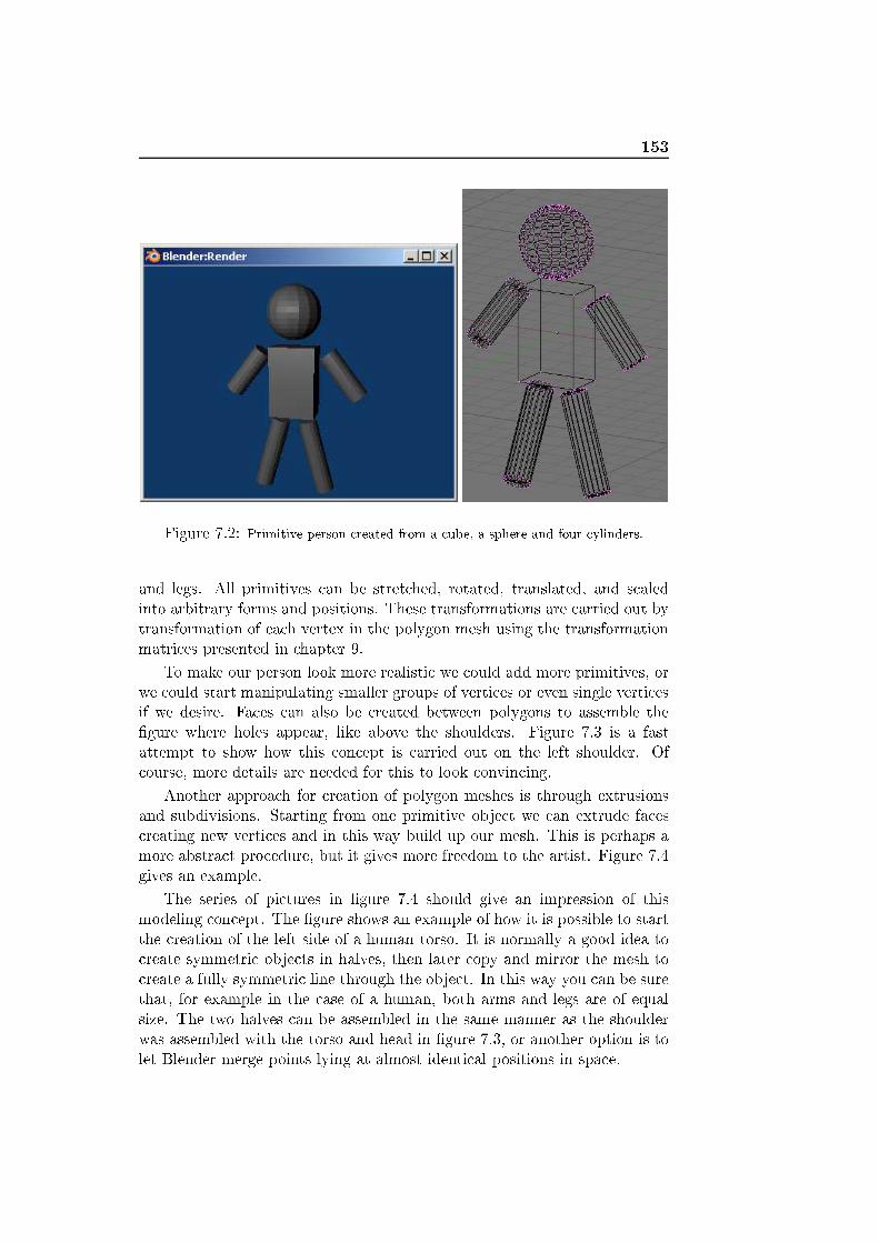
153

Figure 7.2: Primitive person reated from a ube, a sphere and four ylinders.and legs. All primitives an be stret hed, rotated, translated, and s aledinto arbitrary forms and positions. These transformations are arried out bytransformation of ea h vertex in the polygon mesh using the transformationmatri es presented in hapter 9.To make our person look more realisti we ould add more primitives, orwe ould start manipulating smaller groups of verti es or even single verti esif we desire. Fa es an also be reated between polygons to assemble the�gure where holes appear, like above the shoulders. Figure 7.3 is a fastattempt to show how this on ept is arried out on the left shoulder. Of ourse, more details are needed for this to look onvin ing.Another approa h for reation of polygon meshes is through extrusionsand subdivisions. Starting from one primitive obje t we an extrude fa es reating new verti es and in this way build up our mesh. This is perhaps amore abstra t pro edure, but it gives more freedom to the artist. Figure 7.4gives an example.The series of pi tures in �gure 7.4 should give an impression of thismodeling on ept. The �gure shows an example of how it is possible to startthe reation of the left side of a human torso. It is normally a good idea to reate symmetri obje ts in halves, then later opy and mirror the mesh to reate a fully symmetri line through the obje t. In this way you an be surethat, for example in the ase of a human, both arms and legs are of equalsize. The two halves an be assembled in the same manner as the shoulderwas assembled with the torso and head in �gure 7.3, or another option is tolet Blender merge points lying at almost identi al positions in spa e.

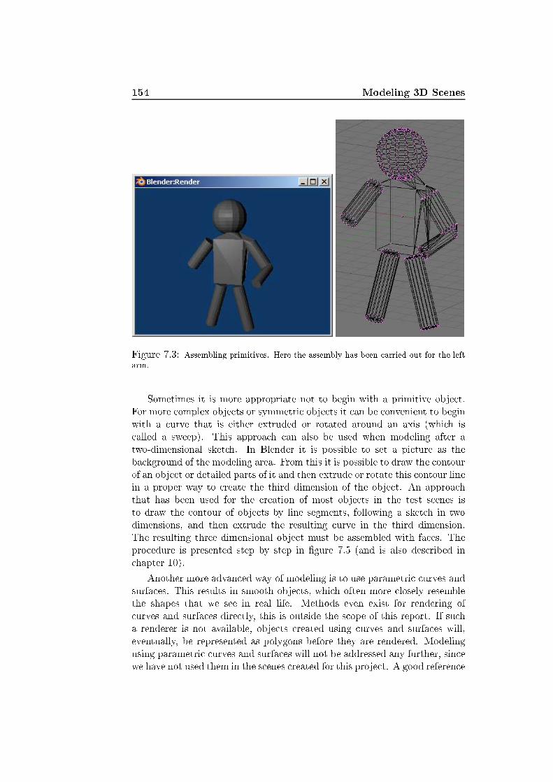
154 Modeling 3D S enes

Figure 7.3: Assembling primitives. Here the assembly has been arried out for the leftarm.Sometimes it is more appropriate not to begin with a primitive obje t.For more omplex obje ts or symmetri obje ts it an be onvenient to beginwith a urve that is either extruded or rotated around an axis (whi h is alled a sweep). This approa h an also be used when modeling after atwo-dimensional sket h. In Blender it is possible to set a pi ture as theba kground of the modeling area. From this it is possible to draw the ontourof an obje t or detailed parts of it and then extrude or rotate this ontour linein a proper way to reate the third dimension of the obje t. An approa hthat has been used for the reation of most obje ts in the test s enes isto draw the ontour of obje ts by line segments, following a sket h in twodimensions, and then extrude the resulting urve in the third dimension.The resulting three dimensional obje t must be assembled with fa es. Thepro edure is presented step by step in �gure 7.5 (and is also des ribed in hapter 10).Another more advan ed way of modeling is to use parametri urves andsurfa es. This results in smooth obje ts, whi h often more losely resemblethe shapes that we see in real life. Methods even exist for rendering of urves and surfa es dire tly, this is outside the s ope of this report. If su ha renderer is not available, obje ts reated using urves and surfa es will,eventually, be represented as polygons before they are rendered. Modelingusing parametri urves and surfa es will not be addressed any further, sin ewe have not used them in the s enes reated for this proje t. A good referen e

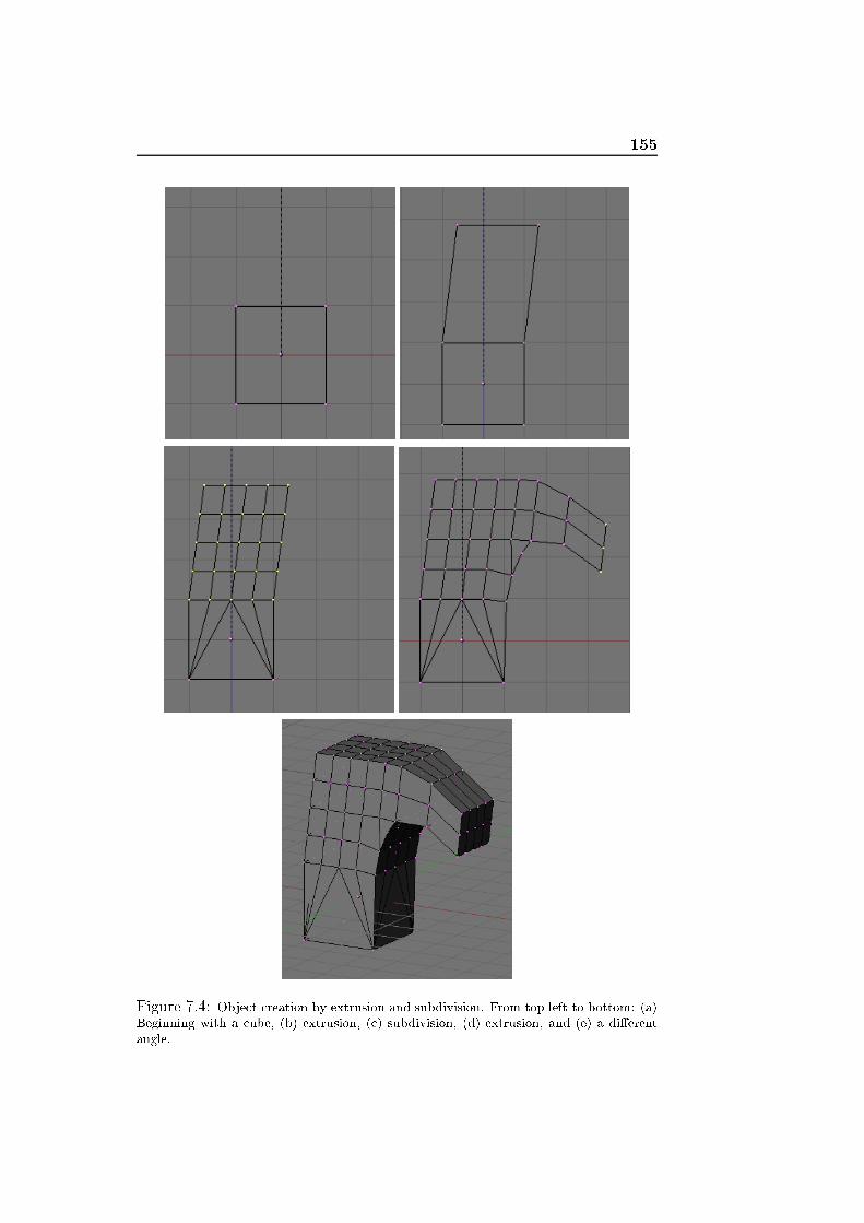
155

Figure 7.4: Obje t reation by extrusion and subdivision. From top left to bottom: (a)Beginning with a ube, (b) extrusion, ( ) subdivision, (d) extrusion, and (e) a di�erentangle.

156 Modeling 3D S enes

Figure 7.5: The line extrusion method. Contour of an obje t is drawn and then usedtogether with extrusions or rotations to omplete the 3D mesh.

157on usage of urves and surfa es for real-time rendering is [134℄.Above we have presented some di�erent basi approa hes to modelingpolygonal obje ts. None of these approa hes are more orre t to use thanothers (at least not to our knowledge), in the end a ombination of these and reativity is probably the best solution.The methods we des ribe may not be ustomary pro edure presentedin text books as parti ular ways of handling modeling issues, rather theyare omposed of the experien e with Blender obtained in this proje t andthrough di�erent tutorials found on the internet and in [113℄.When an obje t has been modeled the next step is to apply materialsand sometimes also textures. This is the subje t of the next hapter.

158 Modeling 3D S enes

Chapter 8Visual Appearan e

I often think that the night is more alive and more ri hly oloredthan the day. Vin ent Van Gogh (1853-1890)

160 Visual Appearan eAn important part of s ene reation is to de�ne material parameters forthe obje ts. Without material settings obje ts will never be ome realisti .As a general des ription you ould say that the material parameters simplyde ide how the light is re�e ted from the obje t. Still there are many issues insetting up the right material parameters. Often there are di�eren es betweenthe terms used in modeling appli ations and the terms used in theoreti altexts. This hapter will treat the basi material terms and relate them tothe theory presented in part I. Apart from material settings olor texturesalso play an important role. This is espe ially true for real-time appli ationswhere textures are often used to a hieve visual e�e ts that are otherwise tootime onsuming to simulate physi ally. Textures will be addressed shortlyat the end of this hapter.Se tion 8.1 will address olor settings in the RGB and HSV olor spa es.Besides the obje tive of the se tion is to des ribe what the meaning of amaterial olor is with respe t to light transport and s attering.The obje t olor is one thing, but it is far from the only fa tor in de�nitionof the material appearan e. What is also important, is how we per eivethe obje t material. Does the obje t appear soft, hard, shiny, et .? Theappearan e of an obje t in this sense very mu h depends on how the light isre�e ted from it. Se tion 8.2 will dis uss all material settings that are relatedto re�e tan e rather than olor. The se tion will introdu e some of the most ommonly used terms for material settings in modeling environments andrelate them to the di�erent material parameters that we have en ounteredwhile des ribing BRDFs in part I.Many global illumination e�e ts are simulated in real-time using textures.Textures are great tools for giving obje ts the �nal tou h of realism. Atexture an in a way be seen as a detailed painting of the obje t. Sometextures are more detailed than others. A texture an simply be a mix oftwo olors in a ertain pattern, for example to simulate wood grains or it an be detailed for example for the fa e of a hara ter. Se tion 8.3 shortlyintrodu es textures and their appli abilities.8.1 Colors and Human Per eptionWhen a light sour e illuminates an obje t the olor of the obje t is, in fa t, afun tion C(�) given by the produ t between the surfa e re�e tan e and thelight in ident on the obje t at di�erent wavelengths in the visible spe trum.Su h a olor fun tion is also alled the spe trum of the obje t. A briefdes ription of human per eption of olor is needed in order to explain whythree values are su� ient to model the ontinuous spe trum of an obje tFigure 8.1 shows a model of the human eye. The eye is very omplex andthere are many other things to it than what is shown here. The �gure onlyseeks to apture the most basi fun tionalities. In this report we an think

8.1 Colors and Human Per eption 161of the eye merely is a olle tor of light. The brain interprets the light thatthe eyes per eive and the results are the images that we see.

Lens

Iris

Cornea

Retina (Rods and Cones)

Optical nerve Figure 8.1: The eye alias the human visual system. (The �gure is inspired by �gure1.11 in [3℄.)The eye an be ompared to the pinhole amera presented in se tion2.3, it is more advan ed though. The ornea is a transparent prote tion ofthe eye. The iris adjusts the amount of light that is allowed to enter theeye, this is important sin e the retina is very sensitive to light. The iris isthe olored ring around the pupil and it is possible to observe its rea tionto light. If there is mu h light a smaller amount is allowed to enter. Thisis the reason why pupils get smaller in bright day light and larger in darksurroundings. The lens is omparable to the amera lens, it gathers lightfrom the surroundings and forms a 2 dimensional image on the ba kside ofthe eye alled the retina. The retina is overed with small rods and onesthat are able to translate the light into small impulses. These impulses aresent to the brain through the opti al nerve. The fun tionality of the eye istherefore only to gather information and pass it on to the brain. From hereit is the brain that must interpret what we see.The rods and ones are the light sensors of the eye. The rods olle tlight at low levels of density, hen e, they are responsible for night vision.The rods are good at olle ting small densities of light, but are not goodat determining the olor and shape of an obje t. Cones are responsible forday vision and an handle olors and shapes well, but they will only work ifsu� ient light is present.The ones are responsible for olle tion of olors. Exa tly how this hap-pens is still not fully understood, however, the eye has three di�erent onere eptors and it is ommonly a epted that the ones mainly absorbs threedi�erent olors: Red, green and blue [39℄. These are referred to as the pri-mary olors [38℄. In other words the brain re eive three signals from the eyeand must interpret a olor given by an otherwise ontinuous spe trum usingthese three signals only. �This is why three numbers an be used to represent

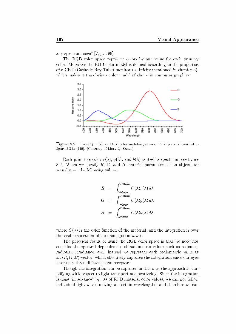
162 Visual Appearan eany spe trum seen� [2, p. 188℄.The RGB olor spa e represent olors by one value for ea h primary olor. Moreover the RGB olor model is de�ned a ording to the propertiesof a CRT (Cathode Ray Tube) monitor (as brie�y mentioned in hapter 3),whi h makes it the obvious olor model of hoi e in omputer graphi s.

Figure 8.2: The r(�), g(�), and b(�) olor mat hing urves. This �gure is identi al to�gure 2.3 in [119℄. (Courtesy of Mark Q. Shaw.)Ea h primitive olor r(�), g(�), and b(�) is itself a spe trum, see �gure8.2. When we spe ify R, G, and B material parameters of an obje t, wea tually set the following values:R = Z 780nm380nm C(�)r(�) d�G = Z 780nm380nm C(�)g(�) d�B = Z 780nm380nm C(�)b(�) d�where C(�) is the olor fun tion of the material, and the integration is overthe visible spe trum of ele tromagneti waves.The pra ti al result of using the RGB olor spa e is that we need not onsider the spe tral dependen ies of radiometri values su h as radian e,radiosity, irradian e, et . Instead we represent ea h radiometri value asan (R;G;B)-ve tor, whi h e�e tively aptures the integration sin e our eyeshave only three di�erent one re eptors.Though the integration an be aptured in this way, the approa h is sim-plifying with respe t to light transport and s attering. Sin e the integrationis done �in advan e� by use of RGB material olor values, we an not followindividual light waves moving at ertain wavelengths, and therefore we an

8.1 Colors and Human Per eption 163not model visual e�e ts that appear in wave opti s (su h as �uoros en e,phosphores en e, interferen e, and di�ra tion).Though onvenient with respe t to a omputer monitor, a modeler shouldbe aware that the RGB olor spa e an not model all visible olors. In 1931CIE (Commission Internationale d'E lairage) de�ned three standard primaryfun tions alled x(�), y(�), and z(�) from whi h all visible olors an bemat hed using only positive weights. They are meant to repla e r(�), g(�),and b(�), to avoid their short omings. This has not happened in omputergraphi s, sin e the RGB model �ts the monitors better.There are many di�erent olor spa es or models representing olors indi�erent ways. We an mention a few like CMYK, normally used in theprinting industry and in ink standards, and YIQ used in onne tion withtelevision. Some olor models are based on per eptual terms su h as hueand saturation. We will brie�y des ribe the two olor spa es RGB and HSV(hue, saturation, value), sin e they are both available in Blender.The RGB olor spa e an be visualized by the ube shown in �gure 8.3.Colors in the RGB room are simply generated by adding the di�erent valuesof red, green, and blue, whi h are de�ned as the primary olors.

Blue (0, 0, 1) Cyan (0, 1, 1)

Green (0, 1, 0) Black (0, 0, 0)

Red (1, 0, 0) Yellow (1, 1, 0)

Magenta (1, 0, 1) White (1, 1, 1)

Gray levels

Figure 8.3: The RGB olor spa e.The HSV model represents olors by hue, saturation, and a value. Herewe have a hexagonally shaped olor spa e, orresponding to a one subtendedby an isometri view of the RGB olor spa e, whi h means looking at the ube in �gure 8.3 from the top downwards with the gray s ale line as theline of sight. The HSV olor spa e is shown in �gure 8.4.Setting the value parameter in the HSV room is like setting the value(V ) between bla k and white, orresponding to movement along the grays ale line in RGB olor spa e. Hue (H) is an angle sele ting the pure olor,and saturation (S) has the per eptual meaning that we would expe t. Thismeans that S = 1 spe i�es pure olor a ording to H, while S = 0 is olorless

164 Visual Appearan e

Yellow

Red 0˚

Green 120˚

Blue 240˚

Cyan

Magenta

White (V = 1)

Black

V

H

S

S = 1

Gray level

Figure 8.4: The HSV olor spa e. This �gure is similar to �gure 13.30 in [38℄.gray.In this se tion it was des ribed why the three omponent olor theoryis most often employed in omputer graphi s, and the impa t of this theoryon light transport and s attering was brie�y mentioned. Figures 8.3 and8.4 provide a helpful overview of the olor spa es available in Blender. Thenext step is to des ribe other material settings whi h tell the BRDF how there�e ted light is distributed over the hemisphere. This is the subje t of thefollowing se tion.8.2 Material ParametersAn obje t an appear to be red and round, but this is not enough to des ribeit, for all that we know a red and round obje t ould be anything from a redapple to a red metal ball. The missing parameter is what some might referto as shininess. Is the obje t dull and disperse or is it shiny and re�e tive?Besides setting the olor of a material a ording to its re�e tan e atdi�erent wavelengths, there are also other parameters whi h are important.These parameters de ide whi h dire tions light in ident on a material froma ertain dire tion are s attered ba k into the environment. In other wordsthey de ide how di�use or how spe ular the re�e tan e of a material shouldbe. Su h parameters are, of ourse, related to the BRDF model used forshading.Looking at the di�erent BRDF models des ribed in hapter 5, it showsthat Phong shading and its variants are determined by three material pa-rameters:

8.2 Material Parameters 165kd The di�use re�e tan e.ks The spe ular re�e tan e.m The shininess.In pra ti e this means that the kd orresponds to the general dull RGB olor of an obje t. If the obje t is shiny and re�e tive it will have a highlightaround the dire tion where a perfe tly spe ular obje t would have re�e tedlight dire tly towards the viewer. ks de�nes the olor of the light re�e tedspe ularly in the highlight. m sets the size of the highlight. A very shinyobje t (with large m) has a small on entrated highlight. To avoid overex-posed light (meaning that the exitant radian e is larger than in ident at thematerial) it should generally be the ase that kd + ks � 1. In �gure 8.5 thee�e t of hange in the di�erent parameters is shown.

Figure 8.5: Changing material parameters asso iated with Phong variants. The kdde reases and the ks in reases orrespondingly in the verti al dire tion, going from topto bottom. In the horizontal dire tion we hange the value of the shininess parameter,starting to the left with a small value and ending to the right with a high value.Complex BRDF models su h as the Cook-Torran e and the Ward models,des ribed in se tion 6.5, mostly use a roughness parameter � rather thanshininess. We will not go into detail on these material parameters, sin e wehave mostly used Phong variants or the BRDF for perfe tly di�use materialswhere fr;d = kd = �d=�.

166 Visual Appearan eMaterials used for transmissive or translu ent solid obje ts need a fewextra parameters to be des ribed adequately. A perfe tly spe ular transmis-sive obje t, su h as glass, will merely need to have an index of refra tionspe i�ed. Re all from hapter 3 that translu ent obje ts also need to havean absorption oe� ient �a, an extin tion oe� ient �t, and a s attering oe� ient �s spe i�ed. Besides we need to spe ify a phase fun tion ratherthan a BRDF for translu ent material. For simpli ity we have hosen to workwith perfe tly di�use translu ent materials only in this proje t, whi h meansthat no material parameters, ex ept for the di�use obje t olor, is needed forthe phase fun tion. The relationship between the three oe� ients is that�t = �a+�s, whi h means that we need only spe ify two of them. Su h twoparameters an be measured, and they are given for di�erent materials inliterature (eg. in [65℄).When setting material properties in Blender two three omponent olorsshould be spe i�ed. They are spe i�ed either in the RGB or the HSV olorspa e (see the previous se tion, and see also hap. 10). Col is the di�use olor of an obje t and Spe is the spe ular olor of an obje t. Then Blenderhas a spe ular parameter spe 2 [0; 2℄, a shininess or roughness parameterhard 2 [1; 500℄, and a di�use re�e tan e parameter ref 2 [0; 1℄. Blenderallows overexposure of light. The following formulas translate the Blendermaterial parameters to kd, ks, and m. Blender also allows omplex BRDFsin whi h ase m simply repla es �:kd = Col � refks = EACH (1 min) (Spe � spe )m = hardBlender has a translu en y parameter whi h is explained in Blender as�the amount of di�use shading of the ba kside�. Supposedly it is used forsimulation of subsurfa e s attering. Dire t translation of this parameterto the absorption, s attering, and extin tion oe� ients is not immediatelypossible. More likely Blender translu en y spe i�es a onstant orrespondingto e�� , where � is the opti al depth of the obje t to whi h the material isapplied (see se . 3.4).The index of refra tion is alled IOR 2 [1; 3℄ in Blender, and otherparameters su h as transparen y A are also available. Transparen y spe i�esthe rate to whi h the obje t should be blended with the ba kground. Blenderalso allows the user to spe ify an ambient term Amb 2 [0; 1℄ and an emissionterm Emit 2 [0; 1℄. The ambient olor Col � Amb simulates multiple di�usere�e tions by a onstant and the emission term orresponds to a onstantLe emitted from the obje t to whi h the material is applied.Real materials are not perfe tly smooth and regularly olored over theentire surfa e. For example you will not be able to �nd any fully re�e tive

8.3 Textures 167surfa es in the real world. Therefore it often adds extra realism to a surfa eif the material olor hanges a ross it. This is often added by the use oftextures, whi h is the subje t of the next se tion.8.3 TexturesThe visual result of adding olor textures to a s ene is best des ribed byexample. To have more omplex show ases than a Cornell box, we have reated a ave s ene in Blender for this proje t. A s reen shot from the aves ene with no textures is given in �gure 8.6 and a s reen shot of the sameview in luding textures is given for omparison in �gure 8.7. Note that thetextures added in this s ene are very simple and that it is possible to use farmore ompli ated textures, this is, however, outside the s ope of this report.

Figure 8.6: S reen shot from the ave s ene with no textures (Blender render).Unfortunately we have not found time for adding textures to all ourBlender obje ts, and neither have we found the time to make a proper export

168 Visual Appearan e

Figure 8.7: S reen shot from the ave s ene in luding textures (Blender render).of textures in order to use them in our own rendering. Though olor textures an provide great visual e�e ts, they are of less importan e with respe t toillumination. A olor texture simply simulates that the RGB olor of anobje t varies a ross the surfa e.Textures are applied at a late stage in the rendering pipeline, see se tion5.1, and they have many di�erent appli abilities apart from olor texturing,some of those are des ribed in se tion 5.3. Often textures are used for storageof information, whi h is useful to have in a fragment program. This is theprimary usage of textures in our rendering method, see part III. Anotherinteresting appli ation of textures is light maps, whi h is des ribed in se tion6.6.We have now brie�y introdu ed the most important material settingsavailable in Blender and related them to theory in hapters 3 and 5. Thenext hapter will des ribe how obje ts are moved around in a s ene. Thisis important sin e the ability to make things move around and ome alive isthe main reason why we want real-time rendering.

Chapter 9Making Things Come Alive

24. And God said, Let the earth bring forth the living reatureafter his kind, attle, and reeping thing, and beast of theearth after his kind: and it was so.25. And God made the beast of the earth after his kind, and attle after their kind, and everything that reepeth upon theearth after his kind: and God saw that it was good.The Bible (King James Version): Gen.1 Verses 24 to 25

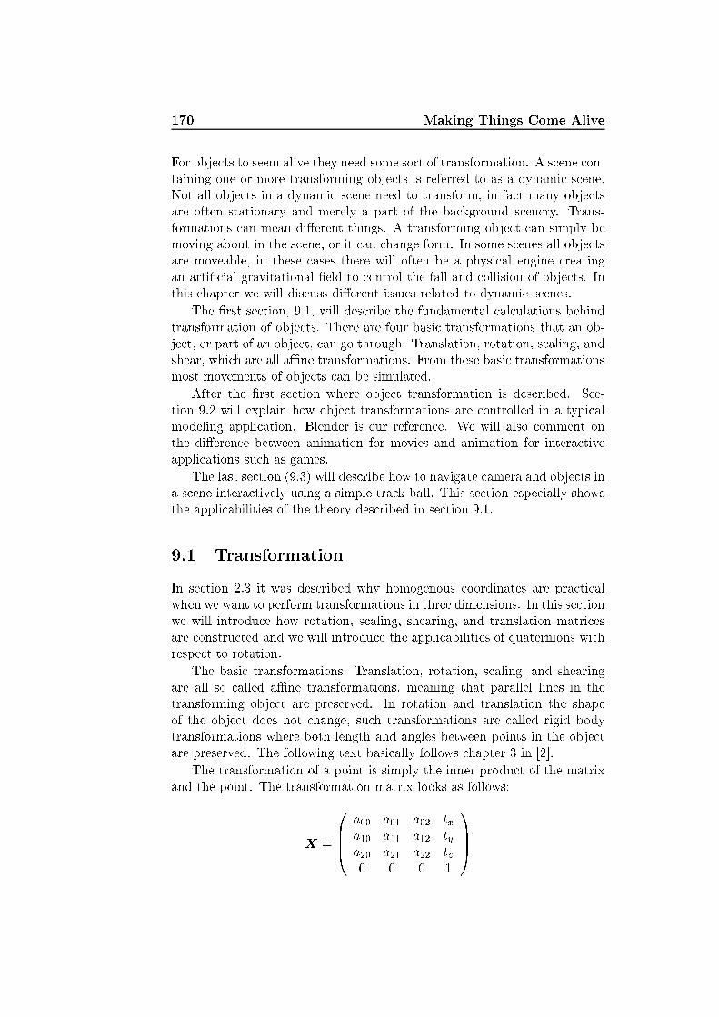
170 Making Things Come AliveFor obje ts to seem alive they need some sort of transformation. A s ene on-taining one or more transforming obje ts is referred to as a dynami s ene.Not all obje ts in a dynami s ene need to transform, in fa t many obje tsare often stationary and merely a part of the ba kground s enery. Trans-formations an mean di�erent things. A transforming obje t an simply bemoving about in the s ene, or it an hange form. In some s enes all obje tsare moveable, in these ases there will often be a physi al engine reatingan arti� ial gravitational �eld to ontrol the fall and ollision of obje ts. Inthis hapter we will dis uss di�erent issues related to dynami s enes.The �rst se tion, 9.1, will des ribe the fundamental al ulations behindtransformation of obje ts. There are four basi transformations that an ob-je t, or part of an obje t, an go through: Translation, rotation, s aling, andshear, whi h are all a�ne transformations. From these basi transformationsmost movements of obje ts an be simulated.After the �rst se tion where obje t transformation is des ribed. Se -tion 9.2 will explain how obje t transformations are ontrolled in a typi almodeling appli ation. Blender is our referen e. We will also omment onthe di�eren e between animation for movies and animation for intera tiveappli ations su h as games.The last se tion (9.3) will des ribe how to navigate amera and obje ts ina s ene intera tively using a simple tra k ball. This se tion espe ially showsthe appli abilities of the theory des ribed in se tion 9.1.9.1 TransformationIn se tion 2.3 it was des ribed why homogenous oordinates are pra ti alwhen we want to perform transformations in three dimensions. In this se tionwe will introdu e how rotation, s aling, shearing, and translation matri esare onstru ted and we will introdu e the appli abilities of quaternions withrespe t to rotation.The basi transformations: Translation, rotation, s aling, and shearingare all so alled a�ne transformations, meaning that parallel lines in thetransforming obje t are preserved. In rotation and translation the shapeof the obje t does not hange, su h transformations are alled rigid bodytransformations where both length and angles between points in the obje tare preserved. The following text basi ally follows hapter 3 in [2℄.The transformation of a point is simply the inner produ t of the matrixand the point. The transformation matrix looks as follows:X = 0BB� a00 a01 a02 txa10 a11 a12 tya20 a21 a22 tz0 0 0 1 1CCA

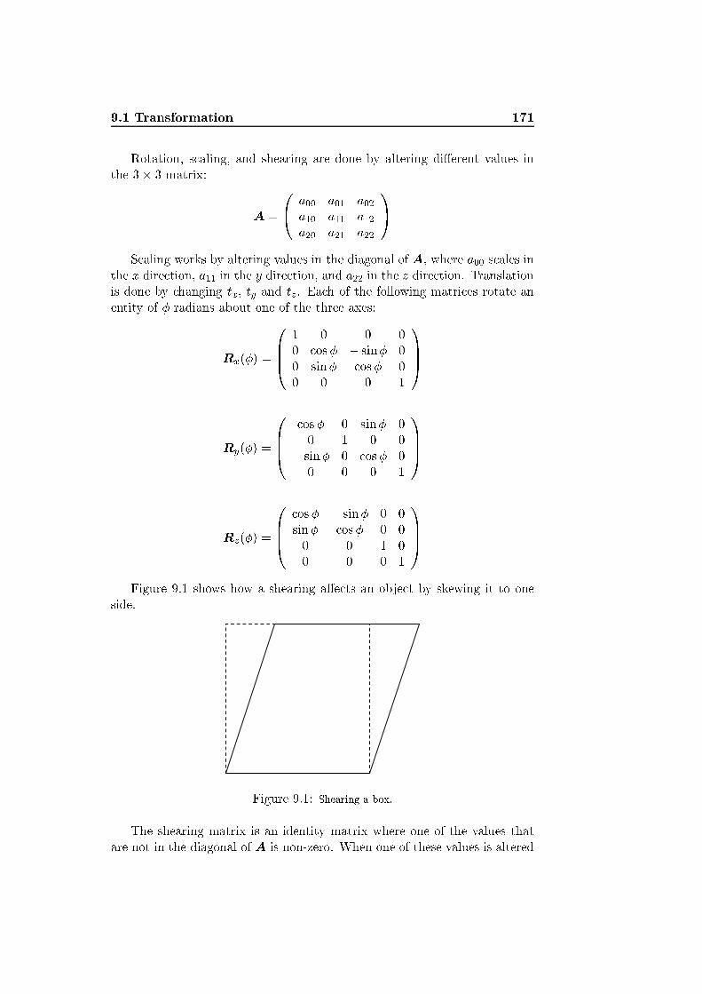
9.1 Transformation 171Rotation, s aling, and shearing are done by altering di�erent values inthe 3� 3 matrix: A = 0� a00 a01 a02a10 a11 a12a20 a21 a22 1AS aling works by altering values in the diagonal of A, where a00 s ales inthe x dire tion, a11 in the y dire tion, and a22 in the z dire tion. Translationis done by hanging tx, ty and tz. Ea h of the following matri es rotate anentity of � radians about one of the three axes:Rx(�) = 0BB� 1 0 0 00 os� � sin� 00 sin� os� 00 0 0 1 1CCARy(�) =0BB� os� 0 sin� 00 1 0 0� sin� 0 os� 00 0 0 1 1CCARz(�) = 0BB� os� � sin� 0 0sin� os� 0 00 0 1 00 0 0 1 1CCAFigure 9.1 shows how a shearing a�e ts an obje t by skewing it to oneside.

Figure 9.1: Shearing a box.The shearing matrix is an identity matrix where one of the values thatare not in the diagonal of A is non-zero. When one of these values is altered

172 Making Things Come Aliveit orresponds to shearing in one parti ular dire tion (positive or negative)on one parti ular axis.Several transformations an be gathered in a single transformation ma-trix. If an obje t should be rotated a bit a ording to a transformationmatrix R and then translated a bit a ording to a matrix T , the �nal trans-formation matrix X is found by matrix multipli ation of the translationmatrix and the rotation matrix: X = TRIn this way more omplex transformations an be reated still using onlyone transformation matrix. Noti e that R is applied �rst, but is writtenlast. The order in whi h the matri es are multiplied has in�uen e on the�nal out ome. This should be taken into onsideration when reating the�nal transformation matrix.The inverse transformation matrix is often useful, for example whenswit hing between oordinate systems. The general way for omputing theinverse of a matrix is given as explained in [2, p. 728℄ or any standard textbook on linear algebra (eg. [31℄). Another very useful way of omputinginverses is in the ase where A is an orthogonal matrix, whi h is always the ase if the transformation is a on atenation of translations and rotationsonly. The inverse of an orthogonal matrix is given as M�1 = MT , hen ethe inverse of X if A is orthogonal is given as:X�1ortho = 0BB� a00 a10 a20 �(t � (a00; a10; a20))a01 a11 a21 �(t � (a01; a11; a21))a02 a12 a22 �(t � (a02; a12; a22))0 0 0 1 1CCA (9.1)QuaternionsA ompa t and useful way to represent rotations is by use of a mathemati al on eption alled quaternions, introdu ed to omputer graphi s in [120℄. Wewill not des ribe the mathemati al ba kground of quaternions here, somereferen es are [2, 24, 42℄. Rather we will shortly introdu e their usage.A quaternion is represented by a four-tuple q = (qv ; qw) = (qx; qy; qz; qw),it should, however, not be onfused with homogenous oordinates. Opera-tions on quaternions are given as follows [2, p. 45℄:Multipli ation qr = (qv � rv + rwqv + qwrv; qwrw � qv � rv)Addition q + r = (qv + rv; qw + rw)Conjugate q� = (�qv; qw)Norm n(q) = q2x + q2y + q2z + q2wIdentity i = (0; 1)

9.2 Animation and Motion Control 173Suppose we have a point or a ve tor given in homogenous oordinatesp = (px; py; pz; pw). Let the quaternion p be given as ea h omponent of pinserted in p. Now, given a unit quaternion q = (sin�uq; os�), where uqis a ve tor representing an arbitrary axis, then:p 7! qpq�1 = qpq�n(q) = qpq� (9.2)rotates p (whi h orresponds to p) around the axis uq by an angle 2� [2℄.Note that for a unit quaternion it is the ase that q�1 = q�. It an be shownthat any rotation an be obtained in this manner, see eg. [42℄. This indi atesthat quaternions are a ompa t and e� ient way of representing rotation inthree-dimensional spa e.The rotation given above, (9.2), is also alled an adjoint map of p. It an also be shown (eg. [42℄) that this adjoint map has a orresponding 3� 3rotation matrix, whi h is orthogonal. Sin e we have only made use of unitquaternions in this proje t, we present the onversion from a unit quaternionq to a 3� 3 rotation matrix M q below. For the general formula we refer to[42, 2, 120℄.Aq = 0� 1� 2(q2y + q2z) 2(qxqy � qwqz) 2(qxqz + qwqy)2(qxqy + qwqz) 1� 2(q2x + q2z) 2(qyqz � qwqx)2(qxqz � qwqy) 2(qyqz + qwqx) 1� 2(q2x + q2y) 1A (9.3)Another interesting feature of a quaternion is the ease by whi h therotation from one ve tor to another an be spe i�ed. Let s and t be twounit ve tors denoting a dire tion in spa e. A unit rotation axis is then givenas u = (s � t)=ks � tk. If 2� denotes the angle between s and t, thens � t = os(2�) and ks � tk = sin(2�). �The quaternion that represents therotation from s to t is then q = (sin�u; os �)� [2, p. 51℄.A few trigonometri al ulations show that the formula �nding a unitquaternion spe ifying the rotation between two ve tors s and t is given as[2℄: q = (qv; qw) = 1p2(1 + s � t)(s� t);p2(1 + s � t)2 ! (9.4)This ends our presentation of transformations. In the following se tionswe will give some examples of their use.9.2 Animation and Motion ControlBuilding on the transformation matri es introdu ed in the previous se tion,we an reate a series of frames where di�erent transformation matri es are

174 Making Things Come Aliveused in order to give an obje t the appearan e of ontinuous movement.Su h a movement is referred to as animation. Animation an be a simplemovement, like a ball boun ing up and down, or it an be more omplex, likea person walking or a fa ial expressions. All movements over time qualify.Animation is normally done in a modeling appli ation by use of keyframes. Sin e the obje t is moving over time they need to be redrawn ina slightly di�erent position for ea h frame. Redrawing ea h moving obje tfor ea h frame would be an overwhelming task. With key frames only keytransforms of the obje ts moving are set, after that the appli ation omputesthe transformations of the frames in-between.A simple al ulation of obje t positions in-between key frames is by linearinterpolation. However to reate realisti transformations it is sometimesne essary that the movement is not linear. An example ould be a balljumping up and down. If the ball is to follow the laws of physi s, it willmove slower around its highest point and faster at set o� and just beforehitting the ground. To reate su h e�e ts we an use interpolation urves,whi h an be found using quaternion urves, see [120, 24℄. Movements likethis ould also be simulated by a physi s engine supporting gravity, whi h iswhy a good physi s engine an save a lot of animation time.In Blender key frames are ontrolled in the a tion viewer, where all keyframes are pla ed. By this view key positions of obje ts an easily be movedor opied to di�erent frames. Blender also supports interpolation urves inthe Ipo view.As we have seen in hapter 7, hara ters are often reated from one mesh.If hara ters are supposed to move body parts only (for example an arm ora leg), just some of the mesh an be moved instead of the entire obje t.For simulating walking, for instan e, parts of the hara ter mesh must bemoved in di�erent dire tions at the same time. For purposes like this we an reate a skeleton-like mesh de�ning bones that an be atta hed to partsof the mesh. Su h a skeleton is alled an armature. Whenever a bone inthe armature moves verti es atta hed to it will follow. In this way we anmodify only parts of the mesh in�uen ed by the bones. An example of anarmature an be seen in �gure 9.2.There is di�eren e between animations for a movie and animations for areal-time appli ation su h as a game. Ex ept for the fa t that movie anima-tions are mu h more detailed and spe ta ular, they are also predetermined.This means that the artist an on entrate on parti ular movements only.In a game, for example, movement of obje ts most often depends on how theuser intera ts with the s ene. The fa t that the exa t movement of obje tsin a real-time appli ation is unknown, means that animations must be splitup into smaller pie es, ea h ontaining movement we know will be useful inmany situations. Moreover animations like these must be able to follow ea hother in a �uent manner.Small animation snippets, like those des ribed above, are alled y les.

9.3 Intera tive Control 175

Figure 9.2: Armature of the male hara ter in the ave s ene. Noti e how the meshfollows the bones.In a game with a hara ter ontrolled by a user, y les su h as a walk y leor a hit y le ould be useful. In the example of a walk y le the animationsnippet must be able to `re- y le', meaning that if several walk y les followone another, they will appear as if the hara ter just kept walking.To have a moving light sour e in our ave s ene the hara ter shown in�gure 9.2 is supposed to walk about with a lantern, a walk y le was reatedfor this purpose and an idle y le. Unfortunately there has not been timeto export these animations to our own appli ation. In order to show thata s ene is truly dynami , we must also be able to alter it dynami ally. Inreal-time appli ations this usually happens by moving things around in thes ene using some sort of input devi e (mouse, keyboard, et .). Intera tive ontrol is the subje t of the next se tion.9.3 Intera tive ControlIn many real-time 3D appli ations a simple virtual tra k ball is onne tedto a mouse input devi e and used for amera navigation. This is also the

176 Making Things Come Alive ase for the appli ation implemented during this proje t. The tra k ball weuse was originally distributed during the DTU �Computer Graphi s� ourse(02561). During this proje t we have modi�ed the tra k ball from time totime and we have parti ularly adapted it to work for navigation of a hosenobje t (a ording to the urrent amera view) as well as it works for ameranavigation. In the following we will �rst des ribe how the tra k ball worksfor intera tive amera ontrol, and se ond we will des ribe our expansion ofit to in lude intera tive obje t ontrol.The tra k ball is initialized by a enter L around whi h the amera shouldrotate, and a distan e zeye whi h spe i�es how far away along the z-axis theeye point, or amera, should be pla ed. Most often the enter is de�ned asthe enter of the s ene in whi h the tra k ball is pla ed or the enter of aparti ular obje t in the s ene.Internally the tra k ball has a translation ve tor t = (tx; ty; tz) whi h isapplied in view spa e, meaning that altering (tx; ty) results in a pan motionof the amera, while altering tz results in a zoom motion. Pan motion isdes ribed by mouse motion when the right mouse button is down. Zoomis des ribed by the mouse moving forwards or ba kwards when the middlemouse button is down.The basis of the view spa e oordinate system is given by the urrentrotation of the amera. This rotation is spe i�ed by a quaternion qrot. Mov-ing the mouse while the left button is down will ea h frame provide a newmouse position to the tra k ball. This mouse position is proje ted to thesphere representing the virtual tra k ball. The sphere (or ball) is lo ated atthe enter of the s ene in view spa e, that is, the position the amera willalways be pointing at. The new position found on the sphere will spe ify anew viewing dire tion v2. Suppose the previous viewing dire tion was storedas v1, then the quaternion qin spe ifying the rotation from v1 to v2 is givenby (9.4).As des ribed in se tion 5.1, eye point E, `look-at' point L, and up ve torvup are su� ient to des ribe the amera orientation. If we hoose the defaultorthonormal basis for the amera orientation (ex;ey;ez), the amera eyepoint, `look-at' point, and up ve tor are given as:vup = qroteyq�rotL = tyvup + txqrotexq�rotE = qrot((zeye + tz)ez)q�rot + Lwhere ea h resulting quaternion orresponds to a ve tor or a point in ho-mogenous oordinates.Now, all we need to do in order to rotate the amera in rementally a - ording to the mouse motion, is to al ulate qrot := qrotqin for ea h frame.We an even let the amera spin a ording to a previous motion after the

9.3 Intera tive Control 177left mouse button has been released by storing the in remental quaternionqin . The spin stops when qin is reset to quaternion identity.The extension for this tra k ball is to freeze the amera when the userpi ks an obje t (eg. by pressing `p' when the mouse is lo ated over an obje t),and then let the mouse ontrol the sele ted obje t instead of the amera.What we want to spe ify with the mouse is the modeling transform (see �g.5.1) of the sele ted obje t.In order to move an obje t intuitively with the mouse, the motion shouldbe ontrolled in view spa e, sin e this is the spa e where the user works. Thetask is now to �nd the modeling transform in view spa e.When the tra k ball is frozen we store the old view transformation matrixspe i�ed by E, L, and vup (how to �nd the matrix from these three isdes ribed in se tion 5.1). If we let Mview denote the view transform, then atransformation X arried out in view spa e is given in world spa e as:Xworld =M�1viewXviewMview (9.5)Lu kily the view spa e transformation onsist of translation and rotationof the amera only, therefore we an �nd M�1view using (9.1).Setting the enter of the tra k ball to the enter of the obje t in worldspa e Cworld, we an spe ify the translation of the obje t in view spa e Tviewa ording to pan and zoom of the tra k ball:Tview = 0BB� 1 0 0 tx0 1 0 ty0 0 1 tz0 0 0 1 1CCAwhere pan be omes moving the obje t parallel to the view plane and zoombe omes moving the obje t along the dire tion from the urrent ameraposition to the obje t enter. This results in a quite intuitive translationof the obje t a ording to mouse movement. The next step is to rotate theobje t.In order to rotate the obje t intuitively in view spa e we must �rst moveit to the origin of the view spa e oordinate system. Having the enter ofthe obje t in world spa e oordinates Cworld, we an transform it to viewspa e oordinates as follows:Cview =MviewCworldThe translation is then simple be ause the origin of the view spa e oor-dinate system is now in (0; 0; 0) relative to Cview. Translation of the obje tto the origin of view spa e is:Tview;�C = 0BB� 1 0 0 �Cview;x0 1 0 �Cview;y0 0 1 �Cview;z0 0 0 1 1CCA

178 Making Things Come Aliveand translation ba k to the previous obje t position is:Tview;C = 0BB� 1 0 0 Cview;x0 1 0 Cview;y0 0 1 Cview;z0 0 0 1 1CCASin e we are looking at the obje t along the z-axis in view spa e, the lo al oordinate system around whi h we want to rotate the obje t will have a z-axis pointing in the opposite dire tion. If the obje t was positioned exa tlyin the `look-at' point, the basis of the obje t oordinate system would beexa tly opposite the basis of the view spa e oordinate system. Therefore,when we rotate the tra k ball, a reasonable approximation to a rotationof the sele ted obje t instead of the amera is given in view spa e as the onversion of q�1rot = q�rot to a rotation matrix M q�rot a ording to (9.3).The rotation should as mentioned be performed at the origin of viewspa e. The �nal transformation of the obje t in view spa e is, therefore,given as: Xview = TviewTview;CM q�rotTview;�C (9.6)Inserting (9.6) in (9.5) results in the transform of the obje t in worldspa e. If the obje t had no modeling transform to begin with. We an letXworld spe ify the new modeling transform of the obje t. For this proje t wewill always assume that the obje t has no other modeling transform whenthis tra k ball motion ontrol is applied.This hapter has introdu torily shown the impa t of intera tion and an-imation on real-time graphi s. In the following hapter we will give a brieftutorial on Blender modeling, sin e one part of this proje t has been to showthe work �ow from modeling to rendering.

Chapter 10Modeling in Blender r

�Well� said Owl, �the ustomary pro edure in su h ases is asfollows.��What does Crustimoney Proseed ake mean?� said Pooh. �For Iam a Bear of Very Little Brain, and long words bother me.��It means the Thing to Do.��As long at it means that, I don't mind,� said Pooh humbly.A. A. Milne (1926): Winnie-the-Pooh

180 Modeling in Blender r After introdu ing some of the di�erent aspe ts in modeling we turn to themodeling appli ation. As mentioned before we have used a modeling appli- ation alled Blender to reate most of our test s enes. One of the obje tivesof this proje t is also to reate a platform for game reators with little orno �nan ial means. Being free of harge Blender plays an important rolein this obje tive. In this hapter we will give an introdu tion to the basi fun tionalities in Blender. It is des ribed how a tions related to the above hapters su h as obje t modeling, material and texture settings, and anima-tion are arried out. Blender has many fun tionalities in addition to thosedes ribed here, for knowledge about these and more advan ed features werefer to www.blender.org, whi h holds many ex ellent tutorials. A few ofthe additional fun tionalities will be mentioned at the end of the hapterwithout any details.During the proje t a newer version of Blender was released. This hapterbuilds on Blender 2.33a whi h is urrently the newest version available, butmany of the s enes were originally reated using Blender 2.24. We havefound no problems in using the newer version of Blender for the last partof the proje t though we might have missed some of the improvements that ould have eased our work.First step is to give an overview of the menus and windows in Blender.Se tion 10.1 will introdu e all the most important menus and views of theBlender workspa e. This se tion will also des ribe how to hange the viewin order to navigate in the s ene, and how to set up the amera.Se tion 10.2 will des ribe how models are reated from primitives, orpolygon by polygon, and transformed.After reating obje ts the next step is to give them material properties inorder to make them look more realisti . Se tion 10.3 will des ribe the basi material and texture fun tionalities in Blender.Following the order of hapters in this part, the next se tion (10.4) willaddress animation in Blender.When a s ene has been reated in Blender, we want to export it toour own render appli ation. This is the subje t of se tion 10.5, whi h willdes ribe how to use the export s ript that we have found for export fromBlender to the .x3d �le format. The import of .x3d �les to our own appli a-tion will also brie�y be mentioned.The last se tion (10.6) of this hapter will mention some of the additionalfeatures available in Blender. No details will be provided.10.1 Blender NavigationOpening Blender for the �rst time an be quite onfusing. The user interfa e(see �gure 10.1) has a vast amount of buttons and panels.For this se tion the most important window will be the one in the middle

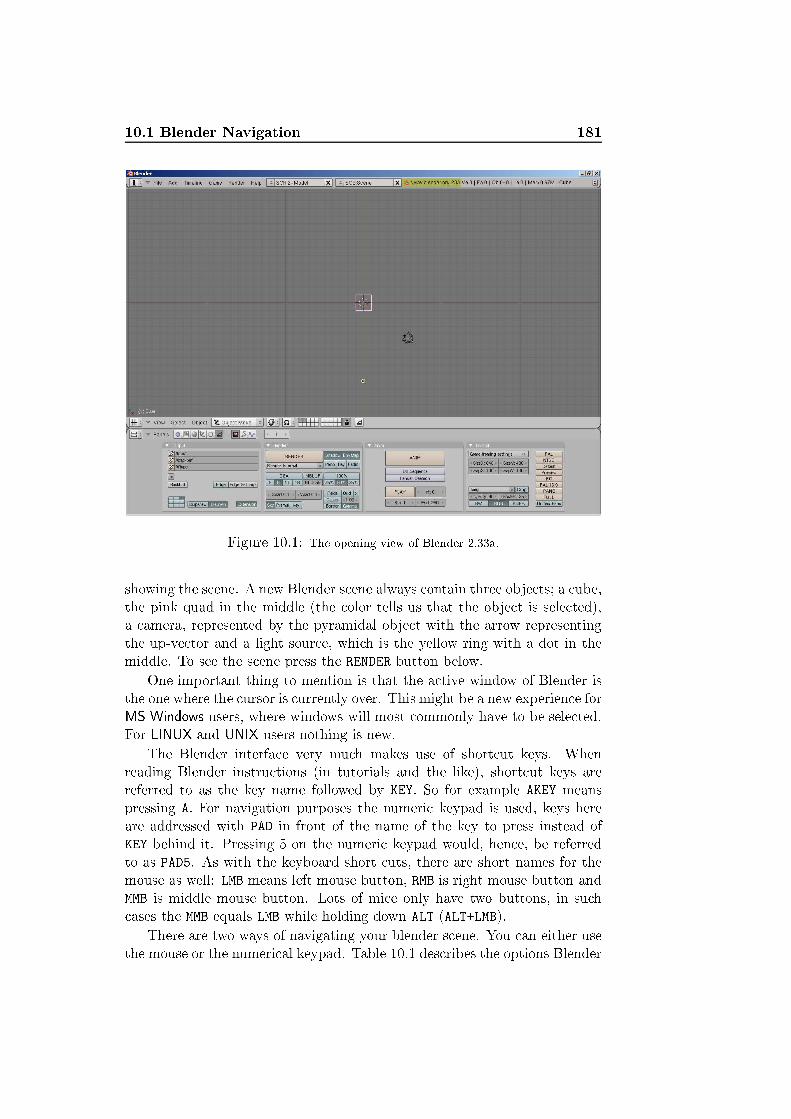
10.1 Blender Navigation 181

Figure 10.1: The opening view of Blender 2.33a.showing the s ene. A new Blender s ene always ontain three obje ts; a ube,the pink quad in the middle (the olor tells us that the obje t is sele ted),a amera, represented by the pyramidal obje t with the arrow representingthe up-ve tor and a light sour e, whi h is the yellow ring with a dot in themiddle. To see the s ene press the RENDER button below.One important thing to mention is that the a tive window of Blender isthe one where the ursor is urrently over. This might be a new experien e forMS Windows users, where windows will most ommonly have to be sele ted.For LINUX and UNIX users nothing is new.The Blender interfa e very mu h makes use of short ut keys. Whenreading Blender instru tions (in tutorials and the like), short ut keys arereferred to as the key name followed by KEY. So for example AKEY meanspressing A. For navigation purposes the numeri keypad is used, keys hereare addressed with PAD in front of the name of the key to press instead ofKEY behind it. Pressing 5 on the numeri keypad would, hen e, be referredto as PAD5. As with the keyboard short uts, there are short names for themouse as well: LMB means left mouse button, RMB is right mouse button andMMB is middle mouse button. Lots of mi e only have two buttons, in su h ases the MMB equals LMB while holding down ALT (ALT+LMB).There are two ways of navigating your blender s ene. You an either usethe mouse or the numeri al keypad. Table 10.1 des ribes the options Blender

182 Modeling in Blender r gives for s ene navigation.Key Fun tionalityPAD/ Show lo al view of sele ted obje ts (hide the rest of thes ene)PAD* Copy the rotation of the sele ted obje t to the urrent 3DwindowPAD- Zoom outPAD+ Zoom inPAD. Center and zoom in on sele ted obje tPAD5 Swit h between perspe tive and orthogonal viewPAD9 For e omplete re al ulation and redrawing of s ene andanimationsPAD0 Show amera view of the urrent a tive ameraCTRL-PAD0 Set urrent amera. Note that any obje t an be set as ameraALT-PAD0 Return to previous amera (only works with amera ob-je ts)PAD7 Top viewSHIFT-PAD7 Down view (opposite top view)PAD1 Front viewSHIFT-PAD1 Ba k viewPAD3 Right viewSHIFT-PAD3 Left viewPAD2 Rotate downwardsPAD8 Rotate upwardsPAD4 Rotate leftPAD6 Rotate rightSHIFT-PAD2 Translate downSHIFT-PAD8 Translate upSHIFT-PAD4 Translate leftSHIFT-PAD6 Translate rightMMB Rotation (tra k ball or axis aligned)1SHIFT-MMB TranslationCTRL-MMB Zoom2Table 10.1: Short uts for navigation in Blender.Blender has fourteen di�erent views that ea h an be hosen through1Whether it should be tra k ball or axis aligned rotation is set in the user menu. Theuser menu is found when dragging down the top menu under �Views & Controls�. Otherinteresting settings are found in here as well.2If you have a s roll mouse the s roll button will usually be atta hed to the zoomfun tionality as well.

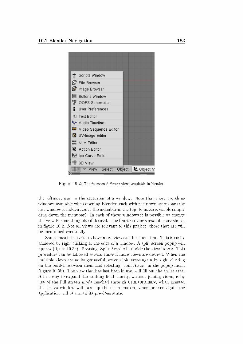
10.1 Blender Navigation 183

Figure 10.2: The fourteen di�erent views available in blender.the leftmost i on in the statusbar of a window. Note that there are threewindows available when opening Blender, ea h with their own statusbar (thelast window is hidden above the menubar in the top, to make it visible simplydrag down the menubar). In ea h of these windows it is possible to hangethe view to something else if desired. The fourteen views available are shownin �gure 10.2. Not all views are relevant to this proje t, those that are willbe mentioned eventually.Sometimes it is useful to have more views at the same time. This is easilya hieved by right li king at the edge of a window. A split s reen popup willappear (�gure 10.3a). Pressing �Split Area� will divide the view in two. Thispro edure an be followed several times if more views are desired. When themultiple views are no longer useful, we an join areas again by right li kingon the border between them and sele ting �Join Areas� in the popup menu(�gure 10.3b). The view that has last been in use, will �ll out the entire area.A fast way to expand the working �eld shortly, without joining views, is byuse of the full s reen mode rea hed through CTRL+UPARROW, when pressedthe a tive window will take up the entire s reen, when pressed again theappli ation will return to its previous state.

184 Modeling in Blender r

Figure 10.3: From left to right: (a) Splitting areas. (b) Joining areas.

Figure 10.4: Camera settings. Remember to have the amera sele ted and to sele t theedit panel.The s ene is made visible through the amera and is illuminated by thelight sour e. The amera an be moved about and rotated like any otherobje t in the s ene, how this is done is des ribed in the next se tion. Whena amera is sele ted (obje ts are sele ted with RMB) the amera parameters an be set. To set up the amera go to the edit panel by pressing F9 orsele ting the i on with a quad and four dots marking its orners (see �gure10.4).The amera settings are available in the amera panel (marked on �gure10.4). Here you are able to set the lens angle (�Lens�), whi h determs the �eldof view. Near and far lipping planes (�ClipSta� and �ClipEnd� respe tively) an also be set. �DrawSize� is simply the size of the amera obje t on thes reen. �Ortho� enables orthographi rendering, while �Show Limits� and�Show Mist� makes the boundaries of the visible area show in the modelingview.

10.2 Modeling in Blender 185Normally one amera is su� ient, but it is possible to have several am-eras pla ed in di�erent lo ations with the right settings ready. Renderingthen happens through the amera urrently a tive. To set another ameraa tive, simply sele t the amera and press CTRL+PAD0. Then the urrent amera is the sele ted one. A tually all obje ts an be hosen as a ameralike this, even though they are not a amera obje t. Be aware, though, that amera settings only are available if the obje t set as urrent amera is a amera obje t.Other small features and short ut keys that are ni e to know are pre-sented in tables 10.2 and 10.3.This se tion has des ribed the rux of the tools needed for Blender nav-igation. Many fun tionalities, buttons, panels, and views have not been de-s ribed here. To des ribe all the di�erent fun tionalities would be going toofar. More ex ellent tutorials and information an be found at www.blender.org.This is where the modeling appli ation also an be a quired. The followingse tion will give a short tutorial on modeling in Blender related to the re-ation of models for this proje t.10.2 Modeling in BlenderThe te hniques used for modeling in this proje t have already been des ribedin hapter 7. The purpose of this hapter is to des ribe how these te hniquesare arried out in Blender.The initial Blender s ene already ontains a amera, a light sour e, anda ube. The ube is sele ted, whi h is indi ated by its purple olor. Theability to sele t obje ts is, of ourse, ru ial. Table 10.4 will explain thedi�erent possibilities of obje t sele tion.The �rst modeling method in hapter 7 suggests use of primitives. Theeasiest way to add new primitives is to press SPACE in the modeling view.By this a tion you get the add menu, sele t the �Add!Mesh� submenu andpi k the primitive you would like to add (see �gure 10.5). The new primitivewill be pla ed where the enter is urrently pla ed.Obje ts an be moved around in the s ene arbitrarily, or rotated, ors aled. The di�erent possible obje t transformations an be seen in table10.5. All transformations will be arried out on the sele ted obje ts.After the short ut key has been pressed the obje t will follow the mouseuntil LMB is pressed. If RMB is pressed the transformation will be an eled. To ontrol transformations better hold down the CTRL key before the mouse ismoved. Now the obje t will only transform in a unit grid. Appropriate units3Paint sele tion provides the user with a brush like area to sele t obje ts. The area an be resized using the zoom fun tions or a s roll button. This sele tion feature is onlyavailable in edit mode (dis ussed later). To end paint sele tion mode press RMB.

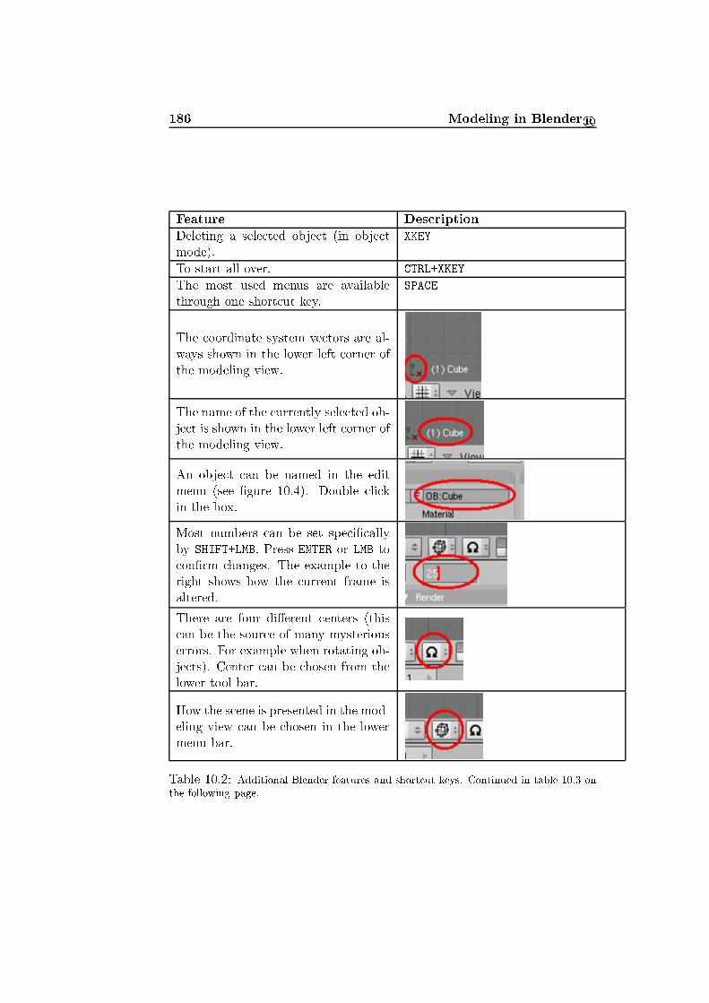
186 Modeling in Blender r Feature Des riptionDeleting a sele ted obje t (in obje tmode). XKEYTo start all over. CTRL+XKEYThe most used menus are availablethrough one short ut key. SPACEThe oordinate system ve tors are al-ways shown in the lower left orner ofthe modeling view.

The name of the urrently sele ted ob-je t is shown in the lower left orner ofthe modeling view. An obje t an be named in the editmenu (see �gure 10.4). Double li kin the box.

Most numbers an be set spe i� allyby SHIFT+LMB. Press ENTER or LMB to on�rm hanges. The example to theright shows how the urrent frame isaltered. There are four di�erent enters (this an be the sour e of many mysteriouserrors. For example when rotating ob-je ts). Center an be hosen from thelower tool bar. How the s ene is presented in the mod-eling view an be hosen in the lowermenu bar. Table 10.2: Additional Blender features and short ut keys. Continued in table 10.3 onthe following page.

10.2 Modeling in Blender 187Modes an be sele ted throughthe mode sele tion bar.

To view the s ene output we an use Blender's render en-gine. The rendering settingsappear by pressing F10. Torender an image from the ur-rent amera press the RENDERbutton in the middle menu. Undo is not really available,instead auto save is enabled.Auto save settings are foundby dragging down the topmenu bar and sele t auto save. If there is doubt about whata button does, a small helppopup will appear in many ases if the mouse is heldover the button for a shorttime (the example to the rightshows the help text for subdi-vision). Table 10.3: Additional Blender features and short ut keys. Continued from table 10.2on the previous page.Sele tion Type Short ut KeySele t obje t RMBSele t additional obje t SHIFT+RMBDesele t obje t SHIFT+RMB (on sele ted obje t)Desele t all obje ts AKEYSele t all obje ts AKEY (when none sele ted)Area drag sele tion BKEY then LMB (hold in and drag)Area drag de-sele tion BKEY then RMB (hold in and drag)Paint sele tion3 BKEY twi e - LMB sele tsPaint de-sele tion3 BKEY twi e - SHIFT+RMB de-sele tsTable 10.4: Sele ting obje ts in Blender.

188 Modeling in Blender r

Figure 10.5: The easiest way to add a new primitive. The menu pops up when SPACEis pressed.Obje t Transformation Short ut keyTranslation GKEYRotation RKEYS aling SKEYMirror MKEYTable 10.5: Blender transformations

10.2 Modeling in Blender 189 Figure 10.6: Units of transformation. This example is from s aling.

Figure 10.7: Settings for what should be visible in edit mode (NSize is the length of thenormals).are shown in the lower left orner (see �gure 10.6). Rotations will always bein the same plane as the view is in.It is also possible to restri t transformations like translation and s alingto follow an axis. After pressing the wanted transformation press the XKEY,YKEY, or ZKEY to sele t whi h axis to follow.To manipulate single (or more) verti es you will have to enter edit mode.To enter edit mode press TAB. Now all verti es are visible. Verti es anbe transformed and sele t in the same way as obje ts. When verti es aremanipulated triangles between them will automati ally follow.In edit mode it is possible to view fa es and normals. Settings for what tobe visible an be found under the edit menu (the same button as for settingup the amera, see �gure 10.4 in se tion 10.1), these settings an be seen in�gure 10.7.A small remark about the enter of the obje t marked by a small dot(pink when the obje t is sele ted and yellow when desele ted): When verti esare transformed in edit mode, the enter stays where it is, while outside editmode it follows the transformations. Therefore it is advisable not to translatethe entire obje t in edit mode unless you want to move the enter. Anotherimportant thing is that the enter will stay, representing the obje t even if allverti es are removed. In other words an obje t annot be deleted ompletely

190 Modeling in Blender r Figure 10.8: Features available in edit mode.in edit mode, always do this in obje t mode if the obje t should be entirelyremoved.Apart from the transformations available for obje ts, there are some extrapossibilities in edit mode for manipulating verti es also found under the editmenu. Some worth noti ing are: The �Set Smooth� option whi h smoothesthe obje t (�Set Solid� reverses this), �Subdivide� whi h subdivide sele tedverti es, �Extrude� generating an extrusion from sele ted surfa es (short utkey is the EKEY) and �Rem Double� adding together sele ted verti es lying lose to ea h other. Another good feature is the �Hide�/�Reveal� fun tional-ity. Using these buttons sele ted verti es an be temporarily hidden, whi hmakes it easier to manipulate verti es in more omplex meshes. Note alsothe �Double Sided� button, whi h is sele ted by default. Double sided meansthat fa es are visible from both sides. This an be a problem, sin e, for ex-ample, shadow volume al ulations only works for one-sided fa es, whi h an reate troubles when using obje ts outside Blender. Besides it is ru ial thatall fa es have the orre t orientation if we want do ba k fa e ulling, whi hwe always want to do if possible. A good advi e is therefore to desele t thisfeature. All features mentioned in this paragraph are outlined in �gure 10.8.Another method, whi h was des ribed in hapter 7, is to model after atwo-dimensional sket h. Loading a pi ture into the ba kground of Blenderis done as follows: Sele t �Ba kground Image. . . � in the view menu in thelower sele tion bar (�gure 10.9). The dialog shown in �gure 10.10 will appear.�Use Ba kground Image� reveals the other buttons and enables the use ofa ba kground image. To sele t an image press the folder i on to the rightof �Image:�. �Blend� determines transparen y of the image (0 equals notransparen y and 1 makes the image invisible). �Size� sets the size of theimage �X O�set� and �Y O�set� pla es the image in the s ene.The image remains at the same position from all angles, meaning that nomatter whi h angle you hoose to see the s ene the image will not transform.It is like a wall paper in the ba kground. The image will only be visible whenthe view is perpendi ular to one of the axes (PAD7, PAD1, PAD3, CTRL+PAD7,CTRL+PAD1, or CTRL+PAD3).In the following we will des ribe an example of modeling a ording to aba kground image. This is the method we have used for most of the obje ts reated for our test s ene. We will follow the example pi tured in �gure 7.5.

10.2 Modeling in Blender 191

Figure 10.9: Sele t �Ba kground Image. . . � to load an image into the Blender ba k-ground.

Figure 10.10: The �Ba kground Image� dialog.

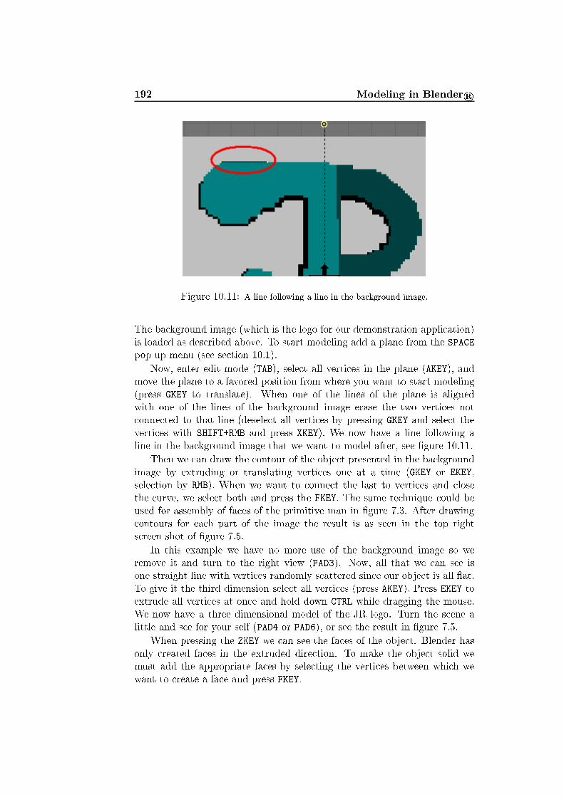
192 Modeling in Blender r

Figure 10.11: A line following a line in the ba kground image.The ba kground image (whi h is the logo for our demonstration appli ation)is loaded as des ribed above. To start modeling add a plane from the SPACEpop up menu (see se tion 10.1).Now, enter edit mode (TAB), sele t all verti es in the plane (AKEY), andmove the plane to a favored position from where you want to start modeling(press GKEY to translate). When one of the lines of the plane is alignedwith one of the lines of the ba kground image erase the two verti es not onne ted to that line (desele t all verti es by pressing GKEY and sele t theverti es with SHIFT+RMB and press XKEY). We now have a line following aline in the ba kground image that we want to model after, see �gure 10.11.Then we an draw the ontour of the obje t presented in the ba kgroundimage by extruding or translating verti es one at a time (GKEY or EKEY,sele tion by RMB). When we want to onne t the last to verti es and losethe urve, we sele t both and press the FKEY. The same te hnique ould beused for assembly of fa es of the primitive man in �gure 7.3. After drawing ontours for ea h part of the image the result is as seen in the top rights reen shot of �gure 7.5.In this example we have no more use of the ba kground image so weremove it and turn to the right view (PAD3). Now, all that we an see isone straight line with verti es randomly s attered sin e our obje t is all �at.To give it the third dimension sele t all verti es (press AKEY). Press EKEY toextrude all verti es at on e and hold down CTRL while dragging the mouse.We now have a three dimensional model of the JR logo. Turn the s ene alittle and see for your self (PAD4 or PAD6), or see the result in �gure 7.5.When pressing the ZKEY we an see the fa es of the obje t. Blender hasonly reated fa es in the extruded dire tion. To make the obje t solid wemust add the appropriate fa es by sele ting the verti es between whi h wewant to reate a fa e and press FKEY.

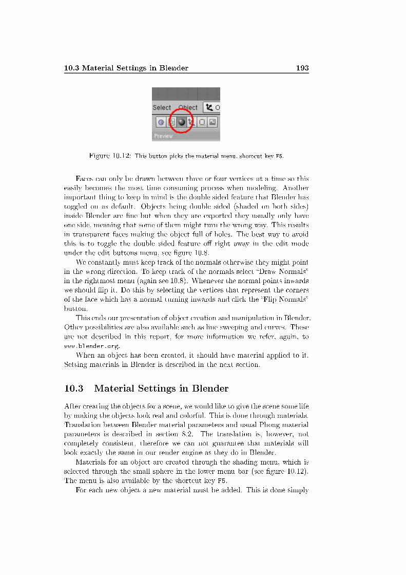
10.3 Material Settings in Blender 193 Figure 10.12: This button pi ks the material menu, short ut key F5.Fa es an only be drawn between three or four verti es at a time so thiseasily be omes the most time onsuming pro ess when modeling. Anotherimportant thing to keep in mind is the double sided feature that Blender hastoggled on as default. Obje ts being double sided (shaded on both sides)inside Blender are �ne but when they are exported they usually only haveone side, meaning that some of them might turn the wrong way. This resultsin transparent fa es making the obje t full of holes. The best way to avoidthis is to toggle the double sided feature o� right away in the edit modeunder the edit buttons menu, see �gure 10.8.We onstantly must keep tra k of the normals otherwise they might pointin the wrong dire tion. To keep tra k of the normals sele t �Draw Normals�in the rightmost menu (again see 10.8). Whenever the normal points inwardswe should �ip it. Do this by sele ting the verti es that represent the ornersof the fa e whi h has a normal turning inwards and li k the �Flip Normals�button.This ends our presentation of obje t reation and manipulation in Blender.Other possibilities are also available su h as line sweeping and urves. Theseare not des ribed in this report, for more information we refer, again, towww.blender.org.When an obje t has been reated, it should have material applied to it.Setting materials in Blender is des ribed in the next se tion.10.3 Material Settings in BlenderAfter reating the obje ts for a s ene, we would like to give the s ene some lifeby making the obje ts look real and olorful. This is done through materials.Translation between Blender material parameters and usual Phong materialparameters is des ribed in se tion 8.2. The translation is, however, not ompletely onsistent, therefore we an not guarantee that materials willlook exa tly the same in our render engine as they do in Blender.Materials for an obje t are reated through the shading menu, whi h issele ted through the small sphere in the lower menu bar (see �gure 10.12).The menu is also available by the short ut key F5.For ea h new obje t a new material must be added. This is done simply

194 Modeling in Blender r

Figure 10.13: Adding a new material.

Figure 10.14: Main Blender material settings.by pressing add new in the material menu, see �gure 10.13.When a new material is added a whole bun h of new options appear. Inthe following we will des ribe some of them.Like obje ts, materials an be named under the material settings in theMA �eld, where most other fun tionalities on erning olor and appearan eare found. Here the di�use olor �Col� and the spe ular olor �Spe� of anobje t are set. Note that it is possible to set olors using either the RGB orthe HSV olor spa e as des ribed in 8.1. The �DYN� button a tivates physi- al settings related to the material and the �Wire� button enables renderingin wire frame mode. �A� is transparen y settings. See �gure 10.14.In the �Shaders� menu all settings regarding ray tra ing are found. Herethere is also a slider for re�e tan e whi h is further outlined under the mirrortransparen y menu. Last we have the texture settings. Most hanges in thematerial settings are made visible in the preview menus in the left side part of

10.3 Material Settings in Blender 195 Figure 10.15: The texture menu. The right set of menu sele tion i ons appear only whenthe �rst material i on in the permanent set of menu sele tion i ons have been hosen.

Figure 10.16: Textures are set up in the �Texture� menu. Ea h texture refers by nameto textures added under the material menus. From left to right: (a) The texture menu ofthe material view. (b) The texture i on menu.the s reen. Sin e we are using our own renderer these are not too importantto us.The rightmost menu is for textures, that is, for asso iating textures witha material. This is done by pressing the �Add New� button. When thisbutton is pressed more menus will appear. They hold settings for how thetexture is mapped to an obje t to whi h the material is applied. How thetexture should look, is set up in yet another set of menus, whi h are foundin the menu bar above the extra set of menu i ons that appear when thematerial setting have been hosen. Instead of the red sphere hoose theleopard skin. See �gure 10.15.Textures are arranged a ording to their name. In the texture menu ofthe material view (�g. 10.16a), we have a list of textures that are atta hed tothe material. The same list is found in the texture i on menu (�g. 10.16b).Textures an be pre-generated pi tures giving a higher level of detail to

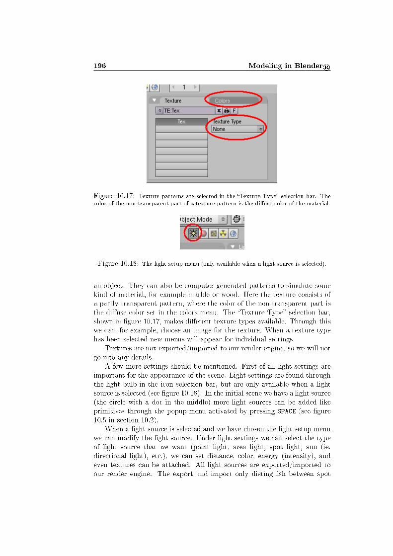
196 Modeling in Blender r

Figure 10.17: Texture patterns are sele ted in the �Texture Type� sele tion bar. The olor of the non-transparent part of a texture pattern is the di�use olor of the material. Figure 10.18: The light setup menu (only available when a light sour e is sele ted).an obje t. They an also be omputer generated patterns to simulate somekind of material, for example marble or wood. Here the texture onsists ofa partly transparent pattern, where the olor of the non-transparent part isthe di�use olor set in the olors menu. The �Texture Type� sele tion bar,shown in �gure 10.17, makes di�erent texture types available. Through thiswe an, for example, hoose an image for the texture. When a texture typehas been sele ted new menus will appear for individual settings.Textures are not exported/imported to our render engine, so we will notgo into any details.A few more settings should be mentioned. First of all light settings areimportant for the appearan e of the s ene. Light settings are found throughthe light bulb in the i on sele tion bar, but are only available when a lightsour e is sele ted (see �gure 10.18). In the initial s ene we have a light sour e(the ir le with a dot in the middle) more light sour es an be added likeprimitives through the popup menu a tivated by pressing SPACE (see �gure10.5 in se tion 10.2).When a light sour e is sele ted and we have hosen the light setup menuwe an modify the light sour e. Under light settings we an sele t the typeof light sour e that we want (point light, area light, spot light, sun (ie.dire tional light), et .), we an set distan e, olor, energy (intensity), andeven textures an be atta hed. All light sour es are exported/imported toour render engine. The export and import only distinguish between spot

10.3 Material Settings in Blender 197 Figure 10.19: Ba kground is set in the world settings menu. Figure 10.20: Render menu i on.lights and point lights, the rest will be exported as the one of these that best�t. The ba kground of our rendered image an be set in the world settings hosen by the i on whi h is a globe (�gure 10.19). World settings are sim-ply settings for the ba kground, whi h an be set to anything from a skysimulation to a single olor or an image. The ba kground settings are notexported.The last button in the i on menu bar is radiosity settings, whi h are notused in this proje t.To see the results from our modeling e�orts we turn to the renderingmenus. These are found in the stationary i on sele tion bar (the one that isalways visible). The render menus are sele ted through the small lands apei on (�gure 10.20).When pressing the big render button in the middle of the render menuwindow (also seen in �g. 10.1), Blender will generate a pi ture from the urrent amera view. Di�erent settings an be toggled on and o�, su h asshadows, ray tra ing, radiosity, et . The output pi ture is shown immedi-ately after al ulation has been arried out in a popup menu. The size andformat of the output pi ture is set in the rightmost menu alled format. Therendering image an be saved by pressing F3. The rendering fun tionalityis good for previews of the s ene. As it is now, it is hard to use the ren-der output for omparisons with the results of our render engine, sin e theexport/import s ripts hange too many things with regards to material andlight settings.After setting materials, we an start animating the s ene. Blender ani-mation is the subje t of the next se tion.

198 Modeling in Blender r Figure 10.21: The frame ounter.10.4 Blender AnimationTo reate a dynami s ene we an animate our obje ts. The basi animation on epts are des ribed in hapter 9, this se tion will follow hapter 9 anddes ribe how animation is arried out in Blender.Obje ts an be animated in Blender using key frames. The frame ounteris found in the lower menu bar, see �gure 10.21.Before reating any key frames it is a good idea to bring up the keyviewer. For this purpose we split the modeling view in two (as des ribed inse tion 10.1, right- li k on the edge of the window and sele t split). We wantto make one of our windows a key viewer, to do this; go to the window typesele tion i on in the lower left orner of the window and sele t the �NLAEditor� (see �gure 10.22).To make the �rst key frame go to the modeling view and sele t the obje tthat should be animated. When the obje t is pla ed in its �rst position, westart applying transformations and rotations by pressing CTRL+AKEY followedby �Ok�. Now we are ready to reate our �rst key frame. This is doneby pressing the IKEY and sele ting �Lo RotSize� to save position size androtation of the obje t. A small yellow box will now appear on a line for thesele ted obje t in frame one. This indi ates that a key frame has been saved,See �gure 10.23.Now, move the frame ounter to the frame where the next key frameshould be. In this frame hange the obje t to the next position, press IKEYand save another key frame. Moving through the di�erent frames it is seenthat the obje t will hange transformation between the two key frames. Tomake the animation longer or more detailed save more key frames in-betweenthe other frames. Key frames an be moved about, deleted, and sele ted inthe NLA editor exa tly as in the modeling view. Zoom fun tionalities analso help reating a better overview of the key frames, these works in thesame way as in modeling (see se tion 10.1). To stret h the view in onedire tion hold down CTRL+MMB and drag the mouse, either horizontally (xdire tion) or verti ally (y dire tion).The ourse of the transformation between the two key frames an be hanged in the �Ipo Curve Editor� found in the window type sele tion menujust like the �NLA Editor� (see �gure 10.22). The Ipo urve editor shows

10.4 Blender Animation 199

Figure 10.22: Sele t the �NLA Editor� to get an overview of the generated key frames.

Figure 10.23: Saving a key frame by pressing the IKEY. Here a key frame is saved for a ylinder.

200 Modeling in Blender r a urve for ea h transformation of the sele ted obje t. As we have savedkeys for lo ation, rotation, and s aling we have a urve for ea h of thesetransformation types on ea h axis (a total of nine urves). Figure 10.24shows how the Ipo urve editor looks like in our ase.The urve overview may be a bit onfusing sin e many urves sometimes ross ea h other. To on entrate at one transformation at the time, we an li k di�erent urves on and o� to the right using the Blender sele tion anddesele tion fun tionalities. To sele t a urve press the text and not on the olored square in front of the text. Pressing the olored square sele ts the urve instead. When a urve is sele ted we an transform it as we transformobje ts in the modeling view. To hange the form of the urve press TAB. Itis now possible to alter single points on the urve and the urve slope.As presented in hapter 9 we an reate an armature for more omplexmeshes. To reate an armature press SPACE, then sele t �Add� and thensele t �Armature� (see �gure 10.25).When you drag the mouse a bone will appear drawn from the �rst pointindi ating the beginning of this bone hain. Ea h time LMB is pressed onebone ends and a new bone begins. The bones are linked together in a hain.Around ea h link point we an move the armature freely; otherwise it hasonly sti� lines of onne tion. The links of the armature an be translated asother verti es in the modeling view. A bone is sele ted by sele tion of thetwo links that it is onne ting. Bones an be rotated and s aled. A typi alarmature for a human is shown in �gure 10.26.Sometimes it is appropriate to onne t links without a tually having abone between them (these are the dotted lines in �gure 10.26), this is doneby parenting. To make one bone parent of another, we must be in edit mode(Blender automati ally hanges to edit mode when we hoose to add anarmature). In the edit menu sele ted through the quad in the i on menu bar(see �gure 10.4 in se tion 10.1) we an set the parent of all sele ted bones.When a bone is made hild of another bone it will automati ally follow hanges of that bone. Figure 10.27 shows the parenting of the armature in�gure 10.26. Noti e that the pelvis is not a hild of any other bone, thismeans that when we move the pelvis the rest of the armature will followwithout transforming.The names of the bones are quite important in the parenting pro ess.The name of a bone is set in the BO �eld by LMB li king, exa tly as whennaming obje ts, materials, and textures. To name the bones it is a goodidea to sele t them one by one, only sele ted bones appear in the armaturebones menu.When the armature is done it should be �tted to the obje t that youwant to use it for. Think of the armature as the skeleton of the obje t. Alsotry to keep the enter of the armature in the same pla e as the enter of themesh, the enter is best pla ed between the feet lose to the ground (this isthe enter of rotation of the entire mesh a.k.a. the pelvis).

10.4 Blender Animation 201

Figure 10.24: The �Ipo Curve Editor�. Here we have saved key points for lo ation,rotation, and s aling of a ylinder in frame 1 and frame 20 (the view has been hangedusing zoom and stret h fun tionalities). The verti al green line indi ates the urrent frameshown in the modeling view.

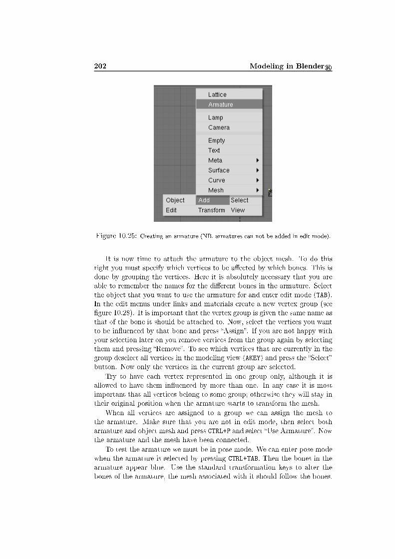
202 Modeling in Blender r

Figure 10.25: Creating an armature (NB. armatures an not be added in edit mode).It is now time to atta h the armature to the obje t mesh. To do thisright you must spe ify whi h verti es to be a�e ted by whi h bones. This isdone by grouping the verti es. Here it is absolutely ne essary that you areable to remember the names for the di�erent bones in the armature. Sele tthe obje t that you want to use the armature for and enter edit mode (TAB).In the edit menus under links and materials reate a new vertex group (see�gure 10.28). It is important that the vertex group is given the same name asthat of the bone it should be atta hed to. Now, sele t the verti es you wantto be in�uen ed by that bone and press �Assign�. If you are not happy withyour sele tion later on you remove verti es from the group again by sele tingthem and pressing �Remove�. To see whi h verti es that are urrently in thegroup desele t all verti es in the modeling view (AKEY) and press the �Sele t�button. Now only the verti es in the urrent group are sele ted.Try to have ea h vertex represented in one group only, although it isallowed to have them in�uen ed by more than one. In any ase it is mostimportant that all verti es belong to some group; otherwise they will stay intheir original position when the armature starts to transform the mesh.When all verti es are assigned to a group we an assign the mesh tothe armature. Make sure that you are not in edit mode, then sele t botharmature and obje t mesh and press CTRL+P and sele t �Use Armature�. Nowthe armature and the mesh have been onne ted.To test the armature we must be in pose mode. We an enter pose modewhen the armature is sele ted by pressing CTRL+TAB. Then the bones in thearmature appear blue. Use the standard transformation keys to alter thebones of the armature, the mesh asso iated with it should follow the bones.

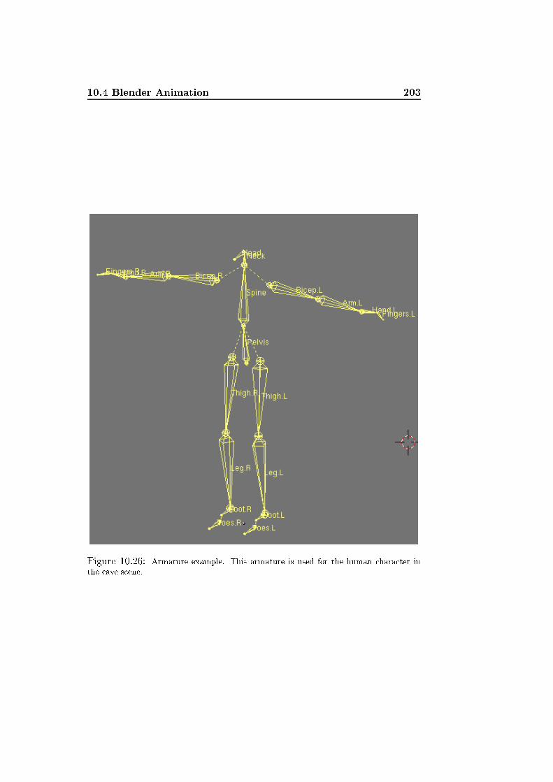
10.4 Blender Animation 203

Figure 10.26: Armature example. This armature is used for the human hara ter inthe ave s ene.

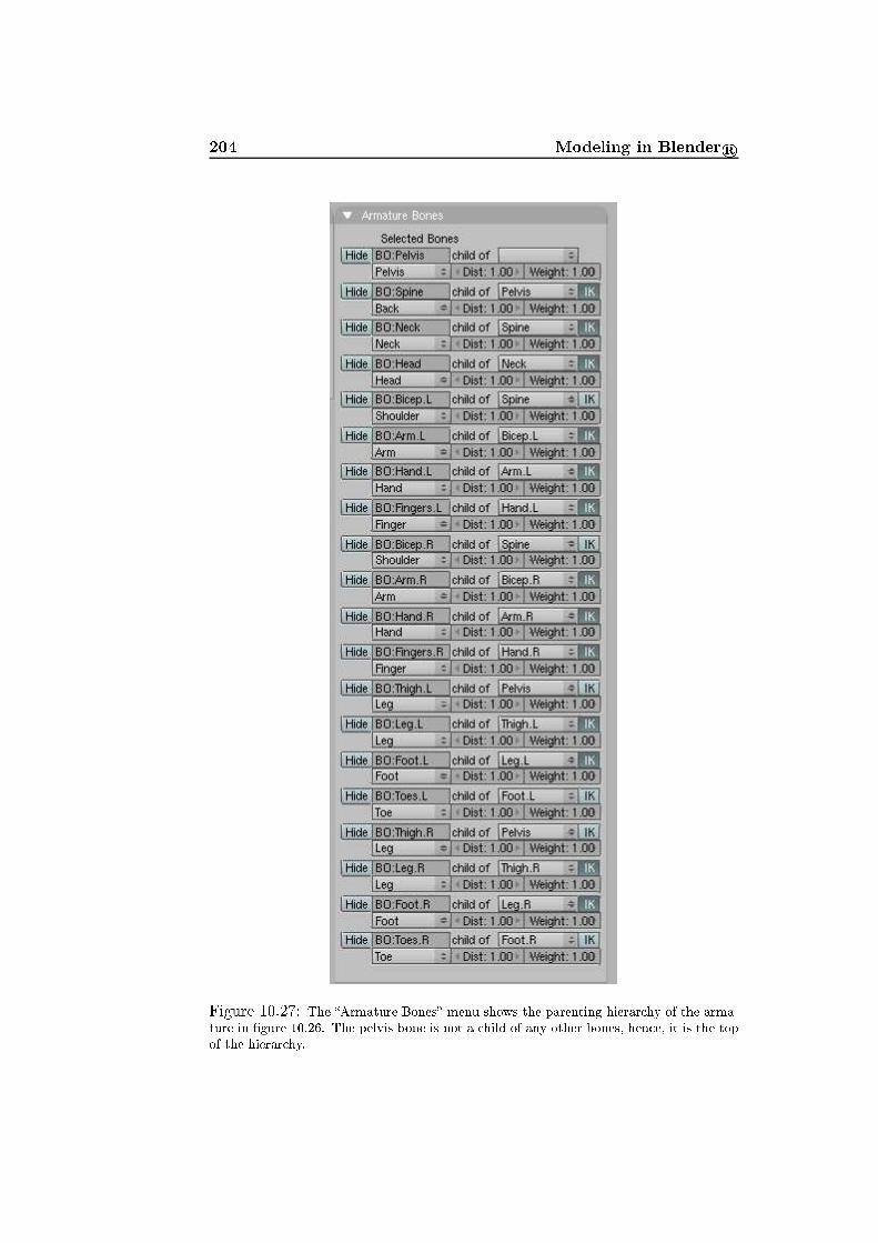
204 Modeling in Blender r

Figure 10.27: The �Armature Bones� menu shows the parenting hierar hy of the arma-ture in �gure 10.26. The pelvis bone is not a hild of any other bones, hen e, it is the topof the hierar hy.

10.4 Blender Animation 205

Figure 10.28: Creating a vertex group. The name of the group must be the same asthe bone that should in�uen e it. In this menu verti es are assigned, removed, sele ted,and desele ted from the urrent vertex group as well.Some ommon errors are: Verti es not hanging position with the armaturebe ause they do not belong to any group, and verti es from strange pla es inthe mesh that respond to transformations of the wrong bones be ause theyare assigned to a wrong group. Su h errors only reveal them selves by testingthe armature in pose mode.At all times, in pose mode, it is possible to lear transformations and re-turn the mesh and armature to the their starting positions by pressing ALT+R,ALT+S, and ALT+G to lear rotation, s aling, and translation respe tively.As with animation des ribed earlier in this se tion, we an save keyframes for the armature. The only di�eren e is that we are now saving a -tions, so instead of the �NLA Editor� we use the �A tion Editor�, see �gure10.29.In the a tion editor we see the same yellow boxes representing key frames,there is a key frame for ea h bone in the armature though (the armature mustbe sele ted to show any key frames in the a tion editor).In games we often make use of animation y les that an be used insequen es. Cy les are done most easily by opying the key frames fromframe one to the last frame in the y le and then �ll the spa e in-betweenwith other key frames. In this way we are sure to reate a y le. It is possibleto have many di�erent y les in blender. To begin a new y le sele t �AddNew� in the lower menu bar of the a tion editor view (see �gure 10.30).To view animations turn to the render menus (the small lands ape i onin the i on sele tion bar, see �gure 10.20 in se tion 10.3). Instead of the�Render� menu use the �Anim� menu. Set the number of frames to the samenumber of frames used in the y le and press �ANIM�. Blender now rendersall the frames needed to play the animation. When all frames have beenrendered press �PLAY� to view the animation. The animation will appearin a popup window and replay until the window is losed. Figure 10.31

206 Modeling in Blender r

Figure 10.29: Sele ting the �A tion Editor� to view key a tions instead of key transfor-mations.

Figure 10.30: Multiple y les an be reated. To begin a new y le sele t �Add New�in the lower menu bar of the a tion editor view.

10.5 Export S ripts and Import Libraries 207

Figure 10.31: The �Anim� menu.demonstrates the �Anim� menu.The next se tion des ribes the options we have when we want to exportour blender models and import them to our own renderer.10.5 Export S ripts and Import LibrariesAll data in Blender an be a essed via a Blender Python interfa e. Python1is an interpreted obje t-oriented programming language suitable for s riptingamong other things. As any other tool used for this proje t (ex ept for MSWindows) Python is freeware.To render the s enes reated in Blender with our own render engine, wemust export them to a �le format that an subsequently be imported in ourown appli ation. The simplest way is to export all data to a �le de�ninga C++ fun tion, whi h initializes all the data dire tly to our renderer at ompile time. The export s ript we wrote for this purpose is simply alledexport.py, sour e ode is available on the atta hed CD-ROM, see appendixA. In order to run su h an export s ript in Blender �rst split the modelingview (see �gure 10.3, se tion 10.1). Press SHIFT+F11 over one of the newwindows to swit h to text editor mode (or hoose �Text Editor� in the windowtype menu, see eg. �gure 10.29), then press ALT+SHIFT+FKEY while the mouseis over the text editor and hoose �Open...� in the popup menu (see �gure10.32). Browse to �nd export.py and open it in the text editor.The �rst line of the export s ript is FILENAME = "path", where path isthe full path of some . pp �le name. Set the path and �le name as you see�t. The hosen �le will be the resulting export. Now, simple press ALT+PKEY1URL: http://www.python.org/

208 Modeling in Blender r Figure 10.32: Opening a s ript �le.while the mouse is over the text editor. Some info will be printed to the onsole window Blender always keeps open beside the main window. The. pp �le given as path will then ontain a . pp �le initializing a world forour rendering appli ation.The ode export works well for small s enes and it's a good way to getstarted. However, when the s enes in rease in size, the ompile time of theexported ode es alates intolerably. It is there ne essary to use an inter-mediary �le format. Blender supports export to di�erent formats (under�le!export), but we have hosen to use an XML (eXtensible Markup Lan-guage) based �le format for 3D models alled X3D [143, 144℄. This easedthe work we had to do with respe t to import, sin e there exist open sour etools for parsing of XML, and besides an X3D importer written by BentDalgaard Larsen was distributed in the DTU ourse �Computer Graphi s�(02501). This importer is alled BMesh and it makes use of the open sour eC library for XML parsing alled Expat, written by James Clark2.A s ript for exports from Blender to X3D also exists, it is written byAdrian Cheater and the s ript �le is alled x3d_export.py3. The s ript is,however, at the development stage (June 12, 2004 - version 0.16). Never-theless it presented a ni e framework, whi h we have modi�ed and mademore robust for this proje t. To export a Blender s ene or part of a s enewith x3d_export.py follow the same steps as above until the s ript has beenopened. No path need to be set in this export s ript. Instead when ALT+PKEYis pressed the popup menu shown in �gure 10.33 will appear.After hoosing whether to export the entire s ene or only sele ted obje ts,the Python s ript will query the �le name of the export. Beware that thisexport s ript only works properly if you are using Blender 2.32 or newer,and if you have Python 2.3 or newer installed. It should also be noted thatbe ause of the early development stage of the s ript errors may easily o urand limitations to the export exist.The import alled BMesh is also a frame work at an early developmentstage. Therefore the import has many de� ien ies. On the other hand the ode is `friendly' and allows expansions without ausing too many troubles.For this reason we have been able to onne t the BMesh import to our render2URL: http://www.libexpat.org/3URL: http://www.bitbu ket. a/�a heater/blender/

10.6 Additional Blender Features 209

Figure 10.33: Exporting Blender models to X3D.engine. Still there is room for many optimizations in the export/import partof this proje t.One example of an export/import short oming is that the import supporttextures, while the export does not provide the ne essary texture images.Another example is that normals are exported, but not imported by theBMesh. Instead they are re- al ulated in some way that does not alwaysgenerate better results.Though we ould have made many other hoi es with respe t to exportand import, we hose those options that gave us as mu h freedom as possiblewith respe t to hanges in the implementation. In return we had to opewith some of the limitations that naturally follows with programs at an earlydevelopment stage.Here ends out dis ussion on export s ripts and import libraries. The nextse tion on ludes this hapter by mentioning some of the Blender featuresthat have otherwise not been des ribed in this hapter.10.6 Additional Blender FeaturesThe fun tionalities that have been des ribed in this hapter onstitute only asubset of Blender's apabilities. We have mainly des ribed the fun tionalitiesthat have been used to reate test s enes for this proje t, and s enes that wehad hoped to use as test s enes.Blender is ontinuously developing, and as far as we are on erned onlyfor the better. This hapter builds on version 2.33, when we started theproje t the newest version was 2.32 and already version 2.34 is available atblender.org. Fortunately fun tionalities are fairly ompatible between theversions and mu h is done to des ribe the new features that newer versionspresent. Manuals and tutorials for older versions are also still available for

210 Modeling in Blender r download, and sin e Blender is free of harge many amateurs write tutorialswhi h they make available on the net.The most extensive extra feature for Blender not mentioned until nowis the build in game engine. It is a tually possible to reate your own 3Dgame using Blender only. The game engine provides a physi al engine and anumber of fun tion alls to reate a game from a s ene. A good des riptionof how to reate games in Blender is found in [113℄. Of ourse informationabout this an be found on the internet too.Sin e all data are available through the Python interfa e to Blender,fairly omplex games an be reated through the ombination of Blenderand Python s ripting. The Python interfa e also gives the game engine anextra dimension with respe t to export of features to other appli ations.Python has a ess to the main loop of the game engine and an, therefore,a ess game parameters su h as transformations and physi al for es on the�y. These an be re orded as a kind of physi s dependant key frames, in thisway the Blender game engine an be used to reate intera tive animationsequen es very qui kly. Afterwards they an be exported and tested on anexternal renderer su h as the one written for this proje t.All in all we think that the ombination of Blender and Python is apowerful tool, whi h is quite useful for modeling and animation of test s enesfor external renderers. Blender is another step towards a game developmentplatform whi h is free of harge. That ends the part of this proje t that on erns modeling of ontents for 3D rendering.

Part IIIIdeas, Results, andExperiments

213The pre eding hapters have presented little new ex ept for the idea of anarray based math engine (se . 2.1), and few experiments apart from theexpanded tra k ball (se . 9.3) and the model-to- ode export s ript (se . 10.5).Yet we �nd that the theory given in part I is indispensable when we want todes ribe our own ideas, how they ame to us, and why we dis arded them orheld on to them. The more pra ti ally oriented part II is a ne essity for us inorder to show the possibilities of a free of harge game development platform,and part II is important in order to supply our report with anything moreinteresting than a stati standard s ene (su h as a still image of a Cornellbox).In other words the two previous parts provide the foundation from whereideas emerge and experiments ome into mind. Building on this, we willnow fo us on the ideas that have appeared during the proje t. The mainidea has be ome the Dire t Radian e Mapping (DRM) method whi h wehave referred to from time to time throughout the report and whi h will bedes ribe in detail. Other ideas will also be presented and dis ussed, somehave been implemented too. Dire t Radian e Mapping was, however, theidea that we hose for further development towards the end of the proje t.Chapter 11 will present the ideas that we have ome up with during theproje t. We will dis uss possibilities and drawba ks for ea h of them. Thiswill often lead to the reason why we hose not to bring the idea any further inthis proje t. A few ideas have been implemented on an experimental stage,in these ases the results will be dis ussed as well.Going through the proje t idea by idea eventually leads to the on eptthat we have hosen to sti k by: A method we have named Dire t Radian eMapping (DRM). The method builds upon basal radian e al ulations and ontains few restri tions and pre onditions. DRM is based on the newestGPU te hnology, and the method will draw advantage when GPUs growfaster and more e� ient. This means that the method may stand evenstronger in the future. First of all we use DRM to al ulate indire t illu-mination, but there are other appli abilities that will be tried out as well,an example is subsurfa e s attering. Chapter 12 will des ribe the method indetail.DRM is mainly a method for simulation of indire t illumination, and assu h it an easily be ombined with other methods addressing di�erent partsof the rendering equation (see hap. 6). Chapter 13 will mention all the ad-ditional methods that we have implemented for ombination with DRM. Wewill also mention implemented methods that are not for real-time rendering.Those have mainly been implemented for omparison. The radiosity im-plementation was originally implemented as an exer ise in the DTU ourse�Computer Graphi s� (02561), therefore it does not use the same renderengine as the rest of the rendering methods in our appli ation. Still a radios-ity implementation is very useful for omparison, and it has therefore beenbrought along and given a menu of its own in our viewer.

214Apart from DRM we have put an e�ort in onstru tion of a graphi al userinterfa e (GUI) alled JR Viewer, whi h shows how the global illuminatione�e ts that we are reating works in real-time ompared to standard globalillumination rendering (based on hap. 4). We have implemented a ray tra eras well as a radiosity renderer apable of rendering some prede�ned s enes(Cornell box ontaining a few obje ts). These s enes an also be renderedusing our di�erent real-time global illumination e�e ts. If our method wasto be used in a more extensive real-time 3D environment, we would need tobe able to render more omplex s enes than a Cornell box. As a part of theproje t we have taught ourselves how to model in Blender (see hap. 10) andwe have reated a � ave s ene� for testing our method. This s ene is alsoavailable in the GUI. Chapter 14 will des ribe the apabilities of the GUIand what we wish to show with our di�erent test s enes. Note that the GUIis a MS Windows appli ation and, hen e, does not run under other operatingsystems (Linux, Ma , et .). This was a hoi e we made in order to havesome extra windows features at our disposal (su h as drop down menus).Even though we have hosen not to emphasize on the pro ess of softwaredevelopment, rather on the appli ation of mathemati al tools to solve a omplex problem, implementation is inevitably a major part of the workthat must be done if we want to experiment or if we want to verify the ideasthat we put forth.Chapter 15 will present all the di�erent program parts and dis uss theirstru ture. All parts are bound together in our graphi al user interfa e, whi htherefore an be seen as the main part. From this part bran hes like raytra ing, radiosity and rasterization emerges. These are, on the other hand,all just di�erent ways of rendering the same s ene, therefore we will see thatmost of the rendering methods make use of the same render engine, whi his the ore of the appli ation.

Chapter 11Ideas

The best way to have a good idea is to have lots of ideas.Randall Jarrell: Pi tures from an institution (pt. 1, h. 4)

216 IdeasThe starting point of this proje t was to reate a de ent global illuminationrenderer and a simple real-time renderer. The implementation of those isdes ribed in hapter 15. Then the plan was to move them towards ea hother little by little and see if we ould make them meet midway.Our hoi e of global illumination algorithm was ray tra ing expanded byphoton mapping. This seemed to be the most general global illuminationmethod having a eptable performan e with respe t to pro essing time, the hoi e was, of ourse, also inspired by those who had previously been ableto simulate photon mapping in real-time or at intera tive rates, see se tion6.7.The �rst step was then to �nd optimization strategies for photon map-ping whi h ould lead it in a dire tion towards rasterization methods. Itsprings to mind when dealing with photon mapping that most of the timespend in the photon mapping algorithm is spend for ray tra ing. Ray tra ingis well explored with respe t to e� ien y and optimization s hemes, never-theless we had a few ideas for ray tra ing optimizations some of whi h werebased on graphi s hardware. Some of the ideas for ray tra ing optimizationsdeveloped into possible solutions for the entire global illumination problem.Others (those based on graphi s hardware) brought ray tra ing loser torasterization. The di�erent ideas are introdu ed in the following order:1. Angular visibility between axis aligned bounding boxes (AABBs) forfewer interse tion tests in ray tra ing.2. A topologi al network for radian e transfer between obje ts.3. Displa ement mapping for fast ray/obje t interse tion.4. A multi-agent approa h to global illumination, where ea h obje t is anautonomous agent ontrolling its own shade.5. An `atmosphere' to limit the in�uen e of ea h obje t in global illumi-nation.6. A line-of-sight algorithm for fewer interse tion tests in ray tra ing.7. Gouraud interpolation of the �rst interse tion point. A rasterizationapproa h to the �rst level of the ray tra ing algorithm.8. Single pixel images ea h representing a ray. An attempt to let rasteri-zation do full re ursive ray tra ing.Keep in mind that these se tions merely introdu e the ideas. Some ofthem have not been implemented, but are presented here to give an insightin the pro ess it was to �nd the �nal idea, and they give a feel of the hoi eswe had to make before starting to pursue a spe i� idea. Our �nal idea ofdire t radian e mapping emerged when we started at the other end of the

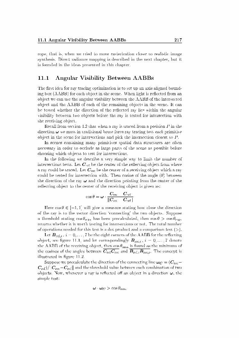
11.1 Angular Visibility Between AABBs 217rope, that is, when we tried to move rasterization loser to realisti imagesynthesis. Dire t radian e mapping is des ribed in the next hapter, but itis founded in the ideas presented in this hapter.11.1 Angular Visibility Between AABBsThe �rst idea for ray tra ing optimization is to set up an axis aligned bound-ing box (AABB) for ea h obje t in the s ene. When light is re�e ted from anobje t we an use the angular visibility between the AABB of the interse tedobje t and the AABB of ea h of the remaining obje ts in the s ene. It anbe tested whether the dire tion of the re�e ted ray lies within the angularvisibility between two obje ts before the ray is tested for interse tion withthe re eiving obje t.Re all from se tion 4.2 that when a ray is tra ed from a position P in thedire tion ! we must in traditional brute for e ray tra ing test ea h primitiveobje t in the s ene for interse tions and pi k the interse tion losest to P .In s enes ontaining many primitives spatial data stru tures are oftenne essary in order to o lude as large parts of the s ene as possible before hoosing whi h obje ts to test for interse tions.In the following we des ribe a very simple way to limit the number ofinterse tions tests. Let Cref be the enter of the re�e ting obje t from wherea ray ould be tra ed. Let Cre be the enter of a re eiving obje t whi h a ray ould be tested for interse tion with. Then osine of the angle (�) betweenthe dire tion of the ray ! and the dire tion pointing from the enter of there�e ting obje t to the enter of the re eiving obje t is given as: os � = ! � Cre �CrefkCre �CrefkHere os � 2 [�1; 1℄ will give a measure stating how lose the dire tionof the ray is to the ve tor dire tion ` onne ting' the two obje ts. Supposea threshold stating os �max has been pre al ulated, then os � > os �maxreturns whether it is worth testing for interse tions or not. The total numberof operations needed for this test is a dot produ t and a omparison test (>).LetBref;i ; i = 0; : : : ; 7 be the eight orners of the AABB for the re�e tingobje t, see �gure 11.1, and let orrespondingly Bre ;i ; i = 0; : : : ; 7 denotethe AABB of the re eiving obje t, then os �max is found as the minimum ofthe osines of the angles between CrefCre and Bref;iBre ;i. The on ept isillustrated in �gure 11.2.Suppose we pre al ulate the dire tion of the onne ting line !C = (Cre �Cref)=kCre �Crefk and the threshold value between ea h ombination of twoobje ts. Now, whenever a ray is re�e ted o� an obje t in a dire tion !, thesimple test: ! � !C > os �max

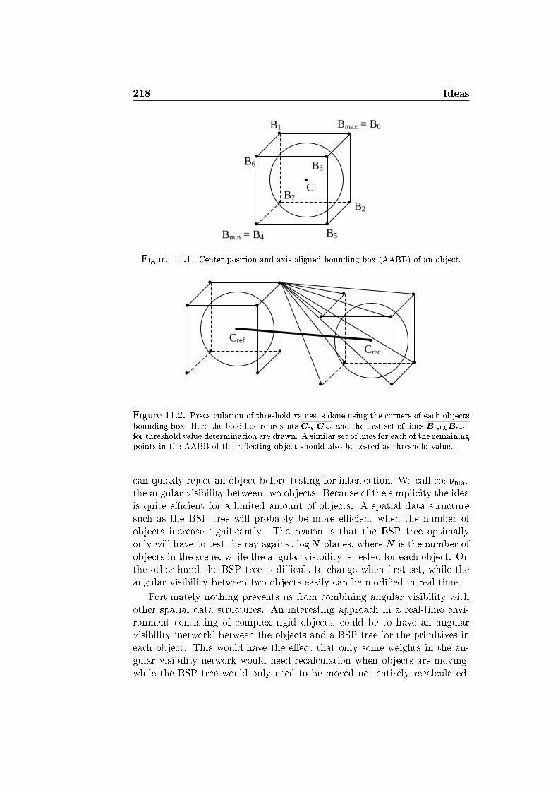
218 Ideas

Bmin = B4

Bmax = B0

B5

B1

B3 B6

B2 B7

•

•

•

• •

•

•

•

• C

Figure 11.1: Center position and axis aligned bounding box (AABB) of an obje t.

•

•

•

• •

•

•

•

• Cref

•

•

•

• •

•

•

•

• Crec

Figure 11.2: Pre al ulation of threshold values is done using the orners of ea h obje tsbounding box. Here the bold line represents CrefCre and the �rst set of lines Bref;0Bre ;ifor threshold value determination are drawn. A similar set of lines for ea h of the remainingpoints in the AABB of the re�e ting obje t should also be tested as threshold value. an qui kly reje t an obje t before testing for interse tion. We all os �maxthe angular visibility between two obje ts. Be ause of the simpli ity the ideais quite e� ient for a limited amount of obje ts. A spatial data stru turesu h as the BSP tree will probably be more e� ient when the number ofobje ts in rease signi� antly. The reason is that the BSP tree optimallyonly will have to test the ray against logN planes, where N is the number ofobje ts in the s ene, while the angular visibility is tested for ea h obje t. Onthe other hand the BSP tree is di� ult to hange when �rst set, while theangular visibility between two obje ts easily an be modi�ed in real-time.Fortunately nothing prevents us from ombining angular visibility withother spatial data stru tures. An interesting approa h in a real-time envi-ronment onsisting of omplex rigid obje ts, ould be to have an angularvisibility `network' between the obje ts and a BSP tree for the primitives inea h obje t. This would have the e�e t that only some weights in the an-gular visibility network would need re al ulation when obje ts are moving,while the BSP tree would only need to be moved not entirely re al ulated,

11.1 Angular Visibility Between AABBs 219sin e the obje ts were assumed to be rigid.This was the �rst idea. The angular visibility network has been imple-mented, unfortunately we have not had the time to ombine it with a BSPtree. The results of an angular visibility network are good in the simple Cor-nell box s ene whi h is otherwise often too simple to bene�t from spatial datastru tures. Improvements due to angular visibility tests alone are roughly26% when ray tra ing a Cornell box with a hrome (or mirror) sphere and aglass sphere (12 triangles and 2 spheres) in luding spe ular re ursions, hardshadows, and phong shading. The resulting image is shown in �gure 11.3.

Figure 11.3: A Cornell box with a hrome (or mirror) sphere and a glass sphere (12triangles and 2 spheres). The s ene was used as a test of the e� ien y of the angularvisibility network. The spe i� render in ludes spe ular re ursions, hard shadows, andphong shadingThere is room for further improvements on the method. If an AABB ontains a triangle only, it would, in fa t, be mu h more e� ient to �nd theangular visibility using the orners of the triangle instead of the orners ofthe bounding box.The idea of an angular visibility network is interesting sin e the angularvisibility ould be a measure of the amount of energy whi h should be trans-ferred between two obje ts. This idea is explored a little further in the nextse tion.

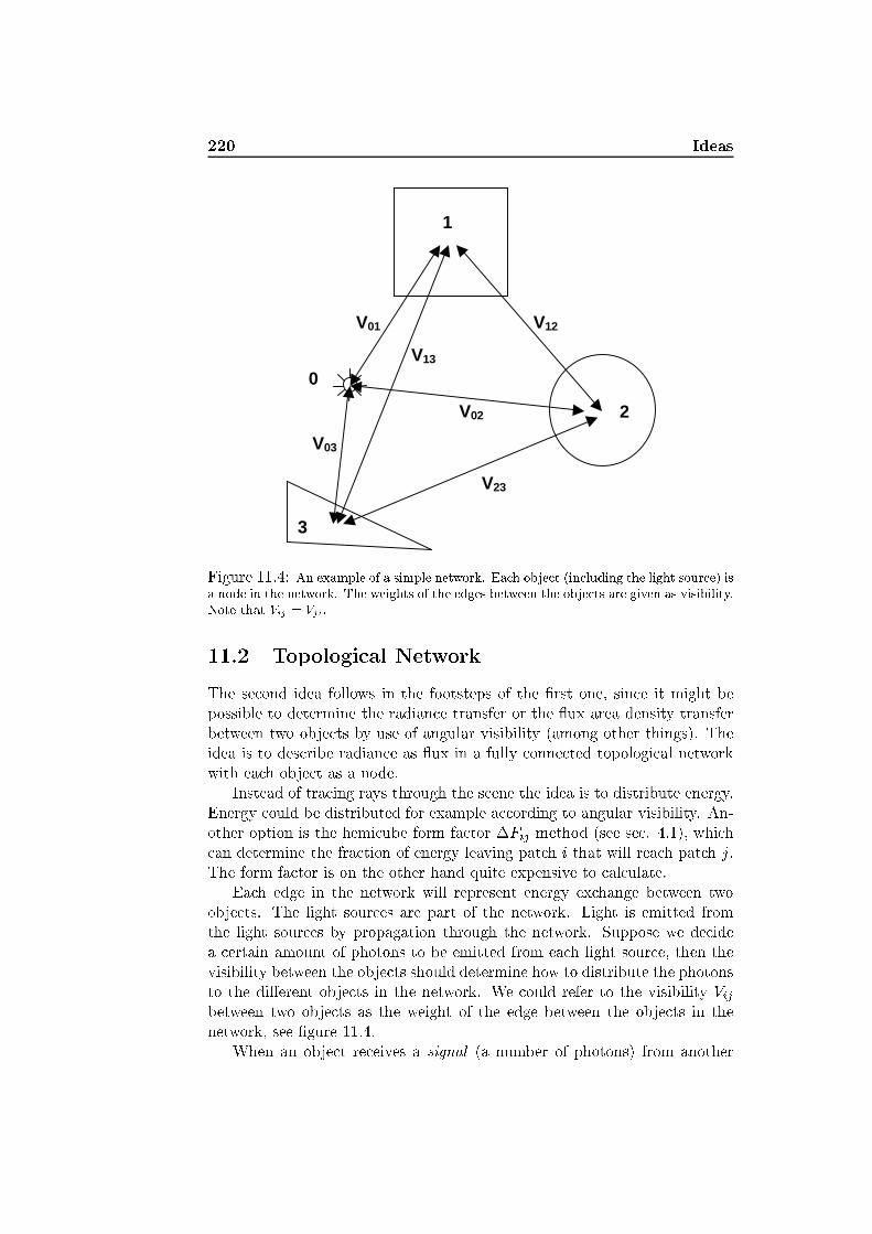
220 Ideas

1

2

3

0

V01

V13

V03

V12

V23

V02

Figure 11.4: An example of a simple network. Ea h obje t (in luding the light sour e) isa node in the network. The weights of the edges between the obje ts are given as visibility.Note that Vij = Vji.11.2 Topologi al NetworkThe se ond idea follows in the footsteps of the �rst one, sin e it might bepossible to determine the radian e transfer or the �ux area density transferbetween two obje ts by use of angular visibility (among other things). Theidea is to des ribe radian e as �ux in a fully onne ted topologi al networkwith ea h obje t as a node.Instead of tra ing rays through the s ene the idea is to distribute energy.Energy ould be distributed for example a ording to angular visibility. An-other option is the hemi ube form fa tor �Fij method (see se . 4.1), whi h an determine the fra tion of energy leaving pat h i that will rea h pat h j.The form fa tor is on the other hand quite expensive to al ulate.Ea h edge in the network will represent energy ex hange between twoobje ts. The light sour es are part of the network. Light is emitted fromthe light sour es by propagation through the network. Suppose we de idea ertain amount of photons to be emitted from ea h light sour e, then thevisibility between the obje ts should determine how to distribute the photonsto the di�erent obje ts in the network. We ould refer to the visibility Vijbetween two obje ts as the weight of the edge between the obje ts in thenetwork, see �gure 11.4.When an obje t re eives a signal (a number of photons) from another

11.3 Displa ement Mapping 221obje t the photons are distributed over the area of the re eiving obje t whi his visible from the re�e ting (or emitting) obje t. Environment maps (seese . 6.3) ould be used to determine these areas.After emission and propagation in the network the temporary energy ofthe obje t de reases, while the temporary energy of the obje ts that havere eived photons in reases. Now, suppose we set some threshold for ea hobje t. When the temporary energy passes above the threshold, the obje tis marked for re�e tion of energy. In the next step of the algorithm all obje tsmarked for re�e tion will propagate energy ba k into the network, while stillstoring the photons they re eived. Now, the re ursion an ontinue until anequilibrium state is rea hed. At this point the �nal image has been rea hed.Inspiration for this method was found in the idea of wave expansionneural networks [67, 68, 71℄, for those familiar with the resear h area ofneural networks the analogy qui kly be omes apparent.Though the method seems lose to progressive re�nement as des ribedin radiosity, the di�eren e is that photons are distributed a ross the surfa eof an obje t. This means that we an let re�e ted energy originate in spe- i� photons in ident on an obje t and thereby photons propagated in thenetwork an have a spe i� dire tion and origin. This means that we anmodel arbitrary BRDFs if ne essary.The three main di� ulties in this method are visibility al ulations, re-�e tion (or refra tion) of light from an obje t to itself, and re on�gurationof the network when things hange dynami ally.To further expand the networking on ept ea h obje t ould itself ontaina network where sample lo ations a ross the surfa e would be nodes. In thisway the obje t would be able to intera t with itself. As suggested in [61℄ ina di�erent ontext, Turk's repulsion algorithm [127℄ ould be used to samplepoints a ross the obje t surfa e.Most of the on epts des ribed in this se tion are merely suggestions,nevertheless, the network analogy was also the origin of our dire t radian emapping idea (see hap. 12). If we do not hoose to have an internal networkfor ea h obje t, we ould instead distribute the in ident photons over thevisible part of the bounding box. The following se tion presents an ideafor pre al ulation of the interse tion test that must be al ulated when thephotons are tra ed from the bounding box to the exa t interse tion with there eiving obje t.11.3 Displa ement MappingComplex obje ts are often di� ult to ray tra e be ause they onsist of an im-mense number of triangles. Many methods exist to handle this problem, mostof them are based on spatial data stru tures. Spatial data stru tures spendtime �nding the right triangle for the interse tion al ulation. As an alter-

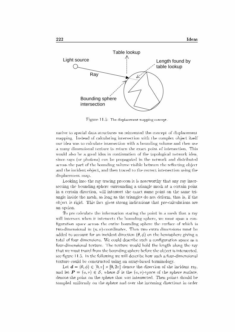
222 Ideas

Ray

Light source

Bounding sphere intersection

Table lookup

Length found by table lookup

Figure 11.5: The displa ement mapping on ept.native to spatial data stru tures we reinvented the on ept of displa ementmapping. Instead of al ulating interse tion with the omplex obje t itselfour idea was to al ulate interse tion with a bounding volume and then usea many dimensional texture to return the exa t point of interse tion. Thiswould also be a good idea in ontinuation of the topologi al network idea,sin e rays (or photons) an be propagated in the network and distributeda ross the part of the bounding volume visible between the re�e ting obje tand the in ident obje t, and then tra ed to the orre t interse tion using thedispla ement map.Looking into the ray tra ing pro ess it is noteworthy that any ray inter-se ting the bounding sphere surrounding a triangle mesh at a ertain pointin a ertain dire tion, will interse t the exa t same point on the same tri-angle inside the mesh, as long as the triangles do not deform, that is, if theobje t is rigid. This fa t gives strong indi ations that pre- al ulations arean option.To pre- al ulate the information stating the point in a mesh that a raywill interse t when it interse ts the bounding sphere, we must span a on-�guration spa e a ross the entire bounding sphere the surfa e of whi h istwo-dimensional in (u; v)- oordinates. Then two extra dimensions must beadded to a ount for an in ident dire tion (�; �) on the hemisphere giving atotal of four dimensions. We ould des ribe su h a on�guration spa e as afour-dimensional texture. The texture would hold the length along the raythat we must travel from the bounding sphere before the obje t is interse ted,see �gure 11.5. In the following we will des ribe how su h a four-dimensionaltexture ould be onstru ted using an array-based terminology.Let d = (�; �) 2 [0; �℄ � [0; 2�℄ denote the dire tion of the in ident ray,and let P = (u; v) 2 S, where S is the (u; v)-spa e of the sphere surfa e,denote the point on the sphere that was interse ted. Then points should besampled uniformly on the sphere and over the in oming dire tions in order

11.3 Displa ement Mapping 223to dis retize the axes. The stru tural operation behind a Cartesian produ t,that is, the array theoreti transformer alled OUTER (see de�nition 7), willthen span the entire on�guration spa e of the axes.De�nition 7 (OUTER) Let A1 and A2 be arrays of dataand let f be a binary �rst order fun tion, thenA1 OUTER f A2 (11.1)is de�ned as the fun tion f applied to all pairs de�ned by theCartesian produ t of the arrays A1 and A2.The dis retization of ea h �oating point axis will divide it into intervals.If we sample at midpoint of ea h interval, the on�guration spa e will holdthe midpoint of ea h ell in the four-dimensional texture. For ea h ellmidpoint we �nd the distan e to the point of interse tion by ray tra ing andassign to the texture value of that on�guration.We an now use a four-dimensional array (or texture) as a map M fromdire tion d of the in ident ray and position P of interse tion on the bound-ing sphere to distan e t that must be traversed along the ray before theinterse tion is found: M : [0; �℄� [0; 2�℄ � S ! Rwhere M 7! OUTER interse twhi h means that a sampling of the ontinuous spa e [0; �℄� [0; 2�℄� Sto dis rete axes and use of the stru tural operation behind an outer produ twith an interse tion algorithm, will span a on�guration spa e that leavest =M(d;P)being a simple table look-up. Having (of ourse) omplexity O(1).After re-inventing the on ept we found that it was already well exploredand known as view-dependent displa ement mapping, see [131℄. The abso-lute largest drawba k is the size of the array. On top of this the displa ementmap of a parti ular obje t would basi ally need re al ulation ea h time trans-formations other than translations or rotations are arried out. Translation an be done without re al ulation sin e the array on erns the bounding boxand the obje t, not the surroundings as su h. This is also true for rotationif the bounding volume is a sphere. (Uniform s aling may also be possiblesin e the lengths in the map an s ale a ordingly.)

224 IdeasThe idea of a table look-up for ray tra ing arries on to some of oursubsequent ideas. In the following se tion we turn to a more general on ept,whi h ould be applied in ombination with many other ideas.11.4 Multi-Agent Global IlluminationWith a ba kground in the area of arti� ial intelligen e, we qui kly ame upwith the idea of a multi-agent approa h to global illumination. The idea isto regard ea h obje t, be that in a topologi al network or not, as an agentwhi h must itself take are of its urrent shade at all positions a ross itssurfa e. This distributed approa h is interesting be ause of the parallelismthat is inherent in global illumination.Ea h obje t, whi h in this ontext is an autonomous agent, should runin its own program thread. Sensing is a well known on eption in multi-agent systems, a good referen e on multi-agent systems in general is [136℄.Whenever the obje t sense the surrounding it will update visibility of otherobje ts, for example by use of an environment map. The obje t will at anytime be able to re eive new pa kets of photons. They will, however, notbe pro essed until the agent thread is idle. The agent will also try to passon energy to those obje ts visible in its environment map. Ea h pa ket ofphotons will then be a message ontaining the information ne essary for there eiving agent to distribute the photons a ross its surfa e and again passon photons to visible obje ts.The advantages of a distributed approa h is that ea h obje t, in prin iple, an use di�erent rendering algorithms adapted spe i� ally for their nature.A very omplex obje t may get away with a simpler shading method andthereby not de rease the frame rate. An important aspe t of multi-agentsystems for dynami environments are anytime algorithms, meaning thatthe obje t must always have the best answer available at any time. In thisway the rendering an be made more robust. A single obje t may take along time to render but this will not stop the entire rendering pro ess, thatparti ular obje t will just update its shading a little too late (maybe every�fth frame).From our point of view the idea is indeed interesting, it seems to bringup many possibilities that have otherwise been unthought of. The problemis whether there is an overhead in the administration of a pseudo parallelthread for ea h obje t and the handling of the messages send between theagents. The idea of individually ontrolled obje ts is, however, appealingto us. The next se tion presents a simple idea whi h ould be useful, forexample in the ontext of a multi-agent system.

11.5 Obje t Atmosphere 225

Object A

Bounding sphere

Atmosphere

Influencing object B

Not influencing object C

Figure 11.6: Obje t A is in�uen ed by light re�e ted from obje t B, sin e this obje tinterferes with its atmosphere. Light from obje t C has no in�uen e, sin e this is outsidethe atmosphere of obje t A.11.5 Obje t AtmosphereNormally hanges in indire t illumination aused by other obje ts be omesinsigni� ant if the obje ts rea h a ertain distan e. A very simple idea, whi hlimits the amount of work that must be done, is to have a sphere of in�uen e,or an `atmosphere', around ea h obje t in order to limit the in�uential areaof obje ts in al ulations of indire t illumination, see �gure 11.6. The same on ept is known from light sour es, whi h often are supplied with a sphereof in�uen e. An obje t atmosphere ould be useful eg. for the multi-agentapproa h.This idea has not had mu h in�uen e on our urrent implementation.Another idea is to use a line of sight algorithm for ray tra ing optimization,this is the subje t of the following se tion.11.6 Line-of-Sight AlgorithmSuppose your s ene is divided into a regular grid (often only two-dimensional).Then the purpose of a line-of-sight algorithm is to �nd the exa t list of grid ells that a ray following the line of sight will pass through, see �gure 11.7. Ifwe use the line-of-sight algorithm for ray/obje t interse tion all empty grid ells will be thrown away. When a grid is rea hed ontaining obje ts thealgorithm will he k (if the algorithm uses a two-dimensional grid) whether

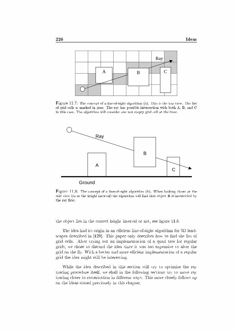
226 Ideas

A B C

Ray

Figure 11.7: The on ept of a line-of-sight algorithm (a). This is the top view. The listof grid ells is marked in gray. The ray has possible interse tion with both A, B, and Cin this ase. The algorithm will onsider one not empty grid ell at the time.

Ground

A C

B

Ray

Figure 11.8: The on ept of a line-of-sight algorithm (b). When looking loser at theside view (or at the height interval) the algorithm will �nd that obje t B is interse ted bythe ray �rst.the obje t lies in the orre t height interval or not, see �gure 11.8.The idea had its origin in an e� ient line-of-sight algorithm for 3D land-s apes des ribed in [129℄. This paper only des ribes how to �nd the list ofgrid ells. After trying out an implementation of a quad tree for regulargrids, we hose to dis ard the idea sin e it was too expensive to alter thegrid on the �y. With a better and more e� ient implementation of a regulargrid the idea might still be interesting.While the idea des ribed in this se tion still try to optimize the raytra ing pro edure itself, we shall in the following se tions try to move raytra ing loser to rasterization in di�erent ways. This more losely follows upon the ideas stated previously in this hapter.

11.7 First Interse tion in Hardware 22711.7 First Interse tion in HardwareThe �rst idea for moving ray tra ing loser to rasterization is to do the �rstlevel of ray tra ing in hardware. The idea is quite obvious be ause raster-ization an obtain images similar to ray tra ed images as long as spe ularre ursions are not in luded. In other words we may as well let the rasterizersolve the part of the rendering equation whi h simulates dire t illumination,while ray tra ing takes are of spe ular re ursions.The most important part of this idea is that we annot just render thedire t illumination as usual with the rasterizer. This would give us no im-provements with respe t to ray tra ing, sin e we would still need to startthe ray tra ing from the eye. What we need is to �nd the �rst interse tionpoints using the rasterizer. The pro edure is to make a simple vertex shaderthat s ales the position of ea h vertex (in world oordinates) to the interval[0; 1℄. This an be a omplished using an AABB of the s ene to be rendered.First give all primitive obje ts a spe i� olor id and draw the s ene (see�gure 11.9a), then draw the position of ea h fragment using Gouraud shadingand the simple vertex shader mentioned above (see �gure 11.9b). Those twoimages result in the �rst level of ray tra ing (interse tion point and id of theinterse ted triangle). From there on the ray tra ing an arry on as usual.For further optimization the depth bu�er ould be used to spe ify the t valueof the interse tion point for ea h ray (r = o+ td) that would eliminate thepass to make image b.

Figure 11.9: From left to right: (a) Color ids for ea h primitive in the s ene. (b) Positionof �rst interse tion s aled to the interval [0; 1℄.Another improvement is that shadow volumes an repla e shadow rays.The pro edure is for ea h light sour e to render the shadow volumes to thesten il bu�er as usual and then use the result to de ide whether light from aparti ular light sour e should ontribute to the shade of ea h ray representinga pixel.Using these improvements and the simple angular visibility idea des ribed

228 Ideasin se tion 11.1, traditional ray tra ing is improved as follows: Rendering�gure 11.10b takes 41% of the time we spend for the rendering of �gure11.10a. The slightly more omplex s ene of �gure 11.11 takes approximately26% of the referen e time. The rendering times are given in table 11.1.

Figure 11.10: Renderings of the Cornell box with two spheres. From left to right: (a)Referen e image using standard (one ray per pixel) ray tra ing. (b) The same imagerendered where the �rst interse tion was found in hardware.MethodnS ene Two spheres Orb on pedestalTraditional ray tra ing 10.297 s 137.547 sFirst interse tion in HW 4.218 s 36.125 sTable 11.1: Rendering times for the �rst interse tion in hardware improvement omparedto standard ray tra ing. Rendering was performed on a 1GHz Pentium 3 ma hine with aGeFor e4 MX440 SE.As seen in �gure 11.10, the ina ura y of the olor bu�er (8 bits per olor band) leads to some aliasing artifa ts lose to the lines and highlightsof re�e tions and refra tions. Using a fragment shader for the position imageor a pbu�er with higher pre ision may eliminate su h aliasing artifa ts.Opportunities for further improvements along the same line of thoughtare, for example, to do the BRDF al ulations in a fragment shader, or to�nd the the �rst re�e tion and refra tion ve tors for the re ursion to leveltwo in hardware using a simple vertex shader. We did not spend time forthese minor improvements sin e we hoped to �nd a more general approa h,whi h would be able to run in real-time.All the ideas des ribed in this se tion are useful for the �rst level ofray tra ing only. This means that highly spe ular s enes will not draw asigni� ant advantage from the method. The improvement is also relativeto how optimized the ray tra ing pro essing is with respe t to spatial datastru tures. A truly optimized ray tra er would bene�t less from doing the�rst step in hardware. Even if the improvements are not signi� ant the idea

11.8 Single Pixel Images 229

Figure 11.11: Rendering of the Cornell box with orb. A slightly more omplex s ene.Ambient light is in luded in this render, otherwise the pedestal under the orb wouldbe entirely bla k (traditional ray tra ing does not a ount for di�usely re�e ted indire tillumination).of a �rst step of ray tra ing fast enough for real-time is interesting and it willbe shown in hapter 12 how this an be exploited. Before the idea of dire tradian e mapping, our plan was to see if we ould do the entire ray tra ingpro ess using rasterization methods. Our brief approa h towards this end isdes ribed in the next se tion.11.8 Single Pixel ImagesAn experiment we did was to tra e the rays after the �rst level by movementof the amera and rendering of a size 1�1 image for ea h ray. The bottlene kis, of ourse, that ea h ray must travel all the way down the graphi s pipeline,whi h takes approximately half a millise ond on a GeFor e4 MX440 SE witha simple s ene su h as a Cornell box. This is hardly more e� ient thana highly optimized spatial data stru ture, but on the other hand no datastru ture need re onstru tion when obje ts start moving dynami ally.

230 IdeasThe idea would move the entire pro ess of ray tra ing to the GPU. How-ever, it is not very elegant. In fa t it utilizes the hardware in a ruel manner,sin e the entire s ene must be lipped for ea h ray that we want to tra e.If this approa h was to be a su ess, the GPUs would have to start empha-sizing on an ability to render a large amount low resolution images ratherthan an ability to pro ess an in reasing amount of fragments (high imageresolutions) and an in reasing amount of verti es (more triangles). Resultsfor single image pixels are not signi� antly better on a GeFor e 5950 and formore omplex s enes the render time for ea h single pixel image in reasessigni� antly. This indi ates that GPUs not likely will improve performan efor many low resolution images. We therefore qui kly realized that the ideahad little future.Many ideas have been mentioned in this hapter. Some more ompre-hensive than others. All of them originated in the movement from realisti image synthesis towards real-time rendering. None of them ame lose toreal-time performan e, at least none of those we had time to implement. Inthe following hapter we will in parti ular draw on the ideas of networking(se . 11.2) and �rst interse tion in hardware (se . 11.7) when we start witha real-time renderer and move towards global illumination.

Chapter 12Dire t Radian e Mapping

Assess the advantages in taking advi e, then stru ture your for esa ordingly, to supplement extraordinary ta ti s. For es are to bestru tured strategi ally, based on what is advantageous.Sun Tzu (�500 BC.): The Art of War

232 Dire t Radian e MappingAfter a presentation of several ideas whi h were either half pursued or halfdis arded, we will present the method that we hose to work with in parti -ular during the last part of our proje t. We have hosen to all the methodDire t Radian e Mapping (DRM) and to our knowledge no-one else havetried it out before. Therefore we regard DRM to be an important part ofour proje t.Re all the expansions of the rasterization approa h des ribed in hap-ter 6. As shown in that hapter one of the most signi� ant visual e�e ts,whi h is present in global illumination, but di� ult to model in real-time, islight re�e ted di�usely more than on e. Dire t radian e mapping is anothermethod for simulating multiple di�use re�e tions. Common for most meth-ods trying to solve this problem is that some limitations are in�i ted on thes ene dynami s. The general idea in our approa h is to apply as few limi-tations to the s ene dynami s as possible, and then always solve the simple ase before taking the next step towards full indire t illumination. This willespe ially be apparent in se tion 12.2.In se tion 12.1 we outline the basi ideas and sour es of inspiration behinddire t radian e mapping. Next, in se tion 12.2, the method is des ribed froma more pra ti al point of view and the progress of the method to its urrentstate is dis ussed. Abilities and limitations of dire t radian e mapping willbe dis ussed in se tion 12.3. In the �nal se tion of this hapter we will ompare dire t radian e mapping to the ompeting methods des ribed in hapter 6.12.1 The Con eptIn this se tion we will on entrate on the on eptual idea of dire t radi-an e mapping (DRM). What we des ribe here is an abstra t formulationwhi h shows the origin of DRM and its relation to the ideas mentioned inthe previous hapter. Our implementation does not ne essarily follow thisabstra t formulation, the next se tion will fo us on the resulting method forimplementation.The basi idea is to take a pi ture of the s ene from the point of view ofthe light sour e (as done in shadow mapping proposed by Lan e Williamsin [139℄), let this pi ture represent dire t illumination, then take a pi tureof the s ene from the eye point, representing visible points in the s ene. Bygoing through ea h point visible in the eye point pi ture and al ulating thelight ontribution from ea h point in the dire t illumination pi ture we getthe �rst boun e of indire t light. Figure 12.1 seeks to illustrate the pro ess.A more elaborate version of the on ept, whi h tells more about where it ame from and how it an open up further possibilities than a single boun eof indire t illumination, is explained in the following.Considering the rendering equation as a problem of wave propagation

12.1 The Con ept 233

Eye point Light source

Scene

Current point of interest

Figure 12.1: The basi idea of dire t radian e mapping. For ea h point of interest wemust al ulate the light ontribution from ea h dire tly illuminated point in the s ene.(in a similar way as propagation in the topologi al network was des ribedin se tion 11.2) we an split it into propagation of radian e from the lightsour es and propagation of importan e from the eye or the amera (re allthe on ept of importan e from se tion 3.6).The �rst step is then propagation of radian e from the light sour es. We ould denote this as follows: Li = PLe. In ident radian e is determinedby the point of interse tion, the in ident dire tion, and the in ident power.These information and, hen e, the entire �eld of dire t in ident radian e an be measured using images from ea h light sour e. The �rst point ofinterse tion an be found as des ribed in se tion 11.7. In ident dire tionsfollow from the position of the light sour e where an image is taken from.The dire t in ident power is given by the geometry term (G) between thelight sour e and the point of in iden e (visibility need not be onsidered,sin e everything seen from the light sour e will also be illuminated).The purpose of storing these information representing the in ident radi-an e �eld is not to estimate dire t illumination. Better methods exist forthat. Instead another image is taken this time from the eye point pi turingthe �rst step of importan e propagation. As with the radian e propagationimage the �rst points of interse tion are also stored for importan e propaga-tion. The in ident dire tions are given by the eye point and the importan eof the lo ations seen dire tly from the eye is always one (see (3.60)).The positions of dire t in ident radian e are now stored in a texture whi hwe might refer to as a dire t radian e map. It is quite similar to a photonmap sin e ea h texel ould be regarded as a photon. On the other hand itdoes not have a tree stru ture, and nor is it used for radian e estimates in the

234 Dire t Radian e Mappingsame way as a photon map is. The positions of dire t in ident importan eare stored in what we might refer to as a dire t importan e map. The texels ould in this ase be thought of as importons1. All in all we now have twomaps; one of dire t radian e and one of dire t importan e.To propagate the light waves further we need only onsider the lightthat by one way or another propagates to points of importan e. One wayto propagate waves is by means of random signals in a onne ted digraph(dire ted graph). If we let the edges of a graph, onne ting `importons' of thedire t importan e map with `photons' of the dire t radian e map, be given byan outer produ t, the result is a dire ted graph where ea h importon node isfully onne ted to all photon nodes (and oppositely ea h photon node will befully onne ted to all importon nodes). Random signals in su h a onne teddigraph would simulate the propagation of light if all importon nodes werefully visible to all photon nodes.To start out with the simple ase, we assume that all surfa e materialsare Lambertian. In that ase propagation of the signals an be performed ompletely at random, and we need merely gather radian e propagated fromrandom photon nodes towards random importon nodes and weigh the signalsby the normals. We even do not need to take the in ident dire tion into onsideration when signals are propagated in the network.The simple ase is too redu tive with respe t to photorealisti images.As always expansions ome at large expenses. First we ought to introdu e aBRDF at ea h photon node either sending signals towards ertain dire tionsor weighing signals a ording to in ident dire tion and material properties.This is a feasible task whi h enables the possibility of materials that are notperfe tly di�use (Lambertian).To model the indire t illumination properly, we should take the geometryin-between two nodes into a ount. This expansion from the simple aseis the most expensive and di� ult part of the global illumination problem.Visibility between two points ould be he ked in order to a ount for indire tshadows.Spe ular re�e tion and refra tion are also a part of the indire t illumina-tion, but te hniques su h as environment mapping an deal with these asesreasonably well, see se tion 6.3.The light propagation network is onstru ted in order to ompute theindire t illumination re�e ted di�usely between surfa es. To summarize onthe expansions; a BRDF and storage of extra material properties in the dire tradian e map is ne essary to model non-Lambertian surfa es, visibility he kfor ea h edge is ne essary to in lude indire t shadows.The pro ess of light propagation an ontinue over several frames, whi hmeans that the longer a s ene keeps stati the better the indire t illumination1The term �importon� was oined by Peter and Pietrik in [103℄ to denote photonsemitted from the observer.

12.1 The Con ept 235will be ome.To simulate subsurfa e s attering ea h importon node in the dire t im-portan e map an be opied, jittered (at random in a dire tion pointing intothe translu ent material) and stored beneath the surfa e as another layer.The more translu ent the material the more layers we need. The subsurfa elayer is onne ted to the dire t importan e map as the dire t importan e mapis onne ted to the dire t radian e map, in that way we need only propa-gate the radian e into the next layer (a ording to a BSSRDF) in order tosimulate subsurfa e s attering.A problemati theme in the method presented is the la k of light re�e teddi�usely more than twi e, but we must keep in mind that ea h di�use re�e -tion will weaken the ontribution of the signal onsiderably. Using environ-ment mapping for re�e tion and refra tion we an only a ount (under thesimplifying assumptions of environment mapping) for the light paths given,in light transport notation, as LS*DDS*E. Cal ulations of dire t illuminationand spe ular re�e tions a ount for the paths LD?S*E. The sum of these pathsex lude visual e�e ts su h as austi s resulting from the paths LS+DE. Somedi�erent methods introdu ed in hapter 6 propose ways to render austi s inreal-time, and sin e none of the light paths for austi s are in luded in ourmethod, su h methods ould be adopted for austi s and ombined with themethod we present to expand the subset of indire t illumination that we ansimulate.If additional indire t illumination is ne essary, one approa h is to dis-tribute some regularly spa ed points to di�erent surfa es throughout thes ene, these points should be relatively few so that they an be intermedi-ary nodes fully onne ted to both the photon nodes and importon nodes.When light is propagated from the photon map it may rea h the intermedi-ary nodes and boun e around before it rea hes the importon nodes. Su h anetwork would apture additional indire t illumination, but surely at largeexpenses. An alternative to inter onne tion between the two maps and theintermediary nodes is to take a low resolution pi ture at ea h intermediarypoint and to onne t the nodes only to the importon nodes. The signal topropagate from the intermediary nodes is then a mean of the illuminationmeasured at the point through the pi ture taken.Another approa h to multiple boun es is to extend the idea of environ-ment maps to in lude di�use surfa es. This idea is more easily explainedwhen the a tual implementation of dire t radian e mapping has been dis- ussed.Con lusively we may note that the method presented does not fully solvethe global illumination problem, rather it solves a subset of the problem. Themethod an be ombined with many existing methods for real-time renderingthat do not simulate indire t illumination in order to a hieve additionalvisual e�e ts. The method an in an e� ien y/ orre tness trade o� a hievee�e ts su h as subsurfa e s attering and an (almost) arbitrary subset of

236 Dire t Radian e Mappingindire t illumination in a physi ally plausible way.In the following se tion we will des ribe how the dire t radian e mappingmethod is founded in the theory des ribed in part I and moved towards areal-time simulation of global illumination step by step.12.2 The Resulting MethodThe abstra t formulation of dire t radian e mapping, or the on eptual idea,was given in the previous se tion. The idea of a network between dire tphotons and dire t importons is, we think, good for development of theidea. From a pra ti al point of view the abstra t thoughts will have to takea di�erent form. This se tion will des ribe the method on a form that ispra ti al for implementation.Lo al Illumination from an Isotropi Point Light Sour eThe general proposal in this method is to solve the simple ase �rst and thenin rease omplexity gradually. Therefore we �rst des ribe dire t illumina-tion before moving on to the dire t radian e mapping idea. The simplest ase assumes perfe tly di�use (or Lambertian) surfa es and only dire t lo alillumination from an isotropi (see de�nition 6) point light sour e. Meaningthat we partly solve the �rst pie e of the rendering equation:Lo;0 = Le;0 + Lr;0 (12.1)where Le;0 is radian e emitted uniformly in all dire tions and Lr;0 is radi-an e re�e ted o� perfe tly di�use surfa es. Hen e, the equation �nds a verysimpli�ed version of the outgoing radian e.We an even al ulate Lr;0 analyti ally. As derived in se tion 3.2, the ra-dian e in ident at a point x from a light sour e of area A uniformly emittingthe power �s, is: Li;1 = Le;1 = �s�A (12.2)where the subs ript 1 indi ates an area light sour e. If we assume a pointlight sour e, we an not use the same formula. Rather we should onsider theemitted light intensity at the point light sour e, sin e light intensity dependssolely on the di�erential solid angle d! des ribing a dire tional volume (see(3.11)): I = d�d!An isotropi light sour e emits a onstant light intensity, Ie;0, in all dire -tions whi h gives us the following result by integration over the entire unitsphere around the point light:

12.2 The Resulting Method 237�s = Z4� Ie;0 d! = Ie;0 Z 2�0 Z �0 sin � d� d� = Ie;0 4�) Ie;0 = �s4� (12.3)Re all the relation between a di�erential surfa e area dA and the di�er-ential solid angle d! subtended by dA (see (3.49)):d! = os �dAr2where � is the angle between the normal n at dA and the dire tion towardsthe in ident light, and r is the distan e between the point at whi h d!is formed and the enter of dA. The irradian e at a di�erential surfa earea dA entered around a surfa e lo ation x aused by the �ux through adi�erential solid angle d! formed at the point y an then be al ulated usingthe intensity emitted at y:Ei = d�dA = d�dA d!d! = I d!dA = I os �dAr2dA = I os �r2whi h under the assumption of lo al illumination, meaning that we do not onsider o luding obje ts, and an isotropi point light sour e results in thefollowing: Ei;0 = Ie;0 os �r2 = �s4� os �r2Again re alling the theory of pre eding hapters (see (3.24)), the radian ere�e ted at a point is proportional to the irradian e in ident at the very samepoint: fr = dLrdEiwhi h means that we, under the assumption of Lambertian surfa es, get thefollowing result by integration over the in ident irradian e:Lr;0 = Z fr dEi = �d� Ei;0 = �d�s os �(2�r)2 (12.4)Like a bla kbody, a point light sour e has no true physi al existen e,but is merely a hypotheti al obje t. Therefore a visual representation of thelight sour e itself is senseless. This means that we an not, and should not, al ulate the radian e emitted dire tly from a di�erential surfa e area on thelight sour e Le;0, sin e a point has no area. In other words:Lo;0 = Lr;0

238 Dire t Radian e Mappingwhi h means that we have an analyti al solution of the simplest ase. Thissolution an be typed into a fragment program giving us a renderer that aneasily run in real-time, though it an only render perfe tly di�use materialslit by isotropi point light sour es.If we want to draw area light sour es and still use this simple model,we an approximate the light sour es by a point light sour e at their enterand draw their area using Lo;1 � Le;1 + Lr;0. However, if we let a pointlight sour e approximate a square area light sour e, we should integrate overone hemisphere only, whi h results in the following radian e re�e ted fromsurfa es beneath the light sour e:Lr;0 = �d�s os �2(�r)2 = �d�s(n � !0)2(�r)2 (12.5)Though it is a oarse approximation, the square light sour e is drawnusing some onstant value for emitted radian e while the a tual light emission omes from a point light sour e at the enter of the fake square light sour e.Dire t illumination from an Isotropi Area Light Sour eExpanding the simplest approa h a little, we an �nd the dire t illuminationresulting from isotropi area light sour es, if we assume that it is very distantfrom the s ene: Lo;1 = Le;1 + Lr;1The re�e ted radian e Lr;1 an be found using the area formulation ofthe rendering equation (see (3.54)):Lr;1 = ZS fr Li;1GV dAwhere the arguments have been left out for simpli ity. S denotes the unionof all the area light sour es, fr is the BRDF, Li;1 is the radian e in identfrom isotropi area light sour es, G is the geometry term, V is the visibilityterm, and dA is a di�erential area on the isotropi area light sour e. Sin ewe assume isotropi light sour es and that the they are lo ated far away fromthe s ene geometry, the integral an be simpli�ed as follows:Lr;1 = fr Li;1GV AInserting the result given in (12.2), the geometry term, and the BRDFfor Lambertian surfa es, we have:Lr;1 = fr�s� GV = �d�s os � os �0(�r)2 V (12.6)

12.2 The Resulting Method 239whi h is not very far from the point light sour e approximation in (12.4).The visibility term is still in luded. An assumption of lo al illuminationwould eliminate it by setting it to one. The orre t value of it would beV = Avisible=A, where Avisible is the visible light sour e area as seen from thelo ation where the radian e is re�e ted. The most ommon approximation toV is, however, a hard shadow method su h as shadow volumes (see se . 6.1),whi h approximates the light sour es by point lights and thereby render theobje ts as fully in shadow or fully o luded with respe t to ea h light sour e.Figure 12.2a shows the result of Lo;1 � Le;1 + Lr;0, that is, lo al illu-mination using a point light approximation of the area light sour e in theCornell box. Figure 12.2b shows Lo;1 = Le;1 + Lr;1 under the assumption oflo al illumination for omparison, and �gure 12.2 shows the same in ludinga shadow volume algorithm. The renderer uses a fragment shader.

Figure 12.2: The Cornell box rendered using analyti al lo al illumination solutionsimplemented in a fragment shader. From top left to bottom: (a) The square light isapproximated by a point light at the enter of the square. No visibility, only lo al illumi-nation. (b) Area light sour e al ulation, but still only lo al illumination. ( ) Visibilityterm approximated by a point light at the enter of the square.

240 Dire t Radian e MappingHaving a de ent approximation of the dire t illumination, it is time toexpand our model a little. Thinking about radiosity we know that multipledi�use re�e tions result in a soft lighting of the Cornell box and that weshould be able to dis over the visual phenomenon known as olor bleeding.In light transport notation radiosity models the light paths LD*E. The dire tillumination model merely al ulates the ontribution from the light pathsLDE, even with a rude approximation of the visibility term only. Instead ofsolving the expensive radiosity equation in order to �nd all ontributions ofdi�usely re�e ted light, we start out modestly and look at the ontributionfrom the light paths LDDE. In the following we des ribe a version of the ideapresented in se tion 12.1, whi h is pra ti al for implementation.Light Re�e ted Di�usely Twi eAssuming that all surfa es are perfe tly di�use they re�e t the same amountof radian e in all dire tions. Therefore the radian e that we an pi turefrom the light sour e, using a lo al illumination model, is also the light thatis re�e ted in all other dire tions over the hemisphere at ea h surfa e lo ationseen from the light sour e. In other words the dire t radian e re�e ted o�the surfa e lo ations seen from the light sour e gives us means by whi h we an al ulate the ontribution of the light re�e ted di�usely twi e.Suppose we take a pi ture from the light sour e apturing the dire tradian e. Then we an let ea h fragment of the image represent the radi-an e re�e ted at a spe i� surfa e lo ation. The ontribution of all thesefragments to another surfa e lo ation is given as:Lr(x;!) = Z fr(x;!;!0)Li(x;!0) os � d!0where Li(x;!0) = Lr;0 if we do not take visibility between surfa e lo ationsinto a ount, or Li(x;!0) = Lr;1. Knowing approximate values of Lr;0 or Lr;1at ea h fragment of the image seen from the light sour e, we an approximatethe integral by a umulation of the ontribution from ea h fragment:Lr(x;!) �XM �d� Lr;0(n � !0)�!0where M denotes the set of all fragments in the pi ture taken from the lightsour e, and �!0 is the spheri al-surfa e area, on the unit sphere enteredat x, whi h is inter epted by the solid angle subtended by the surfa e areapi tured in a single fragment.In pra ti e we store the image in a texture representing dire t radian e asseen from the light sour e, hen e the name of the method: Dire t radian emapping. A texture simply storing dire t radian e as seen from the lightsour e does, however, not store su� ient information. We need to al ulatethe dire tion towards the in ident light !0 for ea h fragment. The solution is

12.2 The Resulting Method 241to store another texture ontaining the orresponding interse tion point forea h fragment (exa tly as done in se . 11.7). We regard both these texturesto be a part of the dire t radian e map.Though the images taken from the light sour es need not be in very highresolution, it is still too expensive to al ulate a summation over all texelsfor ea h fragment in the �nal pi ture from the eye point, and �!0 is notfound easily either. One possible solution is to sample the texture in orderto keep up a reasonable frame rate.Monte Carlo integration (see se tions 3.8 and 4.3) is a possibility in orderto solve the integral by sampling. Using the probability density fun tion(PDF) p(!0) = 1=As, where As = 2� is the area of the unit hemisphere,gives the following integral estimator:hLr(x;!)i = 1N NXi=0 �r;i� Lr;0;i(n � !0i)p(!0) = 2N NXi=0 �r;iLr;0;i(n � !0i) (12.7)where N is the number of samples. The sampling is unfortunately notstraightforward, sin e no build-in random fun tions exist on the graphi s ard, meaning that we an not easily pi k new samples from one fragment toanother. Moreover the samples will have to be few, sin e on urrent fragmentprograms are quite sus eptible to looping; all loops will be unrolled resultingin a slow fragment program (sin e long fragment programs are slow). Thesimple solution is to hoose the same regularly spa ed samples for all frag-ments, whi h results in a relatively good approximation in some points anda bad approximation in others. The almost una eptable approximation inthis approa h is that we annot know whether the sampling is done a ord-ing to the PDF, whi h assumes a uniform sampling a ross the hemisphereover the fragment.If, for example, an obje t is lo ated lose to the light sour e �lling outthe entire dire t radian e map, then almost for sure the samples will notbe spa ed uniformly over the hemisphere. Rather the solid angle whi h thesample points subtend on the hemisphere will be very small. One unwantede�e t resulting from this is that the indire t light will be heavily overexposedwhen an obje t omes lose to the light sour e unless we �nd a PDF that an ountera t against this problem.Despite the problems, we onstru ted a fragment program using the samesamples for ea h fragment. For the sake of simpli ity we hose nine samplepoints spa ed regularly throughout the dire t radian e map. The result isshown in �gure 12.3.Instead of p(!0) = 1=2� we ould use a PDF denoting uniform samplingin the solid angle !V;i formed at the position of fragment i and subtendedby the ontour edge of a bounding volume V ontaining the nine regularlyspa ed sample points, see �gure 12.4. At the appli ation stage of the pipeline

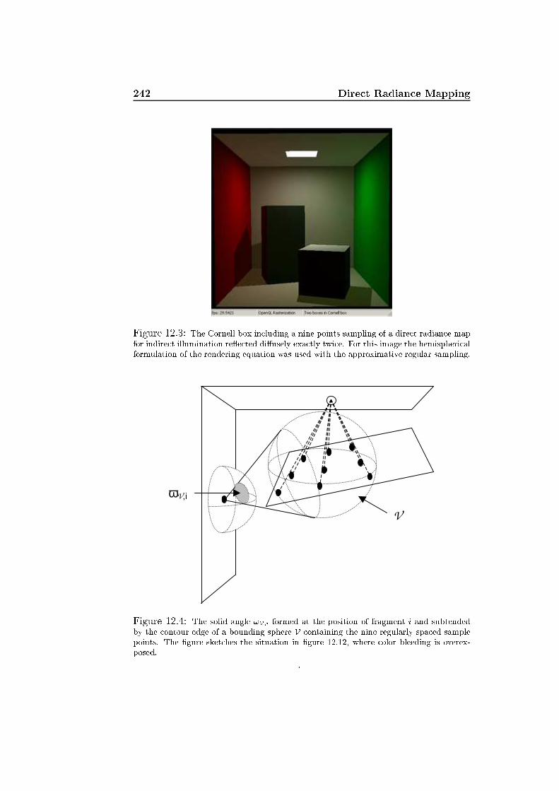
242 Dire t Radian e Mapping

Figure 12.3: The Cornell box in luding a nine points sampling of a dire t radian e mapfor indire t illumination re�e ted di�usely exa tly twi e. For this image the hemispheri alformulation of the rendering equation was used with the approximative regular sampling.

ωV,i

V

Figure 12.4: The solid angle !V;i formed at the position of fragment i and subtendedby the ontour edge of a bounding sphere V ontaining the nine regularly spa ed samplepoints. The �gure sket hes the situation in �gure 12.12, where olor bleeding is overex-posed. .

12.2 The Resulting Method 243

V

ωV,i

rV �cV − pi

�

α

pi

cV

Figure 12.5: If the bounding volume V is a bounding sphere, the solid angle !V;isubtended by the sphere an be found using spheri al oordinates.(see se . 5.1) we ould �nd this bounding volume V and either approximatethe solid angle (whi h may be di�erent for ea h fragment) by the solid angle!V; formed at the enter of the s ene and subtended by V, or we ould sendthe bounding volume down the pipeline and ompute !V;i for ea h fragment.In any ase a better PDF for (12.7) is given as:pi(!0) = 1!V;i � 1!V; Suppose we let V be a bounding sphere given by a enter V and aradius rV . Then the solid angle formed at the position pi of fragment i andsubtended by V ould be found in spheri al oordinates as shown in �gure12.5. Re alling (3.10) from the des ription of solid angles in se tion 3.2, we an �nd the solid angle as follows:! = Z 2�0 Z �0 sin � d� d� = 2�(1� os�)where � is the angle shown in �gure 12.5, whi h means that:!V;i = 2�(1 � qk V � pik2 � r2Vk V � pik )If we let V be an AABB, we ould approximate os� by the angularvisibility between the point pi and V (angular visibility was des ribed inse tion 11.1).

244 Dire t Radian e MappingAnother way to get an integral estimator of the re�e ted radian e isto use the area formulation of the rendering equation. If we let the PDFdenote uniform sampling a ross the surfa es in the dire t radian e map,p(x) = 1=AM , where AM is the area of the surfa es in the map, the resultingestimator will be:hLr(x;!)i = 1N NXi=0 �r;i� Lr;0;i(nx � !0i)(ny � �!0i)r2xyp(x)= AMN NXi=0 �r;i� Lr;0;i(nx � !0i)(ny � �!0i)r2xy (12.8)It should be noti ed that the normal is now needed in the dire t radian emap as well as it is in ea h fragment that we render. This means thatthe map must ontain a third texture holding the normal asso iated withthe interse ted surfa e lo ation. Also re all from se tion 5.1 that a polygon lose to the amera may �ll out the entire image and a polygon very far awaymay �ll out a single pixel only. This indi ates that al ulation of the areaof the surfa es seen in the dire t radian e map AM not ne essarily is doneeasily.If we approximate AM by a onstant and pla e an obje t lose to the lightsour e, the indire t light will again be heavily overexposed, sin e the a tualarea seen from the light sour e is not very large. Besides this problem (12.8)also results in a more expensive fragment program than the one needed toevaluate (12.7). In any ase �gure 12.6 shows an image found using (12.8)and a onstant approximation of AM for omparison with �gure 12.3.An idea for a rough approximation of AM is to take the value v0 of thetexel at position (0; 0) and the value v1 of the texel at position (1; 1) (the�rst and last) in the texture holding �rst interse tion points, and �nd thesquared distan e between the two points that they return:AM � (v1 � v0) � (v1 � v0)This ould be done at the appli ation stage (see se . 5.1) and supplied to thefragment program as a uniform parameter ea h frame.In both ases, the low number of samples makes the estimate quite frag-ile. The few sampling points learly show themselves when we use the areaformulation as seen in �gure 12.6. The remaining indire t illumination is,however, more orre t than in �gure 12.3. When using the hemispheri- al formulation of the rendering equation, the sampling problems will showthemselves in the overall indire t illumination (instead of at spe i� points).Putting an obje t exa tly where a sample is taken will result in a signi� ant hange in the indire t illumination. This an ause �i kering while obje tsare moving.

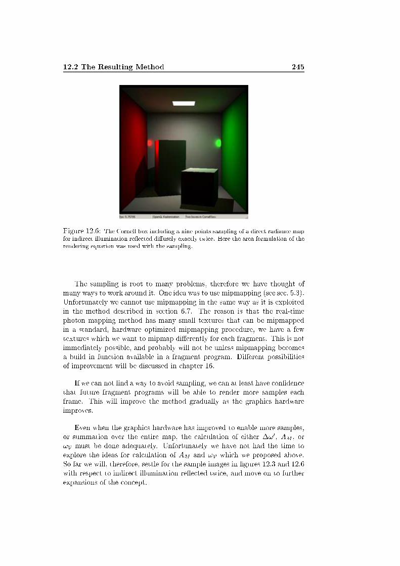
12.2 The Resulting Method 245

Figure 12.6: The Cornell box in luding a nine points sampling of a dire t radian e mapfor indire t illumination re�e ted di�usely exa tly twi e. Here the area formulation of therendering equation was used with the sampling.The sampling is root to many problems, therefore we have thought ofmany ways to work around it. One idea was to use mipmapping (see se . 5.3).Unfortunately we annot use mipmapping in the same way as it is exploitedin the method des ribed in se tion 6.7. The reason is that the real-timephoton mapping method has many small textures that an be mipmappedin a standard, hardware optimized mipmapping pro edure, we have a fewtextures whi h we want to mipmap di�erently for ea h fragment. This is notimmediately possible, and probably will not be unless mipmapping be omesa build in fun tion available in a fragment program. Di�erent possibilitiesof improvement will be dis ussed in hapter 16.If we an not �nd a way to avoid sampling, we an at least have on�den ethat future fragment programs will be able to render more samples ea hframe. This will improve the method gradually as the graphi s hardwareimproves.Even when the graphi s hardware has improved to enable more samples,or summation over the entire map, the al ulation of either �!0, AM , or!V must be done adequately. Unfortunately we have not had the time toexplore the ideas for al ulation of AM and !V whi h we proposed above.So far we will, therefore, settle for the sample images in �gures 12.3 and 12.6with respe t to indire t illumination re�e ted twi e, and move on to furtherexpansions of the on ept.

246 Dire t Radian e Mapping

Figure 12.7: The Cornell box rendered using dire t radian e mapping ombined withre ursive environment mapping. The two boxes have been repla ed by spheres having thefollowing materials. From left to right: (a) Two hrome (or mirror) spheres. (b) A hromeand a glass sphere.Arbitrary BRDFsSuppose we let the normals asso iated with the interse tion points be a partof the dire t radian e map, as is the ase if we use the area formulation ofthe rendering equation for sampling as des ribed above. Then storing thepure material olor instead of the re�e ted radian e in our dire t radian etexture, would make it possible (if enough pro essing power is available forea h sample in ea h fragment) to model an arbitrary BRDF. Even moretextures might be needed for the dire t radian e map, su h as one holdingthe dire tion of in iden e if more than one light sour e exist, and one holdingthree material parameters for BRDF al ulation at the �rst interse tion pointfrom the light sour e. This expansion is very expensive, at urrent hardwareit qui kly results in fragment programs ex eeding the allowed number ofinstru tions, nevertheless, it indi ates that arbitrary BRDFs an be modeledusing dire t radian e mapping.Perfe tly Spe ular Re�e tionsAs des ribed in se tion 6.3 spe ular re ursions an be handled in real-timeusing environment mapping. Combining this approa h with the dire t illu-mination, and the di�use illumination re�e ted twi e, we do, as previouslymentioned, end up with a method able to model the light paths: LS*DDS*Eand LD?S*E. Some results are shown in �gure 12.7, where the boxes arerepla ed by two spheres.

12.2 The Resulting Method 247

Figure 12.8: A glossy e�e t is obtained by adding indire t illumination to otherwiseperfe tly spe ular obje ts. From left to right: (a) The planar mirror in the ave s eneex luding the glossy e�e t. (b) The planar mirror in the ave s ene in luding the glossye�e t.An Inexpensive Glossy E�e tAn inexpensive way to make perfe tly spe ular surfa es (su h as the spheresin �gure 12.7) look glossy, is to simulate that the obje t is di�use withrespe t to indire t illumination. The dire t illumination is repla ed by the olor found in the re�e ted dire tion, but the di�usely re�e ted indire tillumination is added to the obje t. Sin e no perfe tly spe ular obje ts existin real life, this method gives mirrors a natural feeling, see �gure 12.8.Multiple Boun esAn expansion of the method following the multi-agent line of thought (seese . 11.4) would, as mentioned in se tion 12.1, be to let ea h obje t havean environment map of the radian e in its surroundings. The idea is thento add a few samples of indire t illumination from the environment map(sampled a ording to the BRDF) to the �nal shade of ea h fragment thatwe render. In luding fragments rendered when the environment maps areupdated. In this way the indire t illumination will in lude more boun esfor ea h frame rendered, in a way analogous to the re ursive environmentmapping for perfe tly spe ular surfa es. Unfortunately we had this ideatoo late to have time for an implementation. The method seems appealingex ept for the fa t that the frame rate will de rease as the number of obje tsin the s ene in reases, be ause ea h new obje t will need another six imagesfor update of an environment map ea h frame.Another idea is to sample in the previous image taken from the eye pointwhen drawing the texture of radian e from the light sour e, There are several

248 Dire t Radian e Mapping

Original objects

Center

Subsurface scaling

Center Problem

Object A Object B Figure 12.9: The s aling for real-time subsurfa e s attering. Sin e s aling is around the enter problems an easily o ur as illustrated through obje t B.limitations to this approa h though. First, only obje ts seen from the eyepoint or from a light sour e an have an in�uen e on the illumination in as ene. Se ond, only re�e tions o� perfe tly di�use surfa es would be possible.The reason is that if we use an arbitrary BRDF as des ribed above we needa texture with pure material olor instead of radian e, whi h is in ompatiblewith the on ept.Subsurfa e S atteringThe original idea for an expansion of DRM to in lude subsurfa e s attering(see se tion 12.1) was to expand the network by randomly jittered nodesstored inside a translu ent obje t. Sin e the network has no a tual existen e(only an abstra t existen e) in our implementation of the method we had toalter the on ept a bit.A ording to [60℄ the re ipro al of the extin tion oe� ient (des ribedin se tion 3.4) orresponds to the average distan e that a photon will movethrough a medium before intera tion:d = 1�tUsing this average distan e it is our idea to s ale a translu ent obje tuniformly around its enter to the size 1� d and draw it inside the originalobje t, see �gure 12.9. Unfortunately there is a problem in this simples aling, sin e the s aled obje t may end up outside the original obje t asseen in the �gure. To solve this approximately, the sten il bu�er is used tomark the original obje t and only the part of the s aled obje t whi h endsup inside the original obje t will be stored.To ontinue the on ept of dire t radian e mapping, the radian e in identon the diminished version of the original obje t, whi h represents subsurfa es attered light, is also found as an image from the light sour e and stored asa texture in the dire t radian e map.

12.2 The Resulting Method 249For simpli ity we only model the �rst interse tion below the surfa e ofthe obje t and we assume that this interse tion takes pla e at the averagedistan e. These approximations result in an opti al depth whi h equalsunity: �(s; s0) = Z ss0 �t(t)dt � �t�s � �td = 1If we do not take in-s attered light into a ount, but only dire t radian esubsurfa e s attered on e, the attenuated radian e rea hing the diminishedobje t will be given as follows:Lsubsurf = (1� Fr)e�1Li;1where Fr denotes the Fresnel re�e tan e.The point is, now, that we an render a subsurfa e s attered illuminationterm for all translu ent obje ts and add it to the dire t and indire t illumi-nation terms found previously. This is done by onsidering the radian etransported to the diminished obje t representing light s attered beneaththe surfa e on e. When looking at the surfa e of a translu ent obje t the in-tegral �nding in-s attered light at the surfa e lo ation an be approximatedby a sampling of the subsurfa e s attered light.The simplest way to �nd a ontribution from the subsurfa e s atteredlight is to use a single sample. We let the enter of a translu ent obje t beproje ted in the dire tion towards the light sour e into a position in the dire tradian e map. This position in the dire t radian e map will usually alsospe ify a position in the subsurfa e s attered illumination. Letting this singlesample ompute the ontribution from the subsurfa e s attered illuminationresults in the following: Li = e��t�s �s p(�)Lsubsurfwhere �t is the extin tion oe� ient, �s is the s attering oe� ient, andp(�) = 1=(4�) is the fa e fun tion (we have hosen to work with isotropi s attering only). �s is found as the distan e between the subsurfa e s at-tered position and the surfa e position.This extremely simple version of subsurfa e s attering has some reason-able results. Of ourse the illumination is mostly in orre t, but the visual ue ertainly exists, see �gure 12.10 for a omparison between a s ene wherethe subsurfa e s attering is in luded and a s ene where it is not.It should be noted that the subsurfa e s attering requires two extra tex-tures in the dire t radian e map: One for subsurfa e radian e and one forsubsurfa e positions.At the expense of pro essing time, the sampling ould be in reased tohave a better estimate of the subsurfa e s attered illumination.

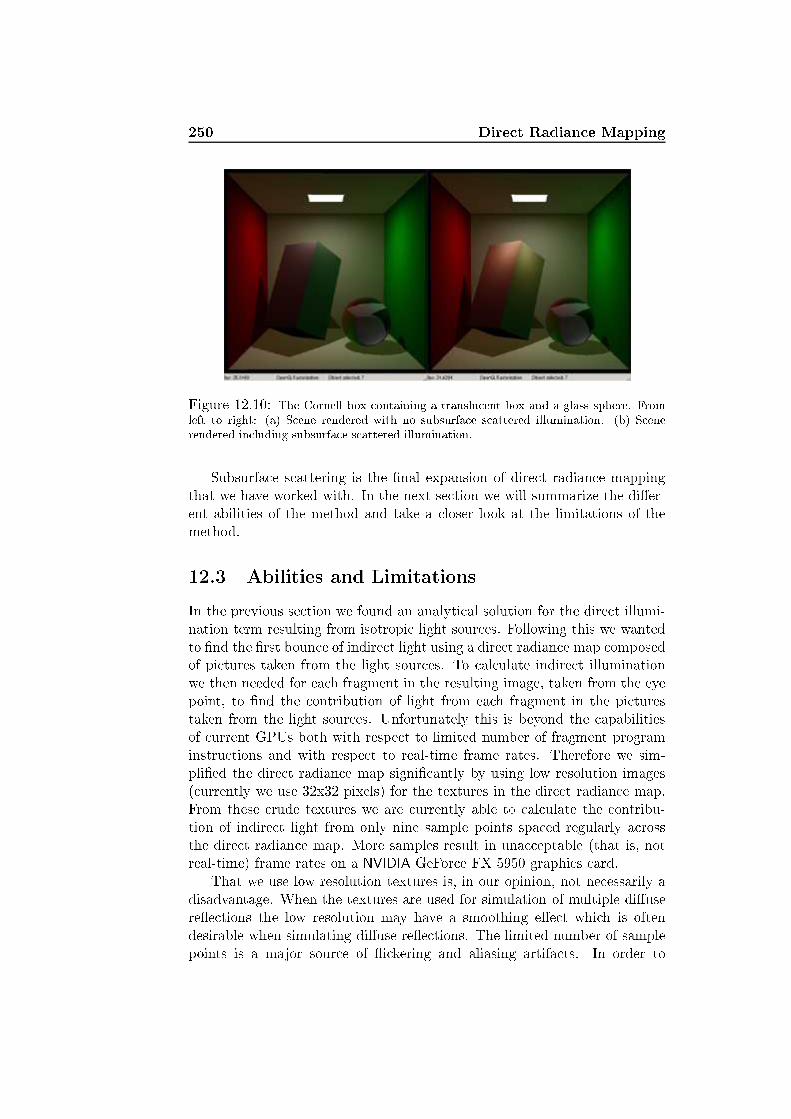
250 Dire t Radian e Mapping

Figure 12.10: The Cornell box ontaining a translu ent box and a glass sphere. Fromleft to right: (a) S ene rendered with no subsurfa e s attered illumination. (b) S enerendered in luding subsurfa e s attered illumination.Subsurfa e s attering is the �nal expansion of dire t radian e mappingthat we have worked with. In the next se tion we will summarize the di�er-ent abilities of the method and take a loser look at the limitations of themethod.12.3 Abilities and LimitationsIn the previous se tion we found an analyti al solution for the dire t illumi-nation term resulting from isotropi light sour es. Following this we wantedto �nd the �rst boun e of indire t light using a dire t radian e map omposedof pi tures taken from the light sour es. To al ulate indire t illuminationwe then needed for ea h fragment in the resulting image, taken from the eyepoint, to �nd the ontribution of light from ea h fragment in the pi turestaken from the light sour es. Unfortunately this is beyond the apabilitiesof urrent GPUs both with respe t to limited number of fragment programinstru tions and with respe t to real-time frame rates. Therefore we sim-pli�ed the dire t radian e map signi� antly by using low resolution images( urrently we use 32x32 pixels) for the textures in the dire t radian e map.From these rude textures we are urrently able to al ulate the ontribu-tion of indire t light from only nine sample points spa ed regularly a rossthe dire t radian e map. More samples result in una eptable (that is, notreal-time) frame rates on a NVIDIA GeFor e FX 5950 graphi s ard.That we use low resolution textures is, in our opinion, not ne essarily adisadvantage. When the textures are used for simulation of multiple di�usere�e tions the low resolution may have a smoothing e�e t whi h is oftendesirable when simulating di�use re�e tions. The limited number of samplepoints is a major sour e of �i kering and aliasing artifa ts. In order to

12.3 Abilities and Limitations 251in rease the number of sample points we ould distribute the al ulationover multiple frames, so that only part of the light was al ulated in ea hframe. This would give a low sampling rate approximation when things movedynami ally and a ontinuously improving image while amera and obje tsstay stati . The �i kering will still be apparent sin e it is mostly visible whenthings move around dynami ally.Our limited implementation of the method approximates !V and AM by onstants. This results in a heavy overexposure of indire t illumination whenobje ts move lose to the light sour e. We proposed approximate solutionsfor this problem in the previous se tion, but have not had the time to testthese solutions. Therefore the overexposure will show itself when using thedemonstration appli ation (see �gure 12.12). We see this not as a limitationto the method, but rather as a te hni ality whi h we an �nd a solution for.In the following we will �rst list the abilities and afterwards problemsand limitations of dire t radian e mapping. Both have been indi ated in theprevious se tions, therefore we will only sum them up shortly. The abilitiesare:� Dire t radian e mapping is a method for reating indire t illuminationin real-time. In real-time we are able to al ulate an approximationof the �rst boun e of di�usely re�e ted indire t illumination in ea hframe. This enables visual e�e ts su h as olor bleeding.� The method is independent of number of verti es in the s ene, meaningthat it is bounded by the number of fragments rather than the numberof verti es when rendering.� Sin e we re al ulate all illumination terms for ea h frame, obje ts andlight sour es an move about freely in the s ene.� The method is independent of the geometry in the s ene, that is, wedo not have to onsider the shape or omplexity of an obje t.� Our method is based on the GPU, meaning that CPU pro essing poweris left for other purposes and that the method will improve as graphi s ards improve.� Many extensions have been proposed giving ri h opportunity for betterversions of the rendering method.Although the above apa ities sound appealing there is also a ba k side ofthe medal. We will now dis uss the problems and limitations to our urrentimplementation method. Along the way we will suggest possible solutionsto the problems or des ribe what it would take to solve them. The problemsand limitations are:

252 Dire t Radian e Mapping� Only �rst boun e is al ulated� We assume that all obje ts are di�use while al ulating the indire tillumination.� Indire t light is al ulated in a lo al illumination manner, in otherwords we do not take indire t shadows into a ount.� The method is fragment bound.� (The dire t radian e map is low resolution.)� Only a low sampling rate is a�ordable in the al ulation of indire tillumination using the dire t radian e map. And the same samplepoints are used in all fragments.� !V or AM is approximated by a onstant.The limitations result in a number of artifa ts in the s ene. Some appearalways others are not visible until the s ene be omes dynami . We will nowgo through these one by one and dis uss them.As long as only the �rst boun e is al ulated some indire t illuminationwill, of ourse, be missing. The result is an image, whi h is a little darkerthan would have been the ase if we had in luded multiple light boun es.Proposals for multiple boun es were given in the previous se tion.The assumption that all obje ts are di�use is not a fundamental ne essityfor the method. It is merely assumed in the implementation for e� ien yreasons. Expansion to arbitrary BRDFs is also des ribed in the previousse tion.The fa t that we do not onsider visibility in the estimate of the di�uselyre�e ted illumination term results in a number of artifa ts. One problemis visualized in �gure 12.11 showing a s reen shot of the ave s ene. Herethe room behind the door is illuminated by indire t lighting, whi h is not orre t, sin e the door should keep the room ompletely o luded. The erroro urs be ause indire t light is al ulated in a lo al illumination mannerwhere obje ts blo king the path of the indire t illumination are not takeninto onsideration. To avoid this problem we must take indire t shadowsinto onsideration in the al ulations. A solution is not straightforward. Theproposal of an environment map for ea h obje t, whi h an model multiplelight boun es, will also in lude indire t shadows. This approa h is maybethe best solution.The method does not so mu h depend on the number of triangles orverti es in the s ene, whi h allow us to reate ompli ated s enes withoutloosing too mu h frame rate. In ontrast the method is bound by the numberof pixels that needs to be rendered, or in other words the method is frag-ment bound. This means that the higher s reen resolution we use the lower

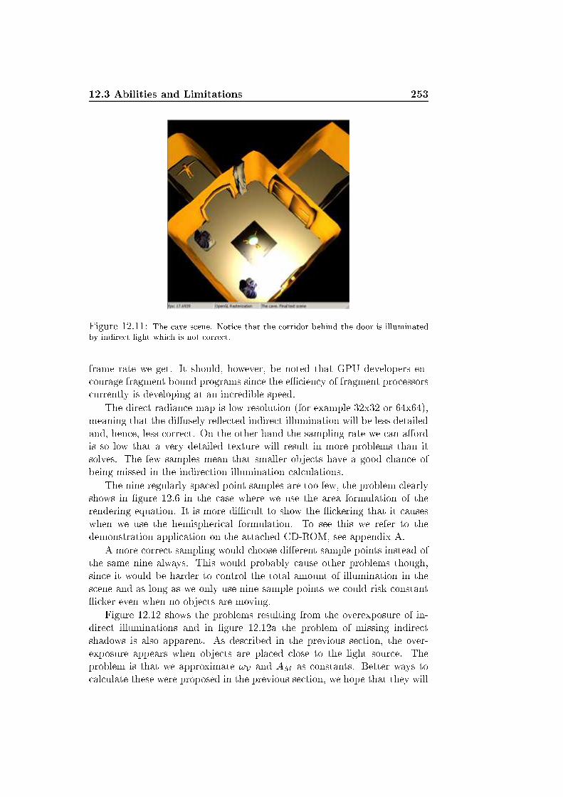
12.3 Abilities and Limitations 253

Figure 12.11: The ave s ene. Noti e that the orridor behind the door is illuminatedby indire t light whi h is not orre t.frame rate we get. It should, however, be noted that GPU developers en- ourage fragment bound programs sin e the e� ien y of fragment pro essors urrently is developing at an in redible speed.The dire t radian e map is low resolution (for example 32x32 or 64x64),meaning that the di�usely re�e ted indire t illumination will be less detailedand, hen e, less orre t. On the other hand the sampling rate we an a�ordis so low that a very detailed texture will result in more problems than itsolves. The few samples mean that smaller obje ts have a good han e ofbeing missed in the indire tion illumination al ulations.The nine regularly spa ed point samples are too few, the problem learlyshows in �gure 12.6 in the ase where we use the area formulation of therendering equation. It is more di� ult to show the �i kering that it auseswhen we use the hemispheri al formulation. To see this we refer to thedemonstration appli ation on the atta hed CD-ROM, see appendix A.A more orre t sampling would hoose di�erent sample points instead ofthe same nine always. This would probably ause other problems though,sin e it would be harder to ontrol the total amount of illumination in thes ene and as long as we only use nine sample points we ould risk onstant�i ker even when no obje ts are moving.Figure 12.12 shows the problems resulting from the overexposure of in-dire t illuminations and in �gure 12.12a the problem of missing indire tshadows is also apparent. As des ribed in the previous se tion, the over-exposure appears when obje ts are pla ed lose to the light sour e. Theproblem is that we approximate !V and AM as onstants. Better ways to al ulate these were proposed in the previous se tion, we hope that they will

254 Dire t Radian e Mapping

Figure 12.12: The problems resulting from approximation of !V and AM by a onstant.When obje ts are pla ed lose to the light sour e, indire t illumination gets overexposed.From left to right: (a) The green wall of the Cornell box moved lose to the light sour e.The indire t illumination is approximated by the hemispheri al formulation of the render-ing equation. Here the missing indire t shadows are also apparent. (b) The same as (a)only using the area formulation of the rendering equation.solve the problem in a reasonable way.As the �nal part of this se tion we will brie�y dis uss our simpli�edapproa h to subsurfa e s attering.Using the on epts of dire t radian e mapping we have reated a veryminimal simulation of subsurfa e s attering. The out ome of this method isnot quite pre ise enough for a detailed omparison with other methods (su has those des ribed in se tion 3.4) reating subsurfa e s attering in real-time(or at intera tive rates).Very few experiments have been arried out with the method as we havemainly on entrated our e�orts on indire t illumination. This leaves us withseveral orre tions and improvements whi h ould be ontributed to the sub-surfa e s attering implementation. A few will brie�y be mentioned in thefollowing while we des ribe some of the problems and limitations to themethod for subsurfa e s attering whi h we presented in the previous se tion.First of all we an only a�ord to use one sample point to al ulate thesubsurfa e s attering of an obje t. This is the main reasons why the subsur-fa e s attered light often looks somewhat odd. More sample points wouldbe bene� ial but as it is now they are too expensive with regards to theframe rate, at least if we want to ombine the subsurfa e s attering with theindire t illumination.Another problem is the simpli�ed way in whi h we reate the inner obje t.Sin e we s ale the obje t towards its enter we risk that parts of it is ut awaybe ause it falls outside of the original obje t ( f. �g. 12.9). This means thatfrom unfortunate angles the subsurfa e s attering e�e t disappears entirely,if the sample point is set where there is no inner obje t available. A better

12.4 Comparison 255way to s ale the obje t would be to translate ea h vertex in a negativedire tion from its normal. In this way the inner obje t would never omeoutside the boundaries of the original obje t (unless it is translated all theway through the obje t and out through the surfa e on the opposite side).Sin e the inner obje t is an exa t repli ate of the original obje t (onlysmaller) the distan e to the surfa e will always be the same. It might give amore realisti e�e t if the distan e ould vary a little. An idea for generatinga more s attered distan e is to put several s aled obje ts inside ea h otherand then pi k a random one. In this way we ould have an arbitrary numberof layers with di�erent distan es to the surfa e to pi k from randomly. To reate e�e ts even loser to the original physi s we ould establish boun esbetween the layers as well. However this would probably be an expensivepro edure.After a dis ussion of the most important drawba ks let us return towhat we have a omplished. We are able to �nd the �rst boun e of indire tlight in an arbitrary s ene no matter how omplex the obje ts are. Thelight is re al ulated at a frame rate of 10-30 fps (see the lower left ornerof the di�erent s reen shots, or try out the appli ation). Moreover we haveproposed a simple version of subsurfa e s attering, whi h gives reasonableresults and many options for improvements taking the many simplifyingassumptions into a ount. The next se tion will ompare the method toother implementations that we have ome a ross in the literature study ofthis proje t.12.4 ComparisonDire t radian e mapping is mainly a method for real-time simulation of thepart of the rendering equation, whi h in se tion 4.4 is des ribed as the multi-ple di�use re�e tions term. Other methods are able to do the same; some ofthese are des ribed in hapter 6. This se tion will ompare dire t radian emapping to ea h of the methods des ribed in se tions 6.6, 6.7, 6.8, and 6.9with respe t to the ability to simulate the multiple di�use re�e tions term.The methods will be ompared to dire t radian e mapping one by one.Light Maps vs. Dire t Radian e MappingThe light map method uses pre- al ulated global illumination (most oftenradiosity) to apply indire t illumination in a s ene. The illumination is stati but in di�use environments it provides a good visual e�e t even if it does not hange a ording to the surroundings. The method is used in several newergames; an example is given in [109℄. A basi assumption of light maps is that,as long as the light sour es are stati and not parti ularly remarkable, thefa t that di�usely re�e ted indire t illumination is stati is not noti eable.This is often true in a game s enario where swift movement is frequently

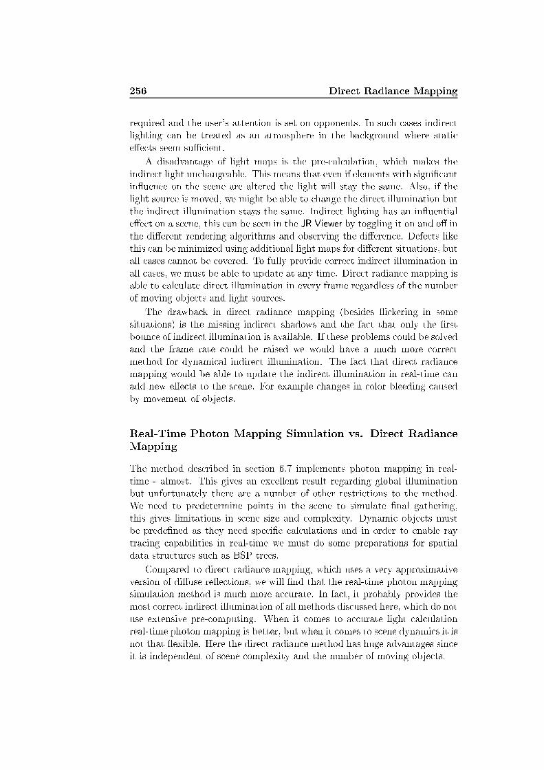
256 Dire t Radian e Mappingrequired and the user's attention is set on opponents. In su h ases indire tlighting an be treated as an atmosphere in the ba kground where stati e�e ts seem su� ient.A disadvantage of light maps is the pre- al ulation, whi h makes theindire t light un hangeable. This means that even if elements with signi� antin�uen e on the s ene are altered the light will stay the same. Also, if thelight sour e is moved, we might be able to hange the dire t illumination butthe indire t illumination stays the same. Indire t lighting has an in�uentiale�e t on a s ene, this an be seen in the JR Viewer by toggling it on and o� inthe di�erent rendering algorithms and observing the di�eren e. Defe ts likethis an be minimized using additional light maps for di�erent situations, butall ases annot be overed. To fully provide orre t indire t illumination inall ases, we must be able to update at any time. Dire t radian e mapping isable to al ulate dire t illumination in every frame regardless of the numberof moving obje ts and light sour es.The drawba k in dire t radian e mapping (besides �i kering in somesituations) is the missing indire t shadows and the fa t that only the �rstboun e of indire t illumination is available. If these problems ould be solvedand the frame rate ould be raised we would have a mu h more orre tmethod for dynami al indire t illumination. The fa t that dire t radian emapping would be able to update the indire t illumination in real-time anadd new e�e ts to the s ene. For example hanges in olor bleeding ausedby movement of obje ts.Real-Time Photon Mapping Simulation vs. Dire t Radian eMappingThe method des ribed in se tion 6.7 implements photon mapping in real-time - almost. This gives an ex ellent result regarding global illuminationbut unfortunately there are a number of other restri tions to the method.We need to predetermine points in the s ene to simulate �nal gathering,this gives limitations in s ene size and omplexity. Dynami obje ts mustbe prede�ned as they need spe i� al ulations and in order to enable raytra ing apabilities in real-time we must do some preparations for spatialdata stru tures su h as BSP trees.Compared to dire t radian e mapping, whi h uses a very approximativeversion of di�use re�e tions, we will �nd that the real-time photon mappingsimulation method is mu h more a urate. In fa t, it probably provides themost orre t indire t illumination of all methods dis ussed here, whi h do notuse extensive pre- omputing. When it omes to a urate light al ulationreal-time photon mapping is better, but when it omes to s ene dynami s it isnot that �exible. Here the dire t radian e method has huge advantages sin eit is independent of s ene omplexity and the number of moving obje ts.

12.4 Comparison 257Pre- omputed Radian e Transfer vs. Dire t Radian e Map-pingIn pre- omputed radian e transfer a large part of the al ulations are arriedout in advan e. The result of the pre- omputation is a method apable ofsimulating almost any type of visual e�e t on a single obje t, even in a framerate useful for ommer ial appli ations su h as omputer games. However,the method still has some limitations; it must assume that obje ts are rigid,otherwise pre- omputation of global illumination would not be possible, andas des ribed in se tion 6.8 the method has problems the moment severaldynami obje ts need to intera t in the same s ene. These are both issuesthat do not a�e t dire t radian e mapping sin e it is independent of thes ene geometry.In other words the most important drawba ks of pre- omputed radian etransfer are the limitations regarding intera tion between dynami obje tsand the massive pre- omputations needed. The advantage of pre- omputedradian e transfer is the quality of the global illumination, whi h is only vi -tim of the limitations in spheri al harmoni s basis fun tions. Pre- omputedradian e transfer is good for simple s enes raving detailed illumination, su has a talking person. In omparison dire t radian e mapping has almost oppo-site features. While there is no restri tions on s ene dynami s, the di�uselyre�e ted indire t illumination is rude and impre ise.Environment Map Rendering vs. Dire t Radian e MappingThe method, whi h we have hosen to all environment map rendering2builds on the same philosophy with respe t to s ene dynami s as does dire tradian e mapping. Therefore it has many of the same advantages as dire tradian e mapping.Environment map rendering (in the sense of Nijasure et al. [93℄) is doneby estimation of radian e transfer fun tions at the nodes of a regular gridspa ed throughout the s ene. The transfer fun tions are represented in aspheri al harmoni s basis and estimated using environment maps. For ea hlo ation in the s ene to be rendered an interpolation between the nearesttransfer fun tions should de ide the illumination at that spe i� lo ation.The problemati issues are the regular grid, the interpolation, and theusual limitations to spheri al harmoni s representation of transfer fun tions.First, the resolution of the regular grid depends on s ene omplexity. We an ompare the nodes of the grid where environment maps are found tothe sample points in dire t radian e mapping. The interpolation an ausesome olor or shadow leakage through walls for example, whi h is again also onne ted to the spheri al harmoni s representation of the transfer fun tions.2No parti ular name has been given to the method by its authors.

258 Dire t Radian e MappingThe inventors of the method suggest solutions for most of these problems(for more details see se . 6.9).All in all environment map rendering is a method having apabilitiessimilar to dire t radian e mapping. It also has some problems, but seeminglythey are few. The frame rates are a bit lower (approximately 10 fps), but theresult is more orre t. The solution suggested for olor and shadow leakage an not yet run in hardware. Nevertheless, the environment map renderingmethod presented by Nijasure et al. is a tough ompetitor to dire t radian emapping. Nijasure's method probably gets the upper hand.SummaryThe omparisons are summarized in table 12.1, whi h presents positive fea-tures of the di�erent methods as we see them. The features listed should beseen with regards to the multiple di�use re�e tions term only. For exam-ple it is possible to have dynami obje ts in s enes using the light mappingmethod but the indire t light does not hange with them.Some markings are set in parentheses, this illustrate that there are ertain onditions that must be ful�lled before it is true. The following list shortlysum up these restri tions.� Real-time photon mapping simulation supports an arbitrary numberof dynami obje ts, but the dynami obje ts must be pointed out inadvan e.� In the des ription of real-time photon mapping it is stated that di�useobje ts must be assumed. This is, however, only ne essary in the lastboun e of the indire t illumination, sin e interpolation between pointsdistributed in the s ene is used. At all light boun es ex ept the se ondto last di�use intera tion an arbitrary BRDF an be employed.� Pre- omputation does o ur in the real-time photon map simulationmethod, but only of BSP trees for speeding up the rendering pro ess.� Pre- omputed radian e transfer supports both perfe tly di�use andglossy BRDFs. An inherent limitation to the spheri al harmoni s ap-proa h used in pre- omputed radian e transfer, is that the loser theBRDF omes to a perfe tly spe ular BRDF, the more spheri al har-moni s basis fun tions will the method need to model the re�e tionwithout serious aliasing artifa ts. Therefore pre- omputed radian etransfer only supports low-frequen y lighting environments.� Indire t shadows are supported in the environment map renderingmethod, but only if the method is implemented in software (not inhardware).

12.4 Comparison 259� Environment map rendering uses spheri al harmoni s in the same wayas pre- omputed radian e transfer, hen e, it is subje t to the samerestri tions regarding BRDFs.Looking at the table we �nd that methods building on pre- omputationare the ones urrently fast enough to be used in ommer ial appli ations.However, there are ertain restri tions to them that are only fully solvedusing methods that do not need pre- al ulations. On this observation wedare predi t that other methods based on GPU intensive rendering will winin time (at least in some situations).Another thing revealed from the table is ertain drawba ks of the dire tradian e mapping in features supported by other methods. In the report wehave suggested solutions to many of these drawba ks, others might be solvedby ombination of our method with some of the others. Parti ularly inter-esting ould be a ombination of dire t radian e mapping and environmentmap rendering as the two methods builds on the same philosophy arriedout a bit di�erently. Although the table reveals fewer apabilities in someareas for dire t radian e mapping ompared to the other methods we stillhave faith in the idea, as it is at an early state of development.This on ludes our presentation of dire t radian e mapping. The next hapter will shortly des ribe the di�erent traditional rendering methods thatwe have implemented for referen e.

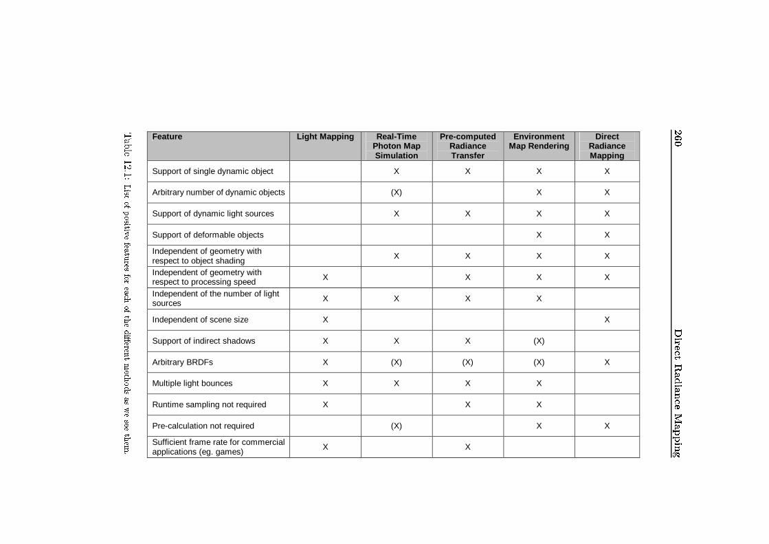
260Dire tRadian eMapping

Feature Light Mapping Real-Time Photon Map Simulation

Pre-computed Radiance Transfer

Environment Map Rendering

Direct Radiance Mapping

Support of single dynamic object X X X X

Arbitrary number of dynamic objects (X) X X

Support of dynamic light sources X X X X

Support of deformable objects X X

Independent of geometry with respect to object shading

X X X X

Independent of geometry with respect to processing speed X X X X

Independent of the number of light sources X X X X

Independent of scene size X X

Support of indirect shadows X X X (X)

Arbitrary BRDFs X (X) (X) (X) X

Multiple light bounces X X X X

Runtime sampling not required X X X

Pre-calculation not required (X) X X

Sufficient frame rate for commercial applications (eg. games)

X X

Table12.1:Listofpositivefeaturesforea hofthedi�erentmethodsasweseethem.

Chapter 13Other Implemented RenderingMethods

Virtue is never isolated; it always has neighbors.Confu ius (552-479 BC.): Anale ts 4:25

262 Other Implemented Rendering MethodsSin e it was the original idea for this proje t to ombine photorealisti ren-dering and real-time rendering by having an implementation in ea h amp,we started out onstru ting a ray tra er and added di�erent optimizationss hemes of our own (des ribed in hap. 11) before implementing our real-timerenderer.The result of this pro edure is that we have implemented a fairly fun -tional ray tra er as well as other global illumination methods, whi h we anuse as referen e for our results from dire t radian e mapping (DRM). Thedrawba k is perhaps that by putting fo us in two pla es we have not beenable to go as deep into one subje t as we ould have. On the other handwe feel that working with traditional photorealisti rendering has given us abetter fundament for the real-time implementation; in fa t, we think that itis doubtful whether we would have ome up with any of the ideas presentedin hapters 11 and 12, if we had not followed this pro edure.In this hapter we will des ribe rendering features implemented besideDRM. Se tion 13.1 will mention the rendering methods that have been im-plemented for photorealisti rendering, and se tion 13.2 will point out themethods that have been implemented for ombination with DRM in ourreal-time renderer.13.1 Photorealisti Rendering MethodsRadiosity, ray tra ing, and photon mapping have all been implemented andare available in the appli ation a ompanying this report. Ea h of thesemethods have been implemented in a very simple version, sin e they aremainly there for referen e. In the following we will point out whi h parts ofea h method that have been implemented.RadiosityRadiosity is a simple implementation, whi h only in lude two approa hes:Radiosity using the simple analyti al approa h to the form fa tor al ulationgiven in (4.4), in this ase we do not onsider visibility between pat hes,and radiosity using the hemi ube method, where �ve pi tures are taken fordetermination of ea h form fa tor.A progressive re�nement approa h similar to the one des ribed in se -tion 4.1 is used to solve the system of linear equations. Our radiosity im-plementation features no expansions and is merely there for referen e whenwe simulate the multiple di�use re�e tions term using other methods. Sometypi al s reen shots of our radiosity implementation are shown in �gure 13.1.

13.1 Photorealisti Rendering Methods 263

Figure 13.1: S reen shot of the s ene pat hes for radiosity and the result of the hemi uberadiosity solution (as implemented for this proje t) applied to the Cornell box.Ray Tra ingA naïve one-ray-per-pixel ray tra er has been implemented. It follows thesame on epts as des ribed in se tion 4.2. The idea of angular visibility,des ribed in se tion 11.1, is always used with the ray tra er, sin e it improveson rendering times without ompromising image quality. Other spatial datastru tures have not been implemented. Hardware optimization as des ribedin se tion 11.7 has been implemented as well. It an be toggled on and o�,sin e it redu es image quality a little.Soft shadows have been implemented using Monte Carlo ray tra ing asdes ribed in se tion 4.3. A number of shadow rays (we use 50) are tra edtowards positions on a square area light sour e sampled using Quasi-MonteCarlo Halton sequen es (see eg. [141℄). The fra tion of these rays rea hingthe light sour e denotes the visibility term.The three simplest BRDFs have been implemented for shading in theray tra er. The BRDFs are alled Phong, Blinn-Phong, and Modi�ed Blinn-Phong. All of them are des ribed in se tion 5.2.Photon MappingPhoton mapping has been implemented as des ribed in se tion 4.4, ex eptwe have not found time for an implementation of �nal gathering. Insteadwe divide the photon map into four di�erent maps, one for ea h term thatwe wish to simulate. The four photon maps are used for dire t illumination, austi s, indire t illumination, and shadows respe tively.The austi s photon map is used as des ribed in 4.4. The indire t illu-mination map is used for a dire t visualization of the indire t illumination.This is not optimal sin e a dire t visualization of a photon map always re-sults in low frequen y noise. Our implementation is like this be ause we

264 Other Implemented Rendering Methodshad in mind to �lter the dire t visualization of the indire t illumination us-ing a neural network, our proje t moved in another dire tion though. Theshadow photon map is used for optimization of the soft shadow Monte Carloray tra ing operation. If no shadow photons are found nearby, we need not al ulate the visibility term we an merely set it to one.If �nal gathering was to be implemented we would need to have a globalphoton map, whi h would be a ombination of the dire t, austi s, andindire t maps.Some s reen shots of our ray tra ing solution in luding some photonmapping are given in �gure 13.2.These were, in short, the global illumination methods implemented andavailable through the JR Viewer (see hap. 14). In the next se tion we pointout the di�erent real-time rendering methods that we have implemented for ombination with dire t radian e mapping.

Figure 13.2: S reen shots of our ray tra ing solution applied to the Cornell box. Fromleft to right: (a) Ray tra ing in luding soft shadows and a austi s photon map. (b)The same as (a), but also in luding a dire t visualization of the photon map simulatingmultiple di�use re�e tions. Ex ept for the noise the se ondary austi s should be noti edbelow the glass sphere.13.2 Other Real-Time Rendering MethodsAs des ribed in hapter 6 many di�erent real-time methods an be ombinedin order to simulate di�erent rendering equation terms. The only rule to omply with is that no lass of light paths an be in luded more than on e.In this se tion we shortly point out the di�erent methods that we havemade available in our implementation for ombination with dire t radian emapping. We will also mention a few of the methods that advantageously ould have been ombined with dire t radian e mapping if we had had extratime for the implementation.

13.2 Other Real-Time Rendering Methods 265The basi real-time renderer implements the simple rasterization ap-proa h des ribed in hapter 5. The standard shading is Phong highlighting.The expansions are as follows: First urved and planar re�e tions have beenimplemented as des ribed in se tions 6.2 and 6.3. It is an option in the imple-mentation to use re ursive urved re�e tions. Se ond fragment shading hasbeen implemented for dire t illumination as an alternative to the standardPhong highlighting. Shadow volumes have been implemented as des ribedin se tion 6.1. Finally refra tions have been implemented for the spe ial aseof a sphere.Real-Time Glass Ball RenderingRefra tions are found using an environment map in the same way as for urved re�e tions only the refra ted dire tion should be used for texture oordinates rather than the re�e ted dire tion. In the spe ial ase of asphere the light refra ts twi e; on e at the �rst interse tion point and on ewhen the refra ted ray has passed through the sphere and is again refra tedba k into the environment.The �rst refra ted dire tion !t;1 is found using the refra tion formula(3.5). The refra tion formula is available as a hardware instru tion on mostGPUs. Now, to �nd the se ond refra ted dire tion !t;2 we must �nd thenormal, n2, at the se ond point of interse tion. Considering �gure 13.3 wequi kly realize that n2 is the normal, n1, at the �rst point of interse tionre�e ted in the dire tion opposite to the �rst refra ted dire tion �!t;1.

•

ωωωω

n2

n1

ωωωω t,2

ωωωω t,1

n1

Figure 13.3: Double refra tion through a sphere.

266 Other Implemented Rendering MethodsUsing the re�e tion formula (3.2) we get:n2 = 2(n1 � �!t;1)(�!t;1)� n1and sin e the environment map assumes that all dire tions used for tex-ture oordinates originate at the enter of the obje t, the se ond refra teddire tion an be found by the refra tion formula used between �!t;1 and n2.The refra tion should afterwards be blended with the re�e tion a ordingto the Fresnel re�e tan e. If we use the simpli�ed formula given in (3.36)and insert �1 = 1 for air outside the sphere and �2 = 1:5 orresponding tothe refra tion index of glass, we get the following simple Fresnel formula:Fr;glass(�) = 0:04 + 0:96(1 � os �)5where � is the angle of in iden e.Sphere Causti sCreating austi s in real-time for arbitrary obje ts is a di� ult task. Themost promising method we have found is the one presented in [74℄, whi his also des ribed shortly in se tion 6.4. Causti s for a simple primitive likea sphere, resulting from light emitted from a point light sour e, an beapproximated in a straightforward manner. To reate austi s in real-timefor a sphere we ould reate a one with an axis through the enter of thesphere. In a plane also through the enter of the sphere and perpendi ularto a line between the sphere enter and the light sour e, we ould mirror thelight one. The austi aused by the light will then appear where the oneinterse ts with another surfa e. The on ept is illustrated in �gure 13.4.

Sphere

Light source

Caustic Figure 13.4: A fast approximation of a sphere austi .The austi s area an be marked in the sten il bu�er and illuminationattenuated a ording to Fresnel re�e tan e an be added to the austi s area.

13.2 Other Real-Time Rendering Methods 267Similar simple assumptions about light traveling through other primitiveobje ts ould be reated. However, the method will not work for arbitraryobje ts and it gives only a rude approximation. To make real austi al- ulations, rays must be tra ed inside the obje t. In [74℄ it is des ribed howthis an be done in real-time. Unfortunately there has been no time inthis proje t for an implementation of real-time austi s (not even the rudesphere austi presented here).The remaining real-time rendering methods that have been implementedwere des ribed in hapter 12. In the following hapter we will give a presen-tation of the GUI that has been developed for the appli ation implementingthe di�erent rendering methods.

268 Other Implemented Rendering Methods

Chapter 14Graphi al User Interfa e

Un roquis vaut mieux qu'un long dis ours.Napoleon Bonaparte (1769-1821)

270 Graphi al User Interfa eMany proje ts on erning global illumination in real-time limit themselves toa proof of on ept only using prede�ned test s enes. This is, of ourse, quitealright, but if the method developed is to be appli able for a ommer ialappli ation, it must be able to ope with more omplex s enarios. To takethe proje t a little step further we have enabled a way to reate s enes ina modeling appli ation and then export them to a graphi al user interfa e(GUI) where our illumination methods an be tested on the s ene. This isa part of the se ond obje tive for this proje t in whi h we want to show thework �ow from modeling to real-time rendering using our own methodsSe tion 14.1 will des ribe the test s enes reated for the proje t. Ea hobje t in ea h s ene will be identi�ed and their purpose will be explained.About half of the test s enes are written dire tly in ode sin e they to a er-tain extent are ben hmark s enes (Cornell boxes ontaining di�erent simpleobje ts, the Cornell box data an be found in [95℄). The rest of the s enesare reated in Blender. How to use Blender is explained in hapter 10.The s enes are available through the windows GUI. How to use the GUIand all its features is overed in se tion 14.2.14.1 Test S enesTo demonstrate our implementations of rendering methods and to omparethem to ea h other we have reated a number of test s enes available througha small demonstration appli ation: The JR Viewer. In this se tion we presentthe test s enes one by one in order to explain what ea h of them is usefulfor.The s enes are available through the �le dropdown menu (see next se -tion). The following s enes an be sele ted:� Cornell Box - Empty� Cornell Box - Two Boxes� Cornell Box - Two Spheres� Cornell Box - Sphere and Box� (Cornell Box - Orb)� (Cornell Box - Arthur)� Cave S eneWe will now present the s enes one by one.

14.1 Test S enes 271Cornell Box - EmptyThe Cornell box is a omputer graphi s ben hmark s ene invented at theCornell University and used very frequently. The box is physi ally built anddetailed material parameters are measured from it. The data an be foundin [95℄. It is an almost quadrati box with one side open towards the amera.In this way an almost quadrati room is reated. The �oor, ba k wall and eiling are white (not purely white, just white), while the left wall is red andthe right wall is green (�gure 4.1 in hapter 4 shows a Cornell box with twoboxes inside it). The empty Cornell box is the simplest test s ene we haveand all rendering methods work for this s ene.Cornell Box - Two BoxesTraditionally the next level of omplexity for Cornell boxes is to pla e twoboxes in them, as a representation of simple obje ts. With the two boxeswe an better illustrate olor bleeding and shadows. Subsurfa e s attering isenabled for the tall box in the s ene for demonstration of our rude real-timeimplementation of this e�e t. The Cornell box with two boxes is the onlys ene besides the empty Cornell box that is available for radiosity rendering.This is be ause we transferred the radiosity implementation, as previouslymentioned, from a DTU ourse (02561) merely to have radiosity for referen e.The two boxes s ene is therefore well suited for olor bleeding omparison.Cornell Box - Two SpheresIn this s ene the two boxes are repla ed with two other simple obje ts:Spheres. The spheres have di�erent material parameters. The left sphereis a hrome (or mirror) sphere while the right sphere is a glass sphere. Thiss ene is made to demonstrate re�e tive and refra tive rendering methods reated for the proje t. When working in the rasterization menu (see next hapter) both spheres will have hrome material if refra tions are not en-abled.Cornell Box - Sphere and BoxThe Cornell box ontaining a sphere and a box ombines the box with sub-surfa e s attering and the refra tive sphere. This gives an opportunity totest (almost) all the di�erent rendering methods in the same s ene. In thisway we an also hallenge the renderer and see if it an keep up the framerate when all the di�erent methods are applied at the same time.Cornell Box - OrbThis Cornell box, ontaining the orb, is the �rst s ene whi h has not beenimplemented in ode, but exported from Blender. The orb represents a

272 Graphi al User Interfa eslightly more omplex obje t. The orb itself has glass material parameterswhile the pedestal beneath it has varying material parameters. The idea ofthis s ene is to have a few more triangles in the s ene. In that way we anqui kly show the limitations of our ray tra er. The orb was exported fromBlender using our `homemade' export dire tly to ode, therefore ray tra ingis also possible in the orb s ene. Unfortunately the orb has urrently notbeen inserted in the appli ation and is therefore not available.Cornell Box - ArthurYet a little more omplex is our gargoyle (Arthur), who is also reated inBlender. Arthur is omposed of 4861 verti es resulting in 6024 fa es, andhe has subsurfa e s attering enabled. This serves the purpose of showingthat the subsurfa e s attering method an be used on more omplex obje tsas well. The larger number of verti es an also indi ate that our method isindi�erent to how many verti es we have in the s ene. Arthur is exportedusing the xml_export.py s ript and imported using the BMesh, this importis not yet onne ted to our ray tra er, and therefore this s ene urrently annot be ray tra ed. Arthur is also not available in a Cornell box at themoment.Cave S eneThe ave s ene was onstru ted as an example of a s enario that we ouldmeet in a ommer ial appli ation. The s ene has a little of everything. Thereis a plane mirror, Arthur the gargoyle, and a gargoyle twin (named Conrad).Only one of the gargoyles has subsurfa e s attering material parameters toshow the di�eren e. To better examine the indire t lighting there is an openand a losed orridor. The surrounding ave has a warm olor whi h bleedsonto the �oor that is otherwise gray. All obje ts in the ave s ene an bemoved around freely. There is also a person in the ave s ene, who haseven been animated to move around with a lantern holding a light sour e.Exporting the animation and making it work in the JR Viewer is a futureplan.Looking ba k at hapters 11 and 12 most of the di�erent s enes an befound in the various �gures ontaining s reen shots. Having an overview ofthe di�erent s enes, we an pro eed to a des ription of the JR Viewer itself.14.2 JR ViewerTo demonstrate our implementations we have reated a small appli ation alled JR Viewer. The appli ation is reated for MS Windows, meaning thatit only runs on Mi rosoft platforms. The illumination algorithms are onthe other hand platform independent. The program stru ture implemented

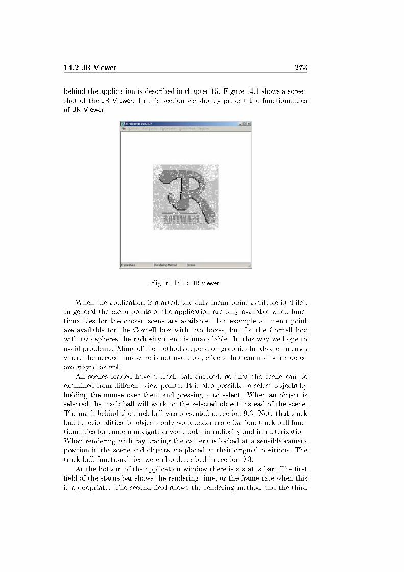
14.2 JR Viewer 273behind the appli ation is des ribed in hapter 15. Figure 14.1 shows a s reenshot of the JR Viewer. In this se tion we shortly present the fun tionalitiesof JR Viewer.

Figure 14.1: JR Viewer.When the appli ation is started, the only menu point available is �File�.In general the menu points of the appli ation are only available when fun -tionalities for the hosen s ene are available. For example all menu pointare available for the Cornell box with two boxes, but for the Cornell boxwith two spheres the radiosity menu is unavailable. In this way we hope toavoid problems. Many of the methods depend on graphi s hardware, in aseswhere the needed hardware is not available, e�e ts that an not be renderedare grayed as well.All s enes loaded have a tra k ball enabled, so that the s ene an beexamined from di�erent view points. It is also possible to sele t obje ts byholding the mouse over them and pressing P to sele t. When an obje t issele ted the tra k ball will work on the sele ted obje t instead of the s ene.The math behind the tra k ball was presented in se tion 9.3. Note that tra kball fun tionalities for obje ts only work under rasterization, tra k ball fun -tionalities for amera navigation work both in radiosity and in rasterization.When rendering with ray tra ing the amera is lo ked at a sensible ameraposition in the s ene and obje ts are pla ed at their original positions. Thetra k ball fun tionalities were also des ribed in se tion 9.3.At the bottom of the appli ation window there is a status bar. The �rst�eld of the status bar shows the rendering time, or the frame rate when thisis appropriate. The se ond �eld shows the rendering method and the third

274 Graphi al User Interfa e�eld (in general) shows the urrent s ene.In the following we will present the dropdown menus one by one.The File Menu

Figure 14.2: The File menu.In the File menu, see �gure 14.2, we �nd all the available test s enes. Wehave hosen to make the s enes des ribed in the previous se tion dire tlyavailable1 so that a user more easily an make sample images at all times.Beneath these test s enes we have made an option for import of an arbitraryX3D s ene. For reasons mentioned in the previous se tion, it is only possibleto use the rasterization menu with su h a s ene.When a new s ene is loaded all settings are reset. This means that nomatter the settings that were sele ted for the last s ene and the renderingmethod that was used, all settings will we desele ted and the rendering ofthe s ene will appear as plane OpenGL rasterization when a new s ene isloaded.Two setting dialogs are also available in the �le menu. There is a set-ting dialog for s ene parameters and a setting dialog for obje t parameters.The s ene parameter settings dialog is only available when a s ene has beenopened and the obje t parameter settings dialog is only available when anobje t has been pi ked. Figure 14.3 shows the s ene parameters dialog and�gure 14.4 shows the obje t parameters dialog. Parameter an be set toexa t values by the text �elds. Obje t parameters have asso iated slide barsfor intera tive hanges to the parameters. Otherwise parameters should be1Some of the s enes may be grayed be ause we did not �nd time to insert them in the�nal frame work.

14.2 JR Viewer 275

Figure 14.3: S reen shot of the s ene parameter dialog.updated by the urrent number when <RETURN> is pressed. To leave the text�elds without updating <ESC> should be pressed. Unfortunately we have nothad the time to ouple the parameter settings to our render engine, but thewindows exist for future use.Sin e the parameter settings still do not quite ouple to the render engine,they will not be des ribed any further at this point.Using the last �le menu option we an exit the appli ation.The Radiosity MenuThrough the radiosity menu (�gure 14.5) we an sele t a few radiosity ren-dering methods. The radiosity menu will only work with two s enes: Theempty Cornell box and the Cornell box with two boxes. The radiosity ren-dering is merely present in this appli ation for omparison with the otherimplemented methods.As des ribed in se tion 13.1, we an hose between two di�erent methodsfor radiosity solutions: The analyti al method and the hemi ube method.Also available is a view of the pat hes used in the al ulations.Camera movement is possible after the radiosity solution has been al- ulated. Obje ts an not be moved without re al ulation of the radiositysolution, therefore obje t sele tion has been disabled under the radiositymenu.

276 Graphi al User Interfa e

Figure 14.4: The obje t parameter dialog. Figure 14.5: The Radiosity menu.The Ray Tra ing MenuThe ray tra ing menu (�gure 14.6) enables ray tra ing of the simple s enes.Di�erent rendering equation terms, shading methods, and shadow methods an be applied in the ray tra ing pro ess. These are hosen from the menu.The menu presents a number of e�e ts that an be toggled on or o� witha mouse li k. Some e�e ts rule out others, for example it makes no senseto render both hard and soft shadows, hen e if soft shadows are sele ted,hard shadows are automati ally desele ted. Setting points that rule ea hother out are isolated from the other points by lines (the �rst points do notrule out ea h other). Some menu points have no e�e t on some s enes, forexample it gives no e�e t to enable spe ular re ursions if none of the obje tsin the s ene are spe ular. When appropriate settings have been sele ted themenu option �Go. . . � should be sele ted for ray tra ing of the s ene.Sin e no intera tivity is available after ray tra ing the resulting image isstret hed over a quad as a texture in order to make it s alable. The original

14.2 JR Viewer 277

Figure 14.6: The Ray Tra ing menu.texture is 512x512 pixels. In ray tra ing we have hosen to have the amera�xed at a sensible position in the s ene. The s enes in whi h the ray tra ingmenu is available were pointed out in the previous se tion.In hapter 13 we des ribed the di�erent rendering methods that are avail-able with pointers ba k through the report. In the following we will shortlydes ribe the di�erent menu options for ray tra ing and photon mapping:� �Ambient light� adds a onstant ambient term to the rendering equa-tion in order to give a rude simulation of multiple di�use re�e tions.� �Spe ular re ursions� spawn re�e ted and refra ted rays if the materialparameters indi ate that it is ne essary.� �Causti s� estimate the austi s term of the rendering equation by useof a austi s photon map.� �Hardware optimized� toggles al ulation of the �rst interse tion inhardware using the idea des ribed in se tion 11.7.� �Phong shading� uses Phong shading for the dire t illumination term.Phong shading desele ts the other available shading options.� �Blinn-Phong shading� uses Blinn-Phong shading for the dire t illumi-nation term and desele ts the other available shading options.

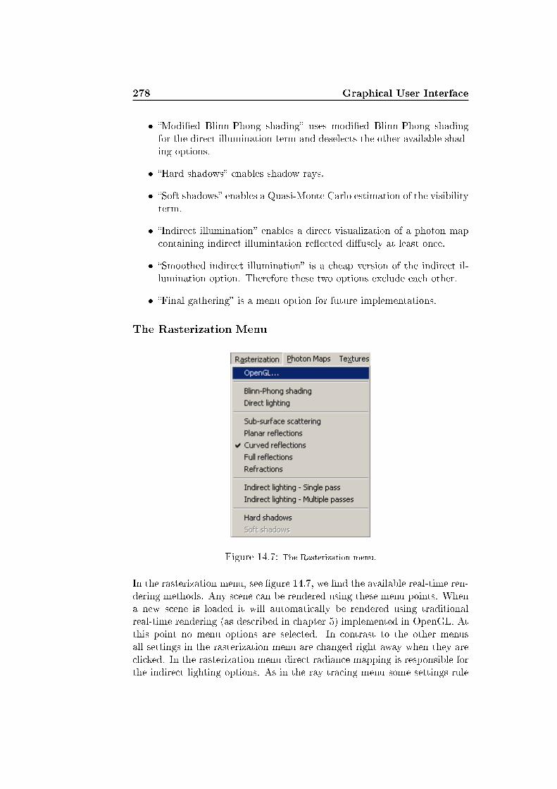
278 Graphi al User Interfa e� �Modi�ed Blinn-Phong shading� uses modi�ed Blinn-Phong shadingfor the dire t illumination term and desele ts the other available shad-ing options.� �Hard shadows� enables shadow rays.� �Soft shadows� enables a Quasi-Monte Carlo estimation of the visibilityterm.� �Indire t illumination� enables a dire t visualization of a photon map ontaining indire t illumintation re�e ted di�usely at least on e.� �Smoothed indire t illumination� is a heap version of the indire t il-lumination option. Therefore these two options ex lude ea h other.� �Final gathering� is a menu option for future implementations.The Rasterization Menu

Figure 14.7: The Rasterization menu.In the rasterization menu, see �gure 14.7, we �nd the available real-time ren-dering methods. Any s ene an be rendered using these menu points. Whena new s ene is loaded it will automati ally be rendered using traditionalreal-time rendering (as des ribed in hapter 5) implemented in OpenGL. Atthis point no menu options are sele ted. In ontrast to the other menusall settings in the rasterization menu are hanged right away when they are li ked. In the rasterization menu dire t radian e mapping is responsible forthe indire t lighting options. As in the ray tra ing menu some settings rule

14.2 JR Viewer 279out others and some settings are irrelevant for some s enes. To shift to ras-tization after having used another rendering method (su h as ray tra ing),sele t the top menu option �OpenGL. . . �.The following list des ribes the di�erent options one by one.� �Blinn-Phong shading� swit hes from the standard Phong highlightingto Blinn-Phong shading implemented in a fragment shader.� �Dire t lighting� enables an analyti al solution of the dire t illumina-tion term whi h is des ribed in hapter 12. The Blinn-Phong shadingand the dire t lighting options both simulate the dire t illuminationterm, and therefore they ex lude ea h other.� �Sub-surfa e s attering� enables our rude simulation of subsurfa es attering as des ribed in hapter 12.� �Planar re�e tions� allows real-time planar re�e tions.� �Curved re�e tions� use environment mapping for real-time urved re-�e tions.� �Full re�e tions� makes sure that the orre t lighting is used in the urved re�e tions and it also makes the urved re�e tions re ursive.� �Refra tions� enables the spe ialized refra tions des ribed in se tion13.2.� �Indire t lighting - single pass� enables dire t radian e mapping re- al ulated for ea h frame.� �Indire t lighting - multiple passes� al ulates dire t radian e mappingover several frames. This implementation exists in an early version ofthe appli ation, but unfortunately we did not �nd the time to in or-porate it in the urrent frame work.� �Hard shadows� enables shadow volumes.� �Soft shadows� are in the future works department.The Photon Maps MenuSeveral e�e ts under the ray tra ing menu uses photon mapping. To give anidea of the te hnology behind the s ene, we have made a visualization of thedi�erent photon maps available in the Photon Maps menu, see �gure 14.8.Any ombination of photon maps is allowed. The following photon maps areavailable:� �Dire t light� shows the dire t photons, whi h are photons stored whenthe surfa e interse ted �rst is a di�use surfa e.

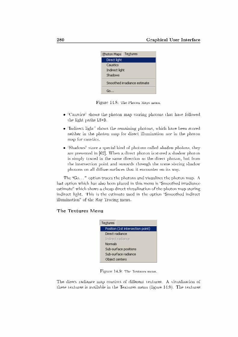
280 Graphi al User Interfa e Figure 14.8: The Photon Maps menu.� �Causti s� shows the photon map storing photons that have followedthe light paths LS+D.� �Indire t light� shows the remaining photons, whi h have been storedneither in the photon map for dire t illumination nor in the photonmap for austi s.� �Shadows� store a spe ial kind of photons alled shadow photons, theyare presented in [62℄. When a dire t photon is stored a shadow photonis simply tra ed in the same dire tion as the dire t photon, but fromthe interse tion point and onwards through the s ene storing shadowphotons on all di�use surfa es that it en ounter on its way.The �Go. . . � option tra es the photons and visualizes the photon map. Alast option whi h has also been pla ed in this menu is �Smoothed irradian eestimate� whi h shows a heap dire t visualization of the photon map storingindire t light. This is the estimate used in the option �Smoothed indire tillumination� of the Ray Tra ing menu.The Textures Menu Figure 14.9: The Textures menu.The dire t radian e map onsists of di�erent textures. A visualization ofthese textures is available in the Textures menu (�gure 14.9). The textures

14.2 JR Viewer 281are presented in the following list. All the textures are used for the dire tradian e mapping method and are not applied as olor textures anywhere inthe s ene.� �Position� is a texture providing the �rst interse tion points seen fromthe light sour e.� �Dire t radian e� gives the dire t illumination stored in the dire t ra-dian e map.� �Normals� is a texture providing the normals at ea h interse tion pointseen from the light sour e.� �Sub-surfa e positions� orresponds to the Position texture ex ept itpi tures interse tion points found inside translu ent obje ts.� �Sub-surfa e radian e� �nds the radian e rea hing the points givenin the Sub-surfa e positions texture after attenuation while travelingthrough the translu ent obje t.� �Obje t enters� provides the obje t enters a ording to whi h thesubsurfa e s attering is sampled. This texture is not absolutely ne -essary sin e the obje t enters an be provided to the dire t radian emapping method as uniform variables.This on ludes the presentation of our graphi al user interfa e (GUI). Ween ourage use of the appli ation itself whi h is available on the CD-ROMa ompanying this report, see appendix A. In the following hapter we willdes ribe the stru ture of the implementation behind the GUI.

282 Graphi al User Interfa e

Chapter 15Implementation

Progress lies not in enhan ing what is, but in advan ing towardwhat will be.Kahlil Gibran (1883-1931): A Handful of Sand on the Shore

284 ImplementationMu h implementation has been done during this proje t, in this hapter wepresent the design of our �nal appli ation, whi h is a essed through theGUI des ribed in the previous hapter. Implementation has been done usingthe following freely available tools:� OpenGL open sour e graphi s library (in luding extensions)� BCC55 Borland C++ ommandline ompiler version 5.5� makegen for reating make�les� expat for XML parsing� GLUT OpenGL Utility Toolkit� CG C for Graphi s� Python for export s riptingThe purpose of this hapter is to provide the reader with an overviewof the program parts. Thereby we hope to reveal all the aspe ts of theappli ation. After giving an overview the hapter will present ea h programpart in a more detailed manner. The a tual ode will not be presented inthis hapter but is available on the atta hed CD-ROM, see appendix A.Se tion 15.1 des ribes the overall program stru ture. After that the se -tions of this hapter are divided into di�erent kinds of menu options. Se tion15.2 des ribes status options, se tion 15.3 des ribes render options, and se -tion 15.4 des ribes s ene options. Finally se tion 15.5 gives a design diagramof the render engine, whi h is used for several di�erent menu options.15.1 Program Stru tureThrough the JR Viewer we give a ess to the di�erent rendering methods thathave been implemented. The sour e ode for the program is divided intodi�erent libraries ea h treating its own part of the proje t. Ea h sour e �lestarting with a apital letter implements an obje t, otherwise it implementsa tool for the obje ts or the appli ation in general. The main �le (whi his alled main. pp) ontains the WinMain fun tion for the JR Viewer. Thestru ture of the program is quite similar to the stru ture of the sour e �lesand libraries, whi h are divided mainly a ording to the menus in the GUI.Appendix C shows the stru ture of the sour e �les and the libraries for theprogram. The stru ture of the program is presened in �gure 15.1.There are three ore modules in for the appli ation. The WinMain fun -tion pla ed in the main �le (main. pp), whi h ontrols the GUI, and therebyalso the appli ation. The render engine (pla ed in the engine library, see app.C) where all the geometry is ontained and where the most basi rendering

15.1 Program Stru ture 285

Math Engine

Trackball

B-Mesh

File

Logo

Radiosity

02561 Exercise

Ray Tracing

Photon Maps

Rasterization

Textures

Render Engine

JR VIEWER

WIN Main

Figure 15.1: The program stru ture. The names in the boxes refer partly to the menuoptions, partly to the libraries and partly to ontrolling �les.is done. 02561 Exer ise (from the radiosity library) that takes are of theradiosity rendering.The rest of the boxes inside the JR Viewer ontainer in �gure 15.1 ea hrefer to a menu of the appli ation ex ept for the logo box whi h is the logoused as the starting pi ture. The boxes outside the JR Viewer ontainer aregeneral tools that an be used by all of the �les in the JR Viewer.The JR Viewer is a MS Windows appli ation. Windows is a multitaskingoperating system; this means that multiple appli ations or programs an runat the same time in what is alled threads [47℄. A great tutorial for gettingstarted with windows programming an be found at [83℄.To enable a tions, messages are sent from windows to the appli ation,it is then up to the appli ation to respond to these messages. The fun tionhandling messages is the allba k fun tion. The allba k fun tion is merelya long list of ases with a ase for ea h relevant message (irrelevant messagesare simply ignored).There are a number of allba k fun tions in the appli ation. The most

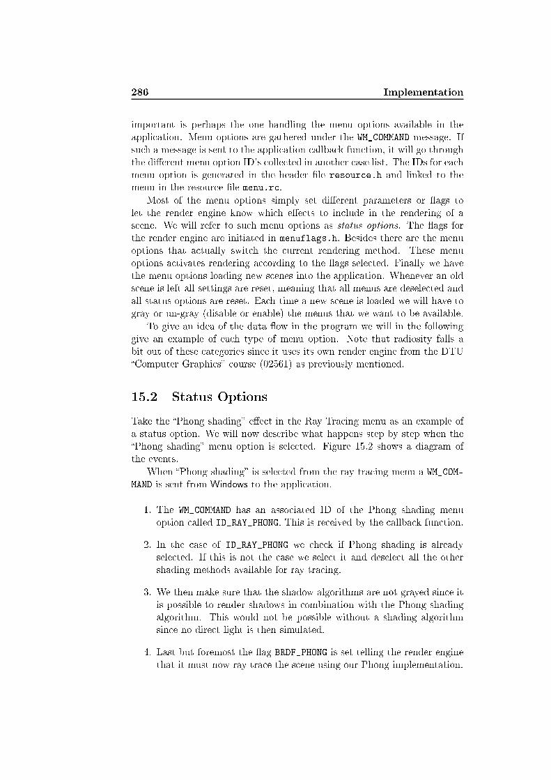
286 Implementationimportant is perhaps the one handling the menu options available in theappli ation. Menu options are gathered under the WM_COMMAND message. Ifsu h a message is sent to the appli ation allba k fun tion, it will go throughthe di�erent menu option ID's olle ted in another ase list. The IDs for ea hmenu option is generated in the header �le resour e.h and linked to themenu in the resour e �le menu.r .Most of the menu options simply set di�erent parameters or �ags tolet the render engine know whi h e�e ts to in lude in the rendering of as ene. We will refer to su h menu options as status options. The �ags forthe render engine are initiated in menuflags.h. Besides there are the menuoptions that a tually swit h the urrent rendering method. These menuoptions a tivates rendering a ording to the �ags sele ted. Finally we havethe menu options loading new s enes into the appli ation. Whenever an olds ene is left all settings are reset, meaning that all menus are desele ted andall status options are reset. Ea h time a new s ene is loaded we will have togray or un-gray (disable or enable) the menus that we want to be available.To give an idea of the data �ow in the program we will in the followinggive an example of ea h type of menu option. Note that radiosity falls abit out of these ategories sin e it uses its own render engine from the DTU�Computer Graphi s� ourse (02561) as previously mentioned.15.2 Status OptionsTake the �Phong shading� e�e t in the Ray Tra ing menu as an example ofa status option. We will now des ribe what happens step by step when the�Phong shading� menu option is sele ted. Figure 15.2 shows a diagram ofthe events.When �Phong shading� is sele ted from the ray tra ing menu a WM_COM-MAND is sent from Windows to the appli ation.1. The WM_COMMAND has an asso iated ID of the Phong shading menuoption alled ID_RAY_PHONG. This is re eived by the allba k fun tion.2. In the ase of ID_RAY_PHONG we he k if Phong shading is alreadysele ted. If this is not the ase we sele t it and desele t all the othershading methods available for ray tra ing.3. We then make sure that the shadow algorithms are not grayed sin e itis possible to render shadows in ombination with the Phong shadingalgorithm. This would not be possible without a shading algorithmsin e no dire t light is then simulated.4. Last but foremost the �ag BRDF_PHONG is set telling the render enginethat it must now ray tra e the s ene using our Phong implementation.

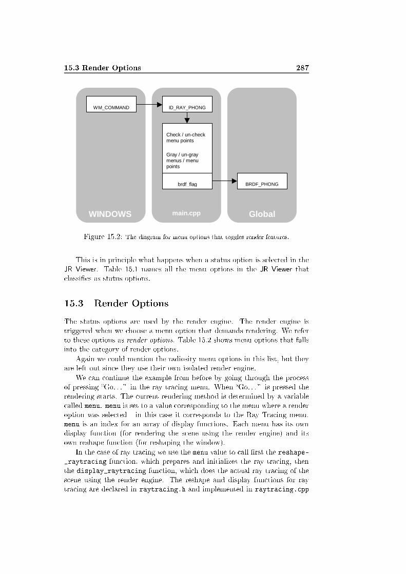
15.3 Render Options 287

WM_COMMAND ID_RAY_PHONG

Check / un-check menu points

Gray / un-gray menus / menu points

brdf_flag BRDF_PHONG

WINDOWS main.cpp Global Figure 15.2: The diagram for menu options that toggles render features.This is in prin iple what happens when a status option is sele ted in theJR Viewer. Table 15.1 names all the menu options in the JR Viewer that lassi�es as status options.15.3 Render OptionsThe status options are used by the render engine. The render engine istriggered when we hoose a menu option that demands rendering. We referto these options as render options. Table 15.2 shows menu options that fallsinto the ategory of render options.Again we ould mention the radiosity menu options in this list, but theyare left out sin e they use their own isolated render engine.We an ontinue the example from before by going through the pro essof pressing �Go. . . � in the ray tra ing menu. When �Go. . . � is pressed therendering starts. The urrent rendering method is determined by a variable alled menu. menu is set to a value orresponding to the menu where a renderoption was sele ted - in this ase it orresponds to the Ray Tra ing menu.menu is an index for an array of display fun tions. Ea h menu has its owndisplay fun tion (for rendering the s ene using the render engine) and itsown reshape fun tion (for reshaping the window).In the ase of ray tra ing we use the menu value to all �rst the reshape-_raytra ing fun tion, whi h prepares and initializes the ray tra ing, thenthe display_raytra ing fun tion, whi h does the a tual ray tra ing of thes ene using the render engine. The reshape and display fun tions for raytra ing are de lared in raytra ing.h and implemented in raytra ing. pp

288 ImplementationRay Tra ing !Ambient LightRay Tra ing !Spe ular Re ursionsRay Tra ing !Causti sRay Tra ing !Hardware optimizedRay Tra ing !Phong shadingRay Tra ing !Blinn-Phong shadingRay Tra ing !Modi�ed Blinn-Phong shadingRay Tra ing !Hard shadowsRay Tra ing !Soft shadowsRay Tra ing !Indire t illuminationRay Tra ing !Smoothed indire t illuminationRasterization!Blinn-Phong shadingRasterization!Dire t lightingRasterization!Sub-surfa e s atteringRasterization!Planar re�e tionsRasterization!Curved re�e tionsRasterization!Full re�e tionsRasterization!Refra tionsRasterization!Indire t light - single passRasterization!Hard shadowsRasterization!Soft shadowsPhoton Maps!Dire t lightPhoton Maps!Causti sPhoton Maps!Indire t lightPhoton Maps!ShadowsPhoton Maps!Smoothed irradian e estimatesTable 15.1: A list of all the status options in the JR Viewer, that is, all the menu optionsthat an be sele ted or desele ted with in�uen e on the rendering method.Ray tra ing !Go. . .Rasterization!OpenGL. . .Photon Maps!Go. . .Textures !PositionTextures !Dire t radian eTextures !NormalsTextures !Sub-surfa e positionsTextures !Sub-surfa e radian eTextures !Obje t entersTable 15.2: Menu options that triggers the rendering engine.

15.4 S ene Options 289(in the raytra ing library). The render engine makes use of the �ags set bythe status options, we will return to this in a little while. reshape_raytra -ing is alled on e when �Go. . . � is pressed, and it is only alled subsequentlyif the window is reshaped. display_raytra ing is alled in the main loopwhenever the appli ation has nothing else to deal with.The pro ess is des ribed in the following sequen e and illustrated in �gure15.3. In other words the following is what happens when WM_COMMAND is alledwith ID_RAY_GO.1. The WM_COMMAND has an asso iated ID of the �Go. . . � menu option alled ID_RAY_GO. This is re eived by the allba k fun tion.2. A message is sent to the status bar telling that ray tra ing is now the urrent rendering method.3. A shade option is al ulated using the status �ags. It is used formaterial al ulation purposes in the render engine.4. The menu parameter is set to a value orresponding to the Ray Tra ingmenu.5. Initialize OpenGL for rendering. This is always done when a renderoption is sele ted to make sure that we start from s rat h.6. reshape_raytra ing is alled for initialization of the ray tra ing.7. Sin e the menu variable has been altered the main loop will now allthe display_raytra ing whenever the appli ation is idle. Thereforethe display_raytra ing fun tion arries out the ray tra ing of thes ene using the render engine.This example is for ray tra ing, but the pro ess is nearly the same nomatter what rendering method we hoose. In the ase of radiosity thoughall pro essing is arried out in the separate renderer for radiosity.15.4 S ene OptionsTo make all this useful we need something to render. We load s enes throughthe �le menu. When a �le is loaded all previous menu settings are reset. News enes are always rendered using the OpenGL menu option under rasteriza-tion as this is available for all s enes. Table 15.3 ontains all menu option inthis ategory. We all those menu options s ene options.As an example of loading a s ene we look loser at the Cornell box on-taining two spheres. The ID for this s ene is ID_FILE_TWOSPHERECB, whenthis ase entry is triggered the old world will be erased and the fun tion

290 Implementation

WM_COMMAND

WINDOWS Send message to status bar

ID_RAY_GO

Global

BRDF_PHONG

Shade option calculation

Set menu value

main.cpp

shade_option

Main loop display

Function call

raytracing.cpp

Render engine

reshape_raytracing

display_raytracing

Figure 15.3: Rendering using the JR Viewer.File!Cornell box - EmptyFile!Cornell box - Two boxesFile!Cornell box - Two spheresFile!Cornell box - Sphere and boxFile!Cornell box - OrbFile!Cornell box - ArthurFile!Cave s eneFile!Load s ene. . . Table 15.3: The s ene options.

15.5 The Render Engine 291 ornell_2spheres will load the new s ene into a new world. ornell-_2spheres is de lared in file.h and implemented in file. pp ( ontainedin the �le library). This fun tion loads a Cornell box ontaining two spheresinto the appli ation. After this the network of angular visibility between theobje ts ( f. se . 11.1) is initialized. Then di�erent relevant menus and menuoptions are un-grayed as all menus are grayed and all settings are reset whena new s ene is to be loaded. Finally we send a message to the status bar withthe name of the s ene and a boolean variable is set whi h indi ates whetherthe loading of the s ene was su essful or not. If this �ag is set false thestart up logo will be loaded instead of the hosen s ene.The following list des ribes the pro edure step by step and �gure 15.4shows a diagram of what happens.1. The WM_COMMAND has an asso iated ID of the Cornell box - two spheresmenu option alled ID_FILE_TWOSPHERECB. This is re eived by the all-ba k fun tion.2. The fun tion ornell_2spheres is alled for loading of a s ene on-taining two spheres in a Cornell box.3. Angular visibility network is initialized in the World obje t of the ren-der engine.4. All menus ex ept radiosity, whi h is not available for this s ene, area tivated.5. As the s ene ontain a refra tive obje t austi menu options are en-abled in the ray tra ing and photon maps menus. S ene parameterdialog menu option is un-grayed as well, sin e a s ene is now available.6. The s ene name is sent to the status bar.7. It is reported whether the loading was su essful or not.8. If the load was su essful OpenGL rendering is initialized and the menuvariable is set to the rasterization menu.15.5 The Render EngineThe above text and diagrams should explain the di�erent aspe ts of theimplemented appli ation. One important step is still missing though; therendering pro ess arried out by the render engine. A design diagram of therender engine is presented in �gure 15.5When a new s ene is loaded as des ribed above, a new World obje tholding s ene geometry, material, and light sour es is reated for the render

292 Implementation

WM_COMMAND

WINDOWS

ID_FILE_ TWOSPHERECB

Render Engine

Load scene

main.cpp

Initialize network

file.cpp

cornell_2spheres

Check / un-check menu points

Gray / un-gray menus / menu points

Send message to status bar

Report load successful

Figure 15.4: The pro ess of loading a s ene.

15.5 The Render Engine 293

Ray

Tra

cin

g

World Object Selection Correction

Photon Emission

Photon Map

Geometry

Ray Tracing

Rasterization

Material Shading

Render Engine

Ph

oto

n M

aps

Ras

teri

zati

on

Tex

ture

s

Global

Figure 15.5: A design diagram for the render engine.

294 Implementationengine. Depending on the rendering method hosen by a render option, therender engine will be invoked di�erently. As indi ated in �gure 15.5 raytra ing will tra e single rays through the s ene by interse tion al ulations,while rasterization will rasterize the s ene geometry on e. The shading boxin �gure 15.5 should be regarded di�erently depending on the renderingmethod.Ray tra ing will shade ea h ray independently by use of the render engine.To speed up the ray tra ing pro ess by avoiding time onsuming if-senten esin the main loop of the ray tra ing algorithm, we have hosen to reate fun -tions for ea h ombination of sele ted status options. The di�erent fun tionsare assembled in an array and the fun tion to use is by shade_option, whi has previously mentioned was al ulated using the di�erent �ags set in theray tra ing menu. The array of di�erent shading fun tions is implementedin Material.h and in Material. pp.Rasterization will rather use the render engine to obtain geometry, mate-rial, and light settings before rasterizing the s ene using vertex and fragmentprograms. The shading box ould therefore be regarded as a fragment pro-gram in the rasterization ase. Textures are reated using the render enginein the same way as when rasterization is done. Where we in the rasterizationapproa h use the textures for later passes, we display them dire tly when therender options in the Textures menu have been hosen.Photon mapping is oupled to the ray tra ing pro edure as indi atedby the stippled route through the diagram in �gure 15.5. If we store thephotons, whi h are stored in a photon map, in an OpenGL display list aswell while emitting photons. We an visualize the photon maps as indi atedby the green arrows in the diagram.This hapter has des ribed the super� ial �ow of data in our program.For exa t implementation details we refer to the sour e ode on the atta hedCD-ROM (see appendix A). This on ludes the des ription of our experi-ments, ideas, and implementations. What remains are some on lusive wordsgiven in part IV.

Part IVCon lusions

Chapter 16Dis ussion

. . . as we know, there are known knowns; there are things we knowwe know. We also know there are known unknowns; that is to saywe know there are some things we do not know. But there arealso unknown unknowns - the ones we don't know we don't know.Donald Rumsfeld, US Se retary of Defen e (2003)

298 Dis ussionOne purpose of this thesis was to move realisti image synthesis loser to real-time omputer graphi s. After thorough studies of illumination methods andhow to repli ate the intera tion of light with matter we set out to generateour own methods for simulation of global illumination e�e ts in real-time. Anumber of ideas appeared and one was hosen as the most promising. Thisidea, referred to as dire t radian e mapping, has been dis ussed in detail in hapter 12.Another obje tive was to produ e the entire work �ow from the reationof s ene meshes to the illumination of them in real-time, using a dynami appli ation. This obje tive has been obliged through revision of Blenderand the building of a demonstration appli ation (the JR Viewer). The fun -tionalities of Blender were des ribed in hapter 10 and the demonstrationappli ation was presented in hapter 14.In this hapter we will on entrate on the parts that yet remains tobe dis ussed in this report. Se tion 16.1 will address future aspe ts of theproje t and what we would have done if more time had been available. Theappli abilities of the proje t ideas, results, and experiments will be dis ussedin se tion 16.2.16.1 Future experimentsThe idea of dire t radian e mapping ame to us at a fairly late time dur-ing the proje t, sin e it was the out ome of in-depth theoreti al studies ofglobal illumination and the pra ti al angle gained through implementationof di�erent illumination methods. The same studies and implementationsformed a number of other ideas as well presented in hapter 11. It ouldbe interesting to pursue some of the ideas a little further. The more on- eptual ideas su h as the topologi al network des ribed in se tion 11.2 andthe multi-agent approa h des ribed in se tion 11.4 are the ideas that we �ndmost interesting for future development. These two approa hes ould be ombined and perhaps they may even be useful in a ombination with dire tradian e mapping.A modest idea su h as angular visibility, des ribed in se tion 11.1, anin fa t �nd many small appli abilities here and there. Re all, for example,that we assume in our dire t illumination al ulation that light sour es arevery distant from the s ene. This means that the angle used for the osineterm in the radian e al ulation is found a ording to the dire tion towardsthe enter of the light sour e. The result is that the side of the large box inthe Cornell box (see �g. 12.2) is entirely bla k though the area light sour ewould in fa t illuminate it from a part of its area. The angular visibility ould be used to �nd the size of this area and thereby a better estimate ofthe dire t illumination resulting from an isotropi area light approximatedby a point light would be available.

16.1 Future experiments 299Dire t radian e mapping in itself still ontains unexplored territories.There are many interesting expansions and experiments that ould be workedwith. The method still has many �aws and ideas for removing some of theseare presented in hapter 12. To better ompare the on ept of dire t radian emapping with ordinary global illumination methods and to generate a proofof on ept implementation, it ould also be interesting to implement the on eptual method (se . 12.1) in software with an a tual network for lightpropagation instead of the instru tion limited implementation that we havenow on the GPU.In the nearest future a trimming of the method would be appropriateremoving some of the most signi� ant drawba ks like �i kering and overex-posure of indire t illumination and missing indire t shadows, some proposalsfor their solutions were given in hapter 12.New GPUs, already available at the market, have fun tionalities whi hour method an bene�t from signi� antly. Important fun tionalities of 6thgeneration GPUs are the feature alled render to multiple targets, whi hwould make the many passes for rendering low-resolution texture a singlepass or two only, and true looping whi h an signi� antly improve on thepro essing time onsumed by our fragment programs for indire t illumina-tion. Render-to-texture is another improvement that we even ould havetried on the hardware we urrently have available. Unfortunately we did not�nd time for this. Wishful thinking from our side is to hope for new GPUswith a mipmapping instru tion available in fragment programs.The demonstration appli ation of the proje t also has its limitations. Asthe basi appli ation is merely made to demonstrate our proje t a omplish-ments and to show that we are able to use s enes that we have modeledexternally in a modeling tool, it is important to make the export and imports ripts more robust and ooperative. This is ru ial for using our implemen-tations in other onne tions. Therefore a future assignment is to improve onthose.A number of global illumination algorithms have been implemented for omparison purposes. These implementations have also been important inour learning pro ess and therefore more su h implementations are wel omein the future.For omparison purposes as well, it ould be enlightening to implementsome of the ompetitive methods des ribed in hapter 6. As mentioned inse tion 12.4 some of the ideas used in these methods might also be ombinedwith dire t radian e mapping. Implementing them would therefore be anopportunity to study the method in details and �nd out how ombinations ould be arried out best.In hapter 12 we mention and idea of an environment map for ea h obje tin the s ene. We �nd that this idea, though dependent on the number ofobje ts in the s ene, ould be very interesting to pursue. It seems as a good hoi e for al ulation of multiple boun es in the estimate of di�usely re�e ted

300 Dis ussionindire t illumination.Looking at the in orre t bright spots in �gure 12.6, we may shortly bringup an old-timer - Lambert after whom Lambertian surfa es are named. Inhis Photometria (1760) Lambert presented the ��ve-times� rule of thumb [2,p. 187℄:If the distan e from the light sour e is �ve times or more thatof the light's width, then the inverse square law is a reasonableapproximation and so an be used. Closer than this and thesolid angle the light overs will vary noti eably di�erent from aninverse square relationship.Thinking of the sample points in our s ene as light sour es of a size equalto eg. AM=N , where N is the number of sample points, we may be able toavoid the bright spots by Lambert's ��ve-times� rule of thumb.Though mipmaps are dis ussed here and there in the pre eding hapters,we think that many opportunities yet lie in mipmapping ombined withdire t radian e mapping. An idea is to use a mipmap for the light sour eimages. Then we should use the level in the mipmap that orresponds bestto the number of sample points that we an a�ord. This might make dire tradian e mapping mu h more robust. Another thing is that we ould ombineshadow maps with this idea. Then the shadow map an use a high resolutiontexture while DRM uses a low resolution texture at a higher level in themipmap. For this to work, it is ne essary that we must be able to hoosespe i� ally in the fragment program, whi h level in the mipmap that wewant to use. This fun tionality is fortunately available on modern graphi shardware.With respe t to modeling it would be ni e to examine the Blender Renderin-depth. Then we ould ompare Blender renders to our own renderings.Also we ould ompare our real-time results to the real-time results availablethrough Blender's game engine.As a development of our work �ow on ept we would also like to developthe JR Viewer further by adding di�erent features ontinually. Examples offeatures are: Conne tion of several s enes, animations and dynami lighte�e ts, and maybe even a physi s engine. By adding su h features we wouldgradually ome loser to a truly dynami appli ation and eventually we wouldhave all the tools needed for a free of harge game development platform.This se tion holds many ideas for future experiments and more ouldprobably be found. For example, we ould work on some of the subje tsthat have largely been negle ted in this proje t; S ene graphs, spatial datastru tures, anti-aliasing, real-time soft shadows, et . This on ludes ourdis ussion on future work. In the following se tion we will dis uss the appli- abilities of this proje t.

16.2 Appli ability 30116.2 Appli abilityDire t radian e mapping in its urrent form is not su� ient for use in om-mer ial appli ations it is still on an experimental stage. To make it suitablefor ommer ial appli ations there are many problems that must be dealtwith. First of all the frame rate must be higher and the �i kering andoverexposure of indire t illumination must be orre ted. With more timeinvested in improvements of the method and the frequently in reasing speedof graphi s hardware we believe that there is hope for dire t radian e map-ping. Still the method very mu h depends on hardware and sin e it maytake a while before GPUs be ome fast enough for the method, it will takeeven longer before the average onsumer will have su h hardware available.One thing speaking in favor of dire t radian e mapping, in this respe t, isthat it an be applied at di�erent levels of omplexity (the sample points an be adjusted or spread over several frames).One of the goals of this proje t was to reate a platform for developingreal-time dynami appli ations su h as omputer games. During the proje twe have managed to establish the beginning of a free of harge game de-velopment platform. This is done using various sour es in luding our ownsoftware. All tools that have been used, from ompiler to modeling program,are free of harge and available on the internet. Although we have not re-ated a omplete game we have taken the �rst small step by generating anappli ation able to present our own modeled s enes using our own renderengine. Of ourse there is a long way to a �nished produ t, but we believe tohave provided a proof of on ept showing that it is possible to get far withlittle expenses on software.The appli ation that we have built is used mainly for presentation pur-poses and for omparing di�erent rendering methods. As it is possible to loadarbitrary s enes in X3D format others an use the appli ation for demon-stration purposes as well. The appli ation an of ourse be used by othersto ompare their rendering methods with the traditional methods as well asours.In the �nal hapter we will sum up on the report and give our �nalremarks.

302 Dis ussion

Chapter 17Con lusion

We have a habit in writing arti les published in s ienti� journalsto make the work as �nished as possible, to over up all the tra ks,to not worry about blind alleys or des ribe how you had the wrongidea at �rst, and so on. So there isn't any pla e to publish, in adigni�ed manner, what you a tually did in order to get to do thework. Ri hard Bu kminster Fuller (1895-1983)

304 Con lusionThis thesis en ompasses two main obje tives. First, we wanted to explorehow lose we ould bring realisti image synthesis to real-time exe utionrates, and se ondly, we wanted to make a platform for development of real-time appli ations.The report is divided into four parts. The �rst part mainly serves the �rstobje tive, the se ond part mainly serves the se ond obje tive, and part IIIserves both obje tives by a presentation of the ideas, results, and experimentsthat we have had during this proje t. Part IV (this part) dis usses and on ludes the report.The �rst part builds the theoreti foundation for the rest of the proje t.The hapters of this part have served several purposes. Chapter 2, for exam-ple, presents an array-based math engine whi h an be used for an e� ientimplementation of ve tor and matrix math. Chapter 3 is important in or-der to understand the fundamental illumination model behind the globalillumination that we would like to simulate in real-time. Having a goodunderstanding of the global illumination model enable us to dis over theabilities and limitations of a method before taking it too far.The theoreti al angle to a subje t is rarely enough to give a full under-standing. Therefore we introdu ed di�erent traditional methods for bothrealisti image synthesis ( hapter 4) and real-time rendering ( hapter 5).Whi h parts of these methods that we have implemented are des ribed in hapter 13.During the implementation of these methods we ame up with severalideas, some for improvement of spe i� methods, others for more on eptualapproa hes to rendering of global illumination. The ideas are des ribed in hapter 11 and listed below.1. Angular visibility between axis aligned bounding boxes (AABBs) forfewer interse tion tests in ray tra ing.2. A topologi al network for radian e transfer between obje ts.3. Displa ement mapping for fast ray/obje t interse tion.4. A multi-agent approa h to global illumination, where ea h obje t is anautonomous agent ontrolling its own shade.5. An `atmosphere' to limit the in�uen e of ea h obje t in global illumi-nation.6. A line-of-sight algorithm for fewer interse tion tests in ray tra ing.7. Gouraud interpolation of the �rst interse tion point. A rasterizationapproa h to the �rst level of the ray tra ing algorithm.8. Single pixel images ea h representing a ray. An attempt to let rasteri-zation do full re ursive ray tra ing.

305A ombination of the di�erent traditional methods we had implementedand the ideas in hapter 11, ended up in a spe i� idea alled dire t radian emapping, whi h found its inspiration in the idea of angular visibility andmade extensive use of the idea on erning Gouraud interpolation of the �rstinterse tion point.Chapter 12 basi ally des ribes dire t radian e mapping. First the on- eptual idea is des ribed (in se . 12.1) to give an insight in the thoughts thatled to the idea. The on eptual formulation of the idea may not be pra ti alfor implementation purposes, but it gave us many ideas for solutions to theproblems and limitations that we found in the method.The dire t radian e mapping method is des ribed in se tion 12.2. Build-ing on the theory of part I, a pra ti al method for implementation of dire tradian e mapping is des ribed mathemati ally step by step. Dire t radian emapping was originally an idea for simulation of a single boun e of di�uselyre�e ted indire t illumination.To have possibilities of both expansions of dire t radian e mapping and omparison of dire t radian e mapping to other methods simulating the samepart of the global illumination model, a number of other methods for real-time global illumination were explored. These are des ribed in hapter 6.The study of methods presented by others is, of ourse, important to theproje t both for ideas and for omparison purposes.A number of extensions to dire t radian e mapping have been done.Those in lude use of sten iled planar re�e tions and environment mappingfor spe ular re�e tions, and use of sten iled shadow volumes for hard shad-ows. We also propose a simple version of subsurfa e s attering as an ex-tension to dire t radian e mapping. We an therefore on lude that dire tradian e mapping is ri h in possibilities for expansions, whi h is importantwhen we think of the many urrent problems and limitations. Limitationssu h as la k of multiple boun es and missing indire t shadows are worst sin ethey are not solved in the original method. Lesser problems have also beendis overed but we an explain them through our mathemati al des riptionand give possible solutions for them.The general omparison between dire t radian e mapping and other meth-ods for global illumination e�e ts in real-time revealed some short omingsof the method. However, it also revealed several advantages parti ularly in onne tion with freedom of the s ene mesh, ompared to some of the othermethods. A s heme holding the di�erent methods up against ea h other anbe found in hapter 12, table 12.1. Although there are still features missingwe have suggested solutions to most problems mentioned, and as the methodmust be lassi�ed as in an early state of development we still �nd hope forit. All options are still open.Part II takes a more pra ti al angle addressing the se ond obje tive ofthe proje t, whi h was to reate a platform for development of real-timeappli ations. The hapters of the part address di�erent modeling issues.

306 Con lusionThe last hapter (10) introdu es Blender; a free of harge modeling appli a-tion. Through Blender we an generate models for later use in a dynami appli ation. This should be seen as an initializing step towards reation of ommer ial dynami appli ations su h as omputer or onsole games.Later in part III we des ribe the JR Viewer, our demonstration appli a-tion, whi h an be seen as a beginning implementation of a dynami appli a-tion. This is justi�ed sin e we are able to render a s ene ontaining our ownmodeled s enes using our own implementations in a separate appli ation.The JR Viewer even allow us to move obje ts about in a simple manner us-ing the tra k ball and pi king fun tionalities. The tra k ball was developedto enable intera tive movement of obje ts in se tion 9.3.The fa t that the work �ow has been reated alone from freeware tools an be seen as a proof of on ept, that it is possible to get started as adeveloper with little or no �nan ial means.From the dis ussion hapter and the hapter on erning dire t radian emapping we an on lude that mu h work is still to be done. Our methodis in an early stage of development and several ideas for improvements aresuggested throughout the report, just waiting to be implemented and tested.Dire t radian e mapping depends very mu h on hardware. The develop-ment in this �eld is urrently rapid and pointing in dire tions bene� ial toour method. We believe, without doubt, that already the next generationof GPUs will enable features that an improve our method signi� antly interms of frame rate and sample points. This is not only build on intuition butalso on promised features like more instru tions possible and better loopingin fragment programs as well as render to multiple targets, whi h would allbe very useful for dire t radian e mapping.We believe that global illumination ontinuously will move towards areal-time implementation with little or no limitations. Whether or not dire tradian e mapping will be useful in this pro ess, only time an show.

Appendix AContents of Atta hed CD-ROMThe ompa t dis a ompanying this report ontains all the tools used forthe proje t. These are also available on the internet in the newest versions(Blender as an example has been updated twi e during this proje t alone).The CD also ontains many of the arti les and other writings presented inthe referen e list. Most writings are in .pdf format and named after the titleof the paper. Finally our appli ation and all the program ode are in luded.The JR Viewer is made exe utable from the root of the CD. To exe ute runthe �le JRView.bat or programJRView.exe.

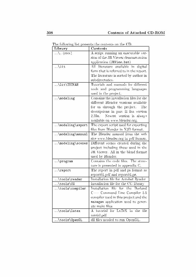
308 Contents of Atta hed CD-ROMThe following list presents the ontents on the CD.Library Contents..\. (root) A s ript running an exe utable ver-sion of the JR Viewer demonstrationappli ation (JRView.bat)..\lit All literature available in digitalform that is referred to in the report.The literature is sorted by author insubdire tories...\lit\TUTMAN Tutorials and manuals for di�erenttools and programming languagesused in the proje t...\modeling Contains the installation �les for thedi�erent Blender versions availablefor us through the proje t. Thedes riptions in part II �ts version2.33a. Newest version is alwaysavailable on www.blender.org...\modeling\export The export s ript used for exporting�les from Blender in X3D format...\modeling\manual The Blender manual from the website www.blender.org in pdf format...\modeling\s enes Di�erent s enes reated during theproje t in luding those used in theJR Viewer. All in the blend formatused by Blender...\program Contains the ode �les. The stru -ture is presented in appendix C...\report The report in pdf and ps format asreport01.pdf and report01.ps...\tools\reader Installation �le for A robat Reader..\tools\CG Installation �le for the CG library..\tools\ ompiler Installation �le for the BorlandC++ Command Line Compiler 5.5 ompiler used in this proje t and themakegen appli ation used to gener-ate make �les...\tools\latex A tutorial for LaTeX in the �letnssitl.pdf..\tools\OpenGL dll �les needed to run OpenGL.

Appendix BHistori al RemarksThe nature of light has been studied and investigated ever sin e man beganto philosophize.Presumably the Pythagoreans (�582�500 BC.) of an ient Gree e putforth the �parti le� theory of light [138℄ in whi h it is hypothesized that theeyes send rays to obje ts and that these rays give us information about theobje t's shape and olor [96℄.Though we know, today, that light is emitted from light sour es, notthe eyes, the mathemati al model des ribed by the an ient philosophers isbasi ally the same as when we tra e rays from the eyes in ba kward raytra ing.The �rst to theorize that the medium of sight (light) is from the obje tand is re eived by the visual per eption organ (eye) is Empedo les (�480BC.) [96℄. However, many years should pass before this theory was generallya epted.Eu lid's Opti s (�300 BC.) is the oldest surviving work on geometri alopti s (or ray opti s) [32℄. He notes that light travels in straight lines. Fur-thermore the prin iples of perspe tive are established and the law of re�e tionis given [33℄, presented below in its modern enun iation [116℄:The re�e ted ray lies in the plane of in iden e;the angle of re�e tion equals the angle of in iden e.Approximately one and a half enturies later Hero (or Heron) of Alexan-dria (�150 BC.) showed geometri ally that the a tual path taken by a rayof light re�e ted from a plane mirror is shorter than any other re�e ted paththat might be drawn between the sour e and the point of observation [4℄.The prin iple of the path of minimum distan e is later known as Hero's Prin- iple. This result leads towards Fermat's Prin iple that should later be omeone of the four fundamental postulates of ray opti s [116℄.Refra tion when light passes from air into water or glass was observedand studied by Cleomedes (50 AD.) and Ptolemy (130 AD.). In the work of

310 Histori al Remarksthe latter it is suggested that the angle of refra tion is proportional to theangle of in iden e [4℄. Later this shall result in Snell's law.Through logi and experimentation the Arabian s ientist and s holarIbn al-Haitham1 known to the Europeans as Alhazen (965�1039 AD.) �nallydis ounted the theory that vision issues forth from the eye. He used a fore-runner of the amera obs ura (a pinhole amera) as a model for the eye andinvestigated both spheri al and paraboli mirrors. He was aware of spheri alaberration and also investigated the magni� ation produ ed by lenses andatmospheri refra tion. His work in�uen ed all later investigations on light[138, 4, 82℄.Quite a few enturies should now pass before the next break throughin the theory of light would emerge. Opti s had again be ome an ex it-ing area of resear h with the invention of teles opes and mi ros opes in theearly seventeenth entury. In 1611 Johannes Kepler dis overed total inter-nal re�e tion and des ribed the small angle approximation to the law ofrefra tion [30℄. A de ade later, in 1621, Willebrord Snell dis overed the re-lationship between the angle of in iden e and the angle of refra tion whenlight passes from one transparent medium to another [4℄. This relationshipis alled Snell's law, whi h led to the law of refra tion. The same law was,in 1637, independently dis overed and formulated in terms of sines by RenéDes artes. It was published in his Dis ourse on Method ontaining a s ien-ti� treatise on opti s [26℄. In its modern form the law of refra tion is givenas [116℄:The refra ted ray lies in the plane of in iden e; the angle ofrefra tion �2 is related to the angle of in iden e �1 by Snell's law,n1 sin �1 = n2 sin �2Pierre de Fermat's Prin iple of �least time�, a ording to whi h a ray oflight follows the path whi h takes it to its destination in shortest time, isenun iated in 1657 [4℄. From this prin iple both the laws of re�e tion andrefra tion an be dedu ed. Today Fermat's Prin iple has a slightly di�erentpresentation [116℄:Opti al rays traveling between two points, A and B, follow a pathsu h that the time of travel (or the opti al path length) betweenthe two points is an extremum relative to neighboring paths.The extremum may be a minimum, a maximum, or a point of in�e tion.It is, however, usually a minimum, in whi h ase Fermat's original formula-tion is true. In a homogenous medium the index of refra tion (n) is the same1Full name: Abu Ali Mohamed ibn al-Hasan Ign al-Haytham.

311everywhere, and so is the speed of light. The path of minimum light is thenalso the path of minimum distan e, whi h leads to the following formulationof Hero's Prin iple: In a homogenous medium light travels in straight lines[116℄. De idedly Hero's Prin iple is a spe ial ase of Fermat's Prin iple.In 1665, Grimaldi and Hooke on lude upon their observations of di�ra -tion, the phenomenon where light �bends� around obstru ting obje ts, thatlight is a �uid that exhibits wave-like motion. Hooke proposed a wave theoryof light to explain this behavior [30℄. Around the same time Isaa Newtondes ribes his theory of olor using a prism to show that white light is a ombination of di�erent olors [4℄ (the phenomenon is alled dispersion).Ole Rømer dedu es an approximate value of the speed of light in 1676.This is done from detailed observations of the e lipses of the moons of Jupiter.From Rømer's data, a value of about 2 � 108m=s is obtainable [4℄.A major milestone for a wave theory of light is the "Traite de Lumiere"published by Huygens in 1690. He onsidered that light is transmittedthrough an all-pervading aether that is made up of small elasti parti les,ea h of whi h an a t as a se ondary wavelet [4℄. Huygens also dis overedthe phenomenon of polarization during his experiments [30℄. His theory was,though able to explain many of the known propagation hara teristi s oflight, put aside when Newton published his "Opti ks" (1704) in whi h heput forward the view that light is orpus ular (parti les traveling in straightlines).A entury should pass before Thomas Young (1801) provided the ne es-sary support for a wave theory of light by demonstration of the prin iple ofinterferen e through his double-slit experiment.In 1816, Augustin Jean Fresnel presents a rigorous treatment of di�ra -tion and interferen e phenomena showing that they an be explained in termsof a wave theory of light. Later (1821) he presented the laws whi h enablethe intensity and polarization of re�e ted and refra ted light to be al u-lated, [4, 30℄. Modern text books present the Fresnel equations as follows[60℄: �k = �2 os �1 � �1 os �2�2 os �1 + �1 os �2�? = �1 os �1 � �2 os �2�1 os �1 + �2 os �2Fr(�) = 12(�2k + �2?)Using the wave theory Helmholtz (1821�1894) re ords the urves for thebasi mixing olors: ultramarine blue, green, and red. These three olorsand their mixing olors are as ribed to three kinds of olor sensitive re ep-tors in the eye. This theory be omes known as the Young-Helmholtz ThreeComponent Theory [96℄.

312 Histori al RemarksMaxwell puts forth his famous theory of the ele tromagneti �eld in1865. Taking earlier experimental and theoreti al work of Coulomb, Poisson,Ørsted, Ampere, Faraday, and others; he ompleted the theory [76℄. Fromhis studies of the equations des ribing ele tri and magneti �elds, it wasfound that the speed of an ele tromagneti wave should, within experimen-tal error, be the same as the speed of light. Maxwell on luded that light isa form of ele tromagneti wave [4℄.Heinri h Hertz validated Maxwells theory experimentally [76℄ and in1887 he a identally dis overed the photoele tri e�e t, whi h is the pro esswhereby ele trons are liberated from materials under the a tion of radiantenergy [30℄. An e�e t that an not be des ribed by the wave model.Nevertheless light an, at this point, be des ribed as the visible part of thespe trum of ele tromagneti radiation. Ele tromagneti waves range fromradio waves, whi h an have wavelengths of kilometers, to osmi rays withwavelengths of less than 10�10 entimeter. The range of visible wavelengthsis approximately 0:4 � 0:7�m, and it is in luded in the area of ele tromag-neti waves dete ted as heat radiation [121℄. The resear h area of thermalradiation heat transfer is therefore of interest to the theory of light.In 1879 Joseph Stefan published an experimental investigation of thespe tral distribution of heat transfer from bodies of di�erent temperatures.His results were a number of urves showing that the emitted power in reaseswith in reasing temperature, and that the maximum point of a distributionis found at shorter wavelengths when the temperature in reases [11℄.A few years later (1884) Ludwig Boltzmann was able to dedu e theo-reti ally that the emissive power varies with the temperature power four.Similarly Willy Wien2 dedu ed the displa ement law a de ade later (1896):�maxT = onstantSin e heat and light is ele tromagneti waves, many attempts to �nd a onne tion between the experimental results of Stefan and the theoreti alresults of Boltzmann and Wien were ondu ted using Maxwell's equations.However, it was only possible to �nd fun tional expressions that ould on-�rm Stefan's experimental results at very long or at very short wavelengths[11℄. In 1901 Max Karl Ernst Ludwig Plan k provided the missing on- ept. He proposed the existen e of a light quantum, based on this quantumtheory he was able to explain the spe trum of radiation emitted from abla kbody [107℄. Plan k found it ne essary to introdu e a universal on-stant des ribed as the quantum of a tion, now known as Plan k's onstant(h � 6:63 � 10�34Js) [4℄.Plan k's theory remained mystifying until Albert Einstein in 1905 ex-plained the photoele tri e�e t on the basis that light is quantized, the2Willy was a onvenient ni kname sin e his full name was Wilhelm Carl Werner OttoFritz Franz Wien.

313quanta would subsequently be ome known as photons [4℄. During the nexttwo de ades s ientists re ast all of physi s to be onsistent with Plan k'stheory [82℄. However, the wave model of light was still ne essary to des ribephenomena su h as interferen e and di�ra tion - Niels Bohr alled this the omplementary nature of light [60℄.In 1913, Bohr put forth a theory explaining the observation that atomsabsorb and emit light at parti ular frequen ies that are hara teristi ofthe atom [4℄. His theory was based on quantum me hani s. By onsider-ing submi ros opi phenomena, resear hers su h as Bohr, Born, Heisenberg,S hrödinger, Pauli, De Broglie, Dira , and others, have been able to explainthe omplementary nature of light [30℄.To summarize four major models for the explanation of light have beenput forth through times. Those are ray opti s, wave opti s, ele tromagneti opti s, and quantum (or photon) opti s. Ea h model has a set of postulateson whi h all possible results of that model depend. The more advan edmodels in lude the simpler ones and therefore the postulates of ray opti sfor example follows naturally from the postulates of wave opti s. A thoroughexplanation is provided in [116℄.

314 Histori al Remarks

Appendix CStru ture of Sour e Files andLibraries

316 Stru ture of Sour e Files and LibrariesBMesh

CG

engine

file

headers

Components

AdjFace.cpp load_mesh.cpp OneRing.cpp TexmapDraw.cpp AdjFaceList.cpp Material.cpp OneRingDB.cpp TriMesh.cpp Bmesh.lib mesh_plane.cpp Parse.cpp vrml_save.cpp draw.cpp MeshFunc.cpp smooth.cpp x3d_load.cpp Edge.cpp obj_load.cpp TexCoord.cpp X3DBMesh.cpp Instance.cpp Object.cpp Texmap.cpp

direct.cg indirect.cg phongshade_fp.cg subsurf_fp.cg direct_fp.cg indirect_fp.cg position.cg translucent_fp.cg directVertOnly.cg indirSubSurf_fp.cg reflection.cg extrude.cg normal.cg refraction.cg

AreaLightSource.cpp PointLightSource.cpp LightSource.h Timer.h BSPTree.cpp Ray.cpp Material.h Triangle.h Camera.cpp Sphere.cpp Mesh.h Window.h envmap.cpp Traingle.cpp nnraytrace.h World.h Material.cpp World.cpp Object3D.h AABB.h Mesh.cpp AABB.cpp PhotonMap.h nnraytrace.cpp BSPTree.h Plane.h PhotonMap.cpp Camera.h Ray.h Plane.cpp envmap.h Sphere.h

file.cpp FinalScene.x3d file.h

AdjFace.h Material.h Parse.h AdjFaceList.h mesh_plane.h TexCoord.h draw.h Mesh4FaceModifier.h TexMap.h Edge.h MeshFunc.h TexmapDraw.h Instance.h obj_load.h TriMesh.h Light.h Object.h vrml_save.h load_mesh.h OneRing.h x3d_load.h loader.h OneRingDB.h X3DBMesh.h

Timer.h

BMesh

GL extgl.h glui.h glut.h

ME MEdouble2.h MEfloat3x3.h MESqMatrix.h MEdouble3.h MEfloat4.h MEVector.h MEdouble3x3.h MEfloat4x4.h Quaternion.h MEdouble4.h MEfloatQuat.h MEdouble4x4.h MEint2.h MEfloat2.h MEint3.h MEfloat3.h MEMatrix.h

expat.h Timer.h

logo bitmap.cpp bitmap.h logo.h logo.cpp JRLogo2.bmp

MEsrc MEfloat3.cpp MEfloat4.cpp MEint3.cpp

photonmaps photonmaps.cpp photonmaps.h

radiosity Hemicube.cpp SceneGraph.cpp Mesher.h Tools.h IdexedFaceSet.cpp SceneGraphLoader.cpp ProgRef.h Resource1.xml Loader.cpp SceneGrapTools,cpp radiosity.h Resource2.xml Mesher.cpp Tools.cpp ResourceLoader.h cornell_1.x3d ProgRef.cpp DataFormat.h SceneGraph.h cornell_2.x3d radiosity.cpp Hemicube.h SceneGraphLoader.h ResourceLoader.cpp Loader.h SceneGraphTools.h

317

raytracing

textures

TrackBall

JRLogo32.ico menu.rc menuFlags.h message.h main.cpp resource.h

rasterization rasterization.cpp rasterization.h

raytracing.cpp raytracing.h

textures.cpp textures.h

TrackBall.cpp TrackBall.h

318 Stru ture of Sour e Files and Libraries

Bibliography[1℄ Tomas Akanine-Möller and Ulf Assarsson. Approximate soft shadowson arbitrary surfa es using penumbra wedges. In Rendering Te hniques'02 (Pro . of the Thirteenth Eurographi s Workshop on Rendering),pages 297�306, 2002.[2℄ Tomas Akenine-Möller and Eri Haines. Real-Time Rendering. A KPeters, Nati k, Massa husetts, se ond edition, 2002.[3℄ Edward Angel. Intera tive Computer Graphi s: A Top-Down Approa hUsing OpenGLTM. Addison-Wesley, third edition, 2003.[4℄ A brief history of opti s. http://members.aol. om/WSRNet/D1/hist.htm. A - essed 3rd of June 2004.[5℄ James Arvo and David B. Kirk. Parti le transport and image synthe-sis. Computer Graphi s (SIGGRAPH '90 Pro eedings), 24(4):63�66,August 1990.[6℄ Ian Ashdown. Photometry and radiometry: A tour guide for omputergraphi s enthusiasts. www.helios32. om/Measuring Light.pdf, O tober 2002.[7℄ Ulf Assarsson. A Real-Time Soft Shadow Volume Algorithm. PhDthesis, Chalmers University of Te hnology, 2003.[8℄ Ulf Assarsson, Mi hael Dougherty, Mi hael Mounier, and TomasAkenine-Möller. An optimized soft shadow volume algorithmwith real-time performan e. In M Doggett, W. Heidri h,W. Mark, and A. S hilling, editors, Pro eedings of the ACM SIG-GRAPH/EUROGRAPHICS Conferen e on Graphi s Hardware, pages33�40. Eurographi s Asso iation, 2003.[9℄ James F. Blinn. Models of light re�e tions for omputer synthesizedpi tures. Computer Graphi s (SIGGRAPH '77 Pro eedings), pages192�198, July 1977.[10℄ James F. Blinn and Martin E. Newell. Texture and re�e tion in om-puter generated images. Communi ations of the ACM, 19(10):542�547,O tober 1976.

320 BIBLIOGRAPHY[11℄ Erik Both and Gunnar Christensen. Termodynamik. Den private In-geniørfond, third edition, 2002.[12℄ Chris Brennan. Shadow volume extrusion using a vertex shader. InWolfgang F. Engel, editor, ShaderX: Vertex and Pixel Shader Program-ming Tips and Tri ks. Wordware, May 2002.[13℄ Nathan A. Carr, Jesse D. Hall, and John C. Hart. GPU algorithms forradiosity and subsurfa e s attering. In Pro eedings of the ACM SIG-GRAPH/EUROGRAPHICS onferen e on Graphi s hardware, pages51�59. Eurographi s Asso iation, 2003.[14℄ Jens Mi hael Carstensen, editor. Image Analysis, Vision, and Com-puter Graphi s. IMM, Te hni al University of Denmark, Lyngby, 2001.[15℄ Subrahmanyan Chandrasekhar. Radiative Transfer. Dover Publi a-tions, In ., New York, 1960. Unabridged and slightly revised editionof the work �rst published in 1950.[16℄ Keshav Channa. Light mapping - theory and implementation.http://www.�ip ode. om/arti les/arti le_lightmapping.shtml, July 2003. A - essed 31st of August 2004.[17℄ Per H. Christensen. Adjoints and importan e in rendering: Anoverview. IEEE Transa tions on Visualization and Computer Graph-i s, 9(3), 2003.[18℄ Mi hael F. Cohen and Donald P. Greenberg. The hemi- ube: A ra-diosity solution for omplex environments. Computer Graphi s (SIG-GRAPH '85 Pro eedings), 19(3):31�40, July 1985.[19℄ Mi hael F. Cohen and John R. Walla e. Radiosity and Realisti ImageSynthesis. A ademi Press Professional, 1993.[20℄ Robert L. Cook, Thomas Porter, and Loren Carpenter. Distributed raytra ing. Computer Graphi s (SIGGRAPH '84 Pro eedings), 18(3):137�145, July 1984.[21℄ Robert L. Cook and Kenneth E. Torran e. A re�e tan e model for omputer graphi s. ACM Transa tions on Computer Graphi s, 1(1):7�24, 1982.[22℄ Franklin C. Crow. Shadow algorithms for omputer graphi s. Com-puter Graphi s (SIGGRAPH '77 Pro eedings), 11(3):242�248, July1977.[23℄ Haskell Brooks Curry and Robert Feys. Combinatory Logi , volume 1.North Holland Publishing Company, Amsterdam, 1958.

BIBLIOGRAPHY 321[24℄ Erik B. Dam, Martin Ko h, and Martin Lillholm. Quaternions, interpo-lation and animation. Te hni al Report DIKU-TR-98/5, Departmentof Computer S ien e, University of Copenhagen, July 1998.[25℄ Mark de Berg, Mar van Kreveld, Mark Overmars, and OtfriedS hwartzkopf. Computational Geometry: Algorithms and Appli ations.Springer, Berlin, se ond edition, 2000.[26℄ René Des artes. Dis ourse on Method, Opti s, Geometry, and Meteo-rology. Ha kett Publishing Co, In , revised edition, May 2001.[27℄ Kirill Dmitriev, Stefan Brabe , Karl Myszkowski, and Hans-Peter Sei-del. Intera tive global illumination using sele tive photon tra ing. InRendering Te hniques '02 (Pro . of the Thirteenth Eurographi s Work-shop on Rendering), pages 21�34, 2002.[28℄ Craig Donner and Henrik Wann Jensen. Faster gpu omputations usingadaptive re�nement. In Pro eedings of SIGGRAPH 2004, Te hni alSket hes, August 2004.[29℄ Julie Dorsey, Alan Edelman, Henrik Wann Jensen, Justin Legakis, andHans Køhling Pedersen. Modeling and rendering of weathered stone.In Pro eedings of SIGGRAPH 1999, pages 411�420, 1999.[30℄ Philip Dutré, Philippe Bekaert, and Kavita Bala. Advan ed GlobalIllumination. A K Peters, Nati k, Massa husetts, 2003.[31℄ Jens Eising. Lineær algebra. Institut for Matematik, DanmarksTekniske Universitet, 1997.[32℄ Adventures in ybersound: Eu lid. http://www.a mi.net.au/AIC/EU-CLID_BIO.html. A essed 14th of May 2004.[33℄ Eu lid. Opti s. http://www. alstatela.edu/fa ulty/hmendel/An ient Mathe-mati s/Eu lid/Opti s/Opti s.html. A essed 14th of May 2004.[34℄ Cass Everitt and Mark J. Kilgard. Pra ti al and robust sten iledshadow volumes for hardware-a elerated rendering. NVIDIA WhitePaper, Mar h 2002. http://developer.nvidia. om.[35℄ Kasper Fauerby and Carsten Kjær. Real-time soft shadows in a gameengine. Master's thesis, Department of Computer S ien e, Universityof Aarhus, De ember 2003.[36℄ Randima Fernando and Mark J. Kilgard. The Cg Tutorial: The De�ni-tive Guide to Programmable Real-Time Graphi s. Addison-Wesley,2003.

322 BIBLIOGRAPHY[37℄ F. Fisher and A. Woo. R.e versus n.h spe ular highlights. In Paul S.He kbert, editor, Graphi s Gems IV, pages 388�400. A ademi Press,1994.[38℄ Foley, van Dam, Feiner, and Hughes. Computer Graphi s: Prin i-ple and Pra ti e. The Systems Programming Series. Addison-Wesley,se ond edition, 1997.[39℄ Aa. Frøslev-Nielsen. Lys, farver og farvers reproduktion. Te hni alreport, Den Gra�ske Højskole, 1996.[40℄ Cindy M. Goral, Kenneth E. Torran e, Donald P. Greenberg, and Ben-nett Battaile. Modeling the intera tion of light between di�use sur-fa es. Computer Graphi s (SIGGRAPH '84 Pro eedings), 18(3):213�222, July 1984.[41℄ Henri Gouraud. Computer display of urved surfa es. Te hni al ReportUTEC-CS -71-113, Department of Computer S ien e, Uni ersity ofUtah, June 1971. Also in IEEE Transa tions on Computers, vol. C-20,pp. 623�629, June 1971.[42℄ Jens Gravesen. Di�erential Geometry and Design of Shape and Mo-tion. Department of Mathemati s, Te hni al University of Denmark,November 2002. Le ture notes for 01243.[43℄ Gene Greger, Peter Shirley, Philip M. Hubbard, and Donald P. Green-berg. The irradian e volume. IEEE Computer Graphi s & Appli a-tions, 18(2):32�43, 1998.[44℄ Johannes Günther, Ingo Wald, and Philipp Slusallek. Realtime austi susing distributed photon mapping. In H. W. Jensen and A. Keller,editors, Eurograhi s Symposium on Rendering, 2004.[45℄ Pat Hanrahan and Wolfgang Krueger. Re�e tion from layered surfa esdue to subsurfa e s attering. Computer Graphi s (Pro . SIGGRAPH'93), pages 165�174, August 1993.[46℄ Xuejun Hao, Thomas Baby, and Amitabh Varshney. Intera tive sub-surfa e s attering for translu ent meshes. In Pro eedings 2003 ACMSymposium on Intera tive 3D Graphi s, April 2003.[47℄ Kevin Hawkins and Dave Astle. OpenGL Game Programming. PrimaTe h's Game Development Series. Premier Press, 2001.[48℄ Paul S. He kbert. Adaptive radiosity textures for bidire tional raytra ing. Computer Graphi s (SIGGRAPH '90 Pro eedings), 24(4):145�154, August 1990.

BIBLIOGRAPHY 323[49℄ Tim Heidmann. Real shadows real time. IRIS Universe, (18):28�31,1991.[50℄ Heinri h Hey. Photorealisti and Hardware A elerated Rendering ofComplex S enes. Ph.D. dissertation, Te hnis hen Universität Wien,Te hnis h-Naturwissens haftli he Fakultät, May 2002.[51℄ Bjarke Jakobsen, Niels J. Christensen, Bent D. Larsen, and Kim S. Pe-tersen. Boundary orre t real-time soft shadows. In Computer Graphi sInternational 2004 Pro eedings, pages 232�239, June 2004.[52℄ Greg James and Simon Green. Real-time animated translu en y.Game Developers Conferen e, 2004. http://developer.nvidia. om/obje t/gd _2004_presentations.html.[53℄ Henrik Wann Jensen. Global illumination via bidirektional monte arloray tra ing. Master's thesis, Te hni al University of Denmark, 1993.[54℄ Henrik Wann Jensen. Importan e driven path tra ing using the photonmap. In P. Hanrahan and W. Purgathofer, editors, Rendering Te h-niques '95 (Pro . of the Sixth Eurographi s Workshop on Rendering),pages 326�335. Vienna: Springer-Verlag, June 1995.[55℄ Henrik Wann Jensen. Global illumination using photon maps. InXavier Pueyo and Peter S hröder, editors, Rendering Te hniques '96(Pro . of the Seventh Eurographi s Workshop on Rendering), pages21�30. Vienna: Springer-Verlag, 1996.[56℄ Henrik Wann Jensen. The Photon Map in Global Illumination. PhDthesis, Te hni al University of Denmark, September 1996.[57℄ Henrik Wann Jensen. Rendering austi s on non-lambertian surfa es.In Wayne A. Davis and Ri hard Bartels, editors, Graphi s Interfa e'96, pages 116�121, Toronto, May 1996. Canadian Information Pro- essing So iety, Canadian Human-Computer Communi ations So iety.[58℄ Henrik Wann Jensen. Parallel global illumination using photon map-ping. SIGGRAPH 2000 Course Notes, New York: ACM Press, July2000.[59℄ Henrik Wann Jensen. A pra ti al guide to global illumination usingphoton maps. SIGGRAPH 2000 Course Notes, New York: ACM Press,July 2000.[60℄ Henrik Wann Jensen. Realisti Image Synthesis Using Photon Map-ping. A K Peters, Nati k, Massa husetts, 2001.

324 BIBLIOGRAPHY[61℄ Henrik Wann Jensen and Juan Buhler. A rapid hierar hi al renderingte hnique for translu ent materials. In J. F. Hughes, editor, Pro eed-ings of SIGGRAPH 2002, pages 576�581, July 2002.[62℄ Henrik Wann Jensen and Niels Jørgen Christensen. E� iently ren-dering shadows using the photon map. In Harold P. Santo, editor,Compugraphi s '95, pages 285�291, De ember 1995.[63℄ Henrik Wann Jensen and Niels Jørgen Christensen. Photon maps inbidire tional monte arlo ray tra ing of omplex obje ts. Computers& Graphi s, 19(2):215�224, Mar h 1995.[64℄ Henrik Wann Jensen, Justin Legakis, and Julie Dorsey. Rendering ofwet materials. In D. Lis hinski and G. W. Larsoi, editors, RenderingTe hniques '99 (Pro . of the Tenth Eurographi s Workshop on Render-ing), pages 273�282. Vienna: Springer-Verlag, 1999.[65℄ Henrik Wann Jensen, Stephen R. Mars hner, Mar Levoy, and PatHanrahan. A pra ti al model for subsurfa e light transport. In Pro- eedings of SIGGRAPH 2001, pages 511�518, August 2001.[66℄ James T. Kajiya. The rendering equation. Computer Graphi s (SIG-GRAPH '86 Pro eedings), 20(4):143�150, August 1986.[67℄ Ashraf A. Kassim and B. V. K. Vijaya Kumar. The wave expansionneural network. Neuro omputing, 16:237�258, 1997.[68℄ Ashraf A. Kassim and B. V. K. Vijaya Kumar. Path planners basedon the wave expansion neural network. Roboti s and Autonomous Sys-tems, 26:1�22, 1999.[69℄ A. Keller. Instant radiosity. In Turner Whitted, editor, Pro eedings ofSIGGRAPH 1997, pages 49�56, Reading, 1997. MA: Addison-Wesley.[70℄ Mark J. Kilgard. Improving shadows and re�e tions viathe sten il bu�er. NVIDIA White Paper, November 1999.http://developer.nvidia. om.[71℄ Mi hail G. Lagoudakis. Hop�eld neural network for dynami path plan-ning and obsta le avoidan e. Semester proje t for CMPS 588 �NeuralNetworks�, 1997. http://www. s.duke.edu/�mgl/a adpape.html.[72℄ Bent Dalgaard Larsen. Global Illumination for Real-Time Appli ationsby Simulating Photon Mapping. PhD thesis, Informati s and Mathe-mati al Modeling, Te hni al University of Denmark, 2004.[73℄ Bent Dalgaard Larsen and Niels Jørgen Christensen. Optimizing pho-ton mapping using multiple photon maps for irradian e estimates. InWSCG'2003 Posters Pro eedings, pages 77�80, February 2003.

BIBLIOGRAPHY 325[74℄ Bent Dalgaard Larsen and Niels Jørgen Christensen. Simulating pho-ton mapping for real-time appli ations. In H. W. Jensen and A. Keller,editors, Eurographi s Symposium on Rendering, 2004.[75℄ Hendrik P. A. Lens h, Mi hael Goesele, Philippe Bekaert, and JanKautz. Intera tive rendering of translu ent obje ts. In Pro . IEEEPa i� Graphi s 2002, pages 214�224, 2002.[76℄ Mal olm Longair. Light and olour. In Lamb and Bourriau, editors,Colour: Art and S ien e. Cambridge University Press, 1997.[77℄ Rafal Mantiuk, Sumanta Pattanaik, and Karol Myszkowski. Cube-map data stru ture for intera tive global illumination omputation indynami di�use environments. In Pro eedings of International Con-feren e on Computer Vision and Graphi s, pages 530�538, September2002.[78℄ Morgan M Guire, John F. Hughes, Kevin T. Egan, Mark J. Kilgard,and Cass Everitt. Fast, pra ti al and robust shadows. NVIDIA WhitePaper, November 2002. http://developer.nvidia. om.[79℄ Tom M Reynolds, David Blythe, Brad Grantham, Mark J. Kilgard,and S ott Nelson. Advan ed graphi s programming te hniques usingopengl. SIGGRAPH 1999 Course Notes, July 1999.[80℄ Tom Mertens, Jan Kautz, Philippe Bekaert, Frank Van Reeth, andHans-Peter Seidel. E� ient rendering of lo al subsurfa e s attering.In Jon Rokne, Reinhard Klein, and Wenping Wang, editors, 11th Pa- i� Conferen e on Computer Graphi s and Appli ations, pages 51�58,Canmore, Canada, O tober 2003. IEEE.[81℄ Tom Mertens, Jan Kautz, Philippe Bekaert, Hans-Peter Seidel, andFrank Van Reeth. Intera tive rendering of translu ent deformable ob-je ts. In Per Christensen and Daniel Cohen-Or, editors, Eurographi sSymposium on Rendering, pages 130�140, June 2003.[82℄ Light: History of light theories. Mi rosoft r En arta r Online En y- lopedia, 2004. Reviewed by John H. Marburger. http://en arta.msn. om.A essed 3rd of June 2004.[83℄ Brook Miles. theForger's Win32 API Tutorial, 1998�2003. Version 2.0.http://winprog.org/tutorial/.[84℄ Tren hard More, Jr. Notes on the development of a theory of ar-rays. Te hni al Report 320-3016, IBM S ienti� Ctr., Philadelphia,Pa., 1973.

326 BIBLIOGRAPHY[85℄ Tren hard More, Jr. Notes on the axioms for a theory of arrays. Te h-ni al Report 320-3017, IBM S ienti� Ctr., Philadelphia, Pa., 1973.[86℄ Tren hard More, Jr. Axioms and theorems for a theory of arrays. IBMJournal of Resear h and Development, 17(2):135�175, 1973.[87℄ L. Neumann, M. Feda, M. Kopp, andW. Purgathofer. A new sto hasti radiosity method for highly omplex s enes. In Rendering Te hniques'94 (Pro . of Fifth Eurographi s Workshop on Rendering), pages 195�206, Darmstadt, Germany, June 1994.[88℄ F. E. Ni odemus, J. C. Ri hmond, J. J. Hsia, I. W. Ginsberg, andT. Limperis. Geometri al onsiderations and nomen lature for re-�e tan e. Te hni al report, National Bureau of Standards (US), O to-ber 1977.[89℄ Fred E. Ni odemus, editor. Self-Study Manual on Opti al Radia-tion Measurements. National Institute of Standards and Te hnol-ogy, U.S. Department of Commer e, 1976�1985. NBS Te hni alnotes, Series 910-1 through 8. Chapters were published as ompleted.http://physi s.nist.gov/Divisions/Div844/manual/studymanual.html.[90℄ Kasper Høy Nielsen. Real-time hardware-based photorealisti render-ing. Master's thesis, Informati s and Mathemati al Modeling, Te hni- al University of Denmark, November 2000.[91℄ Kasper Høy Nielsen and Niels Jørgen Christensen. Real-time re ur-sive spe ular re�e tions on planar and urved surfa es using graphi shardware. Journal of WSCG, 3:91�98, 2002.[92℄ Mangesh Nijasure. Intera tive global illumination on the graphi s pro- essing unit. Master's thesis, B. E. University of Bombay, November2003.[93℄ Mangesh Nijasure, Sumanta Pattanaik, and Vineet Goel. Intera tiveglobal illumination in dynami environments using ommodity graph-i s hardware. In Pro eedings of the 11th Pa i� Conferen e on Com-puter Graphi s and Appli ations, pages 450�454, 2003.[94℄ T. Nishita and E. Nakamae. Continuous tone representation of 3-d obje ts taking a ount of shadows and interre�e tion. ComputerGraphi s (SIGGRAPH '85 Pro eedings), 19(3):23�30, July 1985.[95℄ Cornell University Program of Computer Graphi s. Cornell box data.http://www.graphi s. ornell.edu/online/box/data.html, April 1998. A essed25th of August 2004.

BIBLIOGRAPHY 327[96℄ History of olor s ien e and theory. http://www.total.net/�daxx/ olour_theory_history.shtml. A essed 3rd of June 2004.[97℄ James M. Palmer. Radiometry and photometry faq. http://www.opti s.arizona.edu/Palmer/rpfaq/rpfaq.htm, O tober 2003.[98℄ Sybil P. Parker, editor. M Graw-Hill Di tionary of Mathemati s.M Graw-Hill, 1997.[99℄ S. N. Pattanaik and S. P. Mudur. The potential equation and im-portan e in illumination omputations. Computer Graphi s Forum,12(2):131�136, 1993.[100℄ Mark Pauly, Thomas Kollig, and Alexander Keller. Metropolis lighttransport for parti ipating media. In B. Pero he and H. Rushmeier,editors, Rendering Te hniques '00 (Pro . of the Eleventh Eurographi sWorkshop on Rendering), pages 11�22, New York, 2000. Springer.[101℄ Allan Pedersen. An introdu tion to array theory and nial. Ele -tri Power Engineering Department, Te hni al University of Denmark,September 1990.[102℄ Allan Pedersen and Jens Ulrik Hansen. Q'nial stand-by. Ele tri PowerEngineering Department, Te hni al University of Denmark, May 1988.[103℄ Ingmar Peter and Georg Pietrek. Importan e driven onstru tion ofphoton maps. In G. Drettakis and N. Max, editors, Rendering Te h-niques '98 (Pro . of the Ninth Eurographi s Workshop on Rendering),pages 269�280, Vienna: Springer-Verlag, 1998.[104℄ Joseph D. Petru elli, Balgobin Nandram, and Minghui Chen. AppliedStatisti s for Engineers and S ientists. Prenti e Hall, Upper SaddleRiver, New Jersey, 1999.[105℄ Matt Pharr and Pat Hanrahan. Monte arlo evaluation of non-linears attering equations for subsurfa e re�e tion. In Pro eedings of SIG-GRAPH 2000, pages 75�84, July 2000.[106℄ Bui Tuong Phong. Illumination for omputer-generated pi tures. Com-muni ations of the ACM, 18(6):311�317, June 1975.[107℄ Max Plan k. On the low of distribution of energy in the normal spe -trum. Ann. Physik, 4(3):553�563, 1901. http://dbhs.wvusd.k12. a.us/webdo s/Chem-History/Plan k-1901/Plan k-1901.html.[108℄ Timothy J. Pur ell, Craig Donner, Mike Cammarano, Henrik WannJensen, and Pat Hanrahan. Photon mapping on programmable graph-i s hardware. In M Doggett, W. Heidri h, W. Mark, and A. S hilling,

328 BIBLIOGRAPHYeditors, Pro eedings of the ACM SIGGRAPH/EUROGRAPHICS Con-feren e on Graphi s Hardware, pages 41�50. Eurographi s Asso iation,2003.[109℄ Brian Ramage. Fast radiosity using pixel shaders. Game Developer,11(7):20�39, August 2004.[110℄ Ravi Ramamoorthi and Pat Hanrahan. An e� ient representation forirradian e environment maps. In Pro eedings of SIGGRAPH 2001,pages 497�500, 2001.[111℄ Ravi Ramamoorthi and Pat Hanrahan. Frequen y spa e environmentmap rendering. In Pro eedings of SIGGRAPH 2002, pages 517�526,2002.[112℄ Barnett Ri h. Review of Elementary Mathemati s. S haum's Outlines,se ond edition, 1997. revised by Philip A. S hmidt.[113℄ Ton Roosendaal and Carsten Wartmann, editors. The O� ial BlenderGamekit: Intera tive 3-D for Artists. No Star h Press, San Fran is o,2003.[114℄ Holly E. Rushmeier. Extending the radiosity method to transmittingand spe ularly re�e ting surfa es. Master's thesis, Program of Com-puter Graphi s, Cornell University, 1986.[115℄ Holly E. Rushmeier and Kenneth E. Torran e. Extending the radios-ity method to in lude spe ularly re�e ting and translu ent materials.ACM Transa tions on Graphi s, 9(1):1�27, January 1990.[116℄ Bahaa E. A. Saleh and Malvin Carl Tei h. Fundamentals of Photoni s.John Wiley & Sons, New York, 1991.[117℄ Gernot S hau�er, Julie Dorsey, Xavier De oret, and François Sillion.Conservative volumetri visibility with o luder fusion. In Pro eedingsof SIGGRAPH 2000, pages 229�238, July 2000.[118℄ Christophe S hli k. An inexpensive BRDF model for physi ally basedrendering. Computer Graphi s Forum (Pro . of Eurographi s '94),13(3):233�246, September 1994.[119℄ Mark Q. Shaw. Evaluating the 1931 ie olor mat hing fun tions. Mas-ter's thesis, Center of Imaging S ien e, Ro hester Institute of Te hnol-ogy, Ro hester, New York, June 1999.[120℄ Ken Shoemake. Animating rotation with quaternion urves. ComputerGraphi s (SIGGRAPH '85 Pro eedings), pages 245�254, July 1985.

BIBLIOGRAPHY 329[121℄ Robert Siegel and John R. Howell. Thermal Radiation Heat Transfer.Taylor & Fran is, New York, fourth edition, 2002.[122℄ François X. Sillion, James R. Arvo, Stephen H. Westin, and Donald P.Greenberg. A global illumination solution for general re�e tan e distri-butions. Computer Graphi s (SIGGRAPH '91 Pro eedings), 25(4):187�196, August 1991.[123℄ Peter-Pike Sloan, Jan Kautz, and John Snyder. Pre omputed radian etransfer for real-time rendering in dynami , low-frequen y lighting en-vironments. ACM Transa tions on Graphi s, 21(3):527�536, July 2002.[124℄ Philipp Slussalek. Vision: An Ar hite ture for Physi ally-Based Ren-dering. Ph.D. dissertation, Der Teknis hen Fakultät der UniversitätErlangen-Nürnberg, 1995.[125℄ Bjarne Stroustrup. The C++ Programming Language. Addison-Wesley, Reading, Massa husetts, third edition, 1997.[126℄ Frank Suykens De Laet. On Robust Monte Carlo Algorithms for Multi-Pass Global Illumination. Ph.D. dissertation, Katholieke UniversiteitLeuven, Dept. of Computer S ien e, September 2002.[127℄ Greg Turk. Re-tiling polygonal surfa es. Computer Graphi s (SIG-GRAPH '92 Pro eedings), 26:55�64, July 1992.[128℄ Urb. lat. 1329 fol. 1 re to math04 NS.19.[129℄ Tom Vykruta. Simple and e� ient line-of-sight for 3d lands apes. InSteve Rabin, editor, AI Game Programming Wisdom. Charles RiverMedia, In ., Hingham, Massa husetts, 2002.[130℄ Mi hael Wand and Wolfgang Straÿer. Real-time austi s. In P. Brunetand D. Fellner, editors, Computer Graphi s Forum, volume 22(3),September 2003.[131℄ Lifeng Wang, Xi Wang, Xin Tong, Stephen Lin, Shimin Hu, BainingGuo, and Heung-Yeung Shum. View-dependent displa ement mapping.ACM Transa tions on Graphi s, 22(3):334�339, July 2003.[132℄ Gregory J. Ward. Measuring and modeling anisotropi re�e tion. Com-puter Graphi s (SIGGRAPH '92 Pro eedings), 26(2):265�272, July1992.[133℄ Gregory J. Ward, Fran is M. Rubinstein, and Robert D. Clear. A raytra ing solution for di�use interre�e tion. Computer Graphi s (SIG-GRAPH '88 Pro eedings), 22(4):85�92, August 1988.

330 BIBLIOGRAPHY[134℄ Alan Watt and Fabio Poli arpo. 3D Games: Real-Time Renderingand Software Te hnology, volume One of ACM SIGGRAPH Series.Addison-Wesley, 2001.[135℄ Alan Watt and Mark Watt. Advan ed Animation and Rendering Te h-niques: Theory and Pra ti e. Addison-Wesley, 1992.[136℄ Gerhard Weiss, editor. Multiagent Systems: A Modern Approa h toDistributed Arti� ial Intelligen e. The MIT Press, Cambridge, Mas-sa husetts, 1999.[137℄ Turner Whitted. An improved illumination model for shaded display.Communi ations of the ACM, 23(6):343�349, June 1980.[138℄ Bill Williams. A history of light and lighting. http://www.mts.net/�william5/history/hol.htm, 1999. Edition 2.2. A essed 3rd of June 2004.[139℄ Lan e Williams. Casting urved shadows on urved surfa es. ComputerGraphi s (SIGGRAPH '78 Pro eedings), pages 270�274, August 1978.[140℄ Lan e Williams. Pyramidal parametri s. Computer Graphi s (SIG-GRAPH '83 Pro eedings), 17(3):1�11, July 1983.[141℄ Tien-Tsin Wong, Wai-Shing Luk, and Pheng-Ann Heng. Sampling withhammersley and halton points. Journal of Graphi s Tools, 2(2):9�24,1997.[142℄ Chris Wynn and Sim Dietri h. Cube maps. NVIDIA Presentation,Mar h 2001. http://developer.nvidia. om.[143℄ Information te hnology | omputer graphi s and image pro essing |extensible 3d (x3d). ISO/IEC FDIS 19775:200x.[144℄ Information te hnology | omputer graphi s and image pro essing |extensible 3d (x3d) en odings. ISO/IEC 19776:200x.