1

Student

student@u.rochester.edu

CSC 290E

ODE Project

9 December 2010

Abstract

Systems in nature often depend on many variables that change with time, so modeling the behavior of these systems can sometimes by a complex affair. In order to model these systems, we use differential equations, which “express how related phenomena (variables) changing over time affect each other” (Brown). The main objective of the ODE project was to use MATLAB to numerically analyze differential equations. Results were gathered using both student-written derivative functions and MATLAB’s built-in ODE solving functions. The two main problems addressed were related to ballistics and environmental engineering.

Introduction Differential equations can be used to model the behavior of systems in nature. Some

applications include physics (F=ma, where a=𝑑𝑣

𝑑𝑡), electrical circuits, environmental engineering,

population dynamics, and many other fields. For this project, I focused on solving differential equations using MATLAB, not on deriving new laws or solving equations analytically. Deriving new laws can take years of study, and fun analytical methods of solving DEs can be learned in courses such as MTH 165. I specifically solved systems of ordinary differential equations (ODEs), which don’t use partial derivatives. One way to address a differential equation is by using matrices. Take, for example, the 2nd order

DE: 𝑦 ′′ + 𝑟 𝑥 𝑦 ′ + 𝑠 𝑥 = 𝑡(𝑥) We can rewrite this DE as a system of DEs:

𝑑

𝑑𝑥 𝑦𝑦′ =

0 1−𝑠(𝑥) −𝑟(𝑥)

𝑦𝑦′ +

0𝑡(𝑥)

We can then use some sort of program to plug in values and generate vectors of results.

Another approach is numerical integration. Because a derivative, 𝑑𝑦

𝑑𝑡, tells us how y changes with

t, we can linearly approximate y using a small change in t (we will call Δt). We also need an initial condition, y(0). Our estimation therefore becomes: y(Δt) = y(0) + y’(Δt). A familiar name for this process of numerical integration is “Euler’s method.” MATLAB has a powerful numerical integration tool, where the user needs to only supply a derivative function, a range of times, and an initial condition. MATLAB generates a vector of values that can be plotted to illustrate a solution to a DE.

2

Ballistics In the ODE project I worked through two separate projects, each with multiple sub-problems. The first major project was a ballistics problem based around the battle of Crecy. I wrote a derivative function to calculate x’, y’, x’’ and y’’. The differential equations were as follows: x’ = u y’ = v

x'' = - (1/(2m)) (ρ c a (u2 + v2) u/ 𝑢2 + 𝑣2))

y'' = -g - (1/(2m)) (ρ c a (u2 + v2) v/ 𝑢2 + 𝑣2)) I used the following base specifications: muzzle velocity = 150 m/s mass of cannonball = 5kg, air density ρ = 1.23, force of gravity g = 9.81, drag coefficient c = .5 diameter d =.1067 m area a = 𝜋𝑑2/4 I then used MATLAB’s built in ODE solver ode23 to solve the ODEs. Additionally, I wrote a script to return the distance travelled by the projectile using the last positive y value in the answer vector.

Part 1: Some Experimentation I first experimented by changing the values of constants such as launch angle and drag.

1. Launch Angle: a. We should see height increase as the launch angle approaches π/2 b. Horizontal range should (as predicted by behavior in a vacuum) reach a maximum at

some angle of launch close to to π/4

Figure 1 Figure 1 illustrates how launch angle affects trajectory. The green trajectory shows a launch angle of π/6, the blue trajectory shows a launch angle of π/4, and the pink trajectory shows a launch angle of π/3. The green ball travelled 1179.6 m, the blue

0 200 400 600 800 1000 1200 1400-100

0

100

200

300

400

500

600Cannonball Trajectory

Distance (m)

Hei

ght (

m)

3

ball travelled 1230.8 m and the pink ball travelled 1028.7 m. Figure 1 confirms the prediction that increasing launch angle will increase height. Figure 1 also suggests that maximum range is indeed achieved at a launch angle near π/4, but we do not know that angle yet.

2. Drag a. We expect rougher surfaces to decrease in speed faster (greater magnitude of x’’ and

y’’), therefore travelling shorter distances than smooth objects.

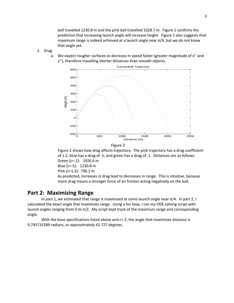
Figure 2 Figure 2 shows how drag affects trajectory. The pink trajectory has a drag coefficient of 1.2, blue has a drag of .5, and green has a drag of .1. Distances are as follows: Green (c=.1): 1926.6 m Blue (c=.5): 1230.8 m Pink (c=1.2): 796.2 m As predicted, increases in drag lead to decreases in range. This is intuitive, because more drag means a stronger force of air friction acting negatively on the ball.

Part 2: Maximizing Range In part 1, we estimated that range is maximized at some launch angle near π/4. In part 2, I calculated the exact angle that maximizes range. Using a for loop, I ran my ODE solving script with launch angles ranging from 0 to π/2. My script kept track of the maximum range and corresponding angle. With the base specifications listed above and c=.2, the angle that maximizes distance is 0.745731589 radians, or approximately 42.727 degrees.

0 500 1000 1500 2000 2500-200

-100

0

100

200

300

400

500

600Cannonball Trajectory

Distance (m)

Hei

ght (

m)

4

figure 3 Maximum projectile range = 1679.83 m. In a vacuum, maximum distance is achieved when the launch angle is π/4. Figure 3 shows that we must sacrifice some height to achieve maximum range due to factors such as air friction.

Part 3: Unorthodox Warfare In this part of the assignment I explored the trajectories of a non-traditional projectile, the meatball. I used a 6’’ (15.24 cm) diameter meatball with a drag coefficient of 0.7. I imagine that a 1 lb club pack of ground beef from Wegmans could be rounded into a ball with a diameter of roughly 6’’. To be safe, I estimated the weight of the meatball to be 1.5 pounds. Thus, mass is 0.68 kg. Using my optimization method described in part 2, I found the maximum range of my meatball to be 253.5 m with an elevation of .4284 radians (24.55°) and muzzle velocity of 300 m/s.

Figure 4 From figure 4 it may seem that a ball of meat could be a viable option if ammunition runs low. However, we have not yet taken into consideration the effect of wind on the projectile (we will address

0 200 400 600 800 1000 1200 1400 1600 1800 20000

50

100

150

200

250

300

350

400

450

500Cannonball Trajectory

Distance (m)

Hei

ght

(m)

0 50 100 150 200 2500

10

20

30

40

50

60

70

80

90

100Meatball Trajectory

Distance (m)

Hei

ght

(m)

5

wind in part 5). We will soon see that light-weight meatballs are affected greatly by wind, and blow off target quite easily.

Part 4: Variations in Air Density

Prior to this point in the project, we have assumed that air density is a constant value, ρ. Our base specifications set ρ to 1.23. However, actual air density varies with height. According to Wikipedia, air density can be expressed as:

where

and

sea level standard atmospheric pressure p0 = 101325 Pa

sea level standard temperature T0 = 288.15 K

Earth-surface gravitational acceleration g = 9.80665 m/s2.

temperature lapse rate L = 0.0065 K/m

universal gas constant R = 8.31447 J/(mol·K)

molar mass of dry air M = 0.0289644 kg/mo h = height in meters

I rewrote my derivative equations, using these equations to express air density as a function of height instead of as a constant.

Using the base specifications, a new cannonball trajectory looks like this (elevation of π/4):

Figure 5

0 200 400 600 800 1000 1200 1400-200

-100

0

100

200

300

400Cannonball Trajectory

Distance (m)

Heig

ht

(m)

6

Now compared to constant air density:

Figure 6 We can see from figure 6 that assuming constant air density slightly decreases range (the blue line is the trajectory assuming ρ=1.23). Under base specifications and elevation of π/4, the difference in range is approximately 13.8 m. Range (ρ=1.23): 1230.81 m Range (ρ changes with h): 1244.65 m I also compared maximum range using a muzzle velocity of 300 m/s and drag coefficient of .2:

0 200 400 600 800 1000 1200 1400-200

-100

0

100

200

300

400Cannonball Trajectory

Distance (m)

Hei

ght

(m)

0 500 1000 1500 2000 2500 3000 3500 40000

500

1000

1500Cannonball Trajectory

Distance (m)

Heig

ht

(m)

7

Figure 7 Figure 7 Shows the differences in trajectories between DEs with ρ=1.23 (blue) and with ρ varying with height (pink). Max range (pink): 4165.6 m at 40° Max range (blue): 4030.16 m at 39.1° It seems intuitive that the cannonball will travel further when air density varies with height. Air density decreases as height increases, so the magnitudes of x’’ and y’’ when air density varies will be smaller in comparison to x’’ and y’’ when density is constant. A smaller magnitude of x’’ and y’’ means less resistance and more range.

Part 5: Wind Now we must account for a west-east wind blowing. In order to model the affect of the wind on the cannonball, I edited my derivative functions and added z’ and z’’. z’’ looks similar to x’’, but instead of using u and v we use the velocity of the wind relative to the cannonball. My new equations looked like this: z’ = k z’’ = -(1/(2*m))*(rho*c*a*(wvel-k)2) , where wvel is wind velocity. I considered a wind of 100 mph, or 44.704 m/s. Under base specifications and at the launch angle that maximizes range, the trajectory as seen from above appears as follows:

Figure 8 Figure 8 shows the wind’s effect on the trajectory of the cannonball, blowing it approximately 120 m off target. The cannonball’s path looks parabolic because it is being accelerated. Do you remember our meatball projectile? When we account for wind, trajectory as seen from above looks like this:

0 200 400 600 800 1000 1200 14000

20

40

60

80

100

120

140Effect of Wind

distance in x direction

dis

tance in z

direction

8

Figure 9 Figure 9 shows that a meatball will be blown almost 180 m off-target during the course of its 253 m flight. It seems, therefore, that it would not serve well as a long range projectile, but perhaps could still splatter some goop on enemy helmets.

Environmental Engineering The second project in my ODE assignment dealt with environmental engineering. I obtained the individual problems from the reading, Environmental Engineering Science, by William W Nazaroff and Lisa Alvarez-Cohen Predominantly, this section involved modeling reaction rates using differential equations and MATLAB DE solvers. We can denote a kinetic chemical equation as follows:

𝑎𝐴 + 𝑏𝐵 ↔ 𝑐𝐶 + 𝑑𝐷 Where a, b, c, and d represent stoichiometric coefficients and A, B, C and D represent chemical species. The Reaction rate, R1, tells us the number of occurrences of the above reaction per unit time. Often, R1 is expressed in units of concentration per time. R1 therefore describes the rates at which concentration of chemical species increase and decrease. For the above reaction,

𝑅1 = − 1

𝑎 𝑑 𝐴

𝑑𝑡 = −

1

𝑏 𝑑 𝐵

𝑑𝑡 =

1

𝑐 𝑑 𝐶

𝑑𝑡 =

1

𝑑 𝑑 𝐷

𝑑𝑡

In order to express the overall rate law of the reaction, we need to only consider the concentration of the reactants in the reaction (in most cases). An example of a rate law is:

𝑅𝑦 = 𝑘𝑦 𝐴 𝛼 𝐵 𝛽

where ky is the rate constant, and α and β are empirical coefficients (Nazaroff, Alvarez-Cohen). The sum of α + β tells us the order of the reaction.

Part 1: Stoichiometry Part one of this project is a Gaussian elimination exercise. Stoichiometry is “the application of the principle of material balance to a chemical transformation,” (Nazaroff, Alvarez-Cohen). By obeying

0 50 100 150 200 250 3000

20

40

60

80

100

120

140

160

180Effect of Wind

distance in x direction

dis

tance in z

direction

9

the law of conservation of matter, we can predict the value of some chemical coefficients based on others. The example I solved involved a photosynthesis reaction: aCO2 + bNO3

- + cHPO42- + dH+ + eH2O → C106H263O110N16P1 + fO2

This problem yields six algebraic equations, five for unknowns and one for the conservation of charge:

C: a = 106

O: 2a + 3b + 4c + e = 110 + 2f

N: b = 16

H: c + d + 2e = 263

P: c = 1

+/-: -b -2c + d =0

To solve these equations, I rewrote them in matrix form:

1 0 02 3 40 1 0

0 0 00 1 −20 0 0

0 0 10 0 10 −1 −2

1 2 00 0 01 0 0

a𝑏𝑐𝑑𝑒𝑓

=

10611016

26310

I then used my Gaussian elimination program in MATLAB to solve the system, and I got the

result vector:

106161

18122138

Plugging these values into the original chemical equation, we see:

106CO2 + 16NO3

- + HPO42- + 18H+ +122H2O → C106H263O110N16P1 + 138O2

Mass in conserved, so our equation is balanced.

Part 2: Radon Part 2 of this project involved numerically modeling the radioactive decay of radon-222. The radioactive decay of radon can be described by the reaction:

𝑅𝑛 →86222 𝑃𝑜 +84

218 ∝2+24

The rate law for this reaction is k = 2.1 x 10-6 s-1 Furthermore, the reaction is elementary, so the rate law is first order: 𝑅 = 𝑘𝐶𝑅𝑛 We can express the time rate of change in Rn concentration and the initial condition:

𝑑𝐶𝑅𝑛

𝑑𝑡= −𝑘𝐶𝑅𝑛

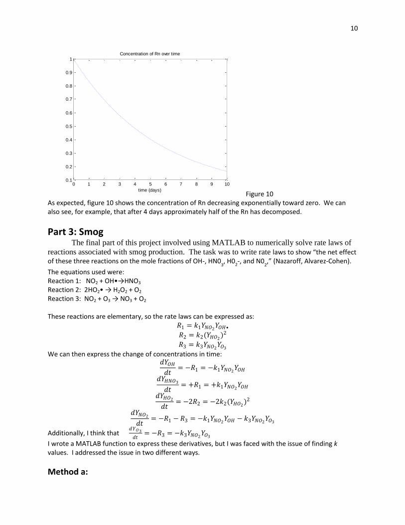
𝐶𝑅𝑛 0 = 𝐶0 From this point, instead of solving analytically, I wrote a MATLAB radon derivative function and used MATLAB to solve the differential equations numerically. I obtained the graph:

10

Figure 10 As expected, figure 10 shows the concentration of Rn decreasing exponentially toward zero. We can also see, for example, that after 4 days approximately half of the Rn has decomposed.

Part 3: Smog The final part of this project involved using MATLAB to numerically solve rate laws of

reactions associated with smog production. The task was to write rate laws to show “the net effect of these three reactions on the mole fractions of OH-, HN0

3, H0

2-, and N0

2,” (Nazaroff, Alvarez-Cohen).

The equations used were: Reaction 1: NO2 + OH•→HNO3 Reaction 2: 2HO2• → H2O2 + O2 Reaction 3: NO2 + O3 → NO3 + O2 These reactions are elementary, so the rate laws can be expressed as:

𝑅1 = 𝑘1𝑌𝑁𝑂2𝑌𝑂𝐻•

𝑅2 = 𝑘2(𝑌𝐻𝑂2)2

𝑅3 = 𝑘3𝑌𝑁𝑂2𝑌𝑂3

We can then express the change of concentrations in time: 𝑑𝑌𝑂𝐻

𝑑𝑡= −𝑅1 = −𝑘1𝑌𝑁𝑂2

𝑌𝑂𝐻

𝑑𝑌𝐻𝑁𝑂3

𝑑𝑡= +𝑅1 = +𝑘1𝑌𝑁𝑂2

𝑌𝑂𝐻

𝑑𝑌𝐻𝑂2

𝑑𝑡= −2𝑅2 = −2𝑘2(𝑌𝐻𝑂2

)2

𝑑𝑌𝑁𝑂2

𝑑𝑡= −𝑅1 − 𝑅3 = −𝑘1𝑌𝑁𝑂2

𝑌𝑂𝐻 − 𝑘3𝑌𝑁𝑂2𝑌𝑂3

Additionally, I think that 𝑑𝑌𝑂3

𝑑𝑡= −𝑅3 = −𝑘3𝑌𝑁𝑂2

𝑌𝑂3

I wrote a MATLAB function to express these derivatives, but I was faced with the issue of finding k values. I addressed the issue in two different ways.

Method a:

0 1 2 3 4 5 6 7 8 9 100.1

0.2

0.3

0.4

0.5

0.6

0.7

0.8

0.9

1Concentration of Rn over time

time (days)

11

I looked online, and found three potential values for k1, k3, and k3. They are: k1 = 1.336 * 1011 k2 = 8.3*105 k3 = 4.284572*107

When using MATLAB’s built-in DE solver, I chose a uniform initial condition of 1

7 mmol for each gas. I

obtained the following results:

Figure 11 Figure 11 shows that OH and NO2 almost instantly reacts away, while HO2 reacts very slowly. As a result of the reaction between OH and NO2, the concentration of HNO3 increases. The relative concentrations of OH and HNO3 appear to be opposite in sign but equal in magnitude. This relationship should not

surprise us, because 𝑑𝑌𝐻𝑁𝑂 3

𝑑𝑡= −

𝑑𝑌𝑂𝐻

𝑑𝑡.

I found my results using my current values of k to be peculiar, because the reaction happened surprisingly quickly.

Method b: I decided to choose arbitrary values of k. First I used k1=k2=k3=1.

figure 12 I noted a few interesting qualities of figure 12:

0 100 200 300 400 500 600 700 800 900 10000

1

2

x 10-4

time

Y

Concentrations of gas over time

NO2

OH

HO2

HNO3

0 100 200 300 400 500 600 700 800 900 10000

1

2

x 10-4

time

Y

Concentrations of gas over time

NO2

OH

HO2

HNO3

12

First, as previously mentioned, HNO3 increases as fast as OH decreases, as illustrated by both the original equations and their rate laws. Also, NO2 was used up much faster than OH, because it has a role in two different reactions. Next, I changed k2 to 2.

Figure 13 Figure 13 shows concentration over time when k1=k2=1 and k2=2. It appears that only the concentration

of HO2 was affected. This makes sense after we look at the differential equations. Only 𝑑𝑌𝐻𝑂 2

𝑑𝑡

incorporates k2. Next, I changed k1 to 4.

Figure 14 Figure 14 shows concentrations over time when k1=4, k2=2, andk3=1. Figure 14 does not look much different than figure 12. However, in figure 14, the concentration of NO2 approaches zero much more rapidly than in figure 12. Furthermore, both OH and HNO3 also seem to react and “level out” faster in

0 100 200 300 400 500 600 700 800 900 10000

1

2

x 10-4

time

Y

Concentrations of gas over time

NO2

OH

HO2

HNO3

0 100 200 300 400 500 600 700 800 900 1000-5

0

5

10

15

20x 10

-5

time

Y

Concentrations of gas over time

NO2

OH

HO2

HNO3

13

figure 14 than in figure 12. Thus, we can see that increasing k values really does increase the rate of a reaction.

14

References Environmental Engineering Science, by William W Nazaroff and Lisa Alvarez-Cohen http://en.wikipedia.org/wiki/Density_of_air “Informal Introduction to Differential Equations” by Chris Brown http://www.atmos-chem-phys.org/10/10521/2010/acp-10-10521-2010-supplement.pdf

http://www.sciencedirect.com/science?_ob=ArticleURL&_udi=B6TFN-3VJ90CF-

5&_user=483663&_coverDate=01%2F11%2F1999&_rdoc=1&_fmt=high&_orig=search&_origin=

search&_sort=d&_docanchor=&view=c&_searchStrId=1568194916&_rerunOrigin=google&_acct

=C000022660&_version=1&_urlVersion=0&_userid=483663&md5=d7496f03fb60af3b81521379

8025b948&searchtype=a

http://uk.answers.yahoo.com/question/index?qid=20100729030905AA8PYj0