1

 Abstract Tile of the document: HVAC system component-based modeling

and implementation Karam H. Rajab

Directed By: Associate Professor Mark Austin Institute for Systems Research and the Department of Civil and Environmental Engineering

The purpose of this scholarly paper is to build the foundation for modeling

components that are used in HVAC systems (heating, ventilation, and air conditioning).

Many models that are currently available are either outdated or do not incorporate certain

capabilities such as unit processing and compatibility. The research done in this paper

utilizes Java and its interface design capability to build components with input and output

ports. In addition to the ports-approach design, it allows each component to have internal

functionality. Such components could transfer physical units between them as well as

apply mathematical functions and evaluating behavioral models to inputs to produce a

certain output for such components. Different Java packages are combined together to

achieve such functionalities.

 

2

HVAC system component-based modeling and implementation By

Karam H. Rajab

Scholarly Paper submitted to the Faculty of the Graduate School of the University of Maryland, College Park, in partial fulfillment of the

Requirements for the degree of Master of Science in Systems Engineering 2013

Advisory Committee: Associate Professor Mark Austin, Chair

3

Table of Contents Table of Figures: ............................................................................................................... 5  CHAPTER 1: INTRODUCTION AND BACKGROUND ............................................ 6  

Interface based design and Block Diagrams ............................................................................ 6  Introduction to HVAC systems ................................................................................................. 7  Simulation Software and HVACSIM+ ..................................................................................... 8  

CHAPTER 2: DATA PROCESSING USING INTERFACES AND COMPONENTS........................................................................................................................................... 11  

Data-Flow Processing between Components ......................................................................... 11  Ports, Components, and wires ................................................................................................. 13  Network of different Physical Expression Processors .......................................................... 13  Part 1. Port Interface Hierarchy and Implementation: Port.java, InputPort.java and OutputPort.java. ...................................................................................................................... 14  Part 2. Component Interface and Base Component Implementation ................................. 15  Part 3. Wire Interface and Implementation .......................................................................... 15  Part 4. Simple Implementation of a MetaComponent .......................................................... 16  Part 5. Component engine/ network assembly: ..................................................................... 17  

CHPATER 3: THE PHYSICS BEHIND THE HVAC NETWORK: ........................ 18  Pump physical Model: ............................................................................................................. 18  Pump implementation in code: ............................................................................................... 20  Pipe physical Model: ................................................................................................................ 20  Pipe implementation in code: ...................................................... Error! Bookmark not defined.  

CHAPTER 5: THE SOFTWARE AND OVERALL NETWORK OF COMPONENTS :............................................................................................................ 24  CHAPTER SIX: CONCLUSION& FUTURE WORK ............................................... 31  REFERENCES: .............................................................................................................. 32  APPENDIX A .................................................................................................................. 34  

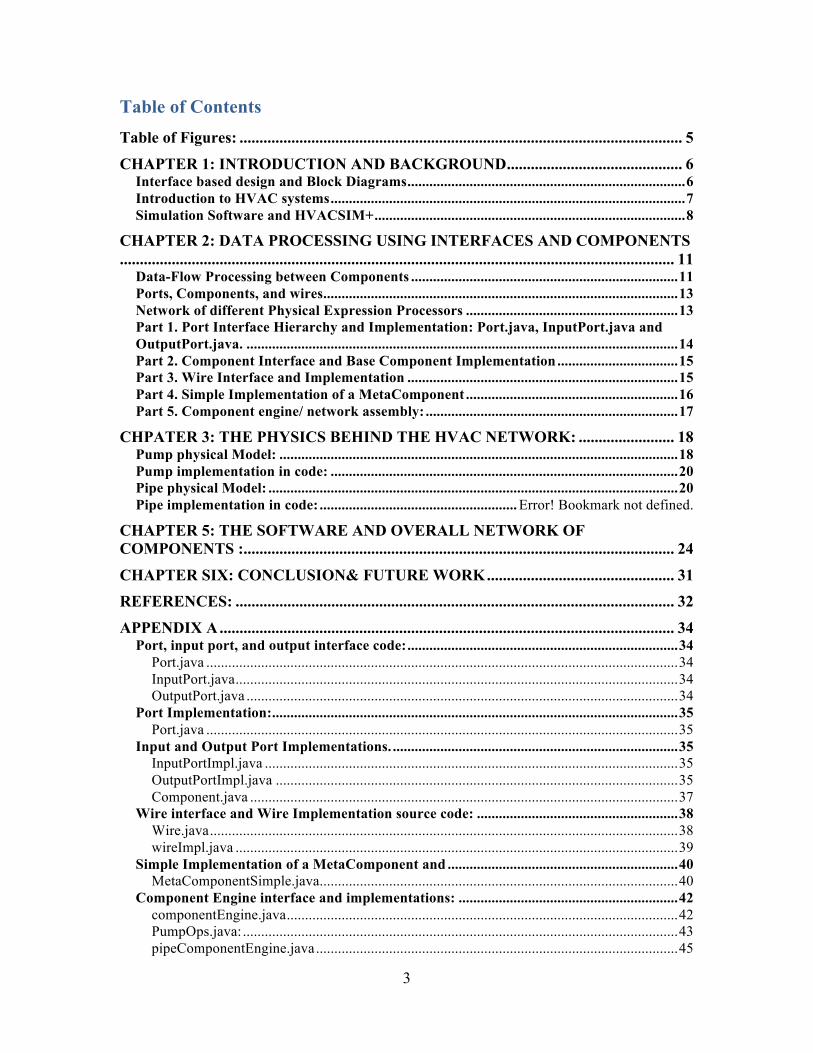
Port, input port, and output interface code: .......................................................................... 34  Port.java ................................................................................................................................. 34  InputPort.java ......................................................................................................................... 34  OutputPort.java ...................................................................................................................... 34  

Port Implementation: ............................................................................................................... 35  Port.java ................................................................................................................................. 35  

Input and Output Port Implementations. .............................................................................. 35  InputPortImpl.java ................................................................................................................. 35  OutputPortImpl.java .............................................................................................................. 35  Component.java ..................................................................................................................... 37  

Wire interface and Wire Implementation source code: ....................................................... 38  Wire.java ................................................................................................................................ 38  wireImpl.java ......................................................................................................................... 39  

Simple Implementation of a MetaComponent and ............................................................... 40  MetaComponentSimple.java .................................................................................................. 40  

Component Engine interface and implementations: ............................................................ 42  componentEngine.java ........................................................................................................... 42  PumpOps.java: ....................................................................................................................... 43  pipeComponentEngine.java ................................................................................................... 45  

4

PipeOps.java: ......................................................................................................................... 45  overall network code: ............................................................................................................... 47  

testnetwork.java ..................................................................................................................... 47  

5

Table of Figures: FIGURE 1: AN OVERALL NETWORK VIEW OF THE COMPONENT MODELING ARCHITECTURE .. 12

FIGURE 2: CLASS DIAGRAM FOR HOW PORTS ARE IMPLEMENTED (AUSTIN) ........................... 14

FIGURE 3: THE ARCHITECTURE OF A DATA PROCESSING UNIT ................................................. 15

FIGURE 4: THE NOTION OF A SOURCE PORT "OUTPUT PORT" AND TARGET PORTS OR "INPUT

PORTS" .................................................................................................................................. 16

FIGURE 5: THE WIRE INTERFACE IMPLEMENTATION ................................................................ 16

FIGURE 6: PUMP CONNECTED TO A PIPE IN A NETWORK (PUMPFUNDAMENTALS) ................... 18

FIGURE 7: PIPE PHYSICAL MODEL REPRESENTATION (EFUNDA) .............................................. 21

FIGURE 8: THE EFFECT OF CHANGING DISCHARGE PRESSURE OF THE PUMP ON PIPE 2'S

OUTPUT PRESSURE ................................................................................................................ 30

6

CHAPTER 1: INTRODUCTION AND BACKGROUND

Interface-based Design and Block Diagrams

Techniques for interface-based systems engineering have emerged in response to

the numerous systems’ failures, and a means to handle complexity that occurred when

involving many stakeholders such as partners and suppliers as well as the huge number of

components used in building systems. It is evident that most of the effort is directed

toward designing individual parts of a system e.g., functionality and tolerances. Interfaces

are often neglected and happen to be in many cases the bottlenecks or the weak points

(De Weck 2009). Another layer of complexity is due to the involvement of many

stakeholders across different fields and locations making it a must to define how

interfaces are designed.

The main objective behind interface-based design is to answer the question:

“What does this component do?” as opposed to “How does the component do it?”. It

focuses less on the functionality of each component, its inputs and outputs, and more

about its overall function (Alfaro 2002). It does this through abstracting components, and

defining them as objects with a common functionality shedding the light on how they

connect together and what they pass to one another.

A very popular type of interface is the physical connection. This connection type

covers many interface types such as mass flow, energy flow, and information flow. A

physical connection exists when two components or more touch each other such as a pipe

and a pump, have a reversible connection between them e.g. USB and cable, or

permanently connected together like rivets (de Weck 2009). This paper will explore this

kind of connections defining a common interface for a category of component or to

model certain parts of the system reduce complexity. A clear interface identification and

definition reduces the risk of failure.

In addition to utilizing interface-based design, a common way that’s used to

model dynamic systems is block diagrams due to its ability to capture all of the essential

information needed to implement some systems. Block diagrams represent concurrent

7

systems using certain semantics. The following is an example of block diagram used in

circuits design to model a first-order differential equation.

Figure 1: a block diagram representing a first order differential equation

Block diagrams are powerful because of their Modularity where large designs are

composed of smaller ones. They’re also hierarchical wherein Composite designs have the

ability to become modules. Third, the ability to function concurrently where

modules/components can logically operate simultaneously. Such implementations may be

sequential or parallel or distributed (Lee 1998). The work done in this paper uses this

notion to build the overall system where components are represented as blocks that could

be then used as a more abstract module composite of smaller ones. The application that

will be used is HVAC systems, which will be discussed in the next section.

Introduction to HVAC systems HVAC (heating, ventilation, and air conditioning) systems design has been

present since the industrial revolution. For most of the 20th century, majority of buildings

did not include such components, and the ones that had such systems were in most cases

discrete, i.e., no interdependency among components. With the emergence of highly

populated skyscrapers and large complex buildings, HVAC systems design has become

mandatory. Moreover, designing HVAC systems focused more on the overall

8

functionality of the different components together as a system with attention paid to

energy efficiency without hindering performance.

Nowadays, the field of HVAC systems design is a subdiscipline of mechanical

engineering, wherein the fundamentals of fluid mechanics, heat transfer, and

thermodynamics govern the conversion, exchange, generation, and use of energy.

Alongside mechanical energy, the role of systems engineering comes into play, when we

deal with different components interacting together as a whole to produce an overall

functionality with certain performance requirements under a certain financial budget.

The ever-continuing search for more energy-efficient building around the globe

has encouraged engineers to focus on the relationship between design variables and

energy performance. Analysis of the energy performance of any HVAC system is

becoming more fundamental in making decisions regarding energy-efficient design

parameters and quantifying the impact of energy conservation measures. Evaluation of

energy characteristics of different design components is becoming a necessity with the

demand for higher efficiency.

Among the many ways to model energy consumption, the best way to optimize

and study how energy is consumed is carried out through creating simulations of building

heating and cooling systems. Not a single energy-efficient building today is constructed

without some form of simulation.

Simulation Software and HVACSIM+ Simulation programs built for research and modeling have been around for many

years, but their advancement into useful tools has not kept up in matching the maturity of

other software frequently used by engineers such as MS Office, CAD, MATLAB, etc.

Examples of some of the lacking areas are: ability to comprehend and process physical

units, user-friendly graphical interfaces, visual representation of components, and many

others. Many HVAC and building-energy analysis applications were developed in

Northern America and Europe. “There are more than two hundred programs available in

[the] USA and over a hundred programs in Europe and elsewhere” (Varanasi, 2002).

Table 1.1 presents a list of a few programs currently being used.

9

Table 1: Software programs used in building HVAC simulation

(Varanasi, 2002, pg. 4)

HVACSIM+, which stands for ‘HVAC Simulation PLUS other systems,’ is a

simulation software package that was developed at the National Institute of Standards and

Technology (NIST), Gaithersburg, Maryland, U.S.A. Its main function is to model

HVAC systems, their controls, the building model, and the other energy management

systems. In this software, the specifications by a user as well as the internal

representation of HVAC elements are represented in terms of single components, e.g.,

fan, duct, heating coil, boiler, pump, and pipe. Such components are then connected

together forming a complete system.

Objective and Scope: Although HVACSIM+ has many useful features, being developed in the mid-

1980s makes it very old, and not very user-friendly. Many efforts have been taken to

upgrade the package, such as the work done by Varanasi (2002). Nonetheless, since it

was developed in ANSI standard Fortran 77, it becomes too old to be revamped (Clark,

1985). The focus of this paper is to build in JAVA a foundation that could be eventually

used to model an overall HVAC system in a sophisticated manner. The scope should

focus on implementing two different components interacting with each other

incorporating physical units processing. This will be built utilizing interface modeling

10

design techniques, which make it easy for expansion, and give the flexibility of

implementing a certain interface with more than one JAVA class.

Chapter two will discuss using interface-based engineering to model different

components. Chapter three will discuss the physics behind pumps and pipes as well as

their implementation in code using the ideas from chapter two. Chapter four will put

everything together from the previous chapters to simulate a network of components

working together.

11

CHAPTER 2: DATA PROCESSING USING INTERFACES AND COMPONENTS

Data-Flow Processing between Components Data processing, as opposed to control flow, is a behavior model defined by

computation within blocks and flow of data between blocks. The model proposed in this

paper is obtained from the code used in engineering software development in Java by

Austin, 2013. His model of “interface specifications and code implementations for a

general purpose, executable, data processing component” code is obtained and further

customized to meet the HVAC system requirements of this project. The basic

components are assembled from wires and ports. The original model is only able to

process only basic data types such as floats, integers, and strings. This model is adopted

and customized to handle actual physical units and quantities. The processing of these

physical quantities and units is driven by a component engine infrastructure. The physical

units definitions used are based on a Java Package called J-science. Moreover, it is a

library that provides a set of Java interfaces for handling units and quantities (Jscience).

The following figure gives an overall idea of hierarchy of J-science as provided by its

developers.

12

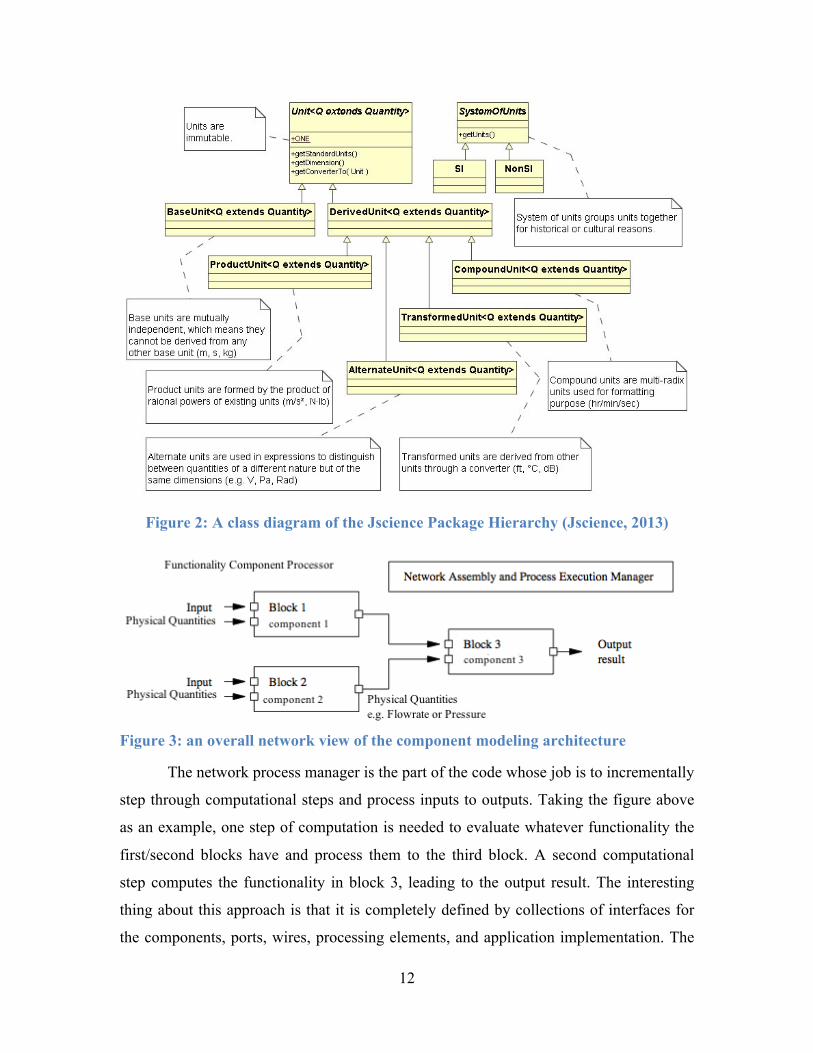
Figure 2: A class diagram of the Jscience Package Hierarchy (Jscience, 2013)

Figure 3: an overall network view of the component modeling architecture

The network process manager is the part of the code whose job is to incrementally

step through computational steps and process inputs to outputs. Taking the figure above

as an example, one step of computation is needed to evaluate whatever functionality the

first/second blocks have and process them to the third block. A second computational

step computes the functionality in block 3, leading to the output result. The interesting

thing about this approach is that it is completely defined by collections of interfaces for

the components, ports, wires, processing elements, and application implementation. The

13

first four parts constitute the main pillars that model a single physical component. The

fifth part, application implementation, puts everything together to build the overall

network of more than components to build an HVAC system like the one in Figure 3.

Ports, Components, and wires The source code is an assembly of 18 files. The code files below are grouped

together based upon whether they implement wire, ports, components, or processing

component. It is important to note that, under each group, we split the files into two

groups, namely, implementation and interface.

Part1: Port Implementation Port Interfaces

PortImpl.java InputPortImpl.java OutputPortImpl.java

port.java InputPort.java OutputPort.java

Table 2: code used to build ports

Part2: Component Implementations Component interface BaseComponent.java Component.java

ComponentEngine.java Table 3: code used to build component

Part3: Wire Implementation Wire Interface WireImpl.java Wire.java

Table 4: code used to build wires

Part4: Management of Data Processing MetaComponentSimple.java

Table 5: code used to process data

It is important to note that the system architecture and the functional capability

are entirely defined by relationships between the various port, components, and wire

interfaces. This is reflected in actual implementations for the port, component, wire and

computational engine classes.

Network of different Physical Expression Processors To demonstrate these capabilities, the five files define a network of different

blocks of “components” processors:

Part5: Application Implementation Use of Interfaces

14

PumpComponentEngine.java PumpOps.java PipeComponentEngine.java PipeOps.java TestNetwork.java

ComponentEngine.java

Table 6: code used to implement the overall application

PumpOps.java is a simple implementation for basic functionality of the pump

operations. PipeOps.java does the same for pipe. PumpComponentEngine.java is the

processing engine that retrieves data values from the incoming ports and calls the Pump

operations processor, and the same goes for PipeComponentEngine.java with respect to

pipe-related data. TestNetwork.java is the code that assembles the component network of

physical processors shown in Figure 1.

Part 1. Port Interface Hierarchy and Implementation: Port.java, InputPort.java and OutputPort.java.

Input and output ports are defined through a two-level hierarchy of interface

definitions as shown in the figure below. For the source code, refer to Appendix A.

Figure 4: Class diagram for how ports are implemented (Austin, 2013)

The port interface depicted above specifies a method for retrieving the component

to which a port belongs using the method getParent() and a simple method for setting the

name of the port. It is interesting to note that the declaration does not mention specific

component implementations. Instead, it refers to the parent component indirectly through

the Component interface implemented by specific components.

15

With respect to input and output port interfaces, they extend (or build upon) the

port interfaces. Input ports set data values and output ports get data values. In our case,

data values are actual physical units.

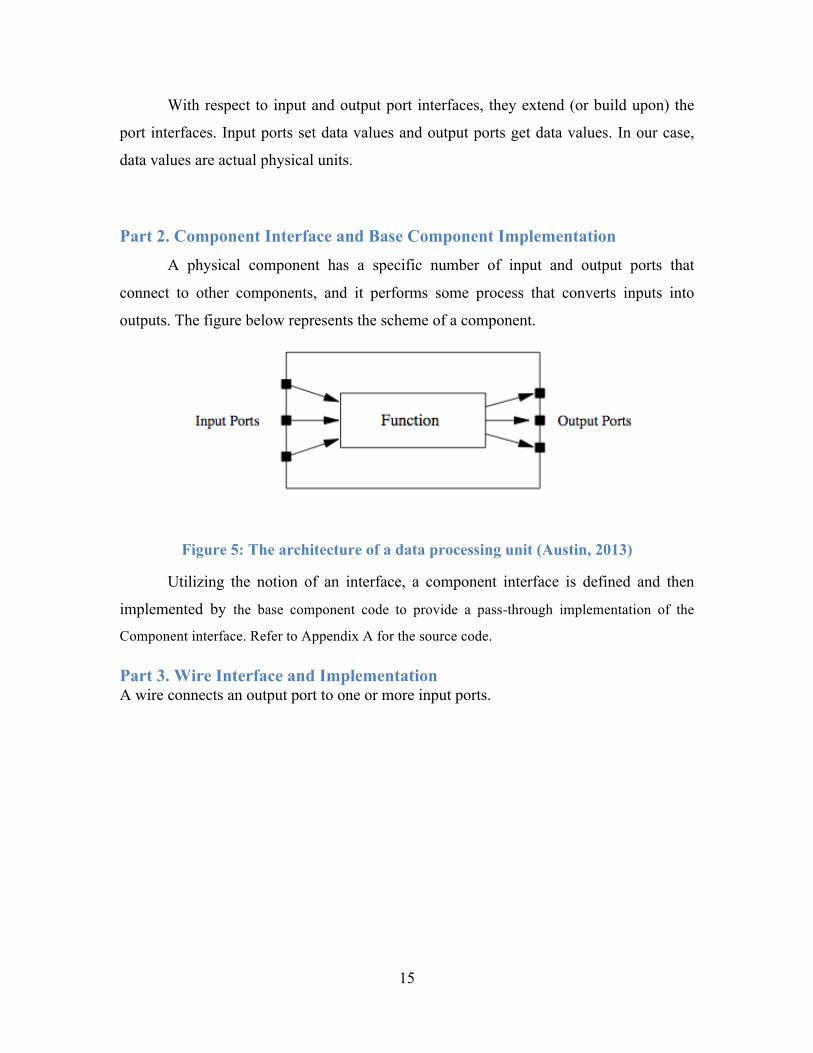
Part 2. Component Interface and Base Component Implementation A physical component has a specific number of input and output ports that

connect to other components, and it performs some process that converts inputs into

outputs. The figure below represents the scheme of a component.

Figure 5: The architecture of a data processing unit (Austin, 2013)

Utilizing the notion of an interface, a component interface is defined and then

implemented by the base component code to provide a pass-through implementation of the

Component interface. Refer to Appendix A for the source code.

Part 3. Wire Interface and Implementation A wire connects an output port to one or more input ports.

16

Figure 6: Notions of a source port "output port" and target ports or "input ports"

The wire interface (wire.java) contains methods for retrieving the source port, the

number of target ports, a specific target port, and a method for propagating data from the

source port to one or more target ports. The wire implementation (wireImpl.java) uses

Array Lists to support the one-to-many relationship between source and destination ports.

The figure below shows that the implementation for the wire interface is done.

Figure 7: The wire interface implementation

Part 4. Simple Implementation of a MetaComponent

This part utilizes a package called JGraphT, a Java graph library that provides

mathematical graph-theory objects and algorithms, to assemble the various components

into a network of processes, and follows a step-by-step process execution of an input-

output relationship of the network. The implementation is “simple” in the sense that the

code in MetaComponentSimple.java does not implement the Component interface.

17

Part 5. Component engine/ network assembly: The class (ComponentEngine.java) defines an interface for the processing engine

of a component. The purpose of the component engine is to convert inputs into outputs.

There are different implementations of this interface. The next section explains and

discusses the different implementations for the functionality of our simple HVAC system.

18

CHPATER 3: THE PHYSICS BEHIND THE HVAC NETWORK:

After examining the model that will allow us to build a simple simulation of some

parts of the HVAC system, this section will discuss the actual components used and their

physical functionality.

To simplify the issue, we are going to model only two components in an HVAC

system. The network to be modeled consists of a pump connected to different pipes. The

main point is to monitor how physical quantities move through the network starting as an

input to a certain component and ending at the end of the network at the output of

another.

We will simplify the analysis by only connecting components in series (no loops)

by pre-determining the direction in which flows will occur. Specifically, in this example,

inputs will only occur at the only one end of the network. i.e., the pump. The inputs to the

pump get calculated and output to the next component in the network, which is a pipe.

The interesting part is to see physical units being transformed within each unit, depending

on its functionality, and processed to the next. The next parts describe the physics and

functionality of each component in the network.

Pump Physical Model: For our component network, the first component modeled was a centrifugal

pump. Its job in simple words is to supply enough discharge pressure to drive the fluid

thought the pipe to the end of the network. Figure 6 below shows basic functionality of

the pump.

Figure 8: Pump connected to a pipe in a network (pump fundamentals)

19

An electrical motor is assumed to be the driver of the pump. The inputs of the pump are

as follows:

-Discharge Pressure (Pd) or the desired pressure at the output of pump. This pressure is the one that will drive the fluid to the end of the pipe. - Suction Pressure (Ps) or the low side pressure is the intake pressure or the pressure of the fluid at the point from where it is being pumped. -Pump Efficiency (ηp) is the ratio of the work or power obtained at the output side of the pump to the amount of power input to the pump. -Pump Efficiency (ηm) is the ratio of the work or power obtained at the output side of the electrical motor driving the pump to the amount of power input to the motor. -Electrical power (W) supplied to the pump. -The diameter (D) of the pipe connected.

The output obtained is the flow rate of the fluid (Q). However, since the flowrate

controls the velocity of the fluid in the pipe and the latter depends on the diameter of

pipe, the actual output is the fluid velocity. To examine how the flowrate (Q) is

calculated, the following expression is used:

𝒇𝒍𝒐𝒘𝒓𝒂𝒕𝒆 ∗∗ 𝑸 𝑚!s =  

𝛈𝒑 % ∗ 𝛈𝒎 % ∗ 𝑾 Watt𝑷𝒅 Atm − 𝑷𝒔 Atm

After calculating the flowrate from the inputs values, the pump calculates the

fluid velocity, which is output to the pipe based upon the following relation.

𝒇𝒍𝒖𝒊𝒅  𝒗𝒆𝒍𝒐𝒄𝒊𝒕𝒚  (𝑽) =  𝑸 𝑚!

s ∗ 4�𝑫� m! ∗ π

It is important to note that we assume the pipe is circular and that we are taking

the input values at the same pump conditions, i.e., flow, pressures, and speed.

20

Pump Component Model: After examining the physics behind the pump component, it is now easy to

understand how this component is implemented in code. At the end of the previous

chapter, we examined the interface componentEngine.java. However, the implementation

of this component engine was not explained. Since the componentEngine.java class is an

interface, it can be implemented in many ways depending on the specific component that

is modeled. The code in PumpComponentEngine.java in the appendix explains how it is

implemented. The operations or function within the pump is implemented in the class

PumpOps.java. The following figure shows a block diagram of a single pump

component. The overall flow of the code will be explained in the next chapter.

Figure 9: A pump block diagram

Pipe physical Model: The second component modeled is a horizontal pipe running from Point A to Point B.

The pipe is assumed to be relatively straight with no sharp bends. This assumption is

served by the fact that changes in pressure will be mostly due to elevation changes

friction with the pipe walls. The model is based on Engineering Fundamentals (efunda).

21

Figure 10: Pipe Physical model Representation (efunda)

The inputs of the pipe are:

-Fluid velocity (V), which is input by the previous component, e.g., a pump or previous

pipe.

-Pressure input (Pa) or the pressure of the fluid at the output of the previous component at

component A as show above in the figure.

-Pipe Diameter (D) explained above.

-Pipe Relative Roughness, which depends on the pipe material and its diameter.

-Pipe Length (L) as shown on the previous figure.

-Pipe Elevation (Δz), which represents the height difference between the input and the

output point as the figure, shows.

-Fluid Density (ρ)

-Fluid viscosity (µ)

It’s assumed that the pipe diameter (D) is constant, leading to a constant flow. This leads to the following expression using Bernoulli’s equation:

𝑃𝑏[Pa] =  𝑃𝑎[Pa]−  𝜌[kg

𝑚!] ∗ 𝑔[m 𝑠!] ∗ Δz[m]+ 𝑓[𝑑𝑖𝑚𝑒𝑛𝑠𝑖𝑜𝑛𝑙𝑒𝑠𝑠]𝐿[m]𝐷[m]

𝑉![𝑚!

𝑠!]2𝑔[m 𝑠!]

It is important to note that this only applies for constant flow and constant fluid

velocity.

The friction factor (f) depends on the Reynolds Number (R). In the model built, we only

consider laminar flow for the sake of simplicity. The Reynolds number for laminar flow

22

is calculated as:

𝑅 𝑑𝑖𝑚𝑒𝑛𝑠𝑖𝑜𝑛𝑙𝑒𝑠𝑠 =𝜌 kg

𝑚! ∗ 𝑉 m s ∗ 𝐷 m

𝜇 𝑘𝑔𝑚∗𝑠

For laminar flow (R < 2000 in pipes), f can be deduced analytically. The answer is,

𝑓 𝑑𝑖𝑚𝑒𝑛𝑠𝑖𝑜𝑛𝑙𝑒𝑠𝑠 =64𝑅

Thus, the component first calculates the Reynolds number followed by friction factor. It

then, uses f to calculate pressure at point b.

Pipe Component Model: After examining the physics behind the pipe component, the implementation of the pipe

component follows exactly the way the pump modeled. Figure below shows a diagram of

a pipe model. The code in PipeComponentEngine.java class implements the

ComponentEngine.java interface. The operations or function within the pipe explained

above is implemented in the class PipeOps.java. The next section explains the network

overall.

Figure 11: Pipe block Diagram

23

24

CHAPTER 4: THE SOFTWARE AND OVERALL NETWORK OF COMPONENTS:

This part of the paper will put the pieces discussed above together in one image.

The code below starts by defining a pump component with 6 inputs and 1 output. In

addition, it defines a pipe with 8 inputs and 2 outputs.

public class TestNetwork { //============================================== //Create a (pump) component .... //============================================== public static Component<Amount<?>> createPump( int inputs) { PumpOps add = new PumpOps (6, 1); add.setOpsType ( PumpOps.FLOWRATE ); add.setName ( "FLOWRATE" ); PumpComponentEngine processor = new PumpComponentEngine(add); BaseComponent<Amount<?>> bc = new BaseComponent<Amount<?>>(inputs, 1, processor); return ( bc ); } //============================================== //Create a (pipe) component .... //============================================== public static Component<Amount<?>> createPipe( int inputs) { PipeOps ops = new PipeOps (8, 2); ops.setOpsType ( PipeOps.PRESSURE ); ops.setName ( "PRESSURE" ); PipeComponentEngine processor = new PipeComponentEngine(ops); BaseComponent<Amount<?>> bc = new BaseComponent<Amount<?>>(inputs, 2, processor); return ( bc ); }

After defining the components in the network, a network components manager is

created that will be responsible for connecting the outputs and inputs of the different

components together in order to be able to pass physical quantities. We then create

instances of each component, name them, and assign their inputs and ports. After

assigning inputs and output ports, the physical values for these inputs are then set.

After configuring input values for the components, the connection between the

different components was then set. The code below connects pump1 to pipe1. Then, print

the values at each input port for the system were set, and connecting components in the

system as show in part 3 after propagating the signal continues. Part 4, 5 just print out the

results after quantities have been propagated throughout the network.

25

//============================================== //Assemble and Exercise component assembly .... //============================================== public static void main(String[] args) { System.out.println("In NetworkTest.main() ... "); //Create network manager .... MetaComponentSimple<Amount<?>> manager = new MetaComponentSimple<Amount<?>>(); //create Pump component ... Component<Amount<?>> pump1 = null ; pump1 = createPump( 6); pump1.setName("pump 1"); //Create Pipe components ... Component<Amount<?>> pipe1 = null ; pipe1 = createPipe( 8); pipe1.setName("pipe 1"); Component<Amount<?>> pipe2 = null; pipe2 = createPipe( 8); pipe2.setName("pipe 2"); //assign input ports for pump 1..... InputPort<Amount<?>> pressureDischarge = pump1.getInputPort(0); InputPort<Amount<?>> pressureSuction = pump1.getInputPort(1); InputPort<Amount<?>> ePower = pump1.getInputPort(2); InputPort<Amount<?>> pDiamater = pump1.getInputPort(3); InputPort<Amount<?>> motorEffeciency = pump1.getInputPort(4); //pump attributes as inputs InputPort<Amount<?>> pumpEffeciency = pump1.getInputPort(5); //Set the input values for pump1 pressureDischarge.setValue(Amount.valueOf(300, ATMOSPHERE)); pressureSuction.setValue(Amount.valueOf(299.9,ATMOSPHERE)); ePower.setValue(Amount.valueOf(3000, WATT)); pDiamater.setValue(Amount.valueOf(3, METRE)); motorEffeciency.setValue(Amount.valueOf(.5, WATT.divide(WATT)) ); pumpEffeciency.setValue(Amount.valueOf(.5, WATT.divide(WATT)));

26

//assign input ports for pipe 1..... InputPort<Amount<?>> inletPressure = pipe1.getInputPort(0); InputPort<Amount<?>> fluidVelocity = pipe1.getInputPort(1); InputPort<Amount<?>> fluidDensity = pipe1.getInputPort(2); InputPort<Amount<?>> fluidViscosity = pipe1.getInputPort(3); //pipe attributes as inputs InputPort<Amount<?>> pRoughness = pipe1.getInputPort(4); InputPort<Amount<?>> pLength = pipe1.getInputPort(5); //pDiameter is defined as it's required as an input for the pump connecting to this pipe pDiamater = pipe1.getInputPort(6); //pElevation = difference between input and output in elevation ... InputPort<Amount<?>> pElevation = pipe1.getInputPort(7); //Set the input values for pipe1 inletPressure.setValue( Amount.valueOf(500, ATMOSPHERE) ) ; //fluidVelocity.setValue( Amount.valueOf(1, METRE_PER_SECOND) ); fluidDensity.setValue( Amount.valueOf(1, KILOGRAM.divide(CUBIC_METRE)) ); fluidViscosity.setValue( Amount.valueOf(0.5, KILOGRAM.divide(SECOND).divide(METRE))); pRoughness.setValue( Amount.valueOf(.005, METRE.divide(METRE))); pLength.setValue( Amount.valueOf(5, METRE)); pDiamater.setValue(Amount.valueOf(3, METRE)); pElevation.setValue( Amount.valueOf(1, METRE)); //assign input ports for pipe 2..... //fluidVelocity = pipe2.getInputPort(1); fluidDensity = pipe2.getInputPort(2); fluidViscosity = pipe2.getInputPort(3); pRoughness = pipe2.getInputPort(4); pLength = pipe2.getInputPort(5); pDiamater = pipe2.getInputPort(6); pElevation = pipe2.getInputPort(7); //set input values for pipe 2: //fluidVelocity.setValue( Amount.valueOf(1, METRE_PER_SECOND) ); fluidDensity.setValue( Amount.valueOf(1, KILOGRAM.divide(CUBIC_METRE)) ); fluidViscosity.setValue( Amount.valueOf(0.5, KILOGRAM.divide(SECOND).divide(METRE))); pRoughness.setValue( Amount.valueOf(.005, METRE.divide(METRE))); pLength.setValue( Amount.valueOf(60, METRE)); pDiamater.setValue( Amount.valueOf(15, SI.CENTIMETER)); pElevation.setValue( Amount.valueOf(200, METRE)); //Assemble graph of processing components ... manager.connect( pump1.getOutputPort(0), pipe1.getInputPort(1) ); //Print details of components at beginning of propogation ... System.out.println( ""); System.out.println( "Part 1: Initial Condition of Base Components ... "); System.out.println( "------------------------------------------------ "); System.out.println( pump1.toString() ); System.out.println( pipe1.toString() ); System.out.println( pipe2.toString() ); //Print details of meta-component graph ... System.out.println( ""); System.out.println( "Part 2: Meta-Component Graph ... "); System.out.println( "----------------------------------- "); //System.out.println( manager.getGraph().toString() ); //Propogate signals through component wires ... System.out.println( ""); System.out.println( "Part 3: Propogate signals: Steps 1 and 2... "); System.out.println( "------------------------------------------- "); manager.process(); manager.process(); manager.connect( pipe1.getOutputPort(0), pipe2.getInputPort(0) ); manager.connect( pipe1.getOutputPort(1), pipe2.getInputPort(1) ); manager.process(); manager.process();

27

//Print details of meta-component graph ... System.out.println( ""); System.out.println( "Part 4: Meta-Component Graph ... "); System.out.println( "----------------------------------- "); System.out.println( pipe1.toString() ); System.out.println( "just printed part 1 ... "); System.out.println( "... ... "); System.out.println( "... ... "); System.out.println( "... ... "); System.out.println( pipe2.toString() ); System.out.println( "just printed part 2 ... ");

System.out.println( ""); System.out.println( "Part 5: Result .... "); System.out.println( "----------------------------------- "); OutputPort<Amount<?>> y ; // dummy for output values InputPort<Amount<?>> z ; // dummy for input values. System.out.println( "PUMP 1 results" ); for(int i=0; i<5; i++){ z = pump1.getInputPort(i); System.out.println( "Answer: pump 1 inputPort ["+i+"] = " + z.getValue() ); } for(int i=0; i <1; i++){ y = pump1.getOutputPort(i); System.out.println( "Answer: pump 1 OutPort ["+i+"] = " + y.getValue() ); } //pipes System.out.println( "PIPE 1 results" ); for(int i=0; i <8; i++){ z = pipe1.getInputPort(i); System.out.println( "Answer: pipe 1 inputPort ["+i+"] = " + z.getValue() ); } for(int i=0; i <2; i++){ y = pipe1.getOutputPort(i); System.out.println( "Answer: pipe 1 OutPort ["+i+"] = " + y.getValue() ); } System.out.println( "PIPE 2 results" ); for(int i=0; i <8; i++){ z = pipe2.getInputPort(i); System.out.println( "Answer: pipe 2 inputPort ["+i+"] = " + z.getValue() ); } for(int i=0; i <2; i++){ y = pipe2.getOutputPort(i); System.out.println( "Answer: pipe 2 OutPort ["+i+"] = " + y.getValue() ); } System.out.println( "... ... "); } }

The following graphs shows basically the different components in the network connected together:

28

Figure 12: the overall network of components connected in series

The following is the output we get when running the code: In NetworkTest.main() ... Part 1: Initial Condition of Base Components ... ------------------------------------------------ component(pump 1) Inputs: 300 atm (299.89999999999998 ? 2.8E-14) atm 3000 W 3 m (0.5 ? 2.8E-17) (0.5 ? 2.8E-17) Outputs1: null component(pipe 1) Inputs: 300 atm null 1 kg/m? (0.5 ? 2.8E-17) kg/(s?m) (0.0049999999999999992 ? 4.3E-19) 5 m 3 m 1 m Outputs1: null null component(pipe 2) Inputs: null null 1 kg/m? (0.5 ? 2.8E-17) kg/(s?m) (0.0049999999999999992 ? 4.3E-19) 60 m 15 cm 200 m Outputs1: null null Part 2: Meta-Component Graph ... ----------------------------------- Part 3: Propogate signals: Steps 1 and 2... ------------------------------------------- Part 4: Meta-Component Graph ... ----------------------------------- component(pipe 1) Inputs: 300 atm (0.010471581090012 ? 3.0E-15) m/s 1 kg/m? (0.5 ? 2.8E-17) kg/(s?m) (0.0049999999999999992 ? 4.3E-19) 5 m 3 m 1 m Outputs1: (299.99990229725415 ? 2.8E-14) atm (1.1137197067 ? 3.2E-10) m/s just printed part 1 ... ... ... ... ... ... ... component(pipe 2) Inputs: (299.99990229725415 ? 2.8E-14) atm (1.1137197067 ? 3.2E-10) m/s 1 kg/m? (0.5 ? 2.8E-17) kg/(s?m) (0.0049999999999999992 ? 4.3E-19) 60 m 15 cm 200 m Outputs1: (299.5115722949 ? 4.1E-10) atm (1.1596883785 ? 9.7E-10) m/s just printed part 2 ...

29

Part 5: Result .... ----------------------------------- PUMP 1 results Answer: pump 1 inputPort [0] = 300 atm Answer: pump 1 inputPort [1] = (299.89999999999998 ? 2.8E-14) atm Answer: pump 1 inputPort [2] = 3000 W Answer: pump 1 inputPort [3] = 3 m Answer: pump 1 inputPort [4] = (0.5 ? 2.8E-17) Answer: pump 1 OutPort [0] = (0.010471581090012 ? 3.0E-15) m/s Answer: pump 1 OutPort [1] = 300 atm PIPE 1 results Answer: pipe 1 inputPort [0] = 300 atm Answer: pipe 1 inputPort [1] = (0.010471581090012 ? 3.0E-15) m/s Answer: pipe 1 inputPort [2] = 1 kg/m? Answer: pipe 1 inputPort [3] = (0.5 ? 2.8E-17) kg/(s?m) Answer: pipe 1 inputPort [4] = (0.0049999999999999992 ? 4.3E-19) Answer: pipe 1 inputPort [5] = 5 m Answer: pipe 1 inputPort [6] = 3 m Answer: pipe 1 inputPort [7] = 1 m Answer: pipe 1 OutPort [0] = (299.99990229725415 ? 2.8E-14) atm Answer: pipe 1 OutPort [1] = (1.1137197067 ? 3.2E-10) m/s PIPE 2 results Answer: pipe 2 inputPort [0] = (299.99990229725415 ? 2.8E-14) atm Answer: pipe 2 inputPort [1] = (1.1137197067 ? 3.2E-10) m/s Answer: pipe 2 inputPort [2] = 1 kg/m? Answer: pipe 2 inputPort [3] = (0.5 ? 2.8E-17) kg/(s?m) Answer: pipe 2 inputPort [4] = (0.0049999999999999992 ? 4.3E-19) Answer: pipe 2 inputPort [5] = 60 m Answer: pipe 2 inputPort [6] = 15 cm Answer: pipe 2 inputPort [7] = 200 m Answer: pipe 2 OutPort [0] = (299.5115722949 ? 4.1E-10) atm Answer: pipe 2 OutPort [1] = (1.1596883785 ? 9.7E-10) m/s ... ...

A package called jmathPlot is used to plot the effect of changing the input of the pump to

the output of the pipes. In the example below, the desired discharge pressure of the pump

is changed over a certain range to monitor how that affects the output pressure of pipe 2:

30

Figure 13: the effect of changing Discharge pressure of the pump on Pipe 2's output pressure

31

CHAPTER 6: CONCLUSION& FUTURE WORK

It can be seen how physical quantities flow through the different components.

Each component transfer function changes the input to appropriate outputs depending on

its properties. Such a model could be used in the future to model energy consumption

overtime. Additionally, it could be incorporated with more sophisticated algorithms

including differential equations to model more realistic systems. The proposed model

serves as a basic foundation for simulating HVAC component. It utilizes component-

based modeling, interface-based modeling, and abstractions to simplify the change of

pressure across a 3-component HVAC simple system. In addition to the suggested

improvement mentioned above, the graphical interface could be improved to

accommodate for more control as well as user-friendliness.

32

REFERENCES:

• Austin, Mark. "12 Modeling Abstractions and Software Design Patterns." Reading.

United States, College Park. Mar. 2013. Engineering Software Development in Java.

College Park: ISR, 2013. 156-224. Print.

• Clark, Daniel R., and William B. May. HVACSIM+ Building Systems and

Equipment Simulation Program: Users Guide. Gaithersburg, MD: U.S. Dept. of

Commerce, National Bureau of Standards, 1985. Print. • Clark, D. R. HVACSIM+ Building Systems and Equipment Simulation Program

Reference Manual. NBSIR 84-2996. National Bureau of Standards, January, 1985.

• Dautelle, Jean-Marie. Jscience. Computer software. Jscience. Vers. 4.3. N.p., 2011.

Web. 8 Apr. 2013. <http://jscience.org/>. • De Weck, Olivier. "Systems Integration and Interface Management." Lecture.

Fundamentals of Systems Engineering. Massachusetts, Cambridge. 30 Oct. 2009.

N.p.: n.p., n.d. Print.

• Varnasi, Aditya. Development Of A Visualtoolfor HVACSIM+. Thesis. Oklahoma

State University, 2002. N.p.: n.p., n.d. Print.

• De, Alfaro Luca., and Thomas A. Henzinger. "Interface Theory Component Based

Design." Engineering Theories of Software Intensive Systems: International Summer

School Marktoberdorf August 3 to August 15, 2004; Working Material for the

Lectures. München: Inst. F. Informatik TUM, 2004. N. pag. Print.

• Lee, Edward A. "Block Diagrams for Modeling and Design." Lecture. UC Berkeley.

Dept. of EECS, Berkeley. 2002. N.p.: n.p., n.d. Print.

• Naveh, Barak. JGraphT. Computer software. JGraphT. Vers. 0.8.3. SourceForge,

n.d. Web. 8 Apr. 2013.

33

• "CENTRIFUGAL PUMP SYSTEM TUTORIAL." HOW TO Design a Pump

System. N.p., n.d. Web. 09 Apr. 2013.

<http://www.pumpfundamentals.com/tutorial2.htm>.

34

APPENDIX A

Port, input port, and output interface code:

Port.java package component; publicinterface Port<T> { public Component<T> getParent(); }

*************************************************************

InputPort.java Public interface InputPort<T>extends Port<T> { Public void setName(String sName); Public void setValue(T value); public T getValue(); }

*************************************************************

OutputPort.java Public interface OutputPort<T>extends Port<T> { Public void setName(String sName); public T getValue(); }

*************************************************************

35

Port Implementation:

Port.java =============================================================== * A base for building port implementations. It can function * either as an input or output port, or both. * * @see com.wickedcooljava.sci.component.InputPortImpl * @see com.wickedcooljava.sci.component.OutputPortImpl * =============================================================== package component; import org.jscience.physics.amount.*; public class PortImpl<T>implements Port<T> { private Boolean initialized = false; private String sName; private Component<T>parent; private T value; public PortImpl(Component<T> par) { parent = par; } public Component<T> getParent() { return parent; } Public void setName( String sName ) { this.sName = sName; } Public void setValue(T val) { this.initialized = true; value = val; } publicvoid setValue(PortImpl<Amount<?>> arg1) { this.initialized = true; value = (T) arg1; } public T getValue() { return value; } Public boolean getInitialized() { Return this.initialized; } public String toString() { return"\n" + sName + ".value=" + value; } }

*************************************************************

Input and Output Port Implementations.

InputPortImpl.java package component; public class InputPortImpl<T>extends PortImpl<T>implements InputPort<T> { public InputPortImpl(Component<T> parent) { super(parent); } }

*************************************************************

OutputPortImpl.java

36

Public class OutputPortImpl<T>extends PortImpl<T>implements OutputPort<T> { public OutputPortImpl(Component<T> parent) { super(parent); } }

*************************************************************Component interface and Base Component Implementation definitions:

37

Component.java =========================================================== Component.java: A generic interface for components that process any type of data. * =========================================================== package component; public interface Component<T> { /// set component name ... Public void setName( String sName ); /// get the number of input ports publicint getInputSize(); /// get the number of output ports publicint getOutputSize(); /// get the nth input port public InputPort<T> getInputPort(int index); ///get the nth output port public OutputPort<T> getOutputPort(int index); /// perform the component's processing publicvoid process(); }

************************************************************* Base Component Implementation package component; publicclass BaseComponent<T>implements Component<T> { protected String sName; protectedintinSize, outSize; protected InputPortImpl<T>[] inports; protected OutputPortImpl<T>[] outports; // the function performed by this component protected ComponentEngine<T>function; /** * * @param inputs Number of input ports * @param outputs Number of output ports * @param f The function to perform the processing */ public BaseComponent(int inputs, int outputs, ComponentEngine<T> f ) { inSize = inputs; outSize = outputs; function = f; inports = new InputPortImpl[inSize]; for (int i = 0; i <inSize; i++) { inports[i] = new InputPortImpl<T>(this); } outports = new OutputPortImpl[outSize]; for (int i = 0; i <outSize; i++) { outports[i] = new OutputPortImpl<T>(this); } } public void setName ( String sName ) { this.sName = sName; for (int i = 0; i <inSize; i++) { inports[i].setName("component(" + sName + ").in[" + i + "]"); } for (int i = 0; i <outSize; i++) { outports[i].setName("component(" + sName + ").out[" + i + "]");

38

} } public int getInputSize() { return inSize; } public int getOutputSize() { return outSize; } public InputPort<T> getInputPort(int index) { return inports[index]; } public OutputPort<T> getOutputPort(int index) { return outports[index]; } /** * Delegate to the engine to do the processing. */ public void process() { function.process(inports, outports); } // Detailed string representation .... public String toString() { StringBuffer buf = new StringBuffer(); buf.append("component(" + sName + ")"); buf.append(" Inputs: "); for (PortImpl port : inports) { buf.append(port.getValue()); buf.append(" "); } buf.append(" Outputs1: "); for (OutputPort port : outports) { buf.append(port.getValue()); buf.append(" "); } return buf.toString(); } }

*************************************************************

Wire interface and Wire Implementation source code:

Wire.java /** * A wire that connects an output port to one or more input ports. */ package component; publicinterface Wire<T> { public OutputPort<T> getSourcePort(); publicint getNumberOfTargetPorts(); public InputPort<T> getTargetPort(int index); publicvoid propagateSignal(); }

*************************************************************

39

wireImpl.java package component; import java.util.ArrayList; public class WireImpl<T> implements Wire<T> { private OutputPort<T>source; // lazy target array private ArrayList<InputPort<T>>targetList; private InputPort<T>target; private int count = 0; public WireImpl(OutputPort<T> src) { source = src; } public OutputPort<T> getSourcePort() { return source; } public int getNumberOfTargetPorts() { return count; } public InputPort<T> getTargetPort(int index) { if (index >= count || index < 0) { throw new IndexOutOfBoundsException(); } if (target != null) { return target; } return targetList.get(index); } public void addTargetPort(InputPort<T> tgt) { if (targetList == null) { if (target == null) { target = tgt; count++; } else { targetList = new ArrayList<InputPort<T>>(); targetList.add(target); target = null; } } if (targetList != null) { if (!targetList.contains(tgt)) { targetList.add(tgt); count++; } } } public void propagateSignal() { T value = source.getValue(); if (target == null) { if (targetList != null) { for (InputPort<T> tgt : targetList) { tgt.setValue(value); } } } else { target.setValue(value); } } }

40

Simple Implementation of a MetaComponent and

MetaComponentSimple.java /** * ====================================================================== * MetaComponentSimple.java: This is a simple version of a MetaComponent. * * It uses jgrapht to maintain the connections between child components. * * Original Code: Wicked Cool Java book. * Modified by: Mark Austin October 2009 * ====================================================================== */ package component; import org.jgraph.*; import org.jgraph.graph.*; import org.jgrapht.*; import org.jgrapht.ext.*; import org.jgrapht.graph.*; import org.jgrapht.ListenableGraph; import org.jgrapht.ext.JGraphModelAdapter; import org.jgrapht.graph.ListenableDirectedGraph; // Setup default edge import org.jgrapht.graph.DefaultEdge; public class MetaComponentSimple<T> { // the graph that maintains child components private ListenableDirectedGraph graph; public MetaComponentSimple() { graph = new ListenableDirectedGraph<T,DefaultEdge>(DefaultEdge.class); } // =================================================================== // Connect an output port to an input port. // =================================================================== public void connect( OutputPort<T> out, InputPort<T> in ) { Component<T> source = out.getParent(); Component<T> target = in.getParent(); // 1: Add parent components to graph if (graph.containsVertex(source) != true) { graph.addVertex(source); } if (graph.containsVertex(target) != true) { graph.addVertex(target); } // 2: Add ports to graph if (graph.containsVertex(in) != true ) { graph.addVertex(in); } if (graph.containsVertex(out) != true) { graph.addVertex(out); } // 3: Add an edge from out parent to output port

41

graph.addEdge(source, out); // 4: Add an edge from output port to input port graph.addEdge(out, in); // 5: add an edge from input port to target component graph.addEdge(in, target); }

42

// =================================================================== // Perform the processing by processing each of the subcomponents // and propagating signals from outputs to inputs. // =================================================================== public void process() { processSubComponents(); propagateSignals(); } // =================================================================== // For all connected sub componets, propagate signals from all outputs // to all inputs. // =================================================================== private void propagateSignals() { // Walk along edges and propogate output port values to // input port values .... for (Object item : graph.edgeSet()) { DefaultEdge edge = (DefaultEdge) item; Object source = graph.getEdgeSource( edge ); Object target = graph.getEdgeTarget( edge ); if (source instanceof OutputPort) { OutputPort<T> out = (OutputPort<T>) source; InputPort<T> in = (InputPort<T>) target; in.setValue( out.getValue() ); } } } // ================================================================= // Process all subcomponents, by calling the process methods for each. // ================================================================= private void processSubComponents() { for (Object item : graph.vertexSet()) { if (item instanceof Component) { ((Component<T>) item).process(); } } } // ================================================================= // Returns the graph used by this MetaComponent // ================================================================= public Graph getGraph() { return graph; } }

Component Engine interface and implementations:

componentEngine.java /** * ====================================================================== * An interface for the processing engine of a component. * Its job is to convert inputs into outputs. * Note: This is a kind of functor but does not follow the JGA convention. * ====================================================================== */ package component; public interface ComponentEngine<T> { public void process( PortImpl<T>[] in, PortImpl<T>[] out ); } *************************************************************

43

PumpComponentEngine.java package demo.testnetwork; import org.jscience.physics.amount.Amount; import component.*; /** * A Unit Component which operates using physical ..... */ public class PumpComponentEngine implements ComponentEngine<Amount<?>> { private PumpOps tt; public PumpComponentEngine( PumpOps ops ) { tt = ops; } public void process( PortImpl<Amount<?>>[] in, PortImpl<Amount<?>>[] out ) { PortImpl<Amount<?>> arg1 = in[0]; // number of input ports PortImpl<Amount<?>> arg2 = in[1]; PortImpl<Amount<?>>[] input_buffer = null; input_buffer = in; PortImpl<Amount<?>>[] output_buffer = null; int outLength = out.length; int i =0; if( arg1.getInitialized() == true && arg2.getInitialized() == true ) { Amount<?>[] value = tt.computeValue ( outLength, input_buffer ); output_buffer = out; for (i= 0; i< outLength; i++){ output_buffer[i].setValue( value[i]); } } } }

*************************************************************

PumpOps.java:

44

package demo.testnetwork; import javax.measure.quantity.*; import javax.measure.unit.SI; import javolution.lang.MathLib; import org.jscience.physics.amount.*; import component.PortImpl; /** * A simple pump operations implementation .... */ public class PumpOps { private String name; private PumpOps ops; // Details of pump operation .... public static final PumpOps FLOWRATE = new PumpOps("FLOW_RATE"); // ======================================================================= // Create arithmetic operations object with the specified number of args.. // ======================================================================= public PumpOps(int inputs, int outputs) { this.name = null; } public PumpOps( String name ) { this.name = name; } public void setOpsType ( final PumpOps ops ) { this.ops = ops; } public void setName ( String name ) { this.name = name; } public String getName() { return this.name; } public PumpOps getOps() { return this.ops; } public Amount<?>[] computeValue ( int n, PortImpl<Amount<?>>[] in) { int inLength = n; Amount<?>[] args = new Amount<?>[in.length] ; for (int i = 0; i < in.length; i++) { args[i] = in[i].getValue() ; } Amount<?>[] value = new Amount<?>[inLength] ; for (int i = 0; i < inLength; i++) { value[i] = null ; } if ( PumpOps.FLOWRATE == this.getOps() ) { Amount<?> pressDiff = args[0].minus(args[1]); System.out.println(" pressDiff" + pressDiff); Amount<?>X = args[4].times(args[5]).times(args[2]).times(2298).divide(pressDiff); Amount<VolumetricFlowRate> flowrate= (Amount<VolumetricFlowRate>) X.to(SI.CUBIC_METRE.divide(SI.SECOND)); System.out.println(" flowrate" + flowrate); Amount<?> Y = flowrate.times(4).divide(Math.PI).divide(args[3].pow(2)); Amount<Velocity> fluidVelocity =(Amount<Velocity>) Y.to(SI.METERS_PER_SECOND); value[0]= fluidVelocity; } else { System.out.println("*** Arithmetic Operation Type not defined .. "); }

45

return value; } public String toString() { String s = "PipeOps: type = " + this.name + "\n"; return s; } } *************************************************************

pipeComponentEngine.java package demo.testnetwork; import org.jscience.physics.amount.Amount; import component.*; /** * A Unit Component which operates using physical ..... */ public class PipeComponentEngine implements ComponentEngine<Amount<?>> { private PipeOps tt; public PipeComponentEngine( PipeOps pOps ) { tt = pOps; } public void process( PortImpl<Amount<?>>[] in, PortImpl<Amount<?>>[] out ) { PortImpl<Amount<?>> arg1 = in[0]; PortImpl<Amount<?>> arg2 = in[1]; PortImpl<Amount<?>>[] input_buffer = null; input_buffer = in; PortImpl<Amount<?>>[] output_buffer = null; int outLength = out.length; int i =0; if( arg1.getInitialized() == true && arg2.getInitialized() == true ) { Amount<?>[] value = tt.computeValue ( outLength, input_buffer ); output_buffer = out; for (i= 0; i< outLength; i++){ output_buffer[i].setValue( value[i]); } } } }

*************************************************************

PipeOps.java:

46

package demo.testnetwork; import javax.measure.quantity.*; import javax.measure.unit.SI; import javolution.lang.MathLib; import org.jscience.physics.amount.*; import component.PortImpl; /** * A simple arithmetic operations implementation .... */ @SuppressWarnings("unused") public class PipeOps { private String name; private PipeOps ops; // Details of arithmetic operation .... public static final PipeOps PRESSURE = new PipeOps("PROCESS_PRESSURE_OUT"); // ======================================================================= // Create arithmetic operations object with the specified number of args.. // ======================================================================= public PipeOps(int inputs, int outputs) { this.name = null; } public PipeOps( String name ) { this.name = name; } public void setOpsType ( final PipeOps ops ) { this.ops = ops; } public void setName ( String name ) { this.name = name; } public String getName() { return this.name; } public PipeOps getOps() { return this.ops; } public Amount<?>[] computeValue ( int n, PortImpl<Amount<?>>[] in) { int inLength = n; Amount<?>[] args = new Amount<?>[in.length] ; for (int i = 0; i < in.length; i++) { args[i] = in[i].getValue() ; } Amount<?>[] value = new Amount<?>[inLength] ; for (int i = 0; i < inLength; i++) { value[i] = null ; } int j =0; if ( PipeOps.PRESSURE == this.getOps() ) { //first caclulate R (raynolds Amount<?> Raynolds = args[2].times(args[1]).times(args[6]).divide(args[3]); Amount<?> frictionFactor = Raynolds.pow(-1).times(64); //first output value[0] = P_out Amount<Pressure> pressureOut= (Amount<Pressure>) args[0].minus( args[2].times(Constants.g).times( args[7].plus(frictionFactor.times( args[1].pow(2)).times(args[5]).divide(args[6]).divide(2).divide(Constants.g)) ) ); value[0]=pressureOut; System.out.println("pressureOut= " + pressureOut); Amount<VolumetricFlowRate> flowRateOut= (Amount<VolumetricFlowRate>) (args[0].minus(pressureOut)).times(args[6].pow(4)).times(MathLib.PI).divide(128).divide(args[5]).divide(args[3]);

47

Amount<?> Y = flowRateOut.times(4).divide(Math.PI).divide(args[6].pow(2)); Amount<Velocity> fluidVelocity =(Amount<Velocity>) Y.to(SI.METERS_PER_SECOND); System.out.println("fluidVelocity= " + fluidVelocity); value[1]=fluidVelocity; } else { System.out.println("*** Arithmetic Operation Type not defined .. "); } return value; } public String toString() { String s = "PipeOps: type = " + this.name + "\n"; return s; } }

*************************************************************

overall network code:

testnetwork.java

48

/* * ========================================================================== * TestNetwork.java: Exercise simple metacomponent model in a network of * HVAC components (pump and a bunch of pipes)... * * Modified by: Mark Austin October 2009 * ========================================================================== */ package demo.testnetwork; import static javax.measure.unit.NonSI.*; import static javax.measure.unit.SI.*; import org.jscience.physics.amount.*; import javax.measure.quantity.*; import java.math.BigInteger; import java.util.Date; import java.util.Random; import javolution.lang.Configurable; import javolution.lang.MathLib; import javolution.text.TextBuilder; import javolution.context.ConcurrentContext; import javolution.context.LocalContext; import javolution.context.StackContext; import component.BaseComponent; import component.Component; import component.ComponentEngine; import component.InputPort; import component.MetaComponentSimple; import component.OutputPort; import java.util.Arrays; import java.util.HashMap; import javax.measure.Measure; import javax.measure.Measurable; import javax.measure.unit.Unit; import javax.measure.unit.SI; import javax.measure.unit.NonSI; import javax.measure.quantity.*; import org.jscience.physics.amount.*; import java.math.BigDecimal; import javax.measure.quantity.Mass; import demo.jscience.*; public class TestNetwork { // ============================================== // Create a (pipe) component .... // ============================================== public static Component<Amount<?>> createPipe( int inputs) { PipeOps ops = new PipeOps (8, 2); ops.setOpsType ( PipeOps.PRESSURE ); ops.setName ( "PRESSURE" ); PipeComponentEngine processor = new PipeComponentEngine(ops); BaseComponent<Amount<?>> bc = new BaseComponent<Amount<?>>(inputs, 2, processor); return ( bc ); } // ============================================== // Create a (pump) component .... // ============================================== public static Component<Amount<?>> createPump( int inputs) { PumpOps add = new PumpOps (6, 1); add.setOpsType ( PumpOps.FLOWRATE ); add.setName ( "FLOWRATE" ); PumpComponentEngine processor = new PumpComponentEngine(add); BaseComponent<Amount<?>> bc = new BaseComponent<Amount<?>>(inputs, 1, processor); return ( bc ); } // ==============================================

49

// Assemble and Exercise component assembly .... // ============================================== public static void main(String[] args) { System.out.println("In NetworkTest.main() ... "); // Create network manager .... MetaComponentSimple<Amount<?>> manager = new MetaComponentSimple<Amount<?>>(); // create Pump component ... Component<Amount<?>> pump1 = null ; pump1 = createPump( 6); pump1.setName("pump 1"); // Create Pipe components ... Component<Amount<?>> pipe1 = null ; pipe1 = createPipe( 8); pipe1.setName("pipe 1"); Component<Amount<?>> pipe2 = null; pipe2 = createPipe( 8); pipe2.setName("pipe 2"); // assign input ports for pump 1..... InputPort<Amount<?>> pressureDischarge = pump1.getInputPort(0); InputPort<Amount<?>> pressureSuction = pump1.getInputPort(1); InputPort<Amount<?>> ePower = pump1.getInputPort(2); InputPort<Amount<?>> pDiamater = pump1.getInputPort(3); InputPort<Amount<?>> motorEffeciency = pump1.getInputPort(4); // pump attributes as inputs InputPort<Amount<?>> pumpEffeciency = pump1.getInputPort(5); // Set the input values for pump1 pressureDischarge.setValue(Amount.valueOf(300, ATMOSPHERE)); pressureSuction.setValue(Amount.valueOf(299.9,ATMOSPHERE)); ePower.setValue(Amount.valueOf(3000, WATT)); pDiamater.setValue(Amount.valueOf(3, METRE)); motorEffeciency.setValue(Amount.valueOf(.5, WATT.divide(WATT)) ); pumpEffeciency.setValue(Amount.valueOf(.5, WATT.divide(WATT))); // assign input ports for pipe 1..... InputPort<Amount<?>> inletPressure = pipe1.getInputPort(0); InputPort<Amount<?>> fluidVelocity = pipe1.getInputPort(1); InputPort<Amount<?>> fluidDensity = pipe1.getInputPort(2); InputPort<Amount<?>> fluidViscosity = pipe1.getInputPort(3); // pipe attributes as inputs InputPort<Amount<?>> pRoughness = pipe1.getInputPort(4); InputPort<Amount<?>> pLength = pipe1.getInputPort(5); // pDiameter is defined as it's required as an input for the pump connecting to this pipe pDiamater = pipe1.getInputPort(6); // pElevation = difference between input and output in elevation ... InputPort<Amount<?>> pElevation = pipe1.getInputPort(7); // Set the input values for pipe1 //fluidVelocity.setValue( Amount.valueOf(1, METRE_PER_SECOND) ); fluidDensity.setValue( Amount.valueOf(1, KILOGRAM.divide(CUBIC_METRE)) ); fluidViscosity.setValue( Amount.valueOf(0.5, KILOGRAM.divide(SECOND).divide(METRE))); pRoughness.setValue( Amount.valueOf(.005, METRE.divide(METRE))); pLength.setValue( Amount.valueOf(5, METRE)); pDiamater.setValue(Amount.valueOf(3, METRE)); pElevation.setValue( Amount.valueOf(1, METRE)); // assign input ports for pipe 2..... // fluidVelocity = pipe2.getInputPort(1); fluidDensity = pipe2.getInputPort(2); fluidViscosity = pipe2.getInputPort(3); pRoughness = pipe2.getInputPort(4); pLength = pipe2.getInputPort(5); pDiamater = pipe2.getInputPort(6); pElevation = pipe2.getInputPort(7);

50

// set input values for pipe 2: //fluidVelocity.setValue( Amount.valueOf(1, METRE_PER_SECOND) ); fluidDensity.setValue( Amount.valueOf(1, KILOGRAM.divide(CUBIC_METRE)) ); fluidViscosity.setValue(Amount.valueOf(0.5,KILOGRAM.divide(SECOND).divide(METRE))); pRoughness.setValue( Amount.valueOf(.005, METRE.divide(METRE))); pLength.setValue( Amount.valueOf(60, METRE)); pDiamater.setValue( Amount.valueOf(15, SI.CENTIMETER)); pElevation.setValue( Amount.valueOf(200, METRE)); // Assemble graph of processing components ... manager.connect( pump1.getOutputPort(0), pipe1.getInputPort(1) ); manager.connect( pump1.getOutputPort(1), pipe1.getInputPort(0) ); // Print details of components at beginning of propogation ... System.out.println( ""); System.out.println( "Part 1: Initial Condition of Base Components ... "); System.out.println( "------------------------------------------------ "); System.out.println( pump1.toString() ); System.out.println( pipe1.toString() ); System.out.println( pipe2.toString() ); // Print details of meta-component graph ... System.out.println( ""); System.out.println( "Part 2: Meta-Component Graph ... "); System.out.println( "----------------------------------- "); // System.out.println( manager.getGraph().toString() ); // Propogate signals through component wires ... System.out.println( ""); System.out.println( "Part 3: Propogate signals: Steps 1 and 2... "); System.out.println( "------------------------------------------- "); manager.process(); manager.process(); manager.connect( pipe1.getOutputPort(0), pipe2.getInputPort(0) ); manager.connect( pipe1.getOutputPort(1), pipe2.getInputPort(1) ); manager.process(); manager.process(); // Print details of meta-component graph ... System.out.println( ""); System.out.println( "Part 4: Meta-Component Graph ... "); System.out.println( "----------------------------------- "); System.out.println( pipe1.toString() ); System.out.println( "just printed part 1 ... "); System.out.println( "... ... "); System.out.println( "... ... "); System.out.println( "... ... "); System.out.println( pipe2.toString() ); System.out.println( "just printed part 2 ... "); System.out.println( ""); System.out.println( "Part 5: Result .... "); System.out.println( "----------------------------------- "); OutputPort<Amount<?>> y ; // dummy for output values InputPort<Amount<?>> z ; // dummy for input values. System.out.println( "PUMP 1 results" ); for(int i=0; i<5; i++){ z = pump1.getInputPort(i); System.out.println( "Answer: pump 1 inputPort ["+i+"] = " + z.getValue() ); } for(int i=0; i <1; i++){ y = pump1.getOutputPort(i); System.out.println( "Answer: pump 1 OutPort ["+i+"] = " + y.getValue() ); } // pipes System.out.println( "PIPE 1 results" ); for(int i=0; i <8; i++){

51

z = pipe1.getInputPort(i); System.out.println( "Answer: pipe 1 inputPort ["+i+"] = " + z.getValue() ); } for(int i=0; i <2; i++){ y = pipe1.getOutputPort(i); System.out.println( "Answer: pipe 1 OutPort ["+i+"] = " + y.getValue() ); } System.out.println( "PIPE 2 results" ); for(int i=0; i <8; i++){ z = pipe2.getInputPort(i); System.out.println( "Answer: pipe 2 inputPort ["+i+"] = " + z.getValue() ); } for(int i=0; i <2; i++){ y = pipe2.getOutputPort(i); System.out.println( "Answer: pipe 2 OutPort ["+i+"] = " + y.getValue() ); }

System.out.println( "... ... "); } } *************************************************************