ABSTRACT

Title of dissertation: DYNAMICS AND AEROELASTICITY OFHOVER CAPABLE FLAPPING WINGS:EXPERIMENTS AND ANALYSIS

Beerinder Singh, Doctor of Philosophy, 2006

Dissertation directed by: Professor Inderjit ChopraDepartment of Aerospace Engineering

This dissertation addresses the aerodynamics of insect-based, bio-inspired,

flapping wings in hover. An experimental apparatus, with a bio-inspired flapping

mechanism, was used to measure the thrust generated for a number of wing de-

signs. Bio-Inspired flapping-pitching mechanisms reported in literature, usually op-

erate in oil or water at very low flapping frequencies (∼ 0.17 Hz). In contrast,

the mechanism used in this study operates in air, at relatively high frequencies (∼

12 Hz). All the wings tested showed a decrease in thrust at high frequencies. A

novel mechanism with passive pitching of the wing, caused by aeroelastic forces,

was also tested. Flow visualization images, which show the salient features of the

airflow, were also acquired. At high flapping frequencies, the light-weight and highly

flexible wings used in this study exhibited significant aeroelastic effects. For this

reason, an aeroelastic analysis for hover-capable, bio-inspired flapping wings was

developed. A finite element based structural analysis of the wing was used, along-

with an unsteady aerodynamic analysis based on indicial functions. The analysis

was validated with experimental data available in literature, and also with exper-

imental tests conducted on the bio-inspired flapping-pitching mechanism. Results

for both elastic and rigid wing analyses were compared with the thrust measured

on the bio-inspired flapping-pitching mechanism.

DYNAMICS AND AEROELASTICITY OF HOVER-CAPABLEFLAPPING WINGS: EXPERIMENTS AND ANALYSIS

by

Beerinder Singh

Dissertation submitted to the Faculty of the Graduate School of theUniversity of Maryland, College Park in partial fulfillment

of the requirements for the degree ofDoctor of Philosophy

2006

Advisory Committee:Professor Inderjit Chopra, Chair/AdvisorProfessor Darryll PinesProfessor Norman WereleyProfessor James BaederProfessor Sean HumbertProfessor Balakumar Balachandran

c© Copyright byBeerinder Singh

2006

Dedication

Dedicated in loving memory to Amritpal and Jasnoor.

ii

ACKNOWLEDGMENTS

I would like to acknowledge the help and support provided by my advisor Dr.

Chopra. I am deeply indebted to him for giving me the opportunity to work at the

Rotorcraft Center. His constant guidance and encouragement have made this work

possible.

I would also like to acknowledge the members of my dissertation committee.

I am grateful to Dr. Pines, Dr. Wereley, Dr. Baeder, Dr. Humbert and Dr.

Balachandran for their insightful comments and suggestions.

This work would not have been possible without the funding provided by the

MURI program led by Dr. Anderson and Dr. Doligalski. The novel mechanism used

in the experiments was designed and built by Mr. Matt Tarascio (currently with

Sikorsky). Dr. Ramasamy and Dr. Leishman helped with the flow visualization

tests.

My years at the Rotorcraft center have been enriched by my interactions with

the graduate students and researchers at the center. Karthik, Vinit, Jaina, Marie,

Jayant, Felipe, Ashish, Anubhav, Beatrice, Jinsong, Jinwei, Mao, Jaye, Dr. Nagaraj,

Anand, Sudarshan, Jason, Atul, Ron, Shreyas, Sandeep, Ben Hein, Eric Parsons and

Joe Schmaus have all played an important part in making this work possible.

I have had a lot of ups and downs in my stay at Maryland and my friends have

always been by my side, to help me through the bad times and to enjoy the good

iii

times. Anu, Amrit, Vinit, Nivedita, Anand, Saranga, Mathangi and Rashi have all

made my stay in College Park very memorable.

I would not be here today without the unwavering support and encouragement

of my parents and my brother and sister-in-law. They have supported me through

thick and thin, with utmost patience, to help me achieve this important milestone

in my life.

iv

TABLE OF CONTENTS

List of Tables vii

List of Figures viii

1 Introduction 11.1 Background . . . . . . . . . . . . . . . . . . . . . . . . . . . . . . . . 11.2 Existing MAVs . . . . . . . . . . . . . . . . . . . . . . . . . . . . . . 3

1.2.1 Fixed wing MAVs . . . . . . . . . . . . . . . . . . . . . . . . . 51.2.2 Rotary wing MAVs . . . . . . . . . . . . . . . . . . . . . . . . 61.2.3 Flapping wing MAVs . . . . . . . . . . . . . . . . . . . . . . . 7

1.3 Bio-inspired design . . . . . . . . . . . . . . . . . . . . . . . . . . . . 71.3.1 Insect Flight vs Bird Flight . . . . . . . . . . . . . . . . . . . 8

1.4 Flapping Flight Research . . . . . . . . . . . . . . . . . . . . . . . . . 111.4.1 Experimental studies . . . . . . . . . . . . . . . . . . . . . . . 12

1.4.1.1 Experiments on live animals . . . . . . . . . . . . . . 121.4.1.2 Model experiments . . . . . . . . . . . . . . . . . . . 15

1.4.2 Analyses . . . . . . . . . . . . . . . . . . . . . . . . . . . . . . 221.5 Need for New Experimental Data . . . . . . . . . . . . . . . . . . . . 251.6 Need for Aeroelastic Modeling . . . . . . . . . . . . . . . . . . . . . . 251.7 Objectives and Approach . . . . . . . . . . . . . . . . . . . . . . . . . 26

2 Experimental Setup 282.1 Bio-Inspired Flapping . . . . . . . . . . . . . . . . . . . . . . . . . . . 282.2 Bi-stable Flapping Wing Mechanism . . . . . . . . . . . . . . . . . . 292.3 Thrust Measurement . . . . . . . . . . . . . . . . . . . . . . . . . . . 31

2.3.1 Force Transducer . . . . . . . . . . . . . . . . . . . . . . . . . 322.4 Motion Transducers . . . . . . . . . . . . . . . . . . . . . . . . . . . . 372.5 Passive Pitch Mechanism . . . . . . . . . . . . . . . . . . . . . . . . . 392.6 Vacuum Chamber . . . . . . . . . . . . . . . . . . . . . . . . . . . . . 402.7 Flow Visualization . . . . . . . . . . . . . . . . . . . . . . . . . . . . 42

3 Experimental Results 453.1 Quasi-Steady Analysis . . . . . . . . . . . . . . . . . . . . . . . . . . 453.2 Hover Stand Tests . . . . . . . . . . . . . . . . . . . . . . . . . . . . 493.3 Low Frequency Tests . . . . . . . . . . . . . . . . . . . . . . . . . . . 543.4 Vacuum Chamber Tests . . . . . . . . . . . . . . . . . . . . . . . . . 633.5 High Frequency Tests . . . . . . . . . . . . . . . . . . . . . . . . . . . 663.6 Pure Flap Tests (Passive Pitch) . . . . . . . . . . . . . . . . . . . . . 733.7 Passive Pitch Mechanism . . . . . . . . . . . . . . . . . . . . . . . . . 763.8 Flow Visualization . . . . . . . . . . . . . . . . . . . . . . . . . . . . 823.9 Summary . . . . . . . . . . . . . . . . . . . . . . . . . . . . . . . . . 85

v

4 Aeroelastic Model 884.1 Structural Model . . . . . . . . . . . . . . . . . . . . . . . . . . . . . 88

4.1.1 Wing discretization . . . . . . . . . . . . . . . . . . . . . . . . 894.1.2 Large overall motion . . . . . . . . . . . . . . . . . . . . . . . 904.1.3 Finite Element Formulation . . . . . . . . . . . . . . . . . . . 100

4.2 Aerodynamic Model . . . . . . . . . . . . . . . . . . . . . . . . . . . 108

5 Model Validation 1175.1 Structural Model . . . . . . . . . . . . . . . . . . . . . . . . . . . . . 117

5.1.1 Cantilevered plate spin-up . . . . . . . . . . . . . . . . . . . . 1175.1.2 Aluminum plate in pure flapping . . . . . . . . . . . . . . . . 120

5.2 Aerodynamic Model . . . . . . . . . . . . . . . . . . . . . . . . . . . 1255.2.1 Wing motion . . . . . . . . . . . . . . . . . . . . . . . . . . . 1255.2.2 Comparison with Robofly data . . . . . . . . . . . . . . . . . 127

5.3 Summary . . . . . . . . . . . . . . . . . . . . . . . . . . . . . . . . . 135

6 Results 1386.1 Wing Grids . . . . . . . . . . . . . . . . . . . . . . . . . . . . . . . . 1386.2 Bending moment comparison . . . . . . . . . . . . . . . . . . . . . . . 1396.3 Uncoupled Analysis . . . . . . . . . . . . . . . . . . . . . . . . . . . . 142

6.3.1 High frequency tests (Wing III) . . . . . . . . . . . . . . . . . 1456.3.2 Low frequency tests . . . . . . . . . . . . . . . . . . . . . . . . 148

6.4 High frequency bending moment . . . . . . . . . . . . . . . . . . . . . 1526.5 Coupled Analysis . . . . . . . . . . . . . . . . . . . . . . . . . . . . . 1606.6 Summary . . . . . . . . . . . . . . . . . . . . . . . . . . . . . . . . . 162

7 Concluding Remarks 1687.1 Conclusions . . . . . . . . . . . . . . . . . . . . . . . . . . . . . . . . 169

7.1.1 Experimental results . . . . . . . . . . . . . . . . . . . . . . . 1697.1.2 Aeroelastic Modeling . . . . . . . . . . . . . . . . . . . . . . . 170

7.2 Important Contributions . . . . . . . . . . . . . . . . . . . . . . . . . 1727.3 Recommendations for Future Work . . . . . . . . . . . . . . . . . . . 173

A Finite Element Matrices 175A.1 Shape function matrices . . . . . . . . . . . . . . . . . . . . . . . . . 175A.2 Dynamic stiffening matrices . . . . . . . . . . . . . . . . . . . . . . . 177

B Aerodynamic Expressions 186B.1 Non-circulatory force . . . . . . . . . . . . . . . . . . . . . . . . . . . 186B.2 Circulation . . . . . . . . . . . . . . . . . . . . . . . . . . . . . . . . 187

Bibliography 188

vi

LIST OF TABLES

3.1 Wing properties. . . . . . . . . . . . . . . . . . . . . . . . . . . . . . 69

4.1 5 point Gauss quadrature points and weights. . . . . . . . . . . . . . 106

vii

LIST OF FIGURES

1.1 Typical “over the hill” recconnaisance mission profile in urban terrain 2

1.2 Scale effects [3] . . . . . . . . . . . . . . . . . . . . . . . . . . . . . . 3

1.3 Existing MAVs (2005 data) . . . . . . . . . . . . . . . . . . . . . . . 4

1.4 Seagulls in different modes of flight [25] . . . . . . . . . . . . . . . . . 9

1.5 Insect wing kinematics. . . . . . . . . . . . . . . . . . . . . . . . . . . 11

1.6 Unsteady lift generating mechanisms in insects. . . . . . . . . . . . . 17

1.7 Artists conception of the MFI (R.J. Wood). . . . . . . . . . . . . . . 20

1.8 Dragonfly wings. . . . . . . . . . . . . . . . . . . . . . . . . . . . . . 24

2.1 Flapping wing mechanism (Concept by M.J. Tarascio [3]).) . . . . . . 30

2.2 Components of the pitch assembly. . . . . . . . . . . . . . . . . . . . 31

2.3 Flapping wing mechanism mounted on the rotor test stand. . . . . . . 33

2.4 Commercially available sensors. . . . . . . . . . . . . . . . . . . . . . 33

2.5 Load Cell. . . . . . . . . . . . . . . . . . . . . . . . . . . . . . . . . . 34

2.6 Stresses for square and circular cross-sections with a 45◦ load. . . . . 36

2.7 Pitch motion sensor. . . . . . . . . . . . . . . . . . . . . . . . . . . . 38

2.8 Flap motion sensor. . . . . . . . . . . . . . . . . . . . . . . . . . . . . 38

2.9 Passive pitch mechanism. . . . . . . . . . . . . . . . . . . . . . . . . . 40

2.10 Vacuum Chamber . . . . . . . . . . . . . . . . . . . . . . . . . . . . . 41

2.11 Flow visualization test setup. . . . . . . . . . . . . . . . . . . . . . . 43

2.12 Flow visualization schematic. . . . . . . . . . . . . . . . . . . . . . . 44

3.1 Reference frames. . . . . . . . . . . . . . . . . . . . . . . . . . . . . . 46

3.2 Blade element. . . . . . . . . . . . . . . . . . . . . . . . . . . . . . . 47

viii

3.3 Thrust measured on the hover test stand for a rectangular wing. . . . 50

3.4 Present wing planform compared with a hummingbird wing [97]. . . . 52

3.5 Measured thrust, flapping angle and pitch angle during one flap cycleat 9.07 Hz . . . . . . . . . . . . . . . . . . . . . . . . . . . . . . . . . 53

3.6 Scaled-up insect wings . . . . . . . . . . . . . . . . . . . . . . . . . . 56

3.7 Schematic of planform showing root cut-out . . . . . . . . . . . . . . 57

3.8 Effect of change in load cell design on measured thrust . . . . . . . . 57

3.9 Comparison of thrust generated by Wings II and III . . . . . . . . . . 59

3.10 Effect of wing pitch angle on thrust (Wing II) . . . . . . . . . . . . . 61

3.11 Effect of wing pitch angle on thrust (Wing III) . . . . . . . . . . . . . 61

3.12 Effect of early rotation on thrust (Wing III) . . . . . . . . . . . . . . 62

3.13 Effect of early rotation on thrust (Wing II) . . . . . . . . . . . . . . . 63

3.14 Airloads obtained by subtracting inertial forces . . . . . . . . . . . . 64

3.15 Thrust measured in air and vacuum for Wing II . . . . . . . . . . . . 65

3.16 Thrust and power measured for Wing III at high frequency. . . . . . 68

3.17 Wing VII. . . . . . . . . . . . . . . . . . . . . . . . . . . . . . . . . . 70

3.18 Thrust and power measured for lighter wings at high frequency. . . . 71

3.19 Thrust and power measured for lighter wings at high frequency . . . 72

3.20 Thrust and power measured for pure flapping motion with passivepitching of the wing. . . . . . . . . . . . . . . . . . . . . . . . . . . . 74

3.21 Minimum and maximum values of pitch variation. . . . . . . . . . . . 75

3.22 Thrust and power measured for passive pitch mechanism with stiffand soft torsion spring for Wing VII. . . . . . . . . . . . . . . . . . . 77

3.23 Minimum and maximum values of pitch variation for stiff and softspring for Wing VII. . . . . . . . . . . . . . . . . . . . . . . . . . . . 78

3.24 Thrust and power measured for passive pitch mechanism with variouswings. . . . . . . . . . . . . . . . . . . . . . . . . . . . . . . . . . . . 79

ix

3.25 Minimum and maximum values of pitch variation for various wingsmounted on the passive pitch mechanism. . . . . . . . . . . . . . . . . 80

3.26 Time variation of loads and motion for Wing X at 22.3 Hz . . . . . . 81

3.27 Flow visualization image showing the leading edge vortex. . . . . . . 83

3.28 Flow visualization images acquired at different stroke positions (Ref. 52) 84

4.1 Mesh generation . . . . . . . . . . . . . . . . . . . . . . . . . . . . . . 91

4.2 Reference frames . . . . . . . . . . . . . . . . . . . . . . . . . . . . . 94

4.3 Element degrees of freedom . . . . . . . . . . . . . . . . . . . . . . . 101

4.4 Gauss quadrature points (5×5) . . . . . . . . . . . . . . . . . . . . . 106

4.5 Wake structure at one station along the span . . . . . . . . . . . . . . 110

4.6 Flow velocities . . . . . . . . . . . . . . . . . . . . . . . . . . . . . . . 110

4.7 Leading edge suction . . . . . . . . . . . . . . . . . . . . . . . . . . . 114

5.1 Rotating cantilever plate. . . . . . . . . . . . . . . . . . . . . . . . . . 118

5.2 Tip deflection for spin-up motion of a rectangular plate. . . . . . . . . 119

5.3 RPM variation with time . . . . . . . . . . . . . . . . . . . . . . . . . 119

5.4 Aluminum plate in pure flapping motion. . . . . . . . . . . . . . . . . 121

5.5 MEMS accelerometer. . . . . . . . . . . . . . . . . . . . . . . . . . . 121

5.6 Comparison of measured and predicted bending moment for a slowsupport motion (flapping shaft shaken by hand). . . . . . . . . . . . . 122

5.7 Measured acceleration for slow support motion. . . . . . . . . . . . . 122

5.8 Measured acceleration at a flapping frequency of 2.7 Hz. . . . . . . . 123

5.9 Comparison of measured bending moment with a rigid analysis at 2.7Hz. . . . . . . . . . . . . . . . . . . . . . . . . . . . . . . . . . . . . . 123

5.10 Comparison of measured bending moment with an elastic analysis at2.7 Hz. . . . . . . . . . . . . . . . . . . . . . . . . . . . . . . . . . . . 124

5.11 Definition of flapping motion. . . . . . . . . . . . . . . . . . . . . . . 127

x

5.12 Definition of pitching motion. . . . . . . . . . . . . . . . . . . . . . . 128

5.13 Input velocities for Robofly kinematics. . . . . . . . . . . . . . . . . . 129

5.14 Total vertical force with ideal Cl . . . . . . . . . . . . . . . . . . . . . 129

5.15 Ideal Cl compared with experimental Cl. . . . . . . . . . . . . . . . . 130

5.16 Total vertical force with experimental Cl. . . . . . . . . . . . . . . . . 130

5.17 Components of the total vertical force. F cv - circulatory (with Wagner

effect), F polv - leading edge suction, F nc

v - non-circulatory, F kv - Kussner

effect. . . . . . . . . . . . . . . . . . . . . . . . . . . . . . . . . . . . 132

5.18 Vertical force without non-circulatory effects . . . . . . . . . . . . . . 132

5.19 Actual and idealized stroke planes and the non-circulatory force . . . 133

5.20 Total horizontal force . . . . . . . . . . . . . . . . . . . . . . . . . . . 133

5.21 Vertical force compared with the analysis of Zbikowski et. al. [103] . . 135

6.1 Finite element grid for Wing III . . . . . . . . . . . . . . . . . . . . . 139

6.2 Finite element grid for Wing II . . . . . . . . . . . . . . . . . . . . . 140

6.3 Position, velocity and acceleration used as inputs for the analysis . . 141

6.4 Bending moment variation compared with experimental data at var-ious flapping frequencies . . . . . . . . . . . . . . . . . . . . . . . . . 143

6.5 Smooth motion vs Fourier series fit . . . . . . . . . . . . . . . . . . . 144

6.6 Comparison of analysis and experiment at 11.6 Hz with smooth motion144

6.7 Rigid wing: predicted and measured thrust . . . . . . . . . . . . . . . 146

6.8 Elastic wing: predicted and measured thrust . . . . . . . . . . . . . . 146

6.9 Components of total thrust at 10.96 Hz (symbols: v-vertical, c-circulatory,pol-Polhamus, k-Kussner, nc-non-circulatory) . . . . . . . . . . . . . 147

6.10 Components of total thrust at 11.6 Hz . . . . . . . . . . . . . . . . . 148

6.11 Comparison of experiment and analysis for Wing III at 45◦ pitch angle149

6.12 Comparison of experiment and analysis for Wing III at 30◦ pitch angle150

xi

6.13 Comparison of experiment and analysis for Wing II at 30◦ and 45◦

pitch angles . . . . . . . . . . . . . . . . . . . . . . . . . . . . . . . . 151

6.14 Components of total thrust for Wing II at 30◦ and 45◦ pitch angles . 151

6.15 Comparison of measured and predicted bending moment for Wing IIIin pure flapping motion. . . . . . . . . . . . . . . . . . . . . . . . . . 154

6.16 Input flap motion showing duration of acceleration . . . . . . . . . . 155

6.17 Comparison of measured and predicted bending moment for Wing IIIin pure flapping motion with ∆t/T=0.3. . . . . . . . . . . . . . . . . 156

6.18 Improved bending moment prediction for Wing III undergoing com-bined flapping and pitching using ∆t/T=0.3 . . . . . . . . . . . . . . 157

6.19 Improved thrust prediction (with ∆t/T = 0.3). . . . . . . . . . . . . . 158

6.20 Effect of linear inflow model on vertical force at 10.58 Hz . . . . . . . 160

6.21 Effect of parametric variation of the first natural frequency of thewing at 10.58 Hz. . . . . . . . . . . . . . . . . . . . . . . . . . . . . . 161

6.22 Loose coupling procedure. . . . . . . . . . . . . . . . . . . . . . . . . 163

6.23 Bending moment prediction with coupled analysis for Wing III . . . . 164

6.24 Thrust prediction with coupled analysis for Wing III . . . . . . . . . 165

6.25 Comparison of bending moments calculated using coupled and un-coupled analyses . . . . . . . . . . . . . . . . . . . . . . . . . . . . . 165

xii

List of Symbols

An aerodynamic coefficientBp

n elastic aerodynamic influence coefficient for mode pc chord[C] damping matrixCl lift coefficientD drag, per unit span{F} force vectorF c circulatory forceF k Force caused by shed wake (Kussner effect)F nc non-circulatory forceFi inertial force, per unit spanFn force normal to wing chord, per unit spanFx force tangential to wing chord, per unit spani, j, k unit vectors[K] stiffness matrixL lift, per unit spanm mass[M ] Mass matrixNm total number of modesp mode number{q} generalized coordinates{r} position vectorR span

Re Reynolds number, Vtipc

ν

r spanwise coordinatet timeT time period of one flap cycle, total kinetic energy[T(..)] transformation matrixU strain energyvi induced inflow velocityvn velocity normal to wing chordvx velocity tangential to wing chordV(.) flow velocityw out of plane deformationx, y, z coordinates in the pitching reference frame

xiii

α angle of attackβ wing flapping angleγ vorticity strengthΓ circulation{ε} strain vectorθ wing pitch angle{κ} vector of curvaturesν kinematic viscosityρ mass densityφw Wagner functionψk Kussner function

xiv

Chapter 1

Introduction

1.1 Background

Recent advances in micro-technologies, such as Microelectromechanical Sys-

tems (MEMS), have led to the development of miniature CCD cameras, tiny infrared

sensors and chip-sized hazardous substance detectors. These developments have led

to significant interest in miniature flying vehicles called Micro Air Vehicles (MAVs),

which can act as highly portable platforms for these miniature sensors [1]. These

aerial vehicles were initially envisioned as highly portable reconnaissance platforms

which would be indispensable assets at the platoon level or even for an individual sol-

dier, giving the soldier important information about his surroundings. This will lead

to greater situational awareness and effectiveness with lower casualties. Figure 1.1

shows a typical mission profile for an MAV in an urban environment. Although

recconnaissance and surveillance applications are the primary drivers behind MAV

development, they can also be employed for biochemical sensing, tagging and tar-

geting, search and rescue, communications and may eventually be used as weapons.

Apart from these military applications, a large number of commercial applications

1

Figure 1.1: Typical “over the hill” recconnaisance mission profile in urban terrain

also exist such as traffic monitoring, fire rescue, border surveillance, power line in-

spection etc. NASA plans to establish a network of MAVs autonomously exploring

the far reaches of the solar system and also for planetary exploration [2]. The low de-

tectability and low noise promised by MAVs, their ability to transmit real-time data

from an area of observation, and their ability to maneuver within confined spaces,

make them ideal for such military and civilian missions. In 1997, the Defense Ad-

vanced Research Projects Agency (DARPA) defined an MAV as an aerial vehicle

with a maximum dimension of 15 cm and an all-up weight of 100 grams. These

size and weight constraints, derived from both physical and technological considera-

tions, put MAVs in a size class which is at least an order of magnitude smaller than

other Unmanned Air Vehicles or UAVs. Figure 1.2 shows the vehicle gross weight

vs Reynolds number for a large variety of air vehicles. The Reynolds number can

be understood as the ratio of inertial forces to viscous forces in a fluid. Thus, a

low Reynolds number signifies higher relative viscous effects. The size limitation

2

Figure 1.2: Scale effects [3]

puts MAVs in a low Reynolds number aerodynamic regime about which precious

little is known. MAVs share this regime with the smallest birds and the largest

insects. However, in recent years, the size and weight constraints set by DARPA

have become quite flexible, with MAVs ranging from 10 grams to 300 grams in all-up

weight.

1.2 Existing MAVs

Existing MAVs can be classified into three broad categories based on the aero-

dynamic mechanisms used to produce lift: fixed wing, rotary wing and flapping wing.

In MAV development, an analogy can be drawn with the development of their larger,

3

Figure 1.3: Existing MAVs (2005 data)

manned counterparts during the last century. Fixed wing technology was always a

step ahead of rotary wing technology because of the additional complexities involved

in rotary wing flight. The development of the conventional helicopter took much

longer than the fixed wing aircraft. Similarly, among the existing MAVs, fixed-wing

MAVs perform better than both rotary and flapping wing MAVs. Flapping wings,

with their unsteady wing beating, introduce an additional level of complexity above

and beyond rotary wings, and hence their development seems to be the slowest. Fig-

ure 1.3 shows the performance of some existing MAVs against the size and weight

parameters set by DARPA. In terms of endurance, fixed-wing MAVs outperform

rotary and flapping wing MAVs. However, their major shortcoming is the lack of

hover capability, which allows an MAV to maneuver in much smaller confined spaces,

4

and more importantly, to perch and observe while saving valuable stored power. It

is evident from Fig. 1.3 that all the hover capable MAVs, such as Micor and Men-

tor, have low endurance and high weight. Mentor and Microbat are two examples

of flapping wing MAVs currently in existance. Mentor uses a phenomenon called

“clap-fling”, which is used by a few species of insects to hover. However, because

of the clapping of its wings it has an adverse noise signature. The Microbat is a 12

gram vehicle, but it has low endurance and is also incapable of hovering flight.

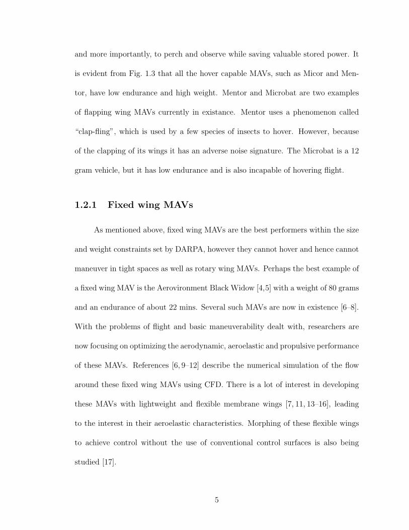
1.2.1 Fixed wing MAVs

As mentioned above, fixed wing MAVs are the best performers within the size

and weight constraints set by DARPA, however they cannot hover and hence cannot

maneuver in tight spaces as well as rotary wing MAVs. Perhaps the best example of

a fixed wing MAV is the Aerovironment Black Widow [4,5] with a weight of 80 grams

and an endurance of about 22 mins. Several such MAVs are now in existence [6–8].

With the problems of flight and basic maneuverability dealt with, researchers are

now focusing on optimizing the aerodynamic, aeroelastic and propulsive performance

of these MAVs. References [6, 9–12] describe the numerical simulation of the flow

around these fixed wing MAVs using CFD. There is a lot of interest in developing

these MAVs with lightweight and flexible membrane wings [7, 11, 13–16], leading

to the interest in their aeroelastic characteristics. Morphing of these flexible wings

to achieve control without the use of conventional control surfaces is also being

studied [17].

5

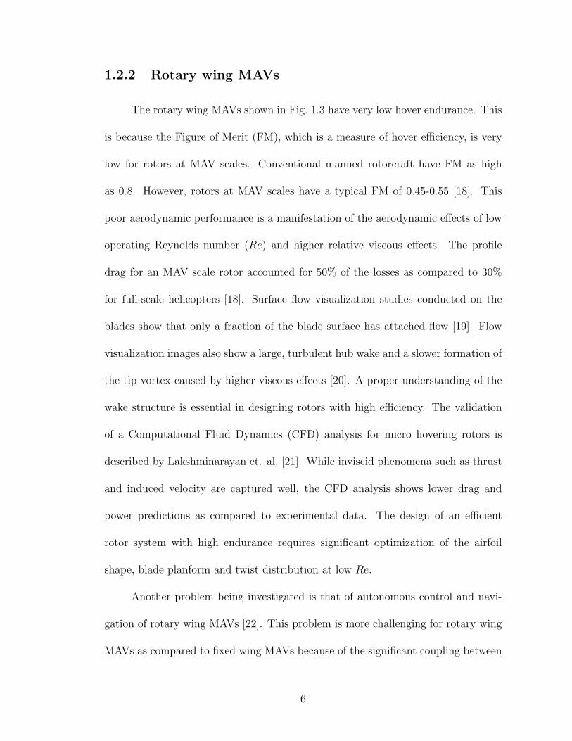
1.2.2 Rotary wing MAVs

The rotary wing MAVs shown in Fig. 1.3 have very low hover endurance. This

is because the Figure of Merit (FM), which is a measure of hover efficiency, is very

low for rotors at MAV scales. Conventional manned rotorcraft have FM as high

as 0.8. However, rotors at MAV scales have a typical FM of 0.45-0.55 [18]. This

poor aerodynamic performance is a manifestation of the aerodynamic effects of low

operating Reynolds number (Re) and higher relative viscous effects. The profile

drag for an MAV scale rotor accounted for 50% of the losses as compared to 30%

for full-scale helicopters [18]. Surface flow visualization studies conducted on the

blades show that only a fraction of the blade surface has attached flow [19]. Flow

visualization images also show a large, turbulent hub wake and a slower formation of

the tip vortex caused by higher viscous effects [20]. A proper understanding of the

wake structure is essential in designing rotors with high efficiency. The validation

of a Computational Fluid Dynamics (CFD) analysis for micro hovering rotors is

described by Lakshminarayan et. al. [21]. While inviscid phenomena such as thrust

and induced velocity are captured well, the CFD analysis shows lower drag and

power predictions as compared to experimental data. The design of an efficient

rotor system with high endurance requires significant optimization of the airfoil

shape, blade planform and twist distribution at low Re.

Another problem being investigated is that of autonomous control and navi-

gation of rotary wing MAVs [22]. This problem is more challenging for rotary wing

MAVs as compared to fixed wing MAVs because of the significant coupling between

6

lateral and longitudinal motions introduced by the rotor. Also, the measurement

and control system must be small and light enough to be viable for MAVs.

1.2.3 Flapping wing MAVs

Taking a cue from nature, wherein, flight at small scales is characterized by

flapping wings, researchers are trying to mimic the wing motions of birds and insects

to build flapping wing MAVs. With the introduction of a constantly accelerating and

decelerating wing, the aerodynamics of such vehicles is highly unsteady in addition to

the high relative viscous effects because of low Reynolds number. Ornithopters like

the Microbat have been built and flown successfully by both researchers and model

airplane enthusiasts. From a biological perspective, these ornithopters are more like

birds than insects. This is because of fundamental differences in wing kinematics

between insects and birds. Birds primarily utilize wing flapping for propulsion, while

lift is generated by a combination of forward speed and wing flapping. This is the

reason for the lack of hover capability of these ornithopters. The differences between

insect-like and bird-like flapping are discussed further in the next section. A hover

capable flapping wing MAV, based on insect wing kinematics, is yet to be designed

and tested.

1.3 Bio-inspired design

An argument is often made that nature has almost exclusively resorted to

flapping flight because organic materials are not conducive to rotary wing flight.

7

However, at MAV scales, the reverse argument can also be made that, because of a

lack of materials which can mimic biological muscles, rotary wing devices are easier

to build and fly. At MAV scales, it is not yet clear whether rotary or flapping

wings are more efficient. Thus, at the very least, flapping wing flight needs to be

thoroughly investigated to determine its viability for MAVs. Also, since nature

has had millions of years to optimize its designs through the process of natural

selection, it is important for MAV designers to understand the fundamental physics

of flapping flight. Pines and Bohorquez [23] discuss the technical challenges facing

future MAV development. Low Reynolds number aerodynamics, light-weight and

flexible adaptive wing structures and highly efficient propulsion and power systems

need to be investigated thoroughly to build the next generation of MAVs. In flapping

flight, a mechanism that can mimic insect wing kinematics is also a major hurdle

which requires newer materials such as Electroactive Polymers (EAP) for artificial

muscles [24].

1.3.1 Insect Flight vs Bird Flight

In nature, flight has evolved into two different forms – insect flight and bird

flight. While both these forms are based on flapping wings, there are important

differences among them. Most birds flap their wings in a vertical plane with small

changes in the pitch of the wings during a flapping cycle. Figure 1.4 shows a number

of seagulls in different modes of flight ranging from take-off to cruise flight. This

picture illustrates the range of motion of typical bird wings. Since birds are much

8

Figure 1.4: Seagulls in different modes of flight [25]

larger than insects, incorporating muscles, feathers and other moving parts into the

wings is easier. Birds can control the shape and even the span of their wings to

adapt to different flight modes. However, without large changes in pitch, this type

of flapping cannot generate sufficient vertical force to support the weight in the

absence of any forward speed. As a result, most birds cannot hover. However, the

insect world abounds with examples of hovering flight. These insects flap their wings

in a nearly horizontal plane, accompanied by large changes in wing pitch angle to

produce lift even in the absence of any forward velocity. Among insects, there exist

animals that are capable of taking off backwards, flying sideward, and landing upside

down. Moreover, birds like the hummingbird, which are capable of hovering, have

wing motions very similar to hover-capable insects. Thus, insect-based bio-inspired

flight may present a hover-capable and highly maneuverable solution for MAVs.

9

Even among insects, there exist significant differences between the kinemat-

ics of various species. For example butterflies have large wings, which are clapped

together without any change in pitch. A number of unsteady and nonlinear phe-

nomena have been used to explain the relatively high lift generated by insects.

Weis-Fogh’s [26] clap-fling hypothesis is one such lift generating mechanism, but

it is limited to a few species of insects such as butterflies and so does not explain

the flight of other species. The University of Toronto-SRI Mentor is based on this

type of clap-fling mechanism. However, in addition to being noisy, such wings may

fatigue easily. Also, the efficiency of such a mechanism is not known. Another flight

mechanism is the use of tandem wings, such as those found on dragonflies, which

are remarkably agile fliers. Infact, in insects like the housefly or the honeybee, the

hind wings have evolved into structures called the Halteres. These serve as tiny

gyroscopes helping these insects in stabilizing themselves. Kinematic measurements

of a large variety of insects have shown that this type of flapping, with a pair of

wings undergoing large amplitude flapping and pitching motion, seems to be more

prevalent in nature. Although there is tremendous variation in the wing kinematics

of such insects, the basic elements of the kinematics are as shown in Fig. 1.5.

The distinction between bird-like flapping, henceforth referred to as ornithop-

tic flapping, and insect-based, or hover-capable flapping, is also important for an-

other reason. Ornithoptic flapping requires a much simpler mechanism to replicate

in contrast to hover-capable flapping. This is because of the large pitch changes

required by hover-capable flapping, in addition to flapping in a single plane like

ornithoptic flapping. This distinction has important consequences when one looks

10

Net Force

StrokePlane

Downstroke

Upstroke

Wing Path

SectionWing

Figure 1.5: Insect wing kinematics.

at the available literature on flapping flight, wherein, ornithoptic flapping has been

studied experimentally to a much greater extent. Literature on hover-capable flap-

ping consists of a considerable amount of research by biologists on the wing kinemat-

ics and morphology of actual insects and birds [26–30]. For experimental studies,

the problems encountered in making a hover-capable mechanism have been circum-

vented by making large, slow-moving, dynamically scaled models to mimic insect

wing kinematics [31–34].

1.4 Flapping Flight Research

The flight of insects has intrigued scientists for some time because, at first

glance, their flight appears infeasible according to conventional linear, quasi-steady

aerodynamic theory. Research on flapping wing flight can be broadly categorized

11

into experimental studies and analytical studies.

1.4.1 Experimental studies

Experimental studies have been conducted on live animals or by using scaled-

up flapping models. Measurement of wing properties and structure can be obtained

using dead animals. However, measurement of wing kinematics and flow visualiza-

tion require the animal to fly in a particular flight state, hovering or forward flight.

Needless to say, inducing a fly or a moth to carry out a required task is a difficult

proposition.

1.4.1.1 Experiments on live animals

Measurements of wing kinematics have generally been carried out using a

system of high speed cameras to capture the free flight of an insect within an en-

closure [27]. Based on calibration grids, the motion of the wings can be deduced

from the images captured by the cameras, regardless of the position of the insect.

Willmott and Ellington [28] used high speed videography to determine the wing

kinematics of a hawkmoth in hover and forward flight. Lift and drag coefficients of

hawkmoth wings and bodies were also measured [35]. Wang et. al. [30] measured

the kinematics and, torsion and camber deformation of dragonfly wings in flight.

Liu [36] measured the wing shape and kinematics of level flying seagulls, cranes and

geese. The kinematics were deduced from video of the birds in level flight.

In order to qualitatively and quantitatively understand bird flight several flow

12

visualization and force measurement studies have been conducted on live birds.

Spedding et. al. [37] studied the vortex wakes behind a nightingale trained to

fly in a wind tunnel. Usherwood et. al. [38] embedded pressure transducers and

accelerometers in the wings of geese to study their take-off. Hedrick et. al. [39]

embedded accelerometers in the wings of cockatiels, which were trained to fly in

a wind tunnel. Wing kinematics were also measured using a high speed camera.

Usherwood et. al. [40] obtained pressure measurements from transducers embedded

in the wings of pigeons. However, embedding transducers in live insect wings appears

infeasible because of their extremely small sizes.

Several flow visualization studies have also been conducted on live insects.

Srygley and Thomas [41] trained Red Admiral butterflies to fly to and from artificial

flowers through a wind tunnel. Smoke-wire flow visualization was carried out to

obtain a qualitative image of the flow around the wings. A number of unconventional

lift generating mechanisms were reported, including leading edge vortices, rotational

circulation and the ‘clap-fling’ mechanism. Thomas et. al. [42] carried out flow

visualization studies on free-flying and tethered dragonflies. A leading edge vortex

of constant diameter, extending from wing-tip to wing-tip, was reported on the fore-

wing during free-flight, when the wings were in counterstroke i.e., the fore-wings were

leading the hind-wings by a phase angle of 180◦. In a high acceleration maneuver,

the wings beat in phase with each other with a leading edge vortex extending from

the fore-wing to the hind-wing. Bomphrey et. al. [43] conducted flow visualization

and force measurements on a tethered hawkmoth in a wind tunnel. The leading

edge vortex was found to extend from wing-tip to wing-tip over the insect thorax.

13

The measured upward force showed a peak near the end of the downstroke, when

the leading edge vortex was present on the wing.

Lehmann and Dickinson [44] carried out tests on tethered fruit-flies in which

the flight force production was modulated in response to vertically oscillating visual

patterns. When the thrust equaled body weight, the variations in stroke amplitude

and frequency were found to be respectively, 2.7◦ and 4.8 Hz around their mean

value. However, at peak thrust, the wing kinematics were found to be limited to a

unique value of stroke amplitude and frequency. This suggests the existence of an

optimum value of stroke amplitude and frequency for maximum thrust production.

Also, very small changes in these stroke parameters are utilized by fruit-flies to

vary their flight forces. Dillon and Dudley [45] studied vertical force production by

tethered bees over a wide range of body mass. Heavier bees were found to produce

lower thrust and operated at a lower flapping frequency, although the stroke angle

did not change with body mass.

A few studies have been conducted on the material properties and structure

of insect wings. Song et. al. [46] studied the dimensions and elastic properties of

the forewing of a Cicada. The Young’s moduli of the wing membranes and veins

were found to be 3.7 GPa and 1.9 GPa, respectively. These values are quite low as

compared to metals or composite materials. Combes and Daniel [47, 48] measured

the flexural stiffness of insect wings and found that the spanwise flexural stiffness

was 1-2 orders of magnitude higher than the chordwise flexural stiffness. A finite

element analysis showed that this variation was primarily because of the leading

edge veins.

14

Although these studies provide qualitative and quantitative insight into insect

and bird flight, researchers have looked at other means of studying animal flight

in a controlled laboratory environment. This is because of the difficulty involved

in conducting such experiments on insects and also because tethering an animal or

having sensor wires trail from it can alter the performance of the animal.

1.4.1.2 Model experiments

Researchers have studied large, slow-moving models in order to understand the

physics of flapping wing flight. Dickinson and Gotz [31] experimentally measured

the forces acting on a flat plate, translating and rotating in a sucrose solution at

a Reynolds number varying from 75 to 225. Such low Reynolds numbers are char-

acteristic of the Fruit Fly Drosophila Melanogaster. Their experiments showed the

transient forces acting on a wing which is accelerated from rest to a constant veloc-

ity. At high pitch angles, initial values of the lift coefficient were found to be higher

than the steady values. The flow pattern was also very unsteady at high pitch an-

gles, with an alternating pattern of leading and trailing edge vortices. Van den Berg

and Ellington [32] developed a model ’flapper’ using four d.c. servo motors and an

elaborate gearbox. This model could accurately mimic the wing motions of a Hawk-

moth. The wings were 46.5 cms long and were flapped at a frequency of 0.3 Hz in

order to match the operating Re to that of a real Hawkmoth. A leading edge smoke

rake was used to visualize the flow pattern. A leading edge vortex was observed

on the wing with a 3D structure, smaller towards the wing root and larger out-

15

board [33]. Recent experiments conducted on a dynamically scaled model (Robofly)

have shown that insects must take advantage of unsteady aerodynamic phenomena

to generate thrusts greater than those predicted by quasi-steady analyses [34]. Fig-

ure 1.5 shows the typical motion of an insect wing. This motion mainly consists of

four parts: a) downstroke, in which the wing translates with a fixed collective pitch

angle, b) near the end of the downstroke the wing supinates so that the blade angle

of attack is positive on the upstroke, c) upstroke and, d) pronation at the end of

the upstroke so that the angle of attack is positive on the downstroke. Figure 1.6 il-

lustrates the unsteady phenomena exploited by insects to generate and control high

lift. During the downstroke and upstroke (i.e. the translational phases) high lift

is produced because of a leading edge vortex on the wing. Supination and prona-

tion also produce significant lift from rotational circulation, which is also known as

Kramer effect. The third effect, wake capture, occurs as the wing passes through its

own wake, created during the previous half-stroke [34]. Sane [49] provides a review

of the aerodynamics of insect flight based on these experiments.

The Robofly experiments have shown that the leading edge vortex is the key

to explaining the high thrust generated by insects at low chord Reynolds numbers

(Re ∼ 150). At high Re, stable leading edge vortices have been observed on sharp

edge delta wings at high angles of attack. On these wings, the leading edge vortex

is stabilized by spanwise flow through the vortex core. Based on this analogy,

the presence of the attached leading edge vortex on the wing has sometimes been

explained by the presence of spanwise flow through the vortex core that transports

vorticity from inboard to outboard regions of the wing [50]. However, Birch et al. [51]

16

Leading Edge Vortex

Aerodynamic Force

Rotation

Wing Motion

Rotation

Starting Vortex

Wake From Previous Stroke

Wing Motion

Rotational Circulation

Wake Capture

Figure 1.6: Unsteady lift generating mechanisms in insects.

17

have shown that although spanwise flow does exist on the Robofly wings at an Re of

1,400, it is absent at a lower Re of 120. Ellington and Usherwood [50] also showed

that in rotary wing experiments conducted at Re from 10,000 to 50,000, the lift

coefficients at high Re dropped significantly as compared to lower Re, indicating a

weaker leading edge vortex at high Re. Recent flow visualization studies conducted

at a higher Re (∼ 15000) suggest that the vortex is not stable on the wing and that

multiple vortices may be generated during the stroke [52]. Thus, the effect of Re on

the leading edge vortex is not clearly understood. This is significant because of the

fact that flapping wing MAVs operate in the Reynolds number range 103 − 105.

In their experiments, Dickinson et. al. [34] decoupled the effects of wing trans-

lation and rotation, which could be predicted reasonably well using a quasi-steady

model. Using such a quasi-steady model, the effects of translation and rotation were

subtracted from the total measured force. The remaining forces were attributed to

wake capture caused by the interaction of the wing with its own wake. Birch and

Dickinson [53] also showed that a quasi-steady approximation of wake capture was

not accurate since this is a truly unsteady effect. Sane and Dickinson [54] carried

out a study on the effect of wing kinematics on thrust and drag. With short, sym-

metrical wing flips, the thrust was highest for a wing stroke of 180◦ and an angle

of attack of 50◦. Symmetrical flips were also found to produce high thrust and a

quasi-steady model predicted the time averaged thrust accurately although it did

not capture the time variation of vertical force. Maybury and Lehmann [55] studied

the interactions between scaled up dragonfly wings operating in a liquid medium.

Fore-wing performance was found to be unaffected by any changes in the phase

18

relationship between fore and hind-wing flapping. However, the hind-wing lift pro-

duction varied by a factor of two depending on the relative phasing of the flapping

cycles of the two wings. Lehmann et. al. [56] have also used such a model to study

the ‘clap-fling’ mechanism.

Based on the Robofly experiments, an ambitious project was started to build

a centimeter sized, 0.1 gram micro-robot called the Micro-mechanical Flying Insect

(MFI). Figure 1.7 shows a conceptual design of the MFI. The design target for the

MFI is the blowfly Calliphora, which has a mass of 100 mg, wing span of 11 mm and a

flapping frequency of 150 Hz [57]. Considerable amount of research has been done on

the wing actuation mechanism and a prototype MFI exists. The wing transmission

consists of two four-bar mechanisms, each actuated by a piezo unimorph, which

flap the wing in a horizontal stroke plane [58]. The four-bar mechanism magnifies

the relatively small amount of motion of the piezoelectric unimorph actuator to

flap the wing spar at a high stroke amplitude. These four-bars actuate the wing

root at two points along the chord. When the four-bars are actuated in phase,

the wing moves with a constant pitch angle. To change the wing pitch angle the

four-bars are actuated out of phase. Sitti et. al. [59] describe the development and

characterization of piezoelectric unimorph actuators for the MFI. A stroke amplitude

of 180◦ was achieved at 95 Hz frequency using a PZT-5H unimorph. Wood et. al. [60]

used composite materials to construct the MFI body achieving a high strength, low

mass structure that was easier to construct. Considerable amount of research has

focused on the design of a sensing and control system for the MFI [61–67]. These

studies focus on the development of bio-inspired sensors for the MFI using Ocelli for

19

Figure 1.7: Artists conception of the MFI (R.J. Wood).

insect like vision and Halteres for attitude sensing and control. However, all these

control studies rely on the Robofly measurements for the aerodyanmic characteristics

of such flapping wings. The use of such a simplified aerodynamic model to carry

out control system design is questionable. The Polyimide wings of the MFI weigh

0.5 mg. There are no available studies on the structural and aerodynamic design

of these wings. Flapping at such high frequencies, these light-weight, flexible wings

must deform considerably. Thus, aeroelastic design of the wings can improve their

aerodynamic efficiency.

Aeroelastic effects in ornithoptic or bird-like flapping have been studied ex-

perimentally to a much greater extent. Since the primary function of such flapping

wings is propulsion, these experiments tend to focus on the propulsive efficiency

of flapping airfoils. Shyy et.al. [25] provide a review of scaling laws, measurement

of wing kinematics of birds, low Re aerodynamics and flexible wing based flapping

20

flight. The effect of wing flexibility on ornithopter performance is quite well recog-

nized since all flying ornithopter models have very flexible wings. Ho et. al. [68]

studied the effect of wing spanwise stiffness on the lift generated by ornithoptic wings

in a free-stream flow. A computational fluid dynamics model coupled with an FEM

model was used to study the aeroelasticity of ornithoptic wings. Flexible membranes

were found to improve lift by minimizing the negative force peaks. Heathcote et.

al. [69] studied the effect of chordwise wing flexibility on the propulsive efficiency

of a wing undergoing pure heaving motion at zero freestream velocity. The thrust

to power ratio was found to be greater for the flexible wings as compared to a rigid

wing. Heathcote and Gursul [70] measured the thrust coefficient of plates of differ-

ent thicknesses, flapping at different frequencies, in freestream Reynolds numbers

from 0 to 27000, in a water tunnel. Again, some amount of flexibility was found to

be beneficial in generating thrust. Heathcote et. al. [71] studied the effect of span-

wise flexibility on thrust of a flapping wing. Some degree of spanwise flexibility was

found to be beneficial but, for a highly flexible wing, the tip displacement lagged the

flapping motion at the wing base, causing a loss of efficiency. Hong and Altman [72]

experimentally measured the lift force of a wing in pure flapping motion at zero free-

stream velocity. The generation of lift in the absence of any free-stream velocity was

attributed to span-wise flow. A non-planar wing with spanwise camber was found

to generate greater lift than a flat plate wing. Beasley and Chopra [73] also found

that a non-planar wing, with tip anhedral and a polynomial planform, performed

better than planar wings. Jones and Platzer [74] carried out an experimental and

numerical study on flapping wing propulsion. Several flapping configurations were

21

investigated including, a single airfoil flapping in a freestream velocity and two air-

foils in opposing plunge similar to ‘clap-fling’. Additional non-moving airfoils were

also placed downstream of the flapping airfoils to study interference effects. The

thrust was found to be maximum at zero flight speed. Jones et. al. [75] describe

the thrust measurements and flow visualization on a flapping wing MAV using two

airfoils in opposing plunge to generate thrust. The flexibility of the wing mount

was altered to investigate aeroelastic effects. Although the wing itself was quite

flexible, the flexible mount showed an increase in thrust upto a frequency of 20 Hz,

beyond which, a semi-rigid and rigid mount generated greater thrust. Jones and

Platzer [76] describe the development of their MAV based on this concept with a

maximum dimension of 23 cm and a mass of 11 grams. These studies clearly indicate

that aeroelastic design of flexible wings is very important for flapping flight.

1.4.2 Analyses

The development and validation of a comprehensive theory for unsteady force

generation by hover-capable flapping wings is partly hindered by a lack of exper-

imental data at the chord Reynolds numbers of interest (103 − 105). Most of the

analytical studies on the aerodynamics of flapping wings have examined rigid wings.

Some of these studies look at ornithoptic or bird-like flapping, i.e., flapping with-

out the pronation and supination phases of insect-like flapping. Some are restricted

to small disturbances while others are computationally intensive CFD simulations.

DeLaurier [77] developed an aerodynamic model for ornithoptic flapping, which has

22

been applied to the aeroelastic analysis of a large-scale ornithopter [78].

Analytical studies on the aerodynamics of hover-capable flapping may be clas-

sified as quasi-steady models, reduced order models, unsteady vortex lattice mod-

els and Computational Fluid Dynamics (CFD), in order of increasing complexity.

Quasi-steady analyses can be used to model the aerodynamics of flapping wings

provided experimentally measured lift and drag coefficients are used [79]. However,

these analyses do not account for unsteady effects such as the starting vortex or wake

capture [53]. Reduced order models utilize indicial functions to quantify the effects

of unsteady wing motion on airloads [80]. The unsteady vortex lattice method and

vortex particle methods have also been applied to flapping wing systems [81, 82].

Vest and Katz [83] used an unsteady vortex lattice model to study the aerodynam-

ics of bird flight. Eldredge [84] studied a 2-D wing undergoing large amplitude

flapping-pitching motion using a vortex particle method. The leading edge vortex

and starting vortex were observed from the resulting vorticity distribution.

CFD methods, which solve the incompressible form of the Navier-Stokes equa-

tions, are computationally intensive but they provide a clearer picture of the flow [85–

87]. Liu et. al. [88] carried out a CFD study of Hawkmoth wings undergoing both

flapping and rotational motions using an incompressible solver. Ramamurti and

Sandberg [86] used a finite element based flow solver to study the forces on a model

fruit-fly wing. The effect of phase difference between the flapping and rotational

motions was studied. High thrust was obtained when wing rotation occurred before

stroke reversal. Sun and Tang [89, 90] used CFD to predict the forces measured in

the Robofly experiments. Wu and Sun [91] used this analysis to study the effect of

23

Figure 1.8: Dragonfly wings.

various non-dimensional parameters such as Re, stroke amplitude and mid-stroke

angle of attack on the lift and drag coefficients. Sun and Wu [92] studied power

requirements in forward flight using this model. For comparison with experimental

data, these studies rely on model experiments conducted at very low frequencies.

For this reason, these analytical models do not account for aeroelastic effects caused

by wing bending and twisting under inertial and aerodynamic loading.

An important feature of insect wings is that they can elastically deform during

flight. Also, unlike birds or bats, insect muscles stop at the wing base so any active

control of the wing shape is not likely [93, 94]. Figure 1.8 shows the wings of a

dragonfly. These wings consist of veins covered with membranes, and are devoid of

any muscle. Passive aeroelastic design is therefore very important for insect wings.

The Robofly measurements are based on very low frequencies of motion because the

fluid used has a high viscosity. Thus wing bending and passive aeroelastic effects

24

are likely to be very small in the Robofly experiments.

1.5 Need for New Experimental Data

There are two major shortcomings of previous studies on insect-based, hover-

capable flapping wings. First, because of the mechanical complexity involved in

replicating the wing kinematics, these tests were conducted on scaled-up models in

a liquid medium. Thus the operating frequencies of these models is so low that

wing flexibility is not expected to play an important role. However, a practically

viable flapping wing MAV would require light-weight wings which would be quite

flexible. Second, the majority of such tests were conducted at low to very low Re

(100-1000). Based on their size, MAV Re’s lie between 104-105. Thus, there is a lack

of experimental data and testing in a Reynolds number range suitable for MAVs.

1.6 Need for Aeroelastic Modeling

With highly flexible wings operating at high frequencies, wing deformations

are expected to be quite significant. The effect of these deformations on wing per-

formance needs to be modeled and quantified. Experiments conducted on insect

wings suggest that their deformations are primarily caused by inertial forces, while

aerodynamic forces are an order of magnitude smaller and hence, they do not con-

tribute to the wing deformations [95]. If this is infact the case, it would be a double

edged sword, because, from a computational point of view, the wing structural and

25

aerodynamic analyses could be uncoupled. However, from an experimental point

of view, the small aerodynamic loads cannot be easily measured, especially in the

presence of large inertial forces.

Even though the aerodynamic forces may be small enough to neglect their ef-

fect on wing deformations, wing deformations will have an effect on the aerodynamic

loads. Thus it is important to have a complete aeroelastic model of the system.

Another point of concern is that the aeroelastic model must be computation-

ally efficient, if wing optimization studies are to be carried out. CFD studies are

computationally expensive and doubly so when coupled with a detailed computa-

tional structural dynamics model. Thus evaluating different wing designs is quite

difficult with such analyses.

1.7 Objectives and Approach

The objective of this research work is to measure the thrust generated by wings

mounted on a flapping-pitching mechanism, flapping at high frequencies in air. For

this objective, a force measurement methodology will be developed to measure the

inertial and aerodynamic forces acting on the flapping wing. Comparisons of the

measured thrust will be made with simple quasi-steady analyses. A more detailed

aeroelastic analysis will then be developed to understand the effects of wing elastic-

ity. As mentioned above, this aeroelastic model must be simple and computationally

efficient. A finite element model of the wing will be implemented and systematically

validated with experimental data. An unsteady aerodynamic model based on indi-

26

cial methods will be coupled with the structural model to predict the experimentally

measured thrust.

27

Chapter 2

Experimental Setup

In this chapter, the bio-inspired flapping wing mechanism used in this study

is described. Also, unique force and motion transducers which were mounted on

this mechanism are described. This setup was used to measure the thrust generated

by the flapping wing mechanism in the hover mode alongwith the flapping and

pitching motions at the wing base. A novel mechanism that utilizes the inertial and

aerodynamic forces acting on the wing, to produce a passive pitching motion, is also

described. Details of a flow visualization setup used as part of another study [52]

are also presented.

2.1 Bio-Inspired Flapping

Emulating the kinematics of insect or hummingbird wings at high frequencies

is a difficult proposition in terms of the mechanical complexity involved. This is

because, the required flap and pitch motions have large amplitudes. For example,

in insects, the flapping angle in the stroke plane may be as high as 160◦ with a pitch

change which is typically greater than 90◦. To achieve this type of wing kinematics,

28

with the flapping and pitching angles controlled separately, at least two actuation

systems must be used, one for flapping and another for pitching. Furthermore, the

pitch actuation mechanism must either be mounted on the flapping shaft or, it must

be able to actuate the pitch motion of the shaft through its large amplitude flapping.

A pitch actuator mounted on the flapping shaft would make the entire assembly too

heavy to flap at high frequencies. This is the reason why studies on insect-based

flapping wings have been conducted on models flapping in a liquid medium at very

low frequencies. In order to mimic insect wing kinematics a novel mechanism is

described by Tarascio and Chopra [3]. This bi-stable flapping mechanism is used in

the present work.

2.2 Bi-stable Flapping Wing Mechanism

The flapping wing test apparatus is a passive-pitch, bi-stable mechanism capa-

ble of emulating insect wing kinematics (Fig. 2.1). The desired flapping and pitching

motion is produced by a Hacker B20 26L brushless motor, which is controlled by a

Phoenix PHX-10 sensorless speed controller in combination with a GWS micropro-

cessor precision pulse generator. The motor shaft is rigidly attached to a rotating

disk, which in turn is attached to a pin that drives a scotch yoke. The scotch yoke

houses ball ends, which are attached to shafts that are free to flap with the mo-

tion of the yoke. As the shaft is actively flapped, pitch actuators, which are rigidly

attached to the shaft, make contact with Delrin ball ends at the end of each half-

stroke. This causes the shaft to pitch and, hence, generate the wing flip at the end

29

Figure 2.1: Flapping wing mechanism (Concept by M.J. Tarascio [3]).)

of the half-stroke.

The rotation of the shaft or “flip” at the end of each half stroke is generated

by the pitch assembly, which also serves to fix the pitch angle of the shaft during

the translational phases of the wing motion. The pitch assembly consists of the

main shaft, which is rigidly attached to a cam, and is, in turn, held in place by a

Delrin slider and a compression spring (Fig. 2.2). In combination with the pitch

stop, the entire assembly is bi-stable, in that it allows the shaft to rest in only two

positions. As the pitch actuator makes contact with the ball stops at the end of

each half-stroke, the cam is forced to rock over to the other stable position, with the

compression spring holding it in place until the next rotation. This pitch motion

30

Figure 2.2: Components of the pitch assembly.

is passive, being actuated by the flapping motion of the shaft. The pitch angle of

the wing during its translational phases is determined by the shape of the cam and

pitch stop shown in Fig. 2.2. Different pitch angles, such as 30◦ or 45◦, can be set

using different combinations of cams and pitch stops.

2.3 Thrust Measurement

Measurement of the flapping and pitching motions, and the small airloads

generated by a wing mounted on the flapping mechanism, poses a significant chal-

lenge. The flapping mechanism was initially designed to be mounted on the rotor

test stand at the Smart Structures Laboratory at the University of Maryland [3].

Figure 2.3 shows the flapping wing mechanism mounted on this test stand. The test

stand consisted of a 1000 gram load cell and a 25 oz-in reaction torque sensor to

measure the thrust and torque generated by the mechanism. The vertical force was

decoupled from the torque by using a spring-steel diaphragm which did not carry

any vertical load and passed only the moment to the torque sensor. A Hall effect

sensor mounted on the flapping mechanism, in combination with a magnet mounted

31

on the rotating disk, was used to determine the flapping frequency. However, tests

conducted using this test stand showed significant errors in thrust measurement.

Part of the problem was the very low thrust expected from a rectangular wing with

a small chord (1.5 cm). This was compounded by the fact that the mechanism itself

generated significant vibratory forces when flapping on the test stand. Keeping this

in view, it was decided to measure the forces acting on the wing directly at the wing

base. However, with this type of measurement, the pitch angle of the wing must

also be measured.

Commercially available sensors were found to be either too large or bulky to

be used on the flapping mechanism. Figure 2.4 shows some of these sensors. The

smallest available force sensors are thin beam load cells. However, these are generally

used for uniaxial measurements, whereas, a bi-axial measurement system was needed

because of the pitching of the shaft. The smallest potentiometers available for rotary

position measurement are too large to be mounted on the flapping shaft. For these

reasons, custom built transducers were used to measure the thrust generated by the

flapping wings.

2.3.1 Force Transducer

To measure the airloads, a load-cell was designed and built using Entran ESU-

025-500 piezoresistive strain gauges. These strain gauges are extremely small, with

a length of 1.27 mm and a width of 0.38 mm. The use of piezo-electric elements

makes them extremely sensitive, with typical gauge factors of 100 as compared to

32

Figure 2.3: Flapping wing mechanism mounted on the rotor test stand.

Bending beam load−cellsUniaxial

Precision rotary position sensor16 mm dia, 15 grams

(Midori America Corp.)(Transducer Techniques Inc.)

Figure 2.4: Commercially available sensors.

33

Figure 2.5: Load Cell.

conventional foil gauges which have typical gauge factors of 2. However, piezoresis-

tive gauges have a non-linear response at high strain values. Another disadvantage

is their high temperature sensitivity. Keeping these in mind, the load cell was de-

signed and tested to ensure that it operated within the linear range of the strain

gauges and temperature effects were minimized.

The load-cell was designed with a narrow beam cross-section (0.1′′ diameter)

on which two strain gauges were mounted to measure the loads in two orthogonal

directions (Fig. 2.5). Each strain gauge was connected in a half-bridge configuration

with a dummy gauge, which provided temperature compensation. The load-cell was

mounted at the end of the flapping shaft, with the wing being mounted at the end

of the load-cell.

The initial design of the load cell used a square beam cross-section because it

was easier to mount the gauges on a flat surface. Placing, mounting and aligning

the miniature gauges by hand was a challenge in itself. Because of gauge alignment

34

error, the square cross section load cell was found to be unsuitable for testing. This

was because, if the gauge was off-center, it introduced couplings between the two

orthogonal axes of measurement. Figure 2.6 shows the stresses on square and circular

cross-sections with a load at 45◦ to the horizontal. The strain gauge will show the

correct strain only if it is placed accurately at the center of a side of the square.

This was difficult to achieve. To minimize this error, a circular cross section was

used. On this cross-section, the mid-line of the U-shaped gauges could be aligned

with lines marked at 90◦ intervals on the surface. However, with this cross-section,

the gauges did not have a flat surface to bond with. This reduced the useful life of

the load cell.

Because strain gauges were used on the load-cell, only the moment acting at

the base of the wing was measured. To convert this moment into an equivalent

force, the distance from the wing base at which this force acts must be known. The

resultant aerodynamic force on the flapping wings was assumed to act at the point

defined by the second moment of wing area [27]. This distance, r2, was used to

determine the forces acting on the wing from the measured moments. These forces

were then transformed into vertical and horizontal components using the measured

pitch angle. The mean aerodynamic thrust was calculated by taking the ensemble

average of the vertical force over a number of flapping cycles.

35

’

(stresses not to scale)

−σ

+σ’

M

M −σ

+σ

−σ

+σ−2σ

+2σ

Load

M

M

2.54 mm

2.54 mm

2.54 mm

Strain gauge

Load

Figure 2.6: Stresses for square and circular cross-sections with a 45◦ load.

36

2.4 Motion Transducers

The load-cell measured the forces normal and tangential to the wing chord. To

obtain the vertical and horizontal components of these forces, the pitch angle of the

shaft was measured. This was done by using a Hall effect sensor in combination with

a semi-circular disk mounted on the shaft (Fig. 2.7). The disk had a tapered flexible

magnet in a semi-circular slot, with the Hall effect sensor mounted on the pitch

housing. The pitching motion of the shaft caused the magnet to move in relation to

the Hall effect sensor, producing a change in its output. A flexible magnet was used

because it could be easily cut to a taper and molded into the semi-circular slot on

the disk. In the first generation sensor, ten small magnets were arranged in a semi-

circle on the disk, which caused the Hall sensor output to change from its maximum

positive value to its maximum negative value every 18 degrees. This required careful

manual application of the calibration curve to convert the raw signal into the pitch

angle. However, with the tapered magnet, the calibration was simpler because of

the monotonic nature of the Hall sensor output.

In addition to a pitch motion sensor, another Hall sensor was used to measure

the flapping motion of the mechanism. In this case, another tapered magnet was

mounted on the cross-slide of the mechanism, with the Hall sensor fixed to the flap

bearing assembly, as shown in Fig. 2.8. Because the taper on the magnet was not

very smooth, the calibration was nonlinear for both the motion sensors. The flapping

motion was used to determine the flapping velocity, which, when multiplied with

the horizontal force on the wing, yielded the total aerodynamic and inertial power.

37

Figure 2.7: Pitch motion sensor.

Figure 2.8: Flap motion sensor.

38

When the flapping motion was differentiated to determine the flapping velocity, it

was passed through a low pass filter to eliminate the noise introduced by numerical

differentiation.

Two signal conditioning amplifiers (Vishay Measurements, Model 2311) were

used to excite the strain gauge circuits and also to amplify the output signal. The

Hall sensor outputs were amplified using an instrumentation amplifier (INA 128P).

These signals were interfaced with a computer using National Instrumentation (NI)

Data Acquisition (DAQ) hardware. The data were acquired using a GUI driven

Matlab program to simultaneously acquire and process the signals.

2.5 Passive Pitch Mechanism

A major concern with the bio-inspired mechanism described above was the

frequency that the wings could be tested at. This frequency was not only limited

because of the wing mass but also because of the pitch actuator hitting the ball

ends during the wing flip. Initial tests conducted on a pure flap mechanism with

the wing chord held vertical showed high thrust. This mechanism could be tested

at higher frequencies because there was no active pitching of the wing. Because of

this, the flapping wing mechanism was modified to include a torsion spring at the

base of the wing. This enabled passive pitching of the wing because of the inertial

and aerodynamic forces caused by the flapping motion. Figure 2.9 shows the details

of this mechanism. The flapping shaft passed through a set of bearings in the pitch

bearing assembly. This enabled the shaft to rotate to any angular position. This

39

Figure 2.9: Passive pitch mechanism.

rotation was prevented by a torsion spring made from a carbon fiber flexure, which

was held rigidly to the shaft. The rotation of the shaft caused the carbon fiber bar

to flex, thus providing the torsional stiffness. By moving the shaft-flexure connector

further inboard, the torsional stiffness could be increased.

2.6 Vacuum Chamber

Initial measurements conducted using the load cell showed that inertial forces

contributed significantly to the total measured load. In order to obtain the time

variation of airloads during a flapping cycle, the inertial forces had to be determined.

A vacuum chamber could provide an air free environment to measure these inertial

forces. An existing vacuum chamber, used for testing model rotors, was too large for

testing MAVs. Also, in this chamber, the flapping mechanism could not be observed

40

Figure 2.10: Vacuum Chamber

during testing. Because of this, a small vacuum chamber was designed and built

using clear acrylic material.

This vacuum chamber was designed and built using a 16′′ diameter, 1/2′′ thick

acrylic cylinder (Fig. 2.10). At the two ends of this cylinder, holes were drilled and

tapped for twelve 10-32 size screws equally spaced around the circumference. Two

acrylic plates were tightened on to the ends of the cylinder using these screws, with

a rubber gasket in between the end plate and the cylinder. Initial tests with a 0.4′′

thick acrylic plate showed excessive deformation of the end plate under external

41

pressure. An axisymmetric finite element analysis of the vacuum chamber was

carried out using IDEAS-FEM and 1′′ thick plates were found to be safe. Initial

testing with these thick plates showed that the vacuum chamber could achieve the

required vacuum safely and maintain it for at least one hour.

The upper plate of the chamber was fitted with a valve to connect to a vac-

uum pump. In addition, this plate also had a vacuum gauge and two electrical

feedthroughs for connecting the motor, force sensor and motion sensors. All vac-

uum chamber tests were conducted at a gauge pressure of 27′′ of mercury, which

corresponds to a 90% vacuum.

2.7 Flow Visualization

In order to qualitatively understand the unsteady aerodynamic mechanisms

involved, a flow visualization study was conducted [52]. The flow visualization

test stand consisted of a steel frame bolted to the ground, on which the flapping

wing mechanism was mounted approximately 4 ft. above ground level (Fig. 2.11).

Aluminum plates extended from ground level to approximately 3 ft. above the

mechanism to provide an image plane for the single wing. At the top of the aluminum

plates, an aluminum honeycomb extended 2 ft. horizontally. The seed for the flow

visualization was produced by vaporizing a mineral oil into a dense fog, which passed

through a series of ducts before reaching a diffuser mounted on top of the honeycomb.

The diffuser reduced the vertical velocity of the fog, while the honeycomb helped to

eliminate any swirl or turbulence in the flow. With the mechanism turned off, the

42

Figure 2.11: Flow visualization test setup.

smoke failed to reach the mechanism. This ensured that the velocity of the smoke

itself did not affect observed the flow patterns.

Flow visualization images were acquired by strobing the flow with a laser light

sheet generated by a dual Nd:YAG laser, as shown in Fig. 2.12. This laser was

triggered once every flapping cycle by a Hall effect switch mounted on the flapping

wing mechanism. Images were acquired using a Nikon D-70 6.1 megapixel digital

camera that was placed perpendicular to the laser light sheet as shown in Fig. 2.12.

43

Camera

Laser Sheet

Laser

Wing AxisFlapping

Figure 2.12: Flow visualization schematic.

To produce the seed particles, mineral oil was mixed with nitrogen under pressure

and then heated to its boiling point, where it became vaporized. As the vapor

emerged from the heat exchanger nozzle, it was mixed with ambient air, rapidly

cooled, and condensed into a fog.

44

Chapter 3

Experimental Results

The results of several experimental tests conducted on flapping wing systems

are described in this chapter. The following sections describe the thrust measure-

ments carried out on the bio-inspired flapping mechanism using different wings and

different stroke parameters. A quasi-steady analysis, implemented using empirical

lift and drag data from the Robofly measurements, was used to predict the thrust

generated by the wings. High frequency tests carried out on several lightweight

wings are also described. Thrust and power were also measured for a novel flapping

mechanism with passive pitching caused by aeroelastic forces.

3.1 Quasi-Steady Analysis

Experiments have shown that the lift and drag coefficients on flapping wings

are higher because of the leading edge vortex [34]. Previous quasi-steady analyses,

such as Ellington’s [27], did not account for this increased performance and hence

could not accurately predict the lift generating capacity of insect wings. However,

quasi-steady analyses can explain the lift produced by an insect wing if the effects of

45

Y

pX

fZ

fY

fX

iZ

i

p

Y

Z

p

Xi

θ

β

θ

β

Wing

Figure 3.1: Reference frames.

a leading edge vortex, on the lift and drag coefficients, are accounted for. This has

led to a revival of quasi-steady models in recent years [49]. However, such models

cannot account for the force peaks resulting from the induced inflow and wing wake

interactions because these effects are unsteady and three-dimensional in nature [53].

A blade element model similar to the one developed by Walker [79] was used to

predict the airloads on the flapping wings. In this analysis, the wing was assumed

to be rigid, i.e., the effects of elastic bending and torsion were ignored.

46

V (r,t)

θ

βdD(r,t)

dL(r,t)

V(r,t)

V (r,t)

α

n

x

Figure 3.2: Blade element.

The reference frames used to model the motion of the flapping wing are shown

in Fig. 3.1. The inertial reference frame XiYiZi has its origin at the center of

rotation. The flapping angle β denotes the rotation of the flapping reference frame

XfYfZf about the Zi axis as shown. The wing pitching reference frame XpYpZp is

obtained by rotating the flapping reference frame by the wing pitch angle θ, about

the Yf axis. It must be noted that the reference frames do not follow a right-handed

system. However, this allows the x-axis to be along the wing chord, in accordance

with thin-airfoil theory.

At a particular instant of time t, the forces parallel (dFx) and perpendicular

(dFn) to the wing chord, at a radial station r, are given by,

47

dFn(r, t) = dL(r, t) cosα+ dD(r, t) sinα (3.1)

dFx(r, t) = dL(r, t) sinα− dD(r, t) cosα (3.2)

where, dL(r, t) and dD(r, t) are the circulatory lift and drag which depend on the

angle of attack, α, as given by,

α = tan−1(vn(r, t)

vx(r, t)

)(3.3)

and where vx(r, t) and vn(r, t) are the velocities parallel and perpendicular to the

wing chord, respectively (Fig. 3.2). Based on thin airfoil theory, these velocities were

determined at the 3/4 chord location, which was found to give good agreement with

experimental results for the Robofly wings (for lift resulting from translation and

rotation). It must be noted that the velocities vx(r, t) and vn(r, t) were determined

based on kinematics alone, i.e., the induced inflow was not included in the analysis.

Although this is a serious shortcoming of the analysis, this model was found to give

good correlation with experiment [79]. The forces dFn and dFx were transformed

to the flapping reference frame through the pitch angle θ to determine the vertical

and horizontal circulatory forces.

Non-circulatory forces generated by the acceleration of the wing in a direction

perpendicular to the chord were calculated and added to the circulatory forces. The

non-circulatory force (dFnc), acting perpendicular to the wing chord, is given by,

dFnc =πρc(r)2

4vndr (3.4)

where, ρ is the density of the fluid, c(r) is the chord at radial station r, and vn is

the velocity normal to the wing chord, determined at the mid-chord location.

48

3.2 Hover Stand Tests

Initial tests were conducted on the hover test stand used for testing MAV

rotors. The wings used had a rectangular planform with 15 mm chord and 80

mm span [3]. These wings, cut from a titanium plate, were quite heavy. This

limited the maximum frequency that could be achieved on the flapping mechanism.

Figure 3.3 shows the thrust measured on the hover test stand using this wing.

Thrust prediction, made using the quasi-steady analysis, is also shown on this plot.

Although, the measurement error was quite large, it was surprising that the quasi-

steady analysis, with empirical lift and drag data, could at the very least, predict the

range of thrust expected from the wing. Three important conclusions were drawn

from this test.

1. The mass of the wing caused significant reduction in the frequency at which

the mechanism could be operated. With the solid titanium wing, the frequency

was limited to nearly 7.5 Hz.

2. The total thrust produced by the rectangular wing was too low to be measured

accurately on the hover test stand. The thrust predicted by the analysis was

also low.

3. The measurement errors were too large. This was mainly because of the large

vibratory loads on the test stand caused by the operation of the mechanism.

Infact, the data obtained from the load cell did not show any periodicity and

appeared to be white noise.

49

3 4 5 6 7 80

0.5

1

1.5

2

Frequency (Hz)

Thr

ust (

g)

Quasi−steady analysis

Experiment

o 15 mm

126 mm

80 mm

Figure 3.3: Thrust measured on the hover test stand for a rectangular wing.

50

Because of the large vibratory loads generated by the mechanism, it was de-

cided to measure the forces generated by the wing directly at the wing base. This

was accomplished using the load cell described in Chapter 2. Also, the wing plan-

form was modified by increasing the total wing surface area to increase the thrust

generated.

Wing planform

Based on the above observations, it was clear that, to achieve high thrust, the

wing must be light-weight and have a greater surface area than the rectangular wing.

The quasi-steady analysis also showed that a larger chord would increase thrust by

increasing the rotational circulation. The detailed structural and planform design of

a flapping wing was beyond the scope of the present work. Also, no guidelines were

in existence for the design of such wings. Figure 3.4 shows the wing planform chosen

along with a typical hummingbird wing. Comparison with a hummingbird wing was

made because hummingbirds are closest in terms of Reynolds number range to a

typical flapping wing MAV. The current wing planform retains the gradual taper of a

hummingbird’s wing, albeit with a larger chord towards the root, which may help in

generating higher thrust from rotational effects. Photographs of wing cross-sections

of insects do not show any well defined cross sectional shape [96]. For this reason,

a flat plate cross-section was used in the present study. However, during flapping,

the wing cross-sectional shape was dependent on the aeroelastic deformations of the

wing.

51

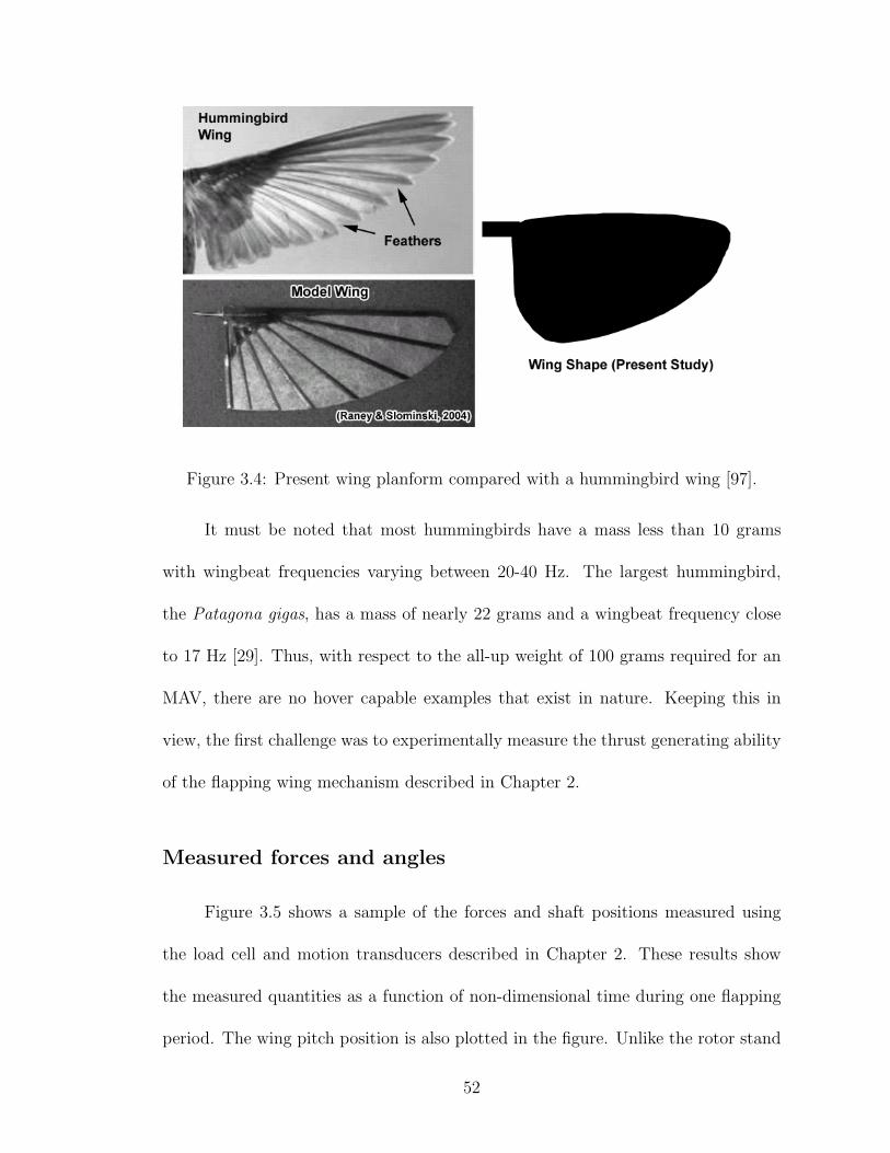
Figure 3.4: Present wing planform compared with a hummingbird wing [97].

It must be noted that most hummingbirds have a mass less than 10 grams

with wingbeat frequencies varying between 20-40 Hz. The largest hummingbird,

the Patagona gigas, has a mass of nearly 22 grams and a wingbeat frequency close

to 17 Hz [29]. Thus, with respect to the all-up weight of 100 grams required for an

MAV, there are no hover capable examples that exist in nature. Keeping this in

view, the first challenge was to experimentally measure the thrust generating ability

of the flapping wing mechanism described in Chapter 2.

Measured forces and angles

Figure 3.5 shows a sample of the forces and shaft positions measured using

the load cell and motion transducers described in Chapter 2. These results show

the measured quantities as a function of non-dimensional time during one flapping

period. The wing pitch position is also plotted in the figure. Unlike the rotor stand

52

0 0.1 0.2 0.3 0.4 0.5 0.6 0.7 0.8 0.9 1−200

−100

0

100

200

Thr

ust (

g)

0 0.1 0.2 0.3 0.4 0.5 0.6 0.7 0.8 0.9 1−50

0

50

β (d

eg.)

0 0.1 0.2 0.3 0.4 0.5 0.6 0.7 0.8 0.9 10

50

100

150

t/T

θ (d

eg.)

Freq. 9.07 Hz

Figure 3.5: Measured thrust, flapping angle and pitch angle during one flap cycle

at 9.07 Hz

measurements, the measurements carried out using the load cell showed periodic

force measurements, as expected. However, from the magnitude of thrust variation

during a flapping cycle, it was clear that inertial loads contributed significantly to

the total measured loads. This meant that the time variation of the airloads could

not be determined without recourse to vacuum chamber tests. However, the time

averaged vertical force must provide the aerodynamic thrust, since no thrust was

expected from the inertial forces.

Another concern with the bi-stable mechanism was the abrupt nature of the

53

pitching motion caused by the pitch actuator hitting the ball ends. Insects and

hummingbirds use biological muscles to accomplish such pitch changes in a smooth

manner. It is not known whether the type of pitching motion used in this study

would significantly effect the thrust generation capability of hover capable flapping

wings. However, Fig. 3.5 did not show any abrupt changes in the pitching motion of

the wing. It must be noted that the pitch angle was not fixed during the translational

motion of the wing, but varied by 10-15◦. This variation was caused by the flexibility

inherent in the pitch mechanism including the pitch stop and the spring loaded cam.

It was assumed that these factors would not significantly effect the thrust generation

capability of the mechanism. Furthermore, this working mechanism could fill a

serious gap in the availability of experimental data for hover capable flapping wings

at typical MAV Reynolds numbers.

3.3 Low Frequency Tests

Several tests were conducted at frequencies up to 10.5 Hz, with different wings

set at different pitch angles. In these tests, the first generation pitch motion sensor

was used and the flap motion was not measured. The following sections describe

the results of these tests. It may be noted that, the flapping mechanism used in the

present study was operated in air at frequencies as high as 12 Hz. The operating

Reynolds number based on the mean chord at a flapping frequency of 10 Hz was

approximately 17,000. This implies that the mean chord based Reynolds number

was higher than the transition Reynolds number of 10,000 for all frequencies higher

54

than approximately 5.8 Hz. Since the majority of tests in the present study were

conducted at frequencies higher than 5.8 Hz, the flow was not expected to be in the

transition regime.

Wings

The thrust generated by aluminum-mylar wings was measured for a number

of stroke and wing parameters. These wings, made from 0.508 mm thick aluminum

frames, are shown in Fig. 3.6. The only difference between Wings I and II was the

membrane material which made Wing II much lighter. It was found that Wings I and

II produced the same amount of thrust but Wing II could attain higher frequencies

on the flapping wing mechanism because of its lower mass. For this reason, results

are presented for Wings II and III only. All the results were based on a flapping

stroke angle of 80◦, i.e. the angle β varied from −40◦ to +40◦. Each wing was

tested at two pitch angles of 30o and 45o. A pitch angle of 30◦ implies that the

pitch was 30◦ during the downstroke and then changed to −30◦(150◦) during the

upstroke. Similarly for the 45◦ case, the pitch angle was 45◦ during the downstroke

and changed to −45◦(135◦) during the upstroke. Figure 3.7 shows the dimensions

of the wings and the root cut-out.

Load cell design

As described in Chapter 2, the initial design of the load cell used a square

cross-section because of the ease of mounting the miniature strain gauges on a flat

55

Figure 3.6: Scaled-up insect wings

56

������������������������������������������������������������������������������������������������������������������������������������������������������������������������������������������������������������������������������������������������������������������������������������������������������������������������������������������������������������������������������������������������������������������������������������������������

������������������������������������������������������������������������������������������������������������������������������������������������������������������������������������������������������������������������������������������������������������������������������������������������������������������������������������������������������������������������������������������������������������������������������������������������

148 mm

48 mm2.54 mm

55 mm

Mylar, 0.12 mm thick

5.08 mm

Aluminum frame, 0.508 mm thick

Figure 3.7: Schematic of planform showing root cut-out

3 4 5 6 7 8 9 10 110

0.5

1

1.5

2

2.5

3

Frequency (Hz)

Thr

ust (

gram

s)

Analysis (Wings I & II)

Experiment(Square load cell)

Experiment(Circularload cell)

Stroke : 80 o

Pitch : +30 o/−30o

Figure 3.8: Effect of change in load cell design on measured thrust

57

surface. This load cell had small cross-couplings between the two orthogonal axes

of measurement. Figure 3.8 shows the thrust generated by Wing II, when measured

with this square cross-section load cell. Also shown in the figure is the thrust

predicted using the quasi-steady blade element analysis. The thrust measured using

this load cell showed a higher-order variation as opposed to the quadratic variation

shown by the analysis. To check whether this discrepancy was caused by the cross-

coupling present in the load cell, a circular cross section load cell was designed and

built. On a square cross-section load cell, the strain gauges had to be mounted

with great precision if spurious surface strains were to be avoided. If the gauge

was off-center, it could pick up unwanted surface strains that caused the calibration

constants to change as the pitch angle of the load cell was varied. On a circular

cross-section, these spurious strains were minimized. Figure 3.8 shows the thrust

measured using this redesigned load cell. Although the discrepancy between the

analysis and experiment was still present, the circular load cell showed a quadratic

increase in thrust as the frequency increased. All remaining thrust measurements

were made using the circular cross-section load cell. Although this cross-section

provided good results, it suffered from the drawback that the strain gauges did

not have a flat surface to bond with. This led to a short useful life of these load

cells before the strain gauges had to be replaced, thus increasing the overall testing

time. It must be noted that, in Fig. 3.8, all the available data was plotted to show

the scatter in the data, and no error bars are shown. This was done because the

frequency that the mechanism operated at varied slightly for each test run.

58

3 4 5 6 7 8 9 10 110

1

2

3

4

5

6

Frequency (Hz)

Thr

ust (

gram

s)

Stroke : 80 o

Pitch : +30 o/−30o

Analysis (Wing III)

Analysis (Wing II)

Experiment (Wing II)

Experiment (Wing III)

Figure 3.9: Comparison of thrust generated by Wings II and III

Effect of pitching axis location

Figure 3.9 shows a comparison of the experimental measurements and analyt-

ical thrust predictions for the two wings at a pitch angle of 30◦. Wing III pitched

about the 20% chord location, compared to Wing II, which pitched about the 50%

chord location. This change in pitching axis increased the thrust produced by Wing

III because it produced more lift from rotational circulation during the pronation

and supination phases, as indicated by the analysis. It may be noted that even

though the analysis was quasi-steady, the thrust was not severely underpredicted

because of the experimental lift and drag data used in the analysis. The analysis

over predicted the thrust for Wing II. However, thrust prediction for Wing III was

quite good.

59

Effect of pitch angle

Figure 3.10 shows the thrust generated by Wing II at a pitch angle of 45◦ along

with the thrust generated at a pitch angle of 30◦. At a higher pitch angle, the thrust

was expected to increase. However, the experimental results show that the thrust

did not change when the pitch angle was increased for Wing II. The quasi-steady

analysis over-predicted the results, at both pitch angles, for Wing II.

Figure 3.11 shows the effect of change in pitch angle on the thrust generated

by Wing III. In this case, the experimentally measured thrust did show an increase

when the pitch angle was increased to 45◦. On the other hand, the predictions

did not show any significant change with pitch angle. This was because, when the

pitch angle for Wing III was increased, the total change in pitch was reduced. At

45◦ pitch angle, the wing flipped from 45◦ to 135◦, producing a total change of

90◦. However, when the pitch angle was 30◦, the total change in pitch was 120◦ as

the wing flipped from 30◦ to 150◦. The reduced flip angle at 45◦ pitch, reduced the

rotational circulation for Wing III. Because Wing III generated a significant amount

of lift from rotational circulation, the net increase in thrust was very small at 45◦

pitch angle.

Effect of pitch phase

Figure 3.12 shows the effect of a slight change in pitch phase on the thrust

generated by Wing III at a pitch angle of 45◦. To change the pitch phase, the ball

ends shown in Fig. 2.1 were moved slightly toward each other, thus causing the

60

3 4 5 6 7 8 9 10 110

1

2

3

4

5

6

Frequency (Hz)

Thr

ust (

gram

s)

Wing IIStroke : 80 o

Pitch : +30 o/−30o

and +45o/−45o

Analysis (45 o)

Analysis (30 o) Experiment (30 o)

Experiment (45 o)

Figure 3.10: Effect of wing pitch angle on thrust (Wing II)

3 4 5 6 7 8 9 10 110

1

2

3

4

5

6

Frequency (Hz)

Thr

ust (

gram

s)

Wing IIIStroke : 80 o

Pitch : +30 o/−30o

and +45o/−45o

Analysis (45 o)

Analysis (30 o)

Experiment (45 o)

Experiment (30 o)

Figure 3.11: Effect of wing pitch angle on thrust (Wing III)

61

3 4 5 6 7 8 9 10 110

1

2

3

4

5

6

Frequency (Hz)

Thr

ust (

gram

s)

Pitch: Baseline

Pitch: Early

Wing IIIStroke : 80 o

Pitch : +45 o/−45o

Figure 3.12: Effect of early rotation on thrust (Wing III)

pitch actuator to hit them early, producing an early pitch, (i.e. the wing flips over

earlier in the flapping cycle as compared to the baseline case). For this case, the

wing starts pitching 0.04T earlier than the pitch starting point for the baseline case,

where T is the time period of one flapping cycle. A delayed pitch case could not

be tested because of the limitations of the mechanism. Moving the ball ends away

from each other would lead to the pitch actuator hitting them late. However, in

this case, the wing flapping motion reversed direction before the pitching motion

was complete, i.e, before the wing had flipped over. Insects use changes in pitch

phase to change the lift generated by their wings. Figure 3.13 shows that the thrust

remains unchanged when Wing II pitches early. An interesting observation is the

nearly linear variation of thrust with frequency for the case of early pitching of

62

3 4 5 6 7 8 9 10 110

1

2

3

4

5

6

Frequency (Hz)

Thr

ust (

gram

s)

Wing IIStroke : 80 o

Pitch : +45 o/−45o

Pitch: Baseline

Pitch: Early

Figure 3.13: Effect of early rotation on thrust (Wing II)

Wing III (Fig. 3.12). The reduction in lift is unexpected since it has been reported

elsewhere [34] that early pitching may produce a positive wake capture, i.e., when

the wing flips early in the flapping cycle, its interaction with the wake created during

the previous cycle increases the total thrust. Figure 3.13 shows the effect of early

pitching on the thrust generated by Wing II. Although a limited amount of data

was available for this case, the thrust was nearly unchanged when compared to the

baseline case.

3.4 Vacuum Chamber Tests

Inertial forces constituted a large part of the total forces measured using the

load cell. To eliminate these inertial loads from the total measured loads, vacuum

63

0 −200

0

200Mean (Air) 2.4503

Mean (Vacuum)0.42508

Thr

ust (

gram

s)

0 0.1 0.2 0.3 0.4 0.5 0.6 0.7 0.8 0.9 10

100

200

Non−dimensional Time (t/T)

θ (d

egre

es)

−200

0

200Mean airload2.0253

Airl

oad

(gra

ms)

Vacuum

Air

Figure 3.14: Airloads obtained by subtracting inertial forces

chamber tests were conducted. When the wing was tested in vacuum, the frequency

attained by the mechanism was not the same as the frequency in air at the same

motor supply voltage. However, to subtract the inertial forces from the total loads,

the test frequencies in air and vacuum must match closely. This was achieved by

adjusting the motor supply voltage during the vacuum chamber tests to change the

frequency. Figure 3.14 shows the thrust generated in one flapping cycle by Wing II,

in air and in vacuum at a frequency close to 10.7 Hz. The frequency for the vacuum

test was 10.71 Hz, while the frequency in air was 10.65 Hz. Because these frequencies

were slightly different, the results were plotted against non-dimensional time in the

flapping cycle. Figure 3.14 also shows the airloads obtained after subtracting the

inertial forces from the total forces, and the pitch angle θ, measured both in air

and in vacuum. It is evident from this figure that the pitch angle varied slightly

64

3 4 5 6 7 8 9 10 11−1

0

1

2

3

4

5

6

Frequency (Hz)

Thr

ust (

gram

s)Wing IIStroke : 80 o

Pitch : +30 o/−30o

Air

Vacuum

Figure 3.15: Thrust measured in air and vacuum for Wing II

in vacuum because of a change in the dynamics of the drive mechanism. Also,

the temporal variation of airloads contained frequencies higher than the flapping

frequency, which may be caused by the elastic bending and twisting of the wing.

The variation in the airloads was expected to be an order of magnitude smaller than

the inertial loads. However, the results showed this variation to be of the same order

as the combined loads. This may be caused by the variation in the dynamics of the

mechanism itself. However, the average thrust measured in vacuum showed that, as

expected, Wing II generated a very small thrust at a pitch angle of 30◦ (Fig. 3.15).

The measurement error in the vacuum chamber data was larger as compared to the

measurement error in air. Although the vacuum chamber data did not provide a

reliable temporal variation of the airloads, it did increase the confidence level in the

65

thrust measurement methodology using the load-cell.

3.5 High Frequency Tests

Wing III

The low frequency tests were carried out to a maximum frequency of ∼10.5

Hz. In this section, results are presented for some high frequency tests carried out

on Wing III. The wing was tested at a pitch angle of 45◦ because the combination

of Wing III with 45◦ pitch was found to produce the maximum thrust in the low

frequency tests. Also, for these tests, the flap position was measured in order to

calculate the total inertial and aerodynamic power. Figure 3.16 shows the measured

thrust and power for Wing III up to a frequency of ∼11.6 Hz. The dashed lines

show curve fits through the data points. The thrust showed an increase up to a

frequency of 10.6 Hz, and then decreased sharply. The frequency range for which

these tests were carried out was very small because Wing III weighed 1.3 grams,

which required a lot of power input to the mechanism. It must be noted that the

power shown in Fig. 3.16 was computed from the measured stroke velocity and

the measured forces at the base of the wing. Therefore, this power includes the

aerodynamic and inertial power needed to move the wing at a particular frequency,

but does not give any information about the power required by the mechanism as

a whole. Without the wing, the mechanism could be run at almost 20 Hz. This

indicated that the mass of the wing was preventing the mechanism from moving at

66

high frequency. Also, only a limited amount of data could be acquired because, when

the frequency was increased further, the pitch stop (shown in Fig. 2.2) failed because

of the high forces. It must also be noted that, although the thrust dropped at high

frequency, the measured power showed a continuous increase as the frequency was

increased.

Light composite wings

Because of the large effect of wing mass on flapping frequency, several lightweight

wings were built with composite frames instead of aluminum. Figure 3.17 shows one

such wing with a carbon composite frame covered with a Mylar sheet. Table 3.1

shows the properties of these wings. All wings with a rectangular planform had the

same mean chord as Wings II and III. Wings IV, V and VI were covered with a

lightweight film called RC Microlite, which is similar to Monokote widely used by

model airplane enthusiasts. Wings VII and VIII used the same frames as Wings V

and VI, respectively, covered with a mylar sheet which is stronger and heavier than

RC Microlite. All the composite wings were made of rectangular planform because

it was easier to cut these shapes out. The first flap frequencies shown in Table 3.1

were determined from the impulse response of the wings, when mounted on the load

cell.

Figure 3.18 shows the measured thrust and power for Wings IV and V. The

thrust and power measured for Wing III are also shown on these plots. It is evident

from the range of frequencies for each wing that a lower wing mass helped in at-

67

9 9.5 10 10.5 11 11.5 121

2

3

4

5

6

7

Frequency (Hz)

Th

rust

(g

ram

s)

(a) Thrust

9 9.5 10 10.5 11 11.5 120.1

0.2

0.3

0.4

0.5

0.6

0.7

0.8

Frequency (Hz)

Po

wer

(W

atts

)

(b) Power

Figure 3.16: Thrust and power measured for Wing III at high frequency.

68

Wing Planform Pitching axis Frame Covering Mass (g) First flap

material material freq. (Hz)

II tapered 0.5c Aluminum Mylar 1.3 35.1

III tapered 0.2c Aluminum Mylar 1.3 36.1

IV rectangular 0.1c Carbon RC 0.49 24.4

composite Microlite

V rectangular 0.1c Carbon RC 0.65 34.9

composite Microlite

VI rectangular 0.1c Fiberglass RC 0.39 13.0

Microlite

VII rectangular 0.1c Carbon Mylar 0.86 34.2

composite

VIII rectangular 0.1c Fiberglass Mylar 0.61 -

IX tapered 0.2c Fiberglass mylar 0.58 15.03

X rectangular 0.1c Carbon mylar 0.68 -

composite

Table 3.1: Wing properties.

69

Carbon composite frame

Mylar skin

Figure 3.17: Wing VII.

taining high frequencies on the mechanism. The lower wing mass also led to lower

power as compared to Wing III. However, the thrust generated by Wings IV and V

was much lower than Wing III. Also, like Wing III, the thrust attained a maximum

value and then decreased with increasing frequency.

Figure 3.19 shows the thrust and power measured for Wings VI and VII. Again,

thrust and power for Wing III are also plotted for reference. Wing VI was the

lightest wing tested but it was also highly flexible. This is why the thrust generated

by this wing was very low. Wing VII was built to determine the effect of the skin

material on thrust. Wings IV and V used RC Microlite, which although lighter

than the Mylar sheet, had many wrinkles on it in addition to being very pliable. In

comparison, the Mylar sheet provided a relatively stiff, smooth membrane. Using

the Mylar instead of RC Microlite increased the thrust for Wing VII by a small

70

6 8 10 12 14 16−1

0

1

2

3

4

5

6

7

Frequency (Hz)

Thr

ust (

gram

s)

Wing IV

Wing V

Wing III

(a) Thrust

6 8 10 12 14 160

0.1

0.2

0.3

0.4

0.5

0.6

0.7

0.8

Frequency (Hz)

Po

wer

(W

atts

)

Wing III

Wing V

Wing IV

(b) Power

Figure 3.18: Thrust and power measured for lighter wings at high frequency.

71

6 8 10 12 14 16−1

0

1

2

3

4

5

6

7

Frequency (Hz)

Thr

ust (

gram

s)

Wing VI

Wing VII

Wing III

(a) Thrust

6 8 10 12 14 160

0.1

0.2

0.3

0.4

0.5

0.6

0.7

0.8

Frequency (Hz)

Po

wer

(W

atts

)

Wing III

Wing VII Wing VI

(b) Power

Figure 3.19: Thrust and power measured for lighter wings at high frequency

72

amount, although the frequency range was reduced because of the higher mass of

the Mylar sheet. A significant increase in the power was also noted. For both wings,

the thrust increased and then decreased with increasing frequency. Also, the scatter

in thrust measurements increased at high frequency for Wing IV and Wing VII.

3.6 Pure Flap Tests (Passive Pitch)

Frequency limitations of the mechanism did not allow the testing of heavier

wings at high frequencies. Part of this limitation stemmed from the large amount of

energy required to actively pitch the flapping shaft when the pitch actuator hit the

ball ends. To determine the thrust generated by the wings in a pure flapping motion,

the ball ends were removed so that there was no flipping of the shaft at the ends of

the stroke. However, there was some pitch flexibility in the mechanism because of

the spring loaded cam. For these tests, the wing was held on the shaft at a pitch

angle of 90◦. When the mechanism was turned on, the wing moved in a horizontal

stroke plane and pitched passively because of the inertial and aerodynamic forces

acting on the wing.

Figure 3.20 shows the thrust and power measured for Wings II, VII and VIII

at various flapping frequencies. Because the wing was held at 90◦ to the flow, like

a bluff body, the aerodynamic and inertial power was higher compared to the bio-

inspired flapping case. However, the surprising result was the thrust produced by

Wing VII, which was nearly 14 grams at a frequency of 19 Hz. Wing VIII could

generate nearly 5 grams of thrust, but Wing II produced very low thrust and also

73

6 8 10 12 14 16 18 20

0

5

10

15

Frequency (Hz)

Th

rust

(g

ram

s)

Wing VIII

Wing II

Wing VII

(a) Thrust

6 8 10 12 14 16 18 200

0.5

1

1.5

2

2.5

3

3.5

Frequency (Hz)

Po

wer

(W

atts

)

Wing VIII

Wing II

Wing VII

(b) Power

Figure 3.20: Thrust and power measured for pure flapping motion with passive

pitching of the wing.74

6 8 10 12 14 16 18 2070

80

90

100

110

120

130

Frequency (Hz)

Min

an

d M

ax p

itch

an

gle

Wing VIIIWing II

Wing VII

Wing VII

Wing VIII

Wing II

min

max

Figure 3.21: Minimum and maximum values of pitch variation.

required more power because of its higher mass. Figure 3.21 shows the minimum

and maximum values of the pitch angle variation for the three wings. The lower set

of dashed lines show curve fits through the minimum pitch angle values, while the

upper set show curve fits through the maximum pitch angle values. For Wing VII,

which produced the maximum thrust, the pitch angle changed from −10◦ to 20◦

about the 90◦ position, at the maximum frequency. Wings II and VIII generated

lower thrust with a smaller pitch angle variation. Based on these results, a passive

pitch mechanism was built, as described in Chapter 2.

75

3.7 Passive Pitch Mechanism

In this section, thrust and power measurements, made using the passive pitch

mechanism, are described. Figure 3.22 shows the measured thrust and power for two

positions of the shaft-flexure connector, one providing a stiff spring and the other

a soft spring. Wing VII was used for both tests. Figure 3.23 shows the minimum

and maximum values of the pitch angle variation for both cases. It is evident that

the soft torsion spring allowed a larger pitch variation and produced more thrust at

a slightly lower power than the stiff spring case. However, even with the spring in

the stiff position, the wing could generate approximately 9 grams of thrust with a

pitch variation of just ±10◦. This may be caused by the flexibility of the wing itself.

To achieve high frequency, and hence high thrust, the wing had to be made light

weight. However, a light wing also became very flexible. This made it very difficult

to separate the effect of the pitching of the shaft from the torsion of the wing caused

by its own flexibility.

Figure 3.24 shows the measured thrust and power for Wings III, VII and

X for various flapping frequencies. Figure 3.25 shows the corresponding values of

minimum and maximum pitch angle. The difference between Wing VII and Wing X

was that Wing X was machined rather than being cut with a blade like Wing VII.

Thus Wing X was lighter than Wing VII, and it could attain a higher frequency

on the flapping wing mechanism. However, at the same frequency, the pitch angle

variation for Wing X was smaller than Wing VII. This was reflected in the lower

thrust generated by Wing X as compared to Wing VII. The smaller pitch variation

76

4 8 12 16 200

2

4

6

8

10

12

14

16

18

Frequency (Hz)

Th

rust

(g

ram

s)

Stiff Spring

Soft Spring

(a) Thrust

4 8 12 16 200

0.5

1

1.5

2

2.5

3

3.5

4

Frequency (Hz)

Po

wer

(W

atts

)

Soft Spring

Stiff Spring

(b) Power

Figure 3.22: Thrust and power measured for passive pitch mechanism with stiff and

soft torsion spring for Wing VII.

77

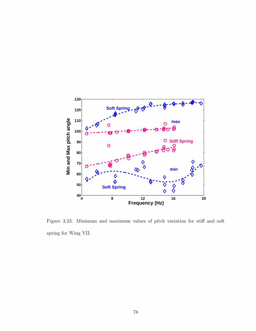
4 8 12 16 2040

50

60

70

80

90

100

110

120

130

Frequency (Hz)

Min

an

d M

ax p

itch

an

gle

Soft Spring

Stiff Spring

Soft Spring

min

max

Figure 3.23: Minimum and maximum values of pitch variation for stiff and soft

spring for Wing VII.

78

4 8 12 16 20 240

2

4

6

8

10

12

14

16

18

Frequency (Hz)

Th

rust

(g

ram

s)

Wing VII

Wing X

Wing III

(a) Thrust

4 8 12 16 20 240

0.5

1

1.5

2

2.5

3

3.5

4

Frequency (Hz)

Po

wer

(W

atts

)

Wing VII

Wing X Wing III

(b) Power

Figure 3.24: Thrust and power measured for passive pitch mechanism with various

wings.

79

4 8 12 16 20 2440

60

80

100

120

140

Min

an

d M

ax p

itch

an

gle

Frequency (Hz)

Wing VII

Wing III

Wing X

Figure 3.25: Minimum and maximum values of pitch variation for various wings

mounted on the passive pitch mechanism.

80

0 0.2 0.4 0.6 0.8 1−200

0

200

Thr

ust (

g)

0 0.2 0.4 0.6 0.8 1−50

0

50

Str

oke

(deg

.)

0 0.2 0.4 0.6 0.8 160

80

100

120

Non−dimensional time (t/T)

Pitc

h (d

eg.)

Figure 3.26: Time variation of loads and motion for Wing X at 22.3 Hz

for Wing X may be related to its lower mass and altered center of gravity location.

The location of the center of gravity behind the wing elastic axis is important to

generate a greater pitching motion because of the inertial forces acting on the wing.

Figure 3.26 shows the time variation of the thrust for Wing X, at high fre-

quency, during one flapping cycle along with the stroke position and shaft pitch

angle. The top figure also shows the mean thrust, and the pitch angle is plotted on

the bottom figure along with arrows showing the direction of motion of the wing.

The results are plotted against non-dimensional time in the flapping cycle. When

the wing motion was such that the pitch angle was less than 90◦ with respect to

the direction of motion, the thrust was positive. This was especially evident for

81

non-dimensional times between 0.7 and 0.9, where the thrust was nearly equal to its

mean value. It is also evident that the pitch angle variation was not in phase with

the flapping motion. This implies that with proper design and tuning of the torsion

spring it may be possible to further increase the thrust generated by the wings.

3.8 Flow Visualization

Detailed results of the flow visualization study conducted on the flapping wings

have been reported in Ref. 52. Flow features which are key to the aerodynamic

modeling of the flapping wings are described in this section. In the flow visualization

pictures, the laser sheet was at mid-span of the wing, and the camera was placed

perpendicular to the laser sheet, as shown in Fig. 2.12. The Reynolds number for

these tests was ∼15,000. Figure 3.27 shows a chordwise flow visualization picture

at mid-span, which clearly shows a leading edge vortex on the wing. The leading

edge vortex helps the wing generate thrust, even at the extremely high pitch angles,

without stalling. This is the first instance of a leading edge vortex being observed

on a flapping wing at Re ∼ 15, 000. Also, strobing the wing with the laser sheet

revealed the large amount of deformations that the wing was undergoing during

flapping.

Figure 3.28 shows a series of images acquired at different positions in the flap-

ping cycle starting from (b) the mid-point of supination to (l) the end of pronation.

Figure 3.28(c) shows the wing during supination. A number of vortical structures

were observed near the trailing edge during this rotational phase. As the wing

82

Figure 3.27: Flow visualization image showing the leading edge vortex.

started its translational motion, a powerful starting vortex formed and grew larger

throughout the downstroke (Fig. 3.28(d),(e),(f)). Figure 3.28(f) shows the wing at

the mid-point of the downstroke. One of the reasons for the high lift generating ca-

pability of insects, even at large pitch angles, is the presence of an attached leading

edge vortex on top of the wing. Such a leading edge vortex was observed on top of

the wing (Fig. 3.28(f)). Because of this vortex, the wing was able to generate thrust

even at a very high pitch angle. Figure 3.28(f)–(j) show the evolution of the leading

edge vortex during the latter half of the downstroke. Multiple leading edge vortices

were seen forming and shedding off the wing as shown in Fig. 3.28(h)–(j).

83

Figure 3.28: Flow visualization images acquired at different stroke positions (Ref. 52)

84

3.9 Summary

The thrust generated by wings, mounted on a flapping-pitching mechanism,

was measured for a number of wing and stroke parameters. The two wings tested had

the same planform shape. One wing pitched about the 50% chord location (Wing

II), while the other pitched about the 20% chord location (Wing III). The latter

produced more lift because of higher rotational circulation during the pronation

and supination phases. However, when the pitch angle of the wings was increased

from 30◦ to 45◦, the thrust produced by Wing III increased but the thrust for

Wing II remained the same. A slight change in pitch phase, so that pronation and

supination occur early in the flapping cycle, reduced the thrust produced by Wing

III. Again, the thrust produced by Wing II remained unchanged from the baseline

case.

The inertial forces produced by Wing II were measured by testing it in vacuum.

These forces were then subtracted from the total measured loads to obtain the

aerodynamic forces on the wings. Although the accuracy of the time varying airloads

obtained was questionable, the vacuum chamber tests showed nearly zero thrust

produced by the mechanism, as expected.

Wing III, which produced the maximum thrust, was also tested at higher

frequencies. However, the thrust showed a sudden drop at high frequency. The mass

of the wing significantly reduced the maximum frequency which could be attained

on the mechanism. Several light-weight composite wings were tested in order to

overcome this limitation of the mechanism. However, all these wings showed a drop

85

in thrust at high frequency. By measuring the stroke position of the wings, the total

aerodynamic and inertial power was computed at the base of the wing using the

measured loads. The effect of wing mass on power required was also evident from

the power curves.

Preliminary tests for a pure flapping motion with passive pitching of the shaft

because of the inertial and aerodynamic forces acting on the wing, showed significant

thrust generation by one of the wings tested. In this case the wing was held at a 90◦

angle and flapped in a horizontal plane. Because of the pitch flexibility of the shaft,

the inertial and aerodynamic forces caused the shaft to pitch in a passive manner.

To further explore the lift generation capability of a passive pitch flapping wing

mechanism, the bio-inspired flapping-pitching mechanism was modified to include a

torsion spring on the flapping shaft. The torsional stiffness of the spring could be

easily adjusted from a stiff condition to a soft one. When the spring was kept in the

soft position, the pitch variation was larger than the pitch variation for a stiff spring.

Also, the larger pitch variation for the soft spring helped generate greater thrust at

a slightly smaller power consumption than the stiff spring. The time variation of

thrust combined with the flapping and pitching motion of the shaft showed that the

pitching motion was not in phase with the flapping motion, leading to a reduction

in total thrust since the wing had an adverse angle of attack during part of the

flapping cycle.

The flow visualization images acquired, revealed the presence a leading edge

vortex on the wing. A large starting vortex was also observed. Multiple leading edge

vortices were noticed on the wing, with one vortex shedding towards the trailing

86

edge while another formed at the leading edge. An important observation from this

study was the large amount of wing deformations which were seen when the wing

was strobed using the laser light sheet.

87

Chapter 4

Aeroelastic Model

In this chapter the structural and aerodynamic analyses used to model the

aeroelastic behavior of hover-capable flapping wings are described. Since most in-

sect wings, and the wings used in experiments, are low aspect ratio wings, plate

finite elements were used to model these structures. The approaches available for

aerodynamic modeling range from indicial methods based on Wagner and Kuss-

ner functions to the computationally intensive Unsteady Vortex Lattice Method

(UVLM) and CFD analyses. In the present study, for coupling with the structural

model, an unsteady aerodynamic model based on indicial functions was used, since

this is the least complex and computationally efficient.

4.1 Structural Model

Figure 3.6 shows the aluminum-mylar wings used in the present study. A

beam model would not be adequate to represent such low aspect ratio wings. Beam

elements can only be used to model the aluminum frame, while plate elements must

be used to model the mylar. To avoid complications because of the use of dissimilar

88

elements, the entire wing structure was modeled using plate elements. However, the

use of plate elements introduces added complexity because a grid must be defined.

For rectangular wings, this would not be too difficult. However, with the irregular

planform of the wings, wing discretization becomes important.

4.1.1 Wing discretization

The process of discretizing the wing consists of defining nodes and elements on

the wing surface. This is usually accomplished by meshing the part to be modeled

using a structured or unstructured mesh. A structured mesh consists of a repeating

geometric and topological structure. Unstructured grids on the other hand have no

underlying structure. An important consideration in grid generation is the require-

ments of the finite element formulation. For example, certain quadrilateral plate

elements perform better if the elements are regular rectangles instead of quadrilat-

erals. Performance degrades if the opposing sides of the element are not parallel to

each other, i.e., if the element is not a rectangle. This is because, in the formula-

tion of these elements, the number of degrees of freedom do not allow the use of a

complete polynomial for interpolating the deformations within the element.

Based on the wing planform, an unstructured mesh would be most suited to

the current problem. However, available unstructured mesh generation algorithms

widely use triangular elements and not quadrilateral elements. The triangular el-

ements which were available did not perform as well as the rectangular elements.

Keeping in view the performance degradation of quadrilateral elements, a mesh us-

89

ing rectangular elements, with an irregular boundary, was chosen to discretize the

wing. To begin with, the wing domain was divided into a rectangular mesh as shown

in Fig. 4.1. The number of elements along each side of the rectangle could be varied

arbitrarily to refine the mesh. Based on the input wing geometry, the algorithm

accepted elements with at least a certain portion of their total area within the wing

domain, all other elements being rejected. The preprocessor then outputs ordered

sets of elements and nodes along with the element connectivity matrix.

4.1.2 Large overall motion

The structural model needs to account for the large overall motions of the wing,

which is discretized using plate finite elements, as shown in Fig. 4.2. The problem

of plates as well as arbitrary flexible bodies undergoing large overall motions has

been studied before [98–100], although, the method has not been applied to the

dynamics of flapping-pitching wings. In order to obtain accurate predictions of the

dynamics of a flexible body undergoing large overall motions, dynamic stiffening

must be accounted for in the formulation of the total kinetic energy. The equations

of motion were derived using Hamilton’s principle using the variation of the strain

energy and kinetic energy.

Strain Energy

Since the wings were quite thin, the effects of shear deformation were neglected.

Classical Laminated Plate Theory (CLPT) [101] was used so that the analysis would

90

Final Mesh

Initial Mesh

Elements kept/discarded basedon area within domain

Figure 4.1: Mesh generation

91

be applicable to both metals and composite materials. With the assumption of small

deformations, the linear strains for a plate can be written as,

εxx =∂u

∂x− z

∂2w

∂x2(4.1)

εyy =∂v

∂y− z

∂2w

∂y2(4.2)

γxy =∂u

∂y+∂v

∂x− 2z

∂2w

∂x∂y(4.3)

where, u, v and w are the deformations along the x, y and z directions, respectively.

In vector notation,

{ε} = {ε0}+ z{κ} (4.4)

where, {ε0} is the vector of membrane strains, {κ} is the vector of curvatures and

z is the coordinate perpendicular to the plane of the plate. Using the material

constitutive relation, σ = [Q]ε, the variation of strain energy can be written as,

δU =∫ ∫ ∫

V{δε}T [Q]{ε}dxdydz (4.5)

Substituting Eq. 4.4 in the above equation, and integrating across the thickness h,

the strain energy variation can be written as,

δU =∫ ∫

S({δε0}T [A]{ε0}+{δε0}T [B]{κ}+{δκ}T [B]{ε}0+{δκ}T [D]{κ})dxdy (4.6)

where, the matrices A, B and D are given by,

[A] =∫ h/2

−h/2[Q]dz (4.7)

[B] =∫ h/2

−h/2z[Q]dz (4.8)

[D] =∫ h/2

−h/2z2[Q]dz (4.9)

92

The matrix [B] represents the coupling between bending and extensional strains and

is zero for isotropic materials and also for composites with symmetric ply layup. It

must be noted that, as far as the analysis is concerned, the only difference between

an isotropic material or a composite is in the definition of the matrix [Q].

Kinetic Energy

Figure 4.2 shows the reference frames used to describe the overall motion of the

wing. The inertial reference frame Xi, Yi, Zi has its origin at the center of rotation.

The flapping angle β denotes the rotation of the flapping reference frame Xf , Yf , Zf

about the Zi axis as shown. The wing pitching reference frame Xp, Yp, Zp is obtained

by rotating the flapping reference frame by the wing pitch angle θ, about the Yf

axis. The relevant orthonormal transformation matrices are,

ip

jp

kp

=

cos θ 0 sin θ

0 1 0

− sin θ 0 cos θ

if

jf

kf

= [Tpf ]

if

jf

kf

(4.10)

if

jf

kf

=

cos β − sin β 0

sin β cos β 0

0 0 1

ii

ji

ki

= [Tfi]

ii

ji

ki

(4.11)

The position vector of a point on the wing in the pitching frame is given by

93

ZZi

Xf

Yf

a

β

a

θ

β

θ

ElementsWing Finite

pZ

pY

pX

f

Xi

Yi

Figure 4.2: Reference frames

94

(Ref. [98]),

~rp = {x1 + u−∫ x1

0

1

2

(∂w∂x

)2dx y1 + v −

∫ y1

0

1

2

(∂w∂y

)2dy w}

ip

jp

kp

(4.12)

The integral terms in the above equation represent the foreshortening effect in

the in-plane directions of the wing. These terms must be included to account for the

dynamic stiffening of the wing under centrifugal forces. Using the transformation

matrices described above, the position vector of a point on the wing can be written

in the inertial reference frame, as,

~ri = {x1 −∫ x1

0

1

2

(∂w∂x

)2dx y1 −

∫ y1

0

1

2

(∂w∂y

)2dy w}[Tpf ][Tfi]

ii

ji

ki

= ri1ii + ri2ji + ri3ki (4.13)

The components of the position vector are given by,

ri1 =

x1 + u−∫ x1

01/2

(∂

∂xw

)2

dx

cos θ cos β

+

y1 + v −∫ y1

01/2

(∂

∂yw

)2

dy

sin β

−w sin (θ (t)) cos β (4.14)

ri2 = −

x1 + u−∫ x1

01/2

(∂

∂xw

)2

dx

cos θ sin β

+

y1 + v −∫ y1

01/2

(∂

∂yw

)2

dy

cos β

+w sin θ sin β (4.15)

95

ri3 =

x1 + u−∫ x1

01/2

(∂

∂xw

)2

dx

sin θ + w cos θ (4.16)

In the above equations, the dependence of the deformations u, v and w on

(x, y, t) is implied. Also, the overall motions θ and β are functions of time t. The

velocity of a point on the wing can be found using the following equation,

~vi =d~ri

dt

= vi1ii + vi2ji + vi3ki (4.17)

The velocity components are given by,

vi1 =

(∂u

∂t−∫ x1

0

(∂w

∂x

)∂2w

∂t∂xdx

)cos θ cos β

−

x1 + u−∫ x1

0

1

2

(∂w

∂x

)2

dx

(

sin θdθ

dtcos β + cos θ sin β

dβ

dt

)

+

(∂v

∂t−∫ y1

0

(∂w

∂y

)∂2w

∂t∂ydy

)sin β

+

y1 + v −∫ y1

0

1

2

(∂w

∂y

)2

dy

cos βdβ

dt

−∂w∂t

sin θ cos β − w cos θdθ

dtcos β

+w sin θ sin βdβ

dt(4.18)

vi2 = −(∂u

∂t−∫ x1

0

(∂w

∂x

)∂2w

∂t∂xdx

)cos θ sin β

+

x1 + u−∫ x1

01/2

(∂w

∂x

)2

dx

sin θdθ

dtsin β

96

−

x1 + u−∫ x1

01/2

(∂w

∂x

)2

dx

cos θ cos βdβ

dt

+

(∂v

∂t−∫ y1

0

(∂w

∂y

)∂2w

∂t∂ydy

)cos β

−

y1 + v −∫ y1

01/2

(∂w

∂y

)2

dy

sin βdβ

dt

+∂w

∂tsin θ sin β + w cos θ

dθ

dtsin β

+w sin θ cos βdβ

dt(4.19)

vi3 =

(∂u

∂t−∫ x1

0

(∂w

∂x

)∂2w

∂t∂xdx

)sin θ

+

x1 + u−∫ x1

01/2

(∂w

∂x

)2

dx

cos θdθ

dt

+∂w

∂tcos θ − w sin θ

dθ

dt(4.20)

The variations of these velocity components are given by,

δvi1 =

(δ

(∂u

∂t

)−∫ x1

0

[δ

(∂w

∂x

)∂2w

∂t∂x+∂w

∂xδ

(∂2w

∂t∂x

)]dx

)

cos θ cos β −(δu−

∫ x1

0

∂w

∂xδ

(∂w

∂x

)dx

)sin θ

dθ

dt

cos β −(δu−

∫ x1

0

∂w

∂xδ

(∂w

∂x

)dx

)cos θ sin β

dβ

dt

+

(δ

(∂v

∂t

)−∫ y1

0

[δ

(∂w

∂y

)∂2w

∂t∂y+∂w

∂yδ

(∂2w

∂t∂y

)]dy

)sin β

+

(δv −

∫ y1

0

∂w

∂yδ

(∂w

∂y

)dy

)cos β

dβ

dt

−δ(∂w

∂t

)sin θ cos β − δw cos θ

dθ

dtcos β

+δw sin θ sin βdβ

dt(4.21)

δvi2 = −(δ

(∂u

∂t

)−∫ x1

0

[δ

(∂w

∂x

)∂2w

∂t∂x+∂w

∂xδ

(∂2w

∂t∂x

)]dx

)

97

cos θ sin β +

(δu−

∫ x1

0

∂w

∂xδ

(∂w

∂x

)dx

)sin θ

dθ

dtsin β

−(δu−

∫ x1

0

∂w

∂xδ

(∂w

∂x

)dx

)cos θ cos β

dβ

dt

+

(δ

(∂v

∂t

)−∫ y1

0

[δ

(∂w

∂y

)∂2w

∂t∂y+∂w

∂yδ

(∂2w

∂t∂y

)]dy

)cos β

−(δv −

∫ y1

0

∂w

∂yδ

(∂w

∂y

)dy

)sin β

dβ

dt

+δ

(∂w

∂t

)sin θ sin β + δw cos θ

dθ

dtsin β

+δw sin θ cos βdβ

dt(4.22)

δvi3 =

(δ

(∂u

∂t

)−∫ x1

0

[δ

(∂w

∂x

)∂2w

∂t∂x+∂w

∂xδ

(∂2w

∂t∂x

)]dx

)sin θ

+

(δu−

∫ x1

0

∂w

∂xδ

(∂w

∂x

)dx

)cos θ

dθ

dt+ δ

(∂w

∂t

)cos θ

−δw sin θdθ

dt(4.23)

The variation of the kinetic energy is then obtained from the following relation,

δT =∫ ∫ ∫

Vρ~vi · δ~vidxdydz (4.24)

where, ρ is the material density. Using Hamilton’s principle we have,

∫ t2

t1(δU − δT )dt = 0 (4.25)

Substituting Eqs. 4.6 and 4.24 in the above equation, we obtain the equations of

motion. Assuming the wing deformations u, v and w to be small, the higher order

non-linear terms may be neglected from the expansion of Eq. 4.24. The remaining

terms with orders of magnitude O(1) and O(ε) are given by,

98

∫ t2

t1δT 1dt =

∫ t2

t1

∫ ∫ ∫Vρ

([−(d2β

dt2

)y1 cos θ + cos2 θ

(dβ

dt

)2

x1

+

(dθ

dt

)2

x1

]δu +

[(dβ

dt

)2

y1 − 2 sin θ

(dθ

dt

)(dβ

dt

)x1

+ cos θ

(d2β

dt2

)x1

]δv +

[sin θ

(d2β

dt2

)y1 − cos θ(

dβ

dt

)2

x1 sin θ −(d2θ

dt2

)x1

]δw

)dxdydz dt (4.26)

∫ t2

t1δT εdt =

∫ t2

t1

∫ ∫ ∫Vρ

([−(d2β

dt2

)v cos θ − w sin θ

(dβ

dt

)2

cos θ

+2∂w

∂t

dθ

dt+

(dθ

dt

)2

u+ wd2θ

dt2+ cos2 θ

(dβ

dt

)2

u

−2

(dβ

dt

)∂v

∂tcos θ − ∂2u

∂t2

]δu +

[− ∂2v

∂t2+

(dβ

dt

)2

v

+2 cos θ∂u

∂t

dβ

dt− 2 sin θ

∂w

∂t

dβ

dt− w sin θ

d2β

dt2

+ cos θ

(d2β

dt2

)u− 2 sin θ

(dθ

dt

)dβ

dtu

−2w cos θ

(dθ

dt

)dβ

dt

]δv +

[− ∂2w

∂t2+ w

(dβ

dt

)2

−2

(dθ

dt

)∂u

∂t+ w

(dθ

dt

)2

−(d2θ

dt2

)u+ 2

∂v

∂tsin θ

dβ

dt

−w(dβ

dt

)2

cos2 θ − cos θ

(dβ

dt

)2

u sin θ

+ sin θ

(d2β

dt2

)v

]δw + x1 cos θ

(d2β

dt2

)∫ y1

0

∂w

∂yδ

(∂w

∂y

)dy

+ cos2 θ

(dβ

dt

)2

x1

∫ x1

0

∂w

∂xδ

(∂w

∂x

)dx−

y1

(d2β

dt2

)cos θ

∫ x1

0

∂w

∂xδ

(∂w

∂x

)dx

+

(dβ

dt

)2

y1

∫ y1

0

∂w

∂yδ

(∂w

∂y

)dy +

(dθ

dt

)2

x1

∫ x1

0

∂w

∂xδ

(∂w

∂x

)dx

−2 sin θ

(dθ

dt

)x1

(dβ

dt

)∫ y1

0

∂w

∂yδ

(∂w

∂y

)dy

)dxdydz dt (4.27)

99

It must be noted that, in the above equation, terms containing the variation

of velocities were eliminated by partially integrating them w.r.t time.

4.1.3 Finite Element Formulation

The expressions for strain and kinetic energy were discretized in space by

dividing the wing into finite elements. Figure 4.3 shows the degrees of freedom

(dof’s) of the plate element used. This element was first developed by Bogner, Fox

and Schmidt and is referred to as the BFS element [101]. It is one of the most

commonly used rectangular thin plate elements. The vector of elemental degrees of

freedom is given by,

{qe} =

{u1 u2 u3 u4 v1 v2 v3 v4 w1(∂w∂x

)1

(∂w∂y

)1

(∂2w∂x∂y

)1

w2

(∂w∂x

)2

(∂w∂y

)2

(∂2w∂x∂y

)2w3

(∂w∂x

)3(

∂w∂y

)3

(∂2w∂x∂y

)3

w4

(∂w∂x

)4

(∂w∂y

)4

(∂2w∂x∂y

)4}T

(4.28)

Within each element, the in-plane deformations u and v can be interpolated

using the element shape functions as,

ue(x, y, t) =4∑1

N1iui (4.29)

ve(x, y, t) =4∑1

N2ivi (4.30)

For the BFS element, the bending deformation w is expressed as,

we(x, y, t) = c0 + c1x+ c2y + c3x2 + c4xy + c5y

2 + c6x3 + c7x

2y + c8xy2

100

u

(d w/dxdy)vw

(dw/dx)1 1

2(dw/dy)

1

11 1

y

xz

u

(d w/dxdy)w

(dw/dx)2 2

2(dw/dy)

2

22 2

u

(d w/dxdy)w

(dw/dx)3 3

2(dw/dy)

3

33 3

u

(d w/dxdy)w

(dw/dx)4 4

2(dw/dy)

4

44 4v v

v

Figure 4.3: Element degrees of freedom

+c9y3 + c10x

3y + c11x2y2 + c12xy

3 + c13x3y2

+c14x2y3 + c15x

3y3 (4.31)

It must be noted that this polynomial is not complete. This is an issue with

most plate elements which require extra nodes and dof’s within the element to ob-

tain a complete polynomial. However, this element showed good convergence char-

acteristics for both static and dynamic problems. Substituting the 16 known nodal

deformations in Eq. 4.31, we obtain a set of equations for the unknown constants

ci, which can be solved to obtain the shape functions for the bending deformation.

The matrices N1, N2 and N3 are defined in Appendix A. In matrix form,

u

v

w

3×1

=

N1

N2

N3

3×24

{qe}24×1

= [N ]{qe} (4.32)

101

The 1× 24 vectors N1, N2 and N3 contain the shape functions for the u, v and

w deformations, respectively.

Strain displacement relation

The membrane strains and curvatures may be written as,

{ε0} =

∂∂x

0 0

0 ∂∂y

0

∂∂y

∂∂x

0

u

v

w

= [Γ1]{∆} (4.33)

{κ} =

0 0 − ∂2

∂x2

0 0 − ∂2

∂y2

0 0 −2 ∂2

∂x∂y

u

v

w

= [Γ2]{∆} (4.34)

where, [Γ1] and [Γ2] are operator matrices. Substituting Eq. 4.32 in the above

equations we get,

{ε0} = [Γ1][N ]{qe} = [H1]{qe} (4.35)

{κ} = [Γ2][N ]{qe} = [H2]{qe} (4.36)

The matrices [H1] and [H2] are functions of x and y within each element and,

relate the elemental deformations to the strain field within the element.

102

Static stiffness matrix

Substituting the above equations in Eq. 4.6, the elemental strain energy can

be written as,

δU e = {δqe}T

(∫ ∫e

[[H1]

T [A][H1] + [H1]T [B][H2] + [H2]

T [B][H1]

+[H2]T [D][H2]

]dxdy

){qe} (4.37)

where, the term within brackets defines the static stiffness matrix for one

element.

Ke =∫ ∫

e

[[H1]

T [A][H1]+[H1]T [B][H2]+[H2]

T [B][H1]+[H2]T [D][H2]

]dxdy

)(4.38)

Mass matrix and dynamic stiffness matrices

Using Eq. 4.32 the kinetic energy variation given by Eqs. 4.26 and 4.27 can be

written for a single element,

δT e = {δqe}T

(∫ ∫Aρt

[− (θ2 + β2 sin2 θ)[N3]

T [N3]{qe} − [N3]T [N3]{qe}

−(β2 sin θ cos θ + θ)x1[N3]T + sin θβy1[N3]

T + (sin θβθx1 − β2y1)[Hy]{qe}

+(sin θβθy1 − (cos2 θβ2 + θ2)x1)[Hx]{qe} − (θ + cos θ sin θβ2)

[N3]T [N1]{qe} − 2θ[N3]

T [N1]{qe}+ sin θβ[N3]T [N2]{qe}

+2 sin θβ[N3]T [N2]{qe}+ (θ − cos θ sin θβ2)[N1]

T [N3]{qe}

+2θ[N1]T [N3]{qe} − cos θβ[N1]

T [N2]{qe} − 2 cos θζ[N1]T [N2]{qe}

+(θ2 + β2 cos2 θ)[N1]T [N1]{qe} − [N1]

T [N1]{qe}+ (θ2 + β2 cos2 θ)x1[N1]T

103

− cos θβy1[N1]T − sin θβ[N2]

T [N3]{qe} − 2 sin θβ[N2]T [N3]{qe}

+β2[N2]T [N2]{qe} − [N2]

T [N2]{qe}+ (cos θβ − 2 sin θθβ)[N2]T [N1]{qe}

+2 cos θβ[N2]T [N1]{qe}+ (cos θβ − 2 sin θθβ)x1[N2]

T

+β2y1[N2]T

]dxdy

)(4.39)

where, the matrices [Hx] and [Hy] represent dynamic stiffening because of foreshort-

ening, and are given by,

[Hx] =∫ x1

0[N3,x]

T [N3,x]dx (4.40)

[Hy] =∫ y1

0[N3,y]

T [N3,y]dy (4.41)

where, the subscripts x and y, denote differentiation w.r.t x and y, respectively.

From Eq. 4.39, the elemental mass matrix, dynamic stiffness matrix and the

elemental force vector may be identified.

[M e] =∫ ∫

eρt([N1]

T [N1] + [N2]T [N2] + [N3]

T [N3])dxdy (4.42)

[KeD] =

∫ ∫eρt((β2y1 − sin θβθx1)[Hy] + ((cos2 θβ2 + θ2)x1

− sin θβθy1)[Hx] + (θ2 + β2 sin2 θ)[N3]T [N3]− (θ2

+β2 cos2 θ)[N1]T [N1]− β2[N2]

T [N2])dxdy (4.43)

{F e} =∫ ∫

eρt(

sin θβy1[N3]T − (β2 sin θ cos θ + θ)x1[N3]

T

104

+(θ2 + β2 cos2 θx1[N1]T − cos θβy1[N1]

T + (cos θβ

−2 sin θθβ)x1[N2]T + β2y1[N2]

T)dxdy (4.44)

Using the element connectivity matrix, the elemental matrices and force vec-

tors were assembled to obtain the global mass matrix [M ], the global stiffness matrix

[K], the global dynamic stiffness matrix [KD(t)] and the global force vector [F ]. The

stiffness matrix is time dependent because of the dynamic stiffness matrix [KD(t)].

A cantilever boundary condition at the wing root was then applied to these matrices

by eliminating the dof’s corresponding to the fixed nodes.

Numerical integration: Gauss quadrature

The area integrals in the above equations were evaluated using two-dimensional

Gauss quadrature. The integral of a generic function f(x, y) can be approximated

as, ∫ ∫Af(x, y)dxdy ≈

m∑i=1

n∑j=1

f(ξia, ηjb)WiWj (4.45)

where, m and n denote the number of gauss quadrature points in the x and y

directions, respectively, and Wi and Wj denote the corresponding Gauss weights.

Figure 4.4 illustrates the five point Gauss quadrature used in the present study.

Table 4.1.3 gives the coordinates and weights of the points.

In order to compute the dynamic stiffening matrices [Hx] and [Hy], the follow-

ing integrals were determined in closed form for each element,

∫ x

−a[N3,x]

T [N3,x]dx

105

Points ξi, ηj Weights Wi, Wj

0.0000000000 0.5688888889

±0.5384693101 0.4786286705

±0.9061798459 0.2369268850

Table 4.1: 5 point Gauss quadrature points and weights.

ξ ia η jb

x

y

2b

2a

, )(

Figure 4.4: Gauss quadrature points (5×5)

106

∫ y

−b[N3,y]

T [N3,y]dy

These matrices are defined in Appendix A.

Equation of motion

Using the kinetic energy variation, along with the wing strain energy functional

and using Hamilton’s principle, the equations of motion for a plate undergoing large

flapping and pitching motions were obtained. The dynamic response of a static wing

is governed by the following equation,

[M ] ¨{q}+ [K]{q} = 0 (4.46)

The eigenvalues and eigenvectors of this system are denoted by Λ and Φ. When the

wing motion is prescribed, i.e. θ(t) and β(t) are known as a function of time, the

equations of motion can be written as,

[M ] ¨{q}+ ([K] + [KD(t)]){q} = {F (t)} (4.47)

where, the stiffness matrix is now a function of the prescribed overall base motions.

The modal matrix Φ for the static case was used to reduce the size of the above

system, by retaining the first ‘m’ modes in the analysis. All results were obtained

with the first five modes retained in the analysis. The nodal deformations can be

expressed in modal coordinates as,

{q} = [Φm]{q} (4.48)

107

where, [Φm] has m columns, with each column containing the eigenvector corre-

sponding to one mode. Substituting this equation in Eq. 4.47, the modal equations

can be obtained,

[Φm]T [M ][Φm]{¨q}+ [Φm]T ([K] + [KD(t)])[Φm]{q} = [Φm]T{F (t)} (4.49)

[M ]{¨q}+ [K(t)]{q} = {F (t)} (4.50)

Modal damping was included in the equations to account for the structural damping

of the wing. The resulting system of equations was integrated to obtain the motion

of the wing. Once the motion of the wing was known, the bending moment at the

base of the wing was obtained by a surface integral of the inertial loads acting on

the wing.

4.2 Aerodynamic Model

The aerodynamic analysis is a blade element formulation, based on the as-

sumption that the aerodynamic forces acting on a flapping-pitching wing can be

broken down into a number of components which are accounted for separately and

then added to obtain the total force. The effects of wing elastic deformations have

also been accounted for. The following components contribute to the total aerody-

namic force,

1. The translational and rotational circulation based on thin airfoil theory, with

wing elasticity effects included.

108

2. The effect of a leading edge vortex on the wing, determined by using Polhamus’

leading edge suction analogy for delta wings at high angles of attack [80,102,

103].

3. Non-circulatory forces based on thin airfoil theory [104].

4. The effect of the starting vortex on the translational and rotational circulation.

This was accounted for by using the Wagner function.

5. The effect of the shed wake and a tip vortex, accounted for by using the Kuss-

ner function. The induced inflow velocity was determined based on momentum

considerations.

Figure 4.5 shows the leading edge vortex and the structure of the wake at one radial

location along the wing. Figure 4.6 shows the flow velocities at this radial location.

In thin airfoil theory, the problem reduces to the determination of a circulation

distribution γ along the chord, as governed by the following integral equation,

1

2π

∫ c

0

γ(ξ)

(x− ξ)dξ = Vn + θ(x− ac)− w(x)− Vp

∂w

∂x(4.51)

It must be noted that, since the normal and parallel velocities were used in the above

equation, there was no small angle assumption involved. The velocities normal and

parallel to the wing chord are given by,

Vn = VH sin θ + Vv cos θ (4.52)

Vp = VH cos θ − Vv sin θ (4.53)

The circulation distribution γ can be determined by using the transformation ξ =

c/2(1− cosφ) and expressing γ(ξ) in terms of a Fourier series in φ [104],

109

Figure 4.5: Wake structure at one station along the span

θ

θ

w

Vn

Vp

Vh

Vv

ac

(x−ac)

Figure 4.6: Flow velocities

110

γ(φ) = 2V(A0

1 + cosφ

sinφ+

∞∑n=1

An sinnφ)

(4.54)

where, V is the total resultant velocity given by,

V =√V 2

H + V 2v (4.55)

Substituting eq. 4.54 in eq. 4.51, the Fourier series coefficients can be determined

as,

A0 =Vn

V+cθ

V

(1

2− a

)︸ ︷︷ ︸

Rigid

− 1

πV

∫ π

0wdφ− Vp

πV

∫ π

0

∂w

∂xdφ︸ ︷︷ ︸

Elastic

(4.56)

A1 =1

2

cθ

V︸ ︷︷ ︸Rigid

+2

πV

∫ π

0w cosφdφ− 2Vp

πV

∫ π

0

∂w

∂xcosφdφ︸ ︷︷ ︸

Elastic

(4.57)

An =2

πV

∫ π

0w cosnφdφ− 2Vp

πV

∫ π

0

∂w

∂xcosnφdφ︸ ︷︷ ︸

Elastic

(4.58)

The total circulation can be obtained by integrating γ(φ) along the chord,

Γ(t) = πV c(A0(t) +

A1(t)

2

)(4.59)

Thus the horizontal and vertical circulatory forces, without any unsteady effects,

can be determined as,

F cv (t) = ρVh(t)Γ(t) (4.60)

F ch(t) = ρVv(t)Γ(t) (4.61)

Elastic effects

In this section, the procedure to account for the elastic terms in eqs. 4.58 is

described. To illustrate this, consider the elastic part of the coefficient A0,

Ael0 = − 1

πV

∫ π

0wdφ− Vp

πV

∫ π

0

∂w

∂xdφ (4.62)

111

Let bp(x) be the vector of modal deflections for the pth structural mode at the cross-

section shown in Fig. 4.6. Similarly, let b′p(x) be the vector of modal slopes with

respect to x. The structural deformations across the chord at this station can then

be written as,

w(x, t) =Nm∑p=1

qp(t)bp(x) (4.63)

∂w

∂x(x, t) =

Nm∑p=1

qp(t)b′p(x) (4.64)

where, qp(t) represents the generalized coordinates and Nm is the number of struc-

tural modes retained in the analysis. Substituting the above equations into eq. 4.62

we get,

Ael0 = − 1

πV

Nm∑p=1

qp(t)Bp0 −

Vp

πV

Nm∑p=1

qp(t)B′p0 (4.65)

where, Bp0 and B

′p0 are given by,

Bpn =

∫ π

0bp(x) cosnφdφ (4.66)

B′pn =

∫ π

0b

′p(x) cosnφdφ (4.67)

with n = 0. Thus the dependence of the Fourier coefficients on the chordwise

deformation is accounted for by the aerodynamic coefficients Bpn and B

′pn , which can

be determined from the wing mode shapes a priori. Similarly, the other Fourier

coefficients can be written as,

A1 =2

πV

Nm∑p=1

qp(t)Bp1 −

2Vp

πV

Nm∑p=1

qp(t)B′p1 (4.68)

An =2

πV

Nm∑p=1

qp(t)Bpn −

2Vp

πV

Nm∑p=1

qp(t)B′pn (4.69)

112

Apparent Mass

For a flapping-pitching wing, the forces exerted by the fluid because of its ac-

celeration and deceleration must also be accounted for. Using the unsteady Bernoulli

equation, the pressure difference along the chord, caused by this added mass effect,

can be written as [104],

∆pnc =∂

∂t

∫ x

0γ(ξ, t)dξ =

∂

∂tΓ(x, t) (4.70)

Thus, the force normal to the wing caused by the added mass or non-circulatory

effect is,

F ncn = ρ

∫ c

0

∂

∂tΓ(x, t)dx =

ρc2

2

[32π∂

∂t(A0(t)V (t)) +

π

2

∂

∂t(A1(t)V (t))

π

4

∂

∂t(A2(t)V (t))

](4.71)

Substituting the expressions for the aerodynamic coefficients in the above

equation, the non-circulatory force can be obtained. The expression for F ncn is

provided in Appendix B. It may be noted that with the assumption of incompress-

ibility the non-circulatory forces act instantaneously at the moment of acceleration

or deceleration.

Leading Edge Suction

The suction force generated by the presence of a leading edge vortex on top

of the wing was modeled using an approach similar to that used for modeling the

vortices that occur on delta wings at high angles of attack [102, 105, 106]. This

method assumes that, at high angles of attack, the leading edge suction force on an

113

Fs

Fs

Fs

Leading edge suction

Attached Flow Over an Airfoil

Attached Flow Over a Sharp Edged Wing

Separated Flow Over a Sharp Edged Wing

Figure 4.7: Leading edge suction

airfoil is rotated by 90◦ and acts in the same way as the suction force that would

be generated by the presence of a vortex on top of the wing, as shown in Fig. 4.7.

The normal force is thus given by,

F poln (t) = ρΓ(t)Vh(t) sin θ (4.72)

where, Γ(t) is given by eq. 4.59.

114

Unsteady Effects

The effect of the starting vortex on the build up of circulation was accounted

for by using the Wagner function φw. Using this function, the effect of the starting

vortex on the forces given by eqs. 4.61, can be written using the Duhamel integral

as,

F cv (t) = ρVh(0)Γ(0)φw(t) + ρVh(t)

∫ t

0

dΓ

dσφw(t− σ)dσ (4.73)

F ch(t) = ρVv(0)Γ(0)φw(t) + ρVv(t)

∫ t

0

dΓ

dσφw(t− σ)dσ (4.74)

The expression for dΓ(t)/dt obtained from Eq. 4.59 is provided in Appendix B.

Garrick’s algebraic approximation to the Wagner function [107] was used in the

above equation,

φw(s) ≈ s+ 2

s+ 4(4.75)

where, s is the non-dimensional distance traveled by the airfoil in semi-chords. The

effect of the shed wake from the previous flapping strokes was accounted for by using

the Kussner gust response function ψk. The shed vorticity strength was computed

using the following equation,

γw(x, t) = − 1

V (t)

dΓ(t)

dt(4.76)

At the end of each stroke, this vorticity distribution was assumed to convect below

the wing by a distance viT2

, where, vi is the induced inflow velocity and T is the time

for one flapping cycle. With the vorticity distribution below the wing determined,

the gust velocity wg generated by this distribution can be found and used in a

115

Duhamel integral to determine its effect on the forces acting on the wing,

F kv = ρVh(t)

∫ t

0

dΓ

dwg

dwg

dσψk(t− σ)dσ (4.77)

F kh = ρVv(t)

∫ t

0

dΓ

dwg

dwg

dσψk(t− σ)dσ (4.78)

where, the Kussner function was approximated as,

ψ(s) =s2 + s

s2 + 2.82s+ 0.8(4.79)

A tip vortex was also modeled based on the assumption that all the vorticity beyond

the point of maximum circulation, along the wing span, rolls up into a tip vortex

(Ref. [107]). This tip vortex also convects downward based on the induced inflow

velocity and affects the gust velocity seen by the wing.

Induced Inflow Velocity

In order to determine the induced inflow velocity, vi, an iterative scheme was

employed. The total thrust produced by the flapping-pitching wing was computed

as the sum of all the above components. The inflow velocity was obtained from the

following equation which is based on momentum considerations,

vi =

√Ttotal

ρΦR2(4.80)

where, R is the total wing span and Φ is the wing stroke angle. The inflow was

assumed to be constant in space and time. The computation of forces and inflow

velocity was repeated until the inflow converged.

116

Chapter 5

Model Validation

The structural and aerodynamic models described in the previous chapter were

validated with data available in literature. The structural model was also validated

with experiments conducted on an aluminum plate undergoing pure flapping motion.

The aerodynamic model was validated with data available for the Robofly [34]. Since

these tests were conducted in oil at very low flapping frequencies, aeroelastic effects

were likely to be negligible. This makes these tests ideal for validating the rigid part

of the aerodynamic model.

5.1 Structural Model

5.1.1 Cantilevered plate spin-up

To validate the structural model, the spin-up motion of a cantilevered plate

was studied, as shown in Fig. 5.1. The rotational speed of the plate is given by,

ω =

ωs

(tts− 1

2πsin2πt

ts

)0 ≤ t ≤ ts

ωs t > ts

(5.1)

The geometric and material properties of the plate are,

117

l

b

t

ω

Figure 5.1: Rotating cantilever plate.

E = 70GPa, ρ = 3000Kg/m3, l = 1.0m,

b = 0.5m, t = 0.0025m, ν = 0.3

Figure 5.2 shows the tip deflection with respect to time and Fig. 5.3 shows the

RPM variation with time when ωs = 10 rad/s and ts = 5 s. The wing tip deflection

showed very good correlation with the results of Ref. 100, with and without dynamic

stiffening effects. The results also underscore the importance of including dynamic

stiffening effects to correctly model the response of the plate. Further results in this

study were obtained including dynamic stiffening in the analysis.

118

0 2 4 6 8 10−0.04

−0.03

−0.02

−0.01

0

0.01

Time (sec)

Tip

Def

lect

ion

(m)

Present Analysis

Jinyang &Jiazhen (2005)

Without dynamicstiffening

With dynamicstiffening

Figure 5.2: Tip deflection for spin-up motion of a rectangular plate.

0 2 4 6 8 100

10

20

30

40

50

60

70

80

90

100

Time (sec)

RP

M

Figure 5.3: RPM variation with time

119

5.1.2 Aluminum plate in pure flapping

The structural model was also validated experimentally for a rectangular alu-

minum plate undergoing pure flapping motion, as shown in Fig. 5.4. The geometric

and material properties of the plate were,

E = 70GPa, ρ = 2750Kg/m3, l = 0.089m,

b = 0.0381m, t = 5.08× 10−4m, ν = 0.3

In order to accurately predict the bending moment at the base of the wing, an

accurate measurement of the flapping acceleration was of prime importance. This

was because the bending moment was primarily dependent on the inertial forces

which in turn depend on the wing acceleration. With the flap position sensor de-

scribed in Chapter 2, only the flap position data was available. Numerical differen-

tiation of this data introduced large errors in the acceleration which, when given as

input to the analysis, caused large amplitude oscillations in the wing response. For

this reason, a miniature MEMS accelerometer (Fig. 5.5) was used to measure the

wing flap acceleration and a systematic validation of the analysis was carried out

using the test data. Figure 5.6 shows a comparison of the measured and predicted

bending moment at the base of the wing when the wing was moved arbitrarily at

a slow rate. Figure 5.7 shows the corresponding acceleration input to the analy-

sis. In this case, both the rigid and elastic analyses showed good agreement with

experimental data.

Figure 5.8 shows the measured flap acceleration when the plate was flapped

at a frequency of 2.7 Hz. With this acceleration input, a rigid analysis failed to

120

FlappingAxis

AluminumPlate

β

b

l

t

Figure 5.4: Aluminum plate in pure flapping motion.

Figure 5.5: MEMS accelerometer.

121

0 0.5 1 1.5 2−8

−6

−4

−2

0

2

4

6

8x 10

−3

Time (sec)

Ben

ding

Mom

ent (

N−

m)

ExperimentAnalysis(rigid)

Analysis(elastic)

Figure 5.6: Comparison of measured and predicted bending moment for a slow

support motion (flapping shaft shaken by hand).

0 0.5 1 1.5 2−250

−200

−150

−100

−50

0

50

100

150

200

Time (sec)

d2 β/

dt2 (

rad/

s2 )

Figure 5.7: Measured acceleration for slow support motion.

122

0 0.1 0.2 0.3 0.4 0.5 0.6 0.7−1500

−1000

−500

0

500

1000

Time (sec)

d2 β/

dt2 (

rad/

s2 )

Freq. 2.7 Hz

Figure 5.8: Measured acceleration at a flapping frequency of 2.7 Hz.

0 0.1 0.2 0.3 0.4 0.5 0.6 0.7−0.05

−0.04

−0.03

−0.02

−0.01

0

0.01

0.02

0.03

0.04

0.05

Time (sec)

Ben

ding

Mom

ent (

N−m

)

Analysis(rigid)

Experiment

Figure 5.9: Comparison of measured bending moment with a rigid analysis at 2.7

Hz.

123

0 0.1 0.2 0.3 0.4 0.5 0.6 0.7−0.05

−0.04

−0.03

−0.02

−0.01

0

0.01

0.02

0.03

0.04

0.05

Time (sec)

Ben

ding

Mom

ent (

N−m

)

Experiment

Analysis(elastic)

Figure 5.10: Comparison of measured bending moment with an elastic analysis at

2.7 Hz.

capture the measured bending moment variation, as shown in Fig. 5.9. On the

other hand, the elastic analysis captured the bending moment variation, especially

at the peaks, although, there was some residual oscillation which was not present in

the experimental data. This was caused by the error in the measured acceleration.

Since the linear acceleration was measured, it had to be divided by the distance of

the accelerometer from the flapping axis, in order to obtain the angular acceleration.

Since this distance was limited by constraints of the mechanism, it amplified any

measurement error in the linear acceleration. The validation of the structural model

for an aluminum-mylar wing undergoing combined flapping and pitching is described

in the next chapter.

124

5.2 Aerodynamic Model

To validate the aerodynamic model, results were compared with experimental

data for the Robofly [53]. In these experiments, the wing was flapped with a stroke of

160◦ and the flapping frequency was 0.168 Hz. The wing pitch angle was 45◦ during

both the upstroke and the downstroke. The wing rotation was advanced by 12% of

the stroke period with respect to stroke reversal. The forces were measured for four

flapping cycles, with the wing starting from rest in the first cycle. For validating

the aerodynamic analysis results were compared with the forces measured during

the fourth cycle, when the wake below the wing is expected to be well established.

Since the Robofly operates at very low frequencies, elastic deformations of its wings

were expected to be small. This made it ideal for validating the aerodynamic model

without any elastic effects.

5.2.1 Wing motion

The wing motions β(t) and θ(t) were defined using piecewise continuous func-

tions, as shown in Figs. 5.11 and 5.12. During each half-stroke, the wing accelerates,

then moves with constant velocity β0 and thereafter decelerates. The wing acceler-

ation and deceleration phases last for a time period of ∆t/2. During these phases

the flapping velocity is given by,

β = −β0 cos πt− ts∆t

(5.2)

where, ts is the time at the start of the acceleration or deceleration phase. This

equation can be integrated to obtain the angular position of the wing. When the

125

wing moves with constant velocity, its position in the stroke plane is given by,

β = β0(t− ts) (5.3)

During the acceleration and deceleration phases, the following integral may be used

to determine the wing position,

∫ τ2

τ1βdt =

β0∆t

π

[sin

π(ts − τ2)

∆t− sin

π(ts − τ1)

∆t

](5.4)

During the acceleration and deceleration phases, the wing acceleration is given by,

β =πζ0∆t

sinπ(t− ts)

∆t(5.5)

Since it is usually the stroke amplitude which is specified and not the maximum

stroke velocity, the maximum stroke velocity can be determined as,

β0 =β0(

2∆tπ

+ t0) (5.6)

where, β0 is the amplitude of motion in the stroke plane.

As shown in Fig. 5.12, the wing pitch velocity is zero for time t0, and then

varies according to the following equation for time ∆t,

θ =1

2θ0

(1− cos

2π(t− ts)

∆t

)(5.7)

where, θ0 is the maximum pitching velocity and ts is the time at which pitching is

initiated. The following integral can be used to determine the pitch of the wing at

a given instant of time,

∫ τ2

τ1θdt =

θ0

4π

[2π(τ2 − τ1) + ∆t

(sin

2π(ts − τ2)

∆t− sin

2π(ts − τ1)

∆t

)](5.8)

126

∆t∆t ∆tt0t0

β = β0β =

β

T T T

f(t)

t/T = 0.5 t/T = 1.0

UpstrokeDownstroke

2T 2T

t/T

Figure 5.11: Definition of flapping motion.

During the pitching phase, the wing pitching acceleration is given by,

θ =πθ0

∆tsin

2π(t− ts)

∆t(5.9)

The maximum pitching velocity can be determined from the pitch angles θup

and θdown during the upstroke and downstroke, respectively,

θ0 =2(θup − θdown)

∆t(5.10)

5.2.2 Comparison with Robofly data

Figure 5.13 shows the flap and pitch velocities prescribed in the experiment.

These were used as inputs to the present analysis. Figure 5.14 shows the total aero-

dynamic force predicted by the analysis as a function of time during the flapping

cycle. The dashed line represents experimental data from Ref. 53. The peak oc-

curring just before the end of the downstroke was caused by three effects, namely,

the translatory circulation, rotational circulation and the apparent mass effect. A

127

θ = 0

θ = g(t)

t 1∆t ∆t−t1t 0 t 0

θ

TT T T T

t/T

Downstroke Upstroke

Figure 5.12: Definition of pitching motion.

significant contribution came from the translatory circulation, even though the pitch

angle was much larger than 45◦ at this point. The reason for this lies in the ideal

translatory lift coefficient from eqs. 4.59 and 4.61. This coefficient is given by,

Cideall = 2π sinα (5.11)

Figure 5.15 shows this ideal Cl plotted against the experimental values re-

ported in Ref. 34. It is clear from this figure that, unlike the experimental Cl, the

ideal Cl does not show any stall as the pitch angle increases beyond 45◦. This leads

to the overprediction of thrust near the end of the downstroke and upstroke, as seen

in Fig. 5.14. To account for this, the aerodynamic model was modified by using

the experimental Cl and Cd values to determine the circulation generated by the

translational motion of the wing. Figure 5.16 shows the vertical force computed

using this modified model. It is evident that the model with experimental Cl can

predict the aerodynamic forces better than the model with ideal Cl.

128

PSfrag

t/T

Rota

tionalsp

eed

rad/s

Downstroke Upstroke

θ

β

0 0.2 0.4 0.6 0.8 1-2

-1

0

1

2

Figure 5.13: Input velocities for Robofly kinematics.

t/T

Ver

tica

lfo

rce

(N)

Experiment

Analysis

0 0.2 0.4 0.6 0.8 1-0.2

0

0.2

0.4

0.6

0.8

1

1.2

1.4

Figure 5.14: Total vertical force with ideal Cl

129

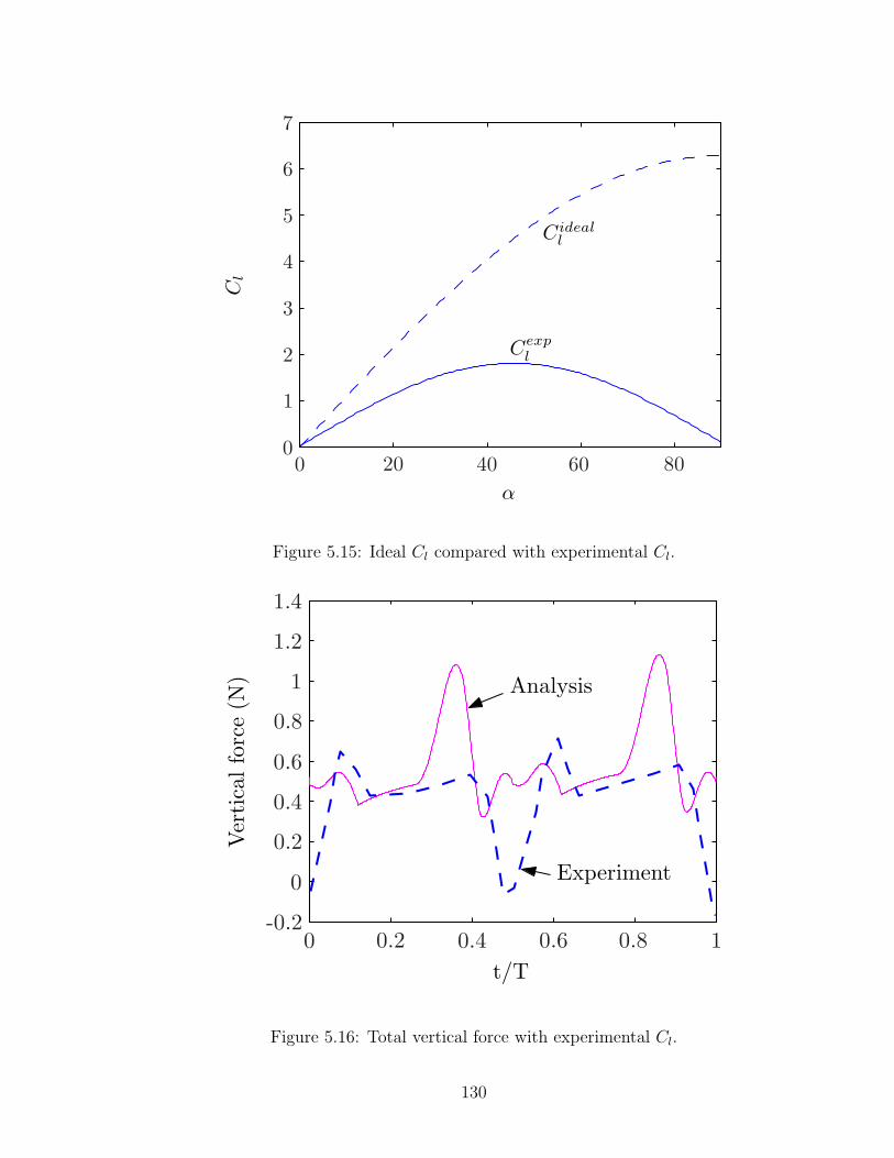
α

Cl

Cideall

Cexp

l

0 20 40 60 800

1

2

3

4

5

6

7

Figure 5.15: Ideal Cl compared with experimental Cl.

t/T

Ver

tica

lfo

rce

(N)

Experiment

Analysis

0 0.2 0.4 0.6 0.8 1-0.2

0

0.2

0.4

0.6

0.8

1

1.2

1.4

Figure 5.16: Total vertical force with experimental Cl.

130

Figure 5.17 shows the breakup of the total vertical force into its individual

components. There are several interesting features evident from this figure. First,

the force peak at the beginning of each half-stroke is because of non-circulatory

effects. Secondly, the slow rise in the force during the middle of each half stroke is

caused by a delayed build-up of circulation which is captured by the Wagner effect.

Thirdly, the leading edge vortex adds to the total thrust during the translatory part

of each half-stroke, although this effect is negated to some extent by the shed wake

from previous half-strokes, which is accounted for by the Kussner function. The

small peak in the circulatory force near the end of each half-stroke is caused by an

increase in rotational circulation. It is evident that the discrepancy between exper-

iment and analysis at the end of each half-stroke is caused by the non-circulatory

force. Figure 5.18 shows the comparison between experiment and analysis without

the non-circulatory effect. This shows an improvement in the agreement between

the analysis and experiment.

At this point, it is pertinent to mention that, in the experiments conducted on

the Robofly, the contribution of wing mass acceleration and gravity were removed

by using a dummy inertial wing (Ref. 34, pp.1960). What is unclear is the way

in which this subtraction of inertial effects, using a dummy inertial wing, effected

the non-circulatory forces measured on the real wing. Reference 34 states that the

experiments were repeated for a kinematic pattern with and without a flat stroke

plane as shown in Fig. 5.19. In both cases, the force peak at the beginning of the half

stroke was present. However, the authors use this fact to eliminate non-circulatory

forces as the cause of this force peak, by stating that, for a flat stroke plane, non-

131

0 0.2 0.4 0.6 0.8 1−0.2

0

0.2

0.4

0.6

0.8

1

1.2

1.4

t/T

Ver

tical

forc

e (N

)

Fvc F

vk F

vpol F

vnc

Fvc

Fvpol

Fvk

Fvnc

Figure 5.17: Components of the total vertical force. F cv - circulatory (with Wagner

effect), F polv - leading edge suction, F nc

v - non-circulatory, F kv - Kussner effect.

t/T

Ver

tica

lfo

rce

(N) F

cv + F

polv + F

kv

Experiment

0 0.2 0.4 0.6 0.8 1-0.2

0

0.2

0.4

0.6

0.8

1

1.2

1.4

Figure 5.18: Vertical force without non-circulatory effects

132

planeIdealized flat stroke

Fnc

Fnc

Fnc

Actual wing kinematics with some out of plane motion

Wing

n

h

v

motion

Figure 5.19: Actual and idealized stroke planes and the non-circulatory force

t/T

Hori

zonta

lForc

e(N

)

Analysis

Experiment

0 0.2 0.4 0.6 0.8 1-2

-1

0

1

2

Figure 5.20: Total horizontal force

133

circulatory forces cannot contaminate the measurement of the vertical force. This

is an erroneous assumption because the non-circulatory force acts perpendicular to

the wing, and thus, for a wing held at a large pitch angle, it would effect both the

horizontal and vertical forces. Based on this assumption, the force peak at the start

of each half-stroke has been entirely attributed to wake capture, with no contribution

from non-circulatory effects. However, our predictions indicate that this force peak

can be explained, at least in part, by the non-circulatory forces.

Figure 5.20 shows a comparison of the computed horizontal force (i.e. drag)

with the horizontal force measured on the Robofly. During the translatory phase of

the motion, the analysis agreed closely with experiment. However, the force peaks at

the beginning and end of each half-stroke were not captured very well. These peaks

were also caused by non-circulatory effects. Figure 5.16 shows an instantaneous rise

in the vertical force when the wing began its acceleration. Figure 5.20 shows that

the measured increase in drag, near the end of each half-stroke, was slower than

that predicted by the analysis. This indicated that compressibility effects may need

to be included in the the computation of the non-circulatory forces.

Figure 5.21 shows a comparison of the present analysis with that of Ref. [103],

along with the experimental data. It is evident from this figure that non-circulatory

forces also caused large errors in the analysis developed by Zbikowski et. al. The

difference between the present analysis and that of Ref. [103], lies in the derivation

of the non-circulatory forces. In Ref. [103], the non-circulatory forces were derived

for the entire wing using wing shape factors. However, in the present analysis,

the non-circulatory forces were determined from thin airfoil theory for each blade

134

0 0.2 0.4 0.6 0.8 1−1.5

−1

−0.5

0

0.5

1

1.5

t/T

Ver

tical

For

ce (

N)

Experiment

PresentAnalysis

Analysis(Zbikowski et.al.)

Figure 5.21: Vertical force compared with the analysis of Zbikowski et. al. [103]

element. Another observation from Fig. 5.21 is that the analysis of Ref. [103] does

not capture the slow rise in vertical force during the translatory part of the stroke,

which is captured by the present analysis. This slow rise in vertical force is a

manifestation of the starting vortex.

5.3 Summary

The structural model developed for a plate undergoing large overall motion

was validated with data available in literature and also with experiments conducted

on a rectangular aluminum plate in pure flapping motion. The input acceleration

provided to the analysis was a key factor in obtaining good correlation with exper-

imental data. However, currently available MEMS accelerometers measure linear

135

acceleration and not angular acceleration. Calculating the angular acceleration am-

plifies the measurement error in the linear acceleration.

A validation of the aerodynamic analysis was carried out by comparing the

analytical prediction of thrust with experimental data available in literature. These

experiments, conducted on wings moving at very low frequency in oil [34], are ideal

for validating the aerodynamic analysis without elastic effects. Some key observa-

tions of this validation study are summarized here,

1. The ideal translatory lift coefficient, obtained from thin airfoil theory was

inadequate to capture the aerodynamic forces. This is because, this coefficient

did not capture the lift stall shown by experimental data at angles of attack

greater than 45◦.

2. The predictions improved when the experimental lift and drag coefficients were

used in the analysis. However, there were discrepancies between the analysis

and experiment at the beginning and end of each half-stroke.

3. At the beginning of each half-stroke, a force peak was observed in the anal-

ysis. This peak was primarily caused by non-circulatory forces. This force

peak explained, at least in part, the force peak observed in the experiment.

However, in Ref. 34 this peak was attributed to wake capture alone, based on

the improper assumption that, for a flat stroke plane non-circulatory forces

could not affect the vertical force.

4. In Ref. 34, the forces caused by wing acceleration were removed by using a

dummy inertial wing. However, the effect of this subtraction, on the non-

136

circulatory forces, is unclear. With the non-circulatory forces removed from

the total thrust, the analysis showed a significant improvement in predicting

the measured thrust.

137

Chapter 6

Results

The thrust generated by a number of highly flexible and light-weight wings,

undergoing a bio-inspired flapping-pitching motion, was measured as reported in

Chapter 3. The high flexibility of these wings makes them ideal candidates for com-

parison with the analysis developed in this study. In this chapter, the aerodynamic

and structural analyses validated separately in the previous chapter were used to

predict the mean thrust measured on the bio-inspired flapping-pitching wings.

6.1 Wing Grids

Figures 6.1 and 6.2 show the finite element grids used to discretize two of

the light-weight wings tested on the bio-inspired mechanism. The frames of the

wing was made from aluminum. This frame was then covered with a light-weight

but sturdy mylar sheet. From an aerodynamic standpoint, Wing II and Wing III

were different because of the location of their pitching axes. This axis is defined

by the line xp = 0 in Figs. 6.1 and 6.2. Wing III pitched about its 20% chord

location while Wing II pitched about its 50% chord location. The following material

138

Radial distance (m)

Chord

wis

edis

tance

(m)

Mylar sheet

Aluminum framexp

yp

0.05 0.1 0.15

-0.06

-0.04

-0.02

0

0.02

0.04

Figure 6.1: Finite element grid for Wing III

properties were used for aluminum: Young’s modulus, E = 60 GPa, mass density,

ρ = 2400 Kg/m3, Poisson’s ratio, ν = 0.33 and thickness, t = 5.08× 10−4 m. The

material properties used for Mylar were: E = 7 GPa, ρ = 1250 Kg/m3, ν = 0.25

and t = 1.04× 10−4 m.

6.2 Bending moment comparison

The bending moment measured from a combined flapping-pitching motion of

Wings II and III was compared with the bending moment predicted by the analysis.

An important observation from our validation of the structural model was the need

for an accurate measurement of the flapping acceleration. This is because the accel-

erations directly effect the inertial loads acting on the wing, which, in turn, effect the

139

Radial distance (m)

Chord

wis

edis

tance

(m)

Mylar sheet

Aluminum framexp

yp

0.05 0.1 0.15

-0.06

-0.04

-0.02

0

0.02

0.04

Figure 6.2: Finite element grid for Wing II

measured bending moment. However, in the experiments conducted on the flapping

mechanism, only the pitch position was measured. For later tests, a flap position

sensor was also introduced. But the analysis required position, velocity and acceler-

ation, for the flapping and pitching motions, as inputs. Numerical differentiation of

the measured position introduced significant errors in the computed velocities and

accelerations. To alleviate this problem, a Fourier series was fit to the measured

flapping and pitch positions, as shown in Fig. 6.3. The coefficients of this Fourier

series were then used to determine the approximate velocity and acceleration. This

type of motion is henceforth referred to as approximated motion. Figure 6.4 shows

comparisons between the measured and predicted bending moments for Wing III at

various frequencies. These frequencies represent the higher range of all frequencies

140

0 0.2 0.4 0.6 0.8 1−50

0

50β

Experiment Fourier series fit

0 0.2 0.4 0.6 0.8 10

50

100

150

θ Experiment

Fourier series fit

0 0.2 0.4 0.6 0.8 1−40

−20

0

20

40

dβ/d

t

0 0.2 0.4 0.6 0.8 1−150

−100

−50

0

50

100

150

dθ/d

t

0 0.2 0.4 0.6 0.8 1−4000

−2000

0

2000

4000

t/T

d2 β/dt

2

0 0.2 0.4 0.6 0.8 1−2

−1

0

1

2x 10

4

t/T

d2 θ/dt

2

Flapping position Pitch Position

Flapping velocity Pitch velocity

Flapping acceleration Pitch acceleration

Figure 6.3: Position, velocity and acceleration used as inputs for the analysis

141

at which test data was available. The input motions for the analysis were approx-

imated from the measured flapping and pitch positions as described above. It can

be seen from this figure that, even with approximate flapping and pitching accel-

erations, the analysis could predict the bending moment satisfactorily at the lower

frequencies. At 10.96 Hz, there was some overprediction of the bending moment.

However, at 11.6 Hz, the analysis significantly overpredicted the bending moment.

Since a geometrically linear structural model was used, this may be part of the

reason for the overprediction. However, the approximation of the accelerations also

played a significant role. To illustrate this, the bending moment was recomputed

at a frequency of 11.6 Hz with a smooth motion used as an input to the analysis.

This smooth motion is compared with the approximated motion in Fig. 6.5. The

bending moment predicted by the analysis at a flapping frequency of 11.6 Hz, using

this smooth motion, is shown in Fig. 6.6. Although there was a significant error,

especially in phase, between the measured and predicted values, the peak to peak

variation showed significant improvement over the prediction using the approximate

motion. This underscores the need for an accurate measurement of the flapping

and pitching accelerations. The discrepancy in bending moment prediction at high

frequency is discussed further in a subsequent section.

6.3 Uncoupled Analysis

There is some experimental evidence to suggest that wing bending in hover-

ing insects is predominantly caused by inertial forces alone [108], with aerodynamic

142

0 0.1 0.2 0.3 0.4 0.5 0.6 0.7 0.8 0.9 1−0.05

0

0.05

ExperimentAnalysis

f=9.07 Hz

Ben

ding

Mom

ent (

N−

m)

0 0.1 0.2 0.3 0.4 0.5 0.6 0.7 0.8 0.9 1−0.1

−0.05

0

0.05

0.1

f=10.58 Hz

Ben

ding

Mom

ent (

N−

m)

0 0.1 0.2 0.3 0.4 0.5 0.6 0.7 0.8 0.9 1−0.1

−0.05

0

0.05

0.1

f=10.96 Hz

Ben

ding

Mom

ent (

N−

m)

0 0.1 0.2 0.3 0.4 0.5 0.6 0.7 0.8 0.9 1

−0.2

−0.1

0

0.1

0.2

f=11.6 Hz

t/T

Ben

ding

Mom

ent (

N−

m)

Figure 6.4: Bending moment variation compared with experimental data at various

flapping frequencies

143

t/T

β,θ

(deg

.)

Fourier series fit

Smooth motion

β

θ

0 0.2 0.4 0.6 0.8 1

0

50

100

150

Figure 6.5: Smooth motion vs Fourier series fit

t/T

Ben

din

gm

om

ent

(N-m

)

ExperimentAnalysis

f = 11.6 Hz

00 0.50.5 11-0.1 5

-0.1

-0.05

0

0.05

0.1

0.15

Figure 6.6: Comparison of analysis and experiment at 11.6 Hz with smooth motion

144

forces being an order of magnitude smaller than the inertial loads. Based on this

assumption, an uncoupled analysis was carried out. In this analysis, the wing defor-

mations were computed under inertial loading alone. These deformations were then

used in the aerodynamic analysis to determine the thrust generated by the wing.

6.3.1 High frequency tests (Wing III)

As discussed in Chapter 3, Wing III produced a maximum thrust of approx-

imately 6.5 grams at a frequency of 11 Hz and a pitch angle of 45◦. This was the

highest thrust generated among all the wings tested on the bio-inspired flapping-

pitching mechanism. However, this thrust dropped suddenly as the frequency was

increased to 11.6 Hz. For this reason, this wing was used to ascertain the predic-

tive capability of the present analysis. Figures 6.7 and 6.8 show the comparisons

between experiment and analysis for the high frequency tests conducted on Wing

III. These figures show results for both, a rigid wing and an elastic wing. Also, the

results were computed using both types of input motions for the analysis, i.e, the

approximated motion and the smooth motion.

It is evident from Fig. 6.7 that the approximated motion caused a significant

reduction in the thrust generated by the mechanism as compared to the smooth

motion. Also, the thrust predicted by the analysis using an approximated motion

agreed closely with the measured thrust, except at the highest frequency of 11.6 Hz.

Using the approximated motion, an elastic wing analysis showed close agreement

with the experimental results, although there was a slight overprediction of thrust

145

Frequency (Hz)

Thru

st(g

ram

s)

Rigid wing

Analysis (smooth motion)

Analysis (approximated motion)

Experiment

9 9.5 10 10.5 11 11.5 120

2

4

6

8

10

12

Figure 6.7: Rigid wing: predicted and measured thrust

Frequency (Hz)

Thru

st(g

ram

s)

Elastic wingAnalysis (smooth motion)

Analysis (approximated motion)

Experiment

no convergence

9 9.5 10 10.5 11 11.5 120

2

4

6

8

10

12

Figure 6.8: Elastic wing: predicted and measured thrust

146

Thru

st(g

ram

s)

Rigid Elastic Rigid Elastic

Approximated motion Smooth motion

︸ ︷︷ ︸ ︸ ︷︷ ︸

f = 10.96 Hz

Fcv F

polv F

kv

Fncv

-8

-6

-4

-2

0

2

4

6

8

Figure 6.9: Components of total thrust at 10.96 Hz (symbols: v-vertical, c-

circulatory, pol-Polhamus, k-Kussner, nc-non-circulatory)

at 10.96 Hz (Fig. 6.8). However, the most important result is that, for both the

elastic cases, the analysis showed a drop in thrust at a frequency of 11.6 Hz. For

these cases, the inflow did not converge because of the effect of the shed wake.

Figures 6.9 and 6.10 show the contribution of various components of the analy-

sis to the predicted thrust at the two highest frequencies. Figure 6.9 shows that wing

elastic deformations significantly increased the circulatory lift because of an increase

in the effective wing velocities. However, the large accelerations introduced by wing

elasticity, significantly reduced the non-circulatory contribution to the thrust. The

reason for a drop in wing thrust at 11.6 Hz can be understood from Fig. 6.10. For an

elastic wing, this figure shows the components after the first iteration only, since the

inflow did not converge. The non-circulatory forces introduced by wing elasticity

147

Thru

st(g

ram

s)

Rigid Elastic Rigid Elastic(after 1st

iteration)(after 1st

iteration)

Approximated motion Smooth motion︸ ︷︷ ︸ ︸ ︷︷ ︸

f = 11.6 Hz

Fcv F

polv F

kv

Fncv

-8

-6

-4

-2

0

2

4

6

8

Figure 6.10: Components of total thrust at 11.6 Hz

at this frequency, caused a significant reduction in the total thrust. This led to a

reduced inflow, which brought the shed wake closer to the wing plane. The vortic-

ity in the shed wake was quite strong because of the significant circulatory forces.

The close proximity of this vorticity to the wing plane was the primary cause for

non-convergence of the inflow.

6.3.2 Low frequency tests

Figure 6.11 shows a comparison between the analysis and experiment, for low

frequency tests carried out on Wing III at a pitch angle of 45◦. For reference, the

high frequency results are also shown in this figure. For the low frequency tests,

only the pitch motion was measured, hence, flapping position data was unavailable.

For these cases, the flap motion was assumed to be similar to the high frequency

148

Frequency (Hz)

Thru

st(g

ram

s)

Experiment

Analysis (rigid)

Analysis (rigid)

Analysis (elastic)

Analysis (elastic)

Wing pitch angle : 45◦

5 6 7 8 9 10 11 120

2

4

6

8

10

12

Figure 6.11: Comparison of experiment and analysis for Wing III at 45◦ pitch angle

tests. Figure 6.11 shows good agreement between experiment and analysis at low

frequencies, but there is some underprediction of thrust at the higher frequencies.

For these frequencies, an elastic analysis improved prediction. Figure 6.12 shows a

comparison between experiment and analysis for Wing III at a pitch angle of 30◦.

For this case, good agreement is seen with experimental data, for both rigid and

elastic analyses.

Figure 6.13 shows a comparison of experiment and analysis for the thrust

produced by Wing II at 30◦ and 45◦ pitch angles. This wing was characterized by

its pitching axis, which was located at the 50% chord location as compared to the

20% chord location for Wing III. For both pitch angles, the rigid analysis slightly

149

Frequency (Hz)

Thru

st(g

ram

s)

Experiment

Analysis (rigid)

Analysis (elastic)

Wing pitch angle : 30◦

5 6 7 8 9 10 11 120

2

4

6

8

10

12

Figure 6.12: Comparison of experiment and analysis for Wing III at 30◦ pitch angle

overpredicted the thrust. The elastic analysis also overpredicted the thrust at 30◦

pitch angle, but prediction improved at 45◦ pitch angle. However, an interesting

observation from these results is that, unlike Wing III, an increase in pitch angle

did not result in an increase in thrust. This effect was captured by the analysis. To

examine this closely, Fig. 6.14 shows the components of the total thrust, as predicted

by the analysis, at the two pitch angles. For the rigid case, the circulatory force

increased with the wing pitch angle, as expected. However, the non-circulatory force

reduced with an increase in pitch angle, keeping the total thrust nearly constant. For

the elastic case, both the circulatory and non-circulatory forces showed a reduction

with increasing pitch angle, leading to a lower overall thrust at the higher pitch

angle.

150

Frequency (Hz)

Thru

st(g

ram

s)

Experiment (30◦ pitch)

Experiment (45◦ pitch)

Analysis (Rigid, 30◦ pitch)

Analysis (Elastic, 30◦ pitch)

Analysis (Rigid, 45◦ pitch)

Analysis (Elastic, 45◦ pitch)

5 6 7 8 9 10 11 120

2

4

6

8

10

12

Figure 6.13: Comparison of experiment and analysis for Wing II at 30◦ and 45◦

pitch angles

Thru

st(g

ram

s)

Rigid Elastic Rigid Elastic

︸ ︷︷ ︸ ︸ ︷︷ ︸

30◦ Pitchf = 10.03 Hz

45◦ Pitchf = 10.08 Hz

Wing II

Fcv F

polv F

kv

Fncv

-2

-1.5

-1

-0.5

0

0.5

1

1.5

2

2.5

Figure 6.14: Components of total thrust for Wing II at 30◦ and 45◦ pitch angles

151

6.4 High frequency bending moment

In order to investigate the error in the bending moment prediction at a high

frequency, several tests were conducted with the wing in pure flapping motion, as

shown in Fig. 5.4. Because of the absence of active pitching, these tests could be con-

ducted at higher frequencies (up to 17 Hz). A similar bending moment discrepancy

was noticed in these tests. Figure 6.15 shows a comparison between the measured

and predicted bending moments at different flapping frequencies. It is evident from

this figure that the bending moment discrepancy was present in a narrow band of

frequency (∼ 10.5 – 13.2 Hz). At higher frequencies (15.0 Hz and 17.3 Hz), the

predictions improved considerably, although some high frequency oscillations were

not captured.

Figure 6.16 shows the smooth motion input used in the analysis. A systematic

evaluation of the problem was carried out using this type of motion input, with only

one mode retained in the analysis. The equation of motion was then simplified to

the Mathieu equation [109] with a forcing term. Numerical solutions of this equa-

tion showed that the wing response was greatly influenced by small changes in the

duration of wing acceleration ∆t (Fig. 6.16). Small changes in this duration do not

show any significant change in the wing position, as shown in Fig. 6.16. Based on

this, the input motion for the flapping wing was modified slightly by increasing ∆tT

to 0.3. Figure 6.17 shows the bending moments obtained using this modification

of the input data. This figure shows considerably improved prediction of the bend-

ing moment. Figure 6.18 shows the improved bending moment prediction at high

152

frequency for the case of combined flapping and pitching of Wing III. Figure 6.19

shows the thrust computed using this improved analysis. The overprediction of

thrust, caused by the error in wing response, was considerably improved at a fre-

quency of 10.96 Hz. It may be noted that the parameter ∆t was found to have

the maximum influence on the response based on a numerical study of a simplified

problem. This does not imply that it would be the sole factor of importance in more

complex representations of the flapping wing problem.

Lift and drag coefficients

It must be noted that the lift and drag coefficients used in the analysis were

obtained from experimental measurements conducted on the Robofly at Re ∼ 150.

However, the experiments in the present study, were conducted at a much higher

Reynolds number (∼ 17,000). Data from the Robofly experiments was used primar-

ily because there is a lack of reliable experimental data at higher Reynolds numbers.

The primary effect of an increase in Reynolds number is the decrease in the mini-

mum drag coefficient as the flow becomes turbulent. Reducing the minimum drag

coefficient by a factor of two in the present analysis showed negligible effect on the

thrust generated, although it effected the horizontal force significantly. This was be-

cause, in the present analysis, the circulatory thrust was mainly dependent on the

lift coefficient and the drag curve slope Cdα but not on the minimum drag coefficient.

Another point of concern with the Robofly data is that it includes 3D effects.

This is because the data was obtained by accelerating a low aspect ratio wing in a

153

0 0.5 1−0.2

−0.1

0

0.1

0.2B

.M. (

N−

m)

0 0.5 1−0.2

−0.1

0

0.1

0.2

0 0.5 1−0.2

−0.1

0

0.1

0.2

B.M

. (N

−m

)

0 0.5 1−0.2

−0.1

0

0.1

0.2

t/T

0 0.5 1−0.2

−0.1

0

0.1

0.2

t/T

B.M

. (N

−m

)

f=10.3 Hz

f=15.0 Hzf=13.2 Hz

f=11.4 Hz

f=17.3 Hz

Experiment

Analysis

Figure 6.15: Comparison of measured and predicted bending moment for Wing III

in pure flapping motion.

154

0 0.1 0.2 0.3 0.4 0.5 0.6 0.7 0.8 0.9 1−1

−0.5

0

0.5

1β

0 0.1 0.2 0.3 0.4 0.5 0.6 0.7 0.8 0.9 1−40

−20

0

20

40

dβ/d

t

0 0.1 0.2 0.3 0.4 0.5 0.6 0.7 0.8 0.9 1−6000

−4000

−2000

0

2000

4000

6000

t/T

d2 β/dt

2

∆ t/T

∆ t/T=0.3

∆ t/T=0.25

Displacement

Velocity

Acceleration

Figure 6.16: Input flap motion showing duration of acceleration

155

0 0.5 1−0.2

−0.1

0

0.1

0.2B

.M. (

N−

m)

f=10.3 Hz

0 0.5 1−0.2

−0.1

0

0.1

0.2f=11.4 Hz

f=13.2 Hz

f=17.3 Hz

f=15.0 Hz

0 0.5 1−0.2

−0.1

0

0.1

0.2

B.M

. (N

−m

)

0 0.5 1−0.2

−0.1

0

0.1

0.2

t/T

0 0.5 1−0.2

−0.1

0

0.1

0.2

B.M

. (N

−m

)

AnalysisExperiment

Figure 6.17: Comparison of measured and predicted bending moment for Wing III

in pure flapping motion with ∆t/T=0.3.

156

0 0.2 0.4 0.6 0.8 1−0.05

−0.04

−0.03

−0.02

−0.01

0

0.01

0.02

0.03

0.04

B.M

. (N

−m

)

0 0.2 0.4 0.6 0.8 1−0.08

−0.06

−0.04

−0.02

0

0.02

0.04

0.06

0 0.2 0.4 0.6 0.8 1−0.08

−0.06

−0.04

−0.02

0

0.02

0.04

0.06

0.08

t/T

B.M

. (N

−m

)

0 0.2 0.4 0.6 0.8 1−0.08

−0.06

−0.04

−0.02

0

0.02

0.04

0.06

0.08

t/T

ExperimentAnalysis

f = 9.07 Hz f = 10.58 Hz

f = 10.96 Hz f = 11.6 Hz

Figure 6.18: Improved bending moment prediction for Wing III undergoing com-

bined flapping and pitching using ∆t/T=0.3

157

9 9.5 10 10.5 11 11.5 120

2

4

6

8

10

12

Freq. (Hz)

Th

rust

(g

)

ImprovedPrediction

Experiment

PreviousPrediction

Figure 6.19: Improved thrust prediction (with ∆t/T = 0.3).

liquid medium . The blade element model requires 2D data. However, a CFD study

on a two-dimensional wing has shown that the lift and drag coefficients measured

on the 3D wing can be reproduced by a 2D analysis [110]. For this reason, the

3D data from the robofly experiments was used in the present study, based on the

assumption that the lift and drag coefficients do not change appreciably in 2D flow.

Aerodynamic center of pressure

In the experiments conducted on the flapping wings, it was assumed that the

net aerodynamic force acts at the point defined by the second moment of area of

the wing. This point was at a distance of 10.34 cm from the flapping axis. From

the analytical predictions, the center of pressure of the airloads was found to be at

158

a distance of 9.52 cm and 11.03 cm from the flapping axis, for the rigid and elastic

analyses, respectively. For the elastic case, this represents an error of 6.9 mm in the

estimation of the location of the center of pressure. At maximum thrust, this error

would lead to a 6.2% reduction in thrust.

Inflow model

A uniform inflow model was used in the present study. However, the actual

inflow in the experiments was not expected to be uniform. In order to investigate

the effect of a change in the inflow model, a linear inflow model was used, in which,

the inflow varied linearly from zero at the root to a maximum value at the tip.

Figure 6.20 shows a comparison of the vertical force, obtained using this model,

with the vertical force predicted by the uniform inflow model at a frequency of

10.58 Hz. With the linear inflow model, the higher inflow at the wing tip, caused

the circulatory thrust to decrease marginally. This effect is more pronounced at a

non-dimensional time between 0.2 and 0.4, when the wing is in translation. The

average thrust reduced by 0.68 grams from 5.79 grams to 5.11 grams when the

linear inflow model was used. However, even a linear inflow model may be an over-

simplification of the actual inflow conditions in the experiment.

Effect of wing natural frequency

A parametric study was carried out to investigate the effect of the first natural

frequency of the wing on the analytical thrust prediction. Figure 6.21 shows the

159

0 0.2 0.4 0.6 0.8 1−0.2

−0.1

0

0.1

0.2

0.3

0.4

t/T

Ver

tical

For

ce (

N)

Uniform Inflow

Linear Inflow

Figure 6.20: Effect of linear inflow model on vertical force at 10.58 Hz

variation of the thrust vs the ratio of the first natural frequency of the wing to the

first natural frequency of the baseline wing (36.66 Hz). It is interesting to observe the

large changes in wing thrust caused by a change in the wing natural frequency. For

certain natural frequencies the thrust drop brought the shed wake close to the wing

leading to no convergence. Also interesting is the fact that, at a natural frequency

ratio of approximately 1.52, the wing is expected to generate a thrust greater than

8 grams.

6.5 Coupled Analysis

In order to investigate the effect of airloads on wing deformation, a loose cou-

pling procedure was implemented. In this analysis, the wing deformations were first

160

0.8 1 1.2 1.4 1.6 1.80

1

2

3

4

5

6

7

8

9

First Natural Frequency Ratio (ω/ω0)

Th

rust

(g

ram

s)

NoConvergence

Figure 6.21: Effect of parametric variation of the first natural frequency of the wing

at 10.58 Hz.

computed without the aerodynamic loads. Using these deformations, the airloads

were computed. These airloads were then applied to the wing and its deformations

were recomputed until the wing response converged (Fig. 6.22). It must be noted

that the wing finite element grid points were used in the aerodynamic analysis as

well. This simplified the coupling procedure to a great extent. Figure 6.23 shows a

good correlation of the measured bending moments with those obtained using the

coupled analysis. The comparison is not shown at the highest frequency (11.6 Hz)

because, at this frequency, the aerodynamic forces do not converge.

Figure 6.24 shows the thrust computed using the coupled analysis at both, low

and high frequencies. Good agreement was seen with experimental data, although

there was a slight overprediction at low frequencies. Figure 6.25 shows a comparison

161

of the bending moment computed using the uncoupled and coupled analyses. These

results show that, although the overall bending moment variation was governed by

the inertial forces, the aerodynamic loads did effect this variation. Thus, for the

wings used in this study, the aerodynamic forces cannot be neglected in the wing

response computation, although they do not have a significant effect on the average

thrust.

6.6 Summary

Data from the high frequency bio-inspired flapping mechanism was used to

validate the structural analysis for the combined flapping and pitching motion of

light-weight, Aluminum-Mylar wings. An accurate measurement of the flapping

and pitching accelerations was essential for good agreement between experiment

and analysis. These accelerations were provided as inputs to the analysis. However,

only the flapping and pitch position data were available from the experiments. To

overcome this problem, a Fourier series was fit to the measured motion, and, from

this fit, the velocity and acceleration were approximated. Since the measured and

approximate motions had significant variations from a smooth flapping motion, the

analysis was also carried out with a smooth motion. At high frequencies, the pre-

dicted bending moment had significant errors. This discrepancy was resolved and

a coupled analysis, with smooth motion input, was carried out with loose coupling

between the structural and aerodynamic parts. Based on this analytical study, the

following observations were made,

162

Responseand inflowconverged?

Input: wing properties and motion

Compute aerodynamic forces

Compute aerodynamic forces

Compute deformations underinertial loads

Compute deformations undercombined aerodynamic and

inertial loads

END

no

yes

Figure 6.22: Loose coupling procedure.

163

0 0.1 0.2 0.3 0.4 0.5 0.6 0.7 0.8 0.9 1−0.1

−0.05

0

0.05

0.1B

.M. (

N−

m)

0 0.1 0.2 0.3 0.4 0.5 0.6 0.7 0.8 0.9 1−0.1

−0.05

0

0.05

0.1

B.M

. (N

−m

)

0 0.1 0.2 0.3 0.4 0.5 0.6 0.7 0.8 0.9 1−0.1

−0.05

0

0.05

0.1

B.M

. (N

−m

)

Experiment

Analysis

f = 9.07 Hz

f = 10.58 Hz

f = 10.96 Hz

Figure 6.23: Bending moment prediction with coupled analysis for Wing III

164

5 6 7 8 9 10 11 120

1

2

3

4

5

6

7

8

Freq. (Hz)

Th

rust

(g

)

Experiment

Analysis

Figure 6.24: Thrust prediction with coupled analysis for Wing III

0 0.2 0.4 0.6 0.8 1−0.08

−0.06

−0.04

−0.02

0

0.02

0.04

0.06

0.08

t/T

Ben

ding

Mom

ent (

N−m

)

UncoupledCoupled

Experiment

Figure 6.25: Comparison of bending moments calculated using coupled and uncou-

pled analyses

165

1. The predicted bending moment showed satisfactory correlation with experi-

mental data, except at the highest frequencies. The errors in approximating

the input accelerations caused a significant error.

2. The rigid wing analysis was unable to predict the drop in thrust at high

frequencies. However, the elastic analysis predicted this drop, for both ap-

proximate and smooth motion inputs.

3. Wing elasticity led to a significant increase in the circulatory thrust because

of the higher effective wing velocity. However, this increase was offset by a

reduction in the thrust produced by non-circulatory forces. In fact, it is this

reduction that caused the drop in thrust at high frequency.

4. At a high frequency, the large negative non-circulatory thrust caused by wing

elasticity, led to convergence problems for the inflow. This was because a low

thrust produced a low inflow velocity, which brought the strong shed wake in

close proximity to the wing.

5. The analysis was also used to predict the thrust generated at pitch angles of

30◦ and 45◦ for two wings. One of these wings had a pitching axis at 20%

(Wing III) chord while the other had a pitching axis located at 50% (Wing

II) chord. The Experimental data showed that, unlike Wing III, an increase

in wing pitch angle did not produce more thrust for Wing II. This effect was

predicted by the analysis.

6. The bending moment error at a high frequency was found to be caused by the

166

duration of wing acceleration in a flapping cycle. With an improvement in

bending moment prediction, the thrust prediction was also improved.

7. A coupled analysis did not have significant effect on the average thrust. How-

ever, the bending moment predictions were significantly altered. This shows

that the aerodynamic loads cannot be neglected in computing the wing re-

sponse.

167

Chapter 7

Concluding Remarks

This dissertation describes an experimental and analytical study conducted

on a unique hover-capable, bio-inspired flapping mechanism. The mechanism was

capable of producing the large amplitude flapping and pitching motions required

for hover capability and it was operated at high frequencies in air. Because of the

mechanical complexity involved in building such a mechanism, previous studies on

hover capable flapping were conducted on scaled-up, slow-moving mechanisms that

mimic insect wing kinematics in a liquid medium at very low Reynolds numbers

(∼ 150). In order to build a successful hover capable flapping wing MAV, the wings

must be tested at the flapping frequencies, size range and Reynolds number typical

of MAVs. There was no available experimental data on this type of flapping at MAV

scales and flapping frequencies. The first part of this work attempts to address this

gap.

Another issue is the analytical modeling of flapping flight. The complexity of

the wing motion, low Reynolds numbers, an extremely unsteady flow field and wing

aeroelasticity make this a difficult problem to tackle. However, analytical modeling

is of utmost importance in the design of these MAVs to avoid designing by trial

168

and error. To achieve high flapping frequencies in air, the wings had to be light

and flexible. This flexibility introduced aeroelastic effects which must be accounted

for in the analysis. The second part of this study deals with the development and

validation of an aeroelastic analysis for hover capable flapping wings.

7.1 Conclusions

7.1.1 Experimental results

The following conclusions were drawn from the experiments conducted on the

flapping wing mechanism:

1. The inertial loads constituted the major portion of loads acting on the flapping

wings tested on the mechanism. This had two consequences. First, this made

it very difficult to obtain the time variations of the airloads. However, the

average airloads could be measured by using a custom built load cell with

highly sensitive piezo-resistive strain gauges. Second, any increase in the mass

of the wing drastically reduced the maximum frequency attained with the

mechanism.

2. For all the wings tested on the bio-inspired mechanism, the thrust dropped at

high frequency.

3. The maximum thrust generated by bio-inspired flapping of a single wing was

6.5 grams. Hence, the all-up weight with two wings would be 13 grams. Ex-

isting flapping wing MAVs, which are based on ornithoptic flapping and lack

169

hover capability, are lighter than this mass. Hover capable insects and birds

which fall within the MAV size range have a total mass which is less than

10 grams. This indicates the need for a re-evaluation of the 100 gram all-up

weight requirement with respect to flapping wing MAVs. Perhaps the best

example in nature is the Giant Hummingbird which can weigh more than 20

grams and has a wing-beat frequency of 17-20 Hz. This might be a better

initial objective for an MAV based on hover-capable bio-inspired flapping.

4. The frequency limitation of the flapping mechanism could be alleviated by

using a passive pitch mechanism. In this case, the wing was held vertical and

flapped in a horizontal plane with pitch changes being caused passively by the

aeroelastic forces acting on the wing. The pitch changes were facilitated by a

torsion spring at the base of the wing. In this case, one wing was able to pro-

duce nearly 18 grams of thrust providing a 36 gram all-up weight. Keeping in

view the mechanical challenges involved in building a bio-inspired mechanism,

this configuration is perhaps the most promising in terms of getting an MAV

to hover, at least in tethered mode. However, the problem of control needs to

be addressed.

7.1.2 Aeroelastic Modeling

From the validation of the structural and aerodynamic models, the following

conclusions were drawn:

1. The input acceleration provided to the analysis was a key factor in obtaining

170

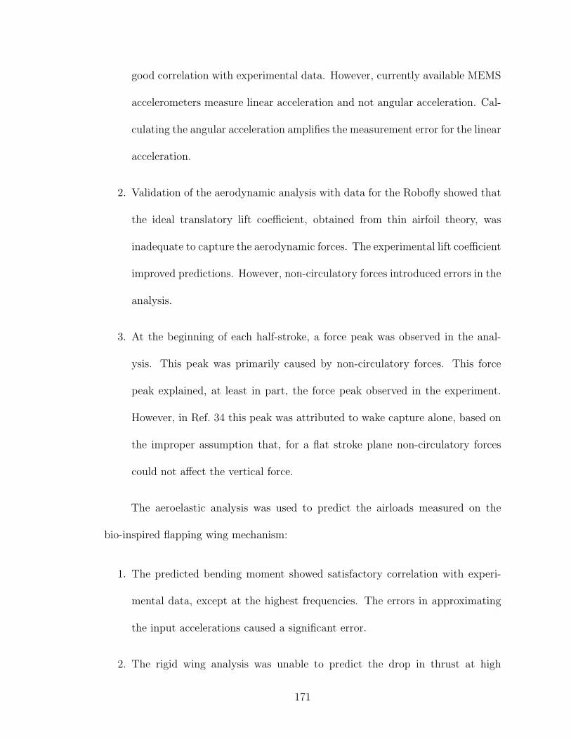
good correlation with experimental data. However, currently available MEMS

accelerometers measure linear acceleration and not angular acceleration. Cal-

culating the angular acceleration amplifies the measurement error for the linear

acceleration.

2. Validation of the aerodynamic analysis with data for the Robofly showed that

the ideal translatory lift coefficient, obtained from thin airfoil theory, was

inadequate to capture the aerodynamic forces. The experimental lift coefficient

improved predictions. However, non-circulatory forces introduced errors in the

analysis.

3. At the beginning of each half-stroke, a force peak was observed in the anal-

ysis. This peak was primarily caused by non-circulatory forces. This force

peak explained, at least in part, the force peak observed in the experiment.

However, in Ref. 34 this peak was attributed to wake capture alone, based on

the improper assumption that, for a flat stroke plane non-circulatory forces

could not affect the vertical force.

The aeroelastic analysis was used to predict the airloads measured on the

bio-inspired flapping wing mechanism:

1. The predicted bending moment showed satisfactory correlation with experi-

mental data, except at the highest frequencies. The errors in approximating

the input accelerations caused a significant error.

2. The rigid wing analysis was unable to predict the drop in thrust at high

171

frequency. However, the elastic analysis predicted this drop.

3. Wing elasticity led to a significant increase in the circulatory thrust because

of the higher effective wing velocity. However, this increase was offset by

a reduction in the thrust produced by non-circulatory forces. In fact, it is

this reduction that caused the drop in thrust at high frequency. As the non-

circulatory thrust dropped, the overall thrust and hence the inflow velocity,

reduced. This brought the shed wake close to the wing, leading to large oscil-

lations in the thrust and no convergence.

4. The bending moment error at a high frequency was found to be caused by the

duration of wing acceleration in a flapping cycle. With an improvement in

bending moment prediction, the thrust prediction was also improved.

5. A coupled analysis did not have significant effect on the average thrust. While

the overall variation of the bending moment was adequately captured by the

uncoupled analysis, the aerodynamic coupling introduced significant changes.

This shows that the aerodynamic loads cannot be neglected to obtain the wing

response accurately.

7.2 Important Contributions

The following are the major contributions of this research work:

1. Prior to this study there was no experimental data available for hover capable

flapping wings at the Reynolds numbers and flapping frequencies relevant to

172

MAV development. This gap has been addressed to some extent by the present

work.

2. The experimental challenges involved, such as, measurement of the small aero-

dynamic forces in the presence of large inertial loads, were addressed. Custom

built force and motion transducers were used because of the need for small,

sensitive and light-weight sensors.

3. Aeroelastic studies on wings undergoing large amplitude flapping and pitching

motions, in the hover mode, were non-existent in literature. The development

and validation of the aeroelastic analysis addressed this issue.

4. Wing aeroelasticity was found to be a major barrier in achieving high thrust

from bio-inspired flapping. This underscores the importance of systematic

structural and aeroelastic design of the wings.

5. A novel mechanism based on passive pitching of the wing, caused by aeroelastic

forces, was also investigated. This type of flapping shows some promise for

MAV development because of its mechanical simplicity and high thrust.

7.3 Recommendations for Future Work

This dissertation describes a small step in the development of flapping wing

MAVs which are still in their infancy. A considerable amount of work remains to be

done before such MAVs are practically realized. The following are some directions

along which further research can be carried out:

173

1. The aerodynamic model may be improved using an unsteady vortex lattice

method. When coupled with the structural model, this analysis can be used

to optimize the structural and aerodynamic design of the wing.

2. The structural model can be coupled with a CFD analysis to obtain greater

accuracy in aerodynamic computations. The ultimate goal being a fluid struc-

ture interaction model with a non-linear, multi-body structural analysis and

a CFD based aerodynamic analysis.

3. From an implementation standpoint, the design of the mechanism is the key

issue. In order to achieve tethered flight a passive pitch mechanism might

be the simplest mechanism. The stiffness of the torsion spring and the mass

distribution of the wing may be optimized in order to obtain a wing motion

that is as close to bio-inspired flapping as possible.

4. On the experimental side, the flapping wing mechanism can be used to study

wings in forward flight and also under gusts. This will help in validating the

above analyses under different flight conditions.

5. Ultimately, using the dragonfly as a model, wing-wing interactions may be

studied using the analytical tools developed in order to see whether these

interactions can be beneficial to the design of an MAV.

174

Appendix A

Finite Element Matrices

A.1 Shape function matrices

Bi-linear shape functions for in-plane deformations,

n1 =1

4(1− ξ)(1− η) (A.1)

n2 =1

4(1 + ξ)(1− η) (A.2)

n3 =1

4(1 + ξ)(1 + η) (A.3)

n4 =1

4(1− ξ)(1 + η) (A.4)

{N1} = [n1 n2 n3 n4 {0}1×20] (A.5)

{N1} = [{0}1×4 n1 n2 n3 n4 {0}1×16] (A.6)

where, ξ = xa

and η = yb.

175

{N3} =1

16a3b3

{0}8×1

(y + 2 b) (−b+ y)2 (2 a+ x) (a− x)2

(y + 2 b) (−b+ y)2 (a+ x) (a− x)2 a

(y + b) (−b+ y)2 (2 a+ x) (a− x)2 b

(y + b) (−b+ y)2 (a+ x) (a− x)2 ab

(y + 2 b) (−b+ y)2 (2 a− x) (a+ x)2

− (y + 2 b) (−b+ y)2 (a− x) (a+ x)2 a

(y + b) (−b+ y)2 (2 a− x) (a+ x)2 b

− (y + b) (−b+ y)2 (a− x) (a+ x)2 ab

− (−2 b+ y) (y + b)2 (2 a− x) (a+ x)2

(−2 b+ y) (y + b)2 (a− x) (a+ x)2 a

(−b+ y) (y + b)2 (2 a− x) (a+ x)2 b

− (−b+ y) (y + b)2 (a− x) (a+ x)2 ab

− (−2 b+ y) (y + b)2 (2 a+ x) (a− x)2

− (−2 b+ y) (y + b)2 (a+ x) (a− x)2 a

(−b+ y) (y + b)2 (2 a+ x) (a− x)2 b

(−b+ y) (y + b)2 (a+ x) (a− x)2 ab

T

(A.7)

176

A.2 Dynamic stiffening matrices

∫ x

−a[N3,x]

T [N3,x]dx =1

3840a6b6

[9C12C3

4C6 −32aC1

2C34C7 9 bC1 C3

4C4 C6 −32abC1 C3

4C4 C7

−9C12C3

4C632aC1

2C34C9 −9 bC1 C3

4C4 C632abC1 C3

4C4 C9

9C32C4

2C6 C5 −32aC3

2C42C9 C5 −9 bC1 C3

3C42C6

32abC1 C3

3C42C9

−9C32C4

2C6 C532aC3

2C42C7 C5 9 bC1 C3

3C42C6 −3

2abC1 C3

3C42C7 ]

[−32aC1

2C34C7 a2C1

2C34C8 −3

2abC1 C3

4C4 C7 a2bC1 C34C4 C8

32aC1

2C34C7 −a2C1

2C34C10

32abC1 C3

4C4 C7 −a2bC1 C34C4 C10

−32aC3

2C42C7 C5 a2C3

2C42C10 C5

32abC1 C3

3C42C7 −a2bC1 C3

3C42C10

32aC3

2C42C7 C5 −a2C3

2C42C8 C5 −3

2abC1 C3

3C42C7 a2bC1 C3

3C42C8 ]

[9 bC1 C34C4 C6 −3

2abC1 C3

4C4 C7 9 b2C42C3

4C6 −32ab2C4

2C34C7

−9 bC1 C34C4 C6

32abC1 C3

4C4 C9 −9 b2C42C3

4C632ab2C4

2C34C9

9 bC43C3

2C2 C6 −32abC4

3C32C2 C9 −9 b2C4

3C33C6

32ab2C4

3C33C9

−9 bC43C3

2C2 C632abC4

3C32C2 C7 9 b2C4

3C33C6 −3

2ab2C4

3C33C7 ]

[−32abC1 C3

4C4 C7 a2bC1 C34C4 C8 −3

2ab2C4

2C34C7 a2b2C4

2C34C8

32abC1 C3

4C4 C7 −a2bC1 C34C4 C10

32ab2C4

2C34C7 −a2b2C4

2C34C10

−32abC4

3C32C2 C7 a2bC4

3C32C2 C10

32ab2C4

3C33C7 −a2b2C4

3C33C10

32abC4

3C32C2 C7 −a2bC4

3C32C2 C8 −3

2ab2C4

3C33C7 a2b2C4

3C33C8 ]

177

[−9C12C3

4C632aC1

2C34C7 −9 bC1 C3

4C4 C632abC1 C3

4C4 C7

9C12C3

4C6 −32aC1

2C34C9 9 bC1 C3

4C4 C6 −32abC1 C3

4C4 C9

−9C32C4

2C6 C532aC3

2C42C9 C5 9 bC1 C3

3C42C6 −3

2abC1 C3

3C42C9

9C32C4

2C6 C5 −32aC3

2C42C7 C5 −9 bC1 C3

3C42C6

32abC1 C3

3C42C7 ]

[32aC1

2C34C9 −a2C1

2C34C10

32abC1 C3

4C4 C9 −a2bC1 C34C4 C10

−32aC1

2C34C9 a2C1

2C34C11 −3

2abC1 C3

4C4 C9 a2bC1 C34C4 C11

32aC3

2C42C9 C5 −a2C3

2C42C11 C5 −3

2abC1 C3

3C42C9 a2bC1 C3

3C42C11

−32aC3

2C42C9 C5 a2C3

2C42C10 C5

32abC1 C3

3C42C9 −a2bC1 C3

3C42C10 ]

[−9 bC1 C34C4 C6

32abC1 C3

4C4 C7 −9 b2C42C3

4C632ab2C4

2C34C7

9 bC1 C34C4 C6 −3

2abC1 C3

4C4 C9 9 b2C42C3

4C6 −32ab2C4

2C34C9

−9 bC43C3

2C2 C632abC4

3C32C2 C9 9 b2C4

3C33C6 −3

2ab2C4

3C33C9

9 bC43C3

2C2 C6 −32abC4

3C32C2 C7 −9 b2C4

3C33C6

32ab2C4

3C33C7 ]

[32abC1 C3

4C4 C9 −a2bC1 C34C4 C10

32ab2C4

2C34C9 −a2b2C4

2C34C10

−32abC1 C3

4C4 C9 a2bC1 C34C4 C11 −3

2ab2C4

2C34C9 a2b2C4

2C34C11

32abC4

3C32C2 C9 −a2bC4

3C32C2 C11 −3

2ab2C4

3C33C9 a2b2C4

3C33C11

−32abC4

3C32C2 C9 a2bC4

3C32C2 C10

32ab2C4

3C33C9 −a2b2C4

3C33C10 ]

[9C32C4

2C6 C5 −32aC3

2C42C7 C5 9 bC4

3C32C2 C6 −3

2abC4

3C32C2 C7

−9C32C4

2C6 C532aC3

2C42C9 C5 −9 bC4

3C32C2 C6

32abC4

3C32C2 C9

9C22C4

4C6 −32aC2

2C44C9 −9 bC3 C4

4C2 C632abC2 C4

4C3 C9

−9C22C4

4C632aC2

2C44C7 9 bC3 C4

4C2 C6 −32abC3 C4

4C2 C7 ]

178

[−32aC3

2C42C9 C5 a2C3

2C42C10 C5 −3

2abC4

3C32C2 C9 a2bC4

3C32C2 C10

32aC3

2C42C9 C5 −a2C3

2C42C11 C5

32abC4

3C32C2 C9 −a2bC4

3C32C2 C11

−32aC2

2C44C9 a2C2

2C44C11

32abC2 C4

4C3 C9 −a2bC2 C44C3 C11

32aC2

2C44C9 −a2C2

2C44C10 −3

2abC2 C4

4C3 C9 a2bC3 C44C2 C10 ]

[−9 bC1 C33C4

2C632abC1 C3

3C42C7 −9 b2C4

3C33C6

32ab2C4

3C33C7

9 bC1 C33C4

2C6 −32abC1 C3

3C42C9 9 b2C4

3C33C6 −3

2ab2C4

3C33C9

−9 bC3 C44C2 C6

32abC2 C4

4C3 C9 9 b2C32C4

4C6 −32ab2C3

2C44C9

9 bC3 C44C2 C6 −3

2abC3 C4

4C2 C7 −9 b2C32C4

4C632ab2C3

2C44C7 ]

[32abC1 C3

3C42C9 −a2bC1 C3

3C42C10

32ab2C4

3C33C9 −a2b2C4

3C33C10

−32abC1 C3

3C42C9 a2bC1 C3

3C42C11 −3

2ab2C4

3C33C9 a2b2C4

3C33C11

32abC2 C4

4C3 C9 −a2bC2 C44C3 C11 −3

2ab2C3

2C44C9 a2b2C3

2C44C11

−32abC2 C4

4C3 C9 a2bC3 C44C2 C10

32ab2C3

2C44C9 −a2b2C3

2C44C10 ]

[−9C32C4

2C6 C532aC3

2C42C7 C5 −9 bC4

3C32C2 C6

32abC4

3C32C2 C7

9C32C4

2C6 C5 −32aC3

2C42C9 C5 9 bC4

3C32C2 C6 −3

2abC4

3C32C2 C9

−9C22C4

4C632aC2

2C44C9 9 bC3 C4

4C2 C6 −32abC2 C4

4C3 C9

9C22C4

4C6 −32aC2

2C44C7 −9 bC3 C4

4C2 C632abC3 C4

4C2 C7 ]

[32aC3

2C42C7 C5 −a2C3

2C42C8 C5

32abC4

3C32C2 C7 −a2bC4

3C32C2 C8

−32aC3

2C42C7 C5 a2C3

2C42C10 C5 −3

2abC4

3C32C2 C7 a2bC4

3C32C2 C10

32aC2

2C44C7 −a2C2

2C44C10 −3

2abC3 C4

4C2 C7 a2bC3 C44C2 C10

−32aC2

2C44C7 a2C2

2C44C8

32abC3 C4

4C2 C7 −a2bC2 C44C3 C8 ]

179

[9 bC1 C33C4

2C6 −32abC1 C3

3C42C7 9 b2C4

3C33C6 −3

2ab2C4

3C33C7

−9 bC1 C33C4

2C632abC1 C3

3C42C9 −9 b2C4

3C33C6

32ab2C4

3C33C9

9 bC3 C44C2 C6 −3

2abC2 C4

4C3 C9 −9 b2C32C4

4C632ab2C3

2C44C9

−9 bC3 C44C2 C6

32abC3 C4

4C2 C7 9 b2C32C4

4C6 −32ab2C3

2C44C7 ]

[−32abC1 C3

3C42C7 a2bC1 C3

3C42C8 −3

2ab2C4

3C33C7 a2b2C4

3C33C8

32abC1 C3

3C42C7 −a2bC1 C3

3C42C10

32ab2C4

3C33C7 −a2b2C4

3C33C10

−32abC3 C4

4C2 C7 a2bC3 C44C2 C10

32ab2C3

2C44C7 −a2b2C3

2C44C10

32abC3 C4

4C2 C7 −a2bC2 C44C3 C8 −3

2ab2C3

2C44C7 a2b2C3

2C44C8 ]

(A.8)

where,

C1 = y + 2 b (A.9)

C2 = −2 b+ y (A.10)

C3 = −b+ y (A.11)

C4 = y + b (A.12)

C5 = y2 − 4 b2 (A.13)

C6 = 3 x 5 + 8 a5 − 10 a2x 3 + 15 a4x (A.14)

C7 = −18 x 5 + 7 a5 + 15 ax 4 + 40 a2x 3 − 30 a3x 2 − 30 a4x (A.15)

C8 = 27 x 5 + 47 a5 − 45 ax 4 − 10 a2x 3 + 30 a3x 2 + 15 a4x (A.16)

C9 = 18 x 5 + 23 a5 + 15 ax 4 − 40 a2x 3 − 30 a3x 2 + 30 a4x (A.17)

180

C10 = −27 x 5 + 8 a5 + 50 a2x 3 − 15 a4x (A.18)

C11 = 27 x 5 + 17 a5 + 45 ax 4 − 10 a2x 3 − 30 a3x 2 + 15 a4x ] (A.19)

∫ y

−b[N3,y]

T [N3,y]dy =1

3840a6b6

[9D12D4

4D7 9 aD5 D44D1 D7 −3

2bD1

2D44D8 −3

2abD5 D4

4D1 D8

9D42D5

2D7 D6 −9 aD43D5

2D1 D7 −32bD4

2D52D8 D6

32abD4

3D52D1 D8

−9D42D5

2D7 D6 9 aD43D5

2D1 D732bD4

2D52D9 D6 −3

2abD4

3D52D1 D9

−9D12D4

4D7 −9 aD5 D44D1 D7

32bD1

2D44D9

32abD5 D4

4D1 D9 ]

[9 aD5 D44D1 D7 9 a2D5

2D44D7 −3

2abD5 D4

4D1 D8 −32a2bD5

2D44D8

9 aD3 D53D4

2D7 −9 a2D43D5

3D7 −32abD3 D5

3D42D8

32a2bD4

3D53D8

−9 aD3 D53D4

2D7 9 a2D43D5

3D732abD3 D5

3D42D9 −3

2a2bD4

3D53D9

−9 aD5 D44D1 D7 −9 a2D5

2D44D7

32abD5 D4

4D1 D932a2bD5

2D44D9 ]

[−32bD1

2D44D8 −3

2abD5 D4

4D1 D8 b2D12D4

4D12 ab2D5 D44D1 D12

−32bD4

2D52D8 D6

32abD4

3D52D1 D8 b2D4

2D52D12 D6 −ab2D4

3D52D1 D12

32bD4

2D52D8 D6 −3

2abD4

3D52D1 D8 −b2D4

2D52D11 D6 ab2D4

3D52D1 D11

32bD1

2D44D8

32abD5 D4

4D1 D8 −b2D12D4

4D11 −ab2D5 D44D1 D11 ]

[−32abD5 D4

4D1 D8 −32a2bD5

2D44D8 ab2D5 D4

4D1 D12 a2b2D52D4

4D12

−32abD3 D5

3D42D8

32a2bD4

3D53D8 ab2D5

3D42D3 D12 −a2b2D4

3D53D12

32abD3 D5

3D42D8 −3

2a2bD4

3D53D8 −ab2D5

3D42D3 D11 a2b2D4

3D53D11

32abD5 D4

4D1 D832a2bD5

2D44D8 −ab2D5 D4

4D1 D11 −a2b2D52D4

4D11 ]

181

[9D42D5

2D7 D6 9 aD3 D53D4

2D7 −32bD4

2D52D8 D6 −3

2abD3 D5

3D42D8

9D32D5

4D7 −9 aD4 D54D3 D7 −3

2bD3

2D54D8

32abD4 D5

4D3 D8

−9D32D5

4D7 9 aD4 D54D3 D7

32bD3

2D54D9 −3

2abD4 D5

4D3 D9

−9D42D5

2D7 D6 −9 aD3 D53D4

2D732bD4

2D52D9 D6

32abD3 D5

3D42D9 ]

[−9 aD43D5

2D1 D7 −9 a2D43D5

3D732abD4

3D52D1 D8

32a2bD4

3D53D8

−9 aD4 D54D3 D7 9 a2D4

2D54D7

32abD4 D5

4D3 D8 −32a2bD4

2D54D8

9 aD4 D54D3 D7 −9 a2D4

2D54D7 −3

2abD4 D5

4D3 D932a2bD4

2D54D9

9 aD43D5

2D1 D7 9 a2D43D5

3D7 −32abD4

3D52D1 D9 −3

2a2bD4

3D53D9 ]

[−32bD4

2D52D8 D6 −3

2abD3 D5

3D42D8 b2D4

2D52D12 D6 ab2D5

3D42D3 D12

−32bD3

2D54D8

32abD4 D5

4D3 D8 b2D32D5

4D12 −ab2D4 D54D3 D12

32bD3

2D54D8 −3

2abD4 D5

4D3 D8 −b2D32D5

4D11 ab2D4 D54D3 D11

32bD4

2D52D8 D6

32abD3 D5

3D42D8 −b2D4

2D52D11 D6 −ab2D5

3D42D3 D11 ]

[32abD4

3D52D1 D8

32a2bD4

3D53D8 −ab2D4

3D52D1 D12 −a2b2D4

3D53D12

32abD4 D5

4D3 D8 −32a2bD4

2D54D8 −ab2D4 D5

4D3 D12 a2b2D42D5

4D12

−32abD4 D5

4D3 D832a2bD4

2D54D8 ab2D4 D5

4D3 D11 −a2b2D42D5

4D11

−32abD4

3D52D1 D8 −3

2a2bD4

3D53D8 ab2D4

3D52D1 D11 a2b2D4

3D53D11 ]

[−9D42D5

2D7 D6 −9 aD3 D53D4

2D732bD4

2D52D8 D6

32abD3 D5

3D42D8

−9D32D5

4D7 9 aD4 D54D3 D7

32bD3

2D54D8 −3

2abD4 D5

4D3 D8

9D32D5

4D7 −9 aD4 D54D3 D7 −3

2bD3

2D54D9

32abD4 D5

4D3 D9

9D42D5

2D7 D6 9 aD3 D53D4

2D7 −32bD4

2D52D9 D6 −3

2abD3 D5

3D42D9 ]

182

[9 aD43D5

2D1 D7 9 a2D43D5

3D7 −32abD4

3D52D1 D8 −3

2a2bD4

3D53D8

9 aD4 D54D3 D7 −9 a2D4

2D54D7 −3

2abD4 D5

4D3 D832a2bD4

2D54D8

−9 aD4 D54D3 D7 9 a2D4

2D54D7

32abD4 D5

4D3 D9 −32a2bD4

2D54D9

−9 aD43D5

2D1 D7 −9 a2D43D5

3D732abD4

3D52D1 D9

32a2bD4

3D53D9 ]

[32bD4

2D52D9 D6

32abD3 D5

3D42D9 −b2D4

2D52D11 D6 −ab2D5

3D42D3 D11

32bD3

2D54D9 −3

2abD4 D5

4D3 D9 −b2D32D5

4D11 ab2D4 D54D3 D11

−32bD3

2D54D9

32abD4 D5

4D3 D9 b2D32D5

4D10 −ab2D4 D54D3 D10

−32bD4

2D52D9 D6 −3

2abD3 D5

3D42D9 b2D4

2D52D10 D6 ab2D5

3D42D3 D10 ]

[−32abD4

3D52D1 D9 −3

2a2bD4

3D53D9 ab2D4

3D52D1 D11 a2b2D4

3D53D11

−32abD4 D5

4D3 D932a2bD4

2D54D9 ab2D4 D5

4D3 D11 −a2b2D42D5

4D11

32abD4 D5

4D3 D9 −32a2bD4

2D54D9 −ab2D4 D5

4D3 D10 a2b2D42D5

4D10

32abD4

3D52D1 D9

32a2bD4

3D53D9 −ab2D4

3D52D1 D10 −a2b2D4

3D53D10 ]

[−9D12D4

4D7 −9 aD5 D44D1 D7

32bD1

2D44D8

32abD5 D4

4D1 D8

−9D42D5

2D7 D6 9 aD43D5

2D1 D732bD4

2D52D8 D6 −3

2abD4

3D52D1 D8

9D42D5

2D7 D6 −9 aD43D5

2D1 D7 −32bD4

2D52D9 D6

32abD4

3D52D1 D9

9D12D4

4D7 9 aD5 D44D1 D7 −3

2bD1

2D44D9 −3

2abD5 D4

4D1 D9 ]

[−9 aD5 D44D1 D7 −9 a2D5

2D44D7

32abD5 D4

4D1 D832a2bD5

2D44D8

−9 aD3 D53D4

2D7 9 a2D43D5

3D732abD3 D5

3D42D8 −3

2a2bD4

3D53D8

9 aD3 D53D4

2D7 −9 a2D43D5

3D7 −32abD3 D5

3D42D9

32a2bD4

3D53D9

9 aD5 D44D1 D7 9 a2D5

2D44D7 −3

2abD5 D4

4D1 D9 −32a2bD5

2D44D9 ]

183

[32bD1

2D44D9

32abD5 D4

4D1 D9 −b2D12D4

4D11 −ab2D5 D44D1 D11

32bD4

2D52D9 D6 −3

2abD4

3D52D1 D9 −b2D4

2D52D11 D6 ab2D4

3D52D1 D11

−32bD4

2D52D9 D6

32abD4

3D52D1 D9 b2D4

2D52D10 D6 −ab2D4

3D52D1 D10

−32bD1

2D44D9 −3

2abD5 D4

4D1 D9 b2D12D4

4D10 ab2D5 D44D1 D10 ]

[32abD5 D4

4D1 D932a2bD5

2D44D9 −ab2D5 D4

4D1 D11 −a2b2D52D4

4D11

32abD3 D5

3D42D9 −3

2a2bD4

3D53D9 −ab2D5

3D42D3 D11 a2b2D4

3D53D11

−32abD3 D5

3D42D9

32a2bD4

3D53D9 ab2D5

3D42D3 D10 −a2b2D4

3D53D10

−32abD5 D4

4D1 D9 −32a2bD5

2D44D9 ab2D5 D4

4D1 D10 a2b2D52D4

4D10 ]

(A.20)

where,

D1 = 2 a+ x (A.21)

D2 = x− 2 a (A.22)

D3 = 2 a− x (A.23)

D4 = a− x (A.24)

D5 = a+ x (A.25)

D6 = 4 a2 − x2 (A.26)

D7 = 3 y5 + 8 b5 − 10 b2y3 + 15 b4y (A.27)

D8 = −18 y5 + 7 b5 + 15 by4 + 40 b2y3 − 30 b3y2 − 30 b4y (A.28)

D9 = 18 y5 + 23 b5 + 15 by4 − 40 b2y3 − 30 b3y2 + 30 b4y (A.29)

184

D10 = 27 y5 + 17 b5 + 45 by4 − 10 b2y3 − 30 b3y2 + 15 b4y (A.30)

D11 = −27 y5 + 8 b5 + 50 b2y3 − 15 b4y (A.31)

D12 = 27 y5 + 47 b5 − 45 by4 − 10 b2y3 + 30 b3y2 + 15 b4y ] (A.32)

185

Appendix B

Aerodynamic Expressions

B.1 Non-circulatory force

The rigid part of the non-circulatory force is given by,

F rigidnc =

1

4ρ c2π

(− 3 Vh sin θ − 3Vh cos θ

dθ

dt− 3 Vv cos θ

+3Vv sin θdθ

dt− 2 c

d2θ

dt2+ 3 ac

d2θ

dt2

)(B.1)

The elastic part of the non-circulatory force is given by,

F elasticnc =

1

4ρ c2

Nm∑p=1

(− 3B

′p0 qpVh cos θ − 3Bp

0 qp

−3B′p0 qp cos θVh + 3B

′p0 qpVh sin θθ + 3B

′p0 qpVv sin θ

+3B′p0 qpVv cos θθ + 3B

′p0 qpVv sin θ + 2Bp

1 qp

+2B′p1 qp cos θVh − 2B

′p1 qpVh sin θθ − 2B

′p1 qpVv sin θ

−2B′p1 qpVv cos θθ + 2B

′p1 qpVh cos θ − 2B

′p1 qpVv sin θ

+Bp2 qp + B

′p2 qp cos θVh − B

′p2 qpVh sin θθ − B

′p2 qpVv sin θ

186

−B′p2 qpVv cos θθ + B

′p2 qpVh cos θ − B

′p2 qpVv sin θ

)(B.2)

B.2 Circulation

(dΓ

dt

)rigid

= −1

4, π c

(− 4 Vh sin θ − 4Vh cos θ θ − 4 Vv cos θ

+4Vv sin θ θ − 3 cθ + 4 cθ a)

(B.3)

(dΓ

dt

)elastic

= cNm∑p=1

(−Bp

0 qp −B′p0 qp Vh cos θ −B

′p0 qpVh cos θ

+B′p0 qpVh sin θ θ +B

′p0 qpp Vv sin θ +B

′p0 qpVv sin θ

+B′p0 qpVv (t) cos θ θ +Bp

1 qp +B′p1 qp Vh cos θ

+B′p1 qpVh cos θ −B

′p1 qpVh sin θ θ −B

′p1 qp Vv sin θ

−B′p1 qpVv sin θ −B

′p1 qpVv cos θ θ

)(B.4)

187

BIBLIOGRAPHY

[1] McMichael, J. M. and Francis, M. S., Micro Air Vehicles - Toward a NewDimension in Flight , Defence Advanced Research Projects Agency TTO Doc-ument, 1996.

[2] Barret, C., “Aerobots and Hydrobots for Planetary Exploration,” 38th AIAAAerospace Sciences Meeting and Exhibit , Reno, Nevada, January 10-13 2000.

[3] Tarascio, M. J. and Chopra, I., “Design and Development of a Thrust Aug-mented Entomopter : An Advanced Flapping Wing Micro Hovering Air Ve-hicle,” Proceedings of the 59th Annual Forum of the American Helicopter So-ciety , Phoenix, AZ, May 2003.

[4] Grasmeyer, J. M. and Keennon, M. T., “Development of the Black WidowMicro Air Vehicle,” 39th AIAA Aerospace Sciences Meeting and Exhibit , Reno,Nevada, January 8-11 2001.

[5] Keennon, M. T. and Grasmeyer, J. M., “Development of the Black Widowand Microbat MAVs and a Vision of the Future of MAV Design,” AIAA/ICASInternational Air and Space Symposium and Exposition: The Next 100 Years ,Dayton, Ohio, July 14-17 2003.

[6] Gyllhem, D., Mohseni, K., Lawrence, D., and Geuzaine, P., “Numerical Sim-ulation of Flow Around the Colorado Micro Aerial Vehicle,” 35th AIAA FluidDynamics Conference and Exhibit , Toronto, Ontario, Canada, June 6-9 2005.

[7] Ifju, P. G., Jenkins, D. A., Ettinger, S., Lian, Y., Shyy, W., and Waszak,M. R., “Flexible-Wing-Based Micro Air Vehicles,” 40th AIAA Aerospace Sci-ences Meeting and Exhibit , Reno, Nevada, January 14-17 2002.

[8] Petersen, B., Erath, B., Henry, K., Lyon, M., Walker, B., Powell, N., Fowkes,K., and Bowman, W. J., “Development of a Micro Air Vehicle for MaximumEndurance and Minimum Size,” 41st AIAA Aerospace Sciences Meeting andExhibit , Reno, Nevada, January 6-9 2003.

[9] Brion, V., Aki, M., and Shkarayev, S., “Numerical Simulations of LowReynolds Number Flows Around Micro Air Vehicles and Comparison againstWind Tunnel Data,” 24th AIAA Applied Aerodynamics Conference, San Fran-cisco, California, June 5-8 2006.

[10] Lian, Y. and Shyy, W., “Numerical Simulations of Membrane Wing Aero-dynamics for Micro Air Vehicle Applications,” Journal of Aircraft , Vol. 42,No. 4, July-August 2005, pp. 865–873.

[11] Stanford, B., Viieru, D., Albertani, R., Shyy, W., and Ifju, P., “A Numericaland Experimental Investigation of Flexible Micro Air Vehicle Wing Defor-mation,” 44th AIAA Aerospace Sciences Meeting and Exhibit , Reno, Nevada,January 9-12 2006.

188

[12] Viieru, D., Albertani, R., Shyy, W., and Ifju, P. G., “Effect of Tip Vortexon Wing Aerodynamics of Micro Air Vehicles,” Journal of Aircraft , Vol. 42,No. 6, November-December 2005, pp. 1530–1536.

[13] Abdulrahim, M., Garcia, H., and Lind, R., “Analysis and estimation of the liftcomponents of hovering insects,” Journal of Aircraft , Vol. 42, No. 1, January-February 2005, pp. 131–137.

[14] Abdulrahim, M., Garcia, H., Ivey, G. F., and Lind, R., “Flight TestingA Micro Air Vehicle Using Morphing For Aeroservoelastic Control,” 45th

AIAA/ASME/ASCE/AHS/ASC SDM conference, Palm Springs, California,April 19-22 2004.

[15] DeLuca, A. M., Reeder, M. F., OL, M. V., Freeman, J., Bautista, I., andSimonich, M., “Experimental Investigation into the Aerodynamic Propertiesof a Flexible and Rigid Wing Micro Air Vehicle,” 24th AIAA AerodynamicMeasurement Technology and Ground Testing Conference, Portland, Oregon,June 28 - July 1 2004.

[16] DeLuca, A. M., Reeder, M. F., Freeman, J., and OL, M. V., “Flexible andRigid-Wing Micro Air Vehicle: Lift and Drag Comparison,” Journal of Air-craft , Vol. 43, No. 2, March-April 2006, pp. 572–575.

[17] Garcia, H. M., Abdulrahim, M., and Lind, R., “Roll Control for a MicroAir Vehicle Using Active Wing Morphing,” AIAA Guidance, Navigation andControl Conference and Exhibit , Austin, Texas, August 11-14 2003.

[18] Bohorquez, F. and Pines, D., “Hover Performance of Rotor Blades at LowReynolds Numbers for Rotary Wing Micro Air Vehicles,” 2nd AIAA ”Un-manned Unlimited” Systems, Technologies and Operations Conference andWorkshop, San Diego, California, September 15-18 2003.

[19] Bohorquez, F., Rankins, F., Baeder, J. D., and Pines, D., “Hover Perfor-mance of Rotor Blades at Low Reynolds Numbers for Rotary Wing MicroAir Vehicles. An Experimental and CFD Study,” 21st Applied AerodynamicsConference, Orlando, Florida, June 23-26 2003.

[20] Ramasamy, M., Leishman, J. G., and Lee, T. E., “Flow Field of a Rotating-Wing Micro Air Vehicle,” 62nd Annual Forum of the American HelicopterSociety , Phoenix, AZ, May 9-11 2006.

[21] Lakshminarayan, V. K., Bush, B. L., Duraisamy, K., and Baeder, J. D., “Com-putational Investigation of Micro Hovering Rotor Aerodynamics,” 24th AIAAApplied Aerodynamics Conference, San Francisco, California, June 5-8 2006.

[22] Conroy, J. K., Samuel, P. D., and Pines, D. J., “Development of an MAVControl and Navigation System,” Infotech@Aerospace, Arlington, Virginia,September 26-29 2005.

189

[23] Pines, D. J. and Bohorquez, F., “Challenges Facing Future Micro-Air-VehicleDevelopment,” Journal of Aircraft , Vol. 43, No. 2, March-April 2006, pp. 290–305.

[24] Akle, B. J. and Leo, D. J., “Consideration of Ionic PolymerMaterials as Flapping Mechanisms for Micro-Air Vehicles,” 44th

AIAA/ASME/ASCE/AHS/ASC SDM conference, Norfolk, Virginia, April7-10 2003.

[25] Shyy, W., Berg, M., and Ljungqvist, D., “Flapping and Flexible Wings forBiological and Micro Air Vehicles,” Progress in Aerospace Sciences , Vol. 35,No. 5, July 1999, pp. 455–505.

[26] Weis-fogh, T., “Quick Estimates of Flight Fitness in Hovering Animals, Includ-ing Novel Mechanisms for Lift Production,” Journal of Experimental Biology ,Vol. 59, No. 1, 1973, pp. 169–230.

[27] Ellington, C. P., “The Aerodynamics of Hovering Insect Flight,” PhilosophicalTransactions of the Royal Society of London Series B , Vol. 305, No. 1122,February 1984, pp. 1–181.

[28] Willmott, A. P. and Ellington, C. P., “The Mechanics of Flight in the Hawk-moth Manduca Sexta I. Kinematics of Hovering and Forward Flight,” Journalof Experimental Biology , Vol. 200, 1997, pp. 2705–2722.

[29] Altshuler, D. L. and Dudley, R., “Kinematics of Hovering Hummingbird FlightAlong Simulated and Natural Elevational Gradients,” Journal of ExperimentalBiology , Vol. 206, 2003, pp. 3139–3147.

[30] Wang, H., Zeng, L., Liu, H., and Yin, C., “Measuring Wing Kinematics, FlightTrajectory and Body Attitude During Forward Flight and Turning Maneuversin Dragonflies,” Journal of Experimental Biology , Vol. 206, 2003, pp. 745–757.

[31] Dickinson, M. H. and Gotz, K. G., “Unsteady Aerodynamic Performance ofModel Wings at Low Reynolds Numbers,” Journal of Experimental Biology ,Vol. 174, 1993, pp. 45–64.

[32] van den Berg, C. and Ellington, C. P., “The Vortex Wake of a ”Hovering”Model Hawkmoth,” Philosophical Transactions: Biological Sciences , Vol. 352,No. 1351, March 1997, pp. 317–328.

[33] van den Berg, C. and Ellington, C. P., “The Three-Dimensional Leading-Edge Vortex of a ”Hovering” Model Hawkmoth,” Philosophical Transactions:Biological Sciences , Vol. 352, No. 1351, March 1997, pp. 329–340.

[34] Dickinson, M. H., Lehmann, F., and Sane, S. P., “Wing Rotation and theAerodynamic Basis of Insect Flight,” Science, Vol. 284, June 1999, pp. 1954–1960.

190

[35] Willmott, A. P. and Ellington, C. P., “The Mechanics of Flight in theHawkmoth Manduca Sexta II. Aerodynamic Consequences of Kinematic andMorphological Variation,” Journal of Experimental Biology , Vol. 200, 1997,pp. 2723–2745.

[36] Liu, T., “Comparative Scaling of Flapping- and Fixed-Wing Flyers,” AIAAJournal , Vol. 44, No. 1, January 2006, pp. 24–33.

[37] Spedding, G. R., Rosen, M., and Hedenstrom, A., “A family of vortex wakesgenerated by a thrush nightingale in free flight in a wind tunnel over its entirenatural range of flight speeds,” Journal of Experimental Biology , Vol. 206,2003, pp. 2313–2344.

[38] Usherwood, J. R., Hedrick, T. L., and Biewener, A. A., “The aerodynamicsof avian take-off from direct pressure measurements in Canada geese (Brantacanadensis),” Journal of Experimental Biology , Vol. 206, 2003, pp. 4051–4056.

[39] Hedrick, T. L., Usherwood, J. R., and Biewener, A. A., “Wing inertia andwhole-body acceleration: an analysis of instantaneous aerodynamic force pro-duction in cockatiels (Nymphicus hollandicus) flying across a range of speeds,”Journal of Experimental Biology , Vol. 207, 2004, pp. 1689–1702.

[40] Usherwood, J. R., Hedrick, T. L., McGowan, C. P., and Biewener, A. A.,“Dynamic pressure maps for wings and tails of pigeons in slow, flapping flight,and their energetic implications,” Journal of Experimental Biology , Vol. 208,2005, pp. 355–369.

[41] Srygley, R. B. and Thomas, A. L. R., “Unconventional Lift Generating Mech-anisms in Free-Flying Butterflies,” Nature, Vol. 420, December 2002, pp. 660–664.

[42] Thomas, A. L. R., Taylor, G. K., Srygley, R. B., Nudds, R. L., and Bomphrey,R. J., “Dragonfly flight: free-flight and tethered flow visualizations reveal adiverse array of unsteady lift-generating mechanisms, controlled primarily viaangle of attack,” Journal of Experimental Biology , Vol. 207, 2004, pp. 4299–4323.

[43] Bomphrey, R. J., Lawson, N. J., Harding, N. J., Taylor, G. K., and Thomas, A.L. R., “The aerodynamics of Manduca sexta: digital particle image velocime-try analysis of the leading-edge vortex,” Journal of Experimental Biology ,Vol. 208, 2005, pp. 1079–1094.

[44] Lehmann, F.-O. and Dickinson, M. H., “The production of elevated flightforce compromises manoeuvrability in the fruit fly Drosophila melanogaster,”Journal of Experimental Biology , Vol. 204, 2001, pp. 627–635.

[45] Dillon, M. E. and Dudley, R., “Allometry of maximum vertical force produc-tion during hovering flight of neotropical orchid bees (Apidae: Euglossini),”Journal of Experimental Biology , Vol. 207, 2004, pp. 417–425.

191

[46] Song, F., Lee, K. L., Soh, A. K., Zhu, F., and Bai, Y. L., “Experimental studiesof the material properties of the forewing of cicada (Homoptera, Cicadidae),”Journal of Experimental Biology , Vol. 207, 2004, pp. 3035–3042.

[47] Combes, S. A. and Daniel, T. L., “Flexural stiffness in insect wings I. Scalingand the influence of wing venation,” Journal of Experimental Biology , Vol. 206,2003, pp. 2979–2987.

[48] Combes, S. A. and Daniel, T. L., “Flexural stiffness in insect wings II. Spatialdistribution and dynamic wing bending,” Journal of Experimental Biology ,Vol. 206, 2003, pp. 2989–2997.

[49] Sane, S. P., “The Aerodynamics of Insect Flight,” Journal of ExperimentalBiology , Vol. 206, 2003, pp. 4191–4208.

[50] Ellington, C. P. and Usherwood, J. R., “Lift and Drag Characteristics ofRotary and Flapping Wings,” Fixed and Flapping Wing Aerodynamics forMicro Air Vehicle Applications , edited by T. J. Mueller, Vol. 195 of AIAAProgress in Aeronautics and Astronautics , chap. 12, AIAA, 2001, pp. 231–248.

[51] Birch, J. M., Dickson, W. B., and Dickinson, M. H., “Force productionand flow structure of the leading edge vortex on flapping wings at high andlow Reynolds numbers,” Journal of Experimental Biology , Vol. 207, 2004,pp. 1063–1072.

[52] Ramasamy, M., Leishman, J. G., and Singh, B., “Wake structure diagnosticsof a flapping wing MAV,” International Powered Lift Conference, Grapevine,Texas, October 2005.

[53] Birch, J. M. and Dickinson, M. H., “The influence of wing wake interactionson the production of aerodynamic forces in flapping flight,” Journal of Exper-imental Biology , Vol. 206, 2003, pp. 2257–2272.

[54] Sane, S. P. and Dickinson, M. H., “The Aerodynamic Effects of Wing Ro-tation and a Revised Quasi-Steady Model of Flapping Flight,” Journal ofExperimental Biology , Vol. 205, 2002, pp. 1087–1096.

[55] Maybury, W. J. and Lehmann, F.-O., “The fluid dynamics of flight control bykinematic phase lag variation between two robotic insect wings,” Journal ofExperimental Biology , Vol. 207, 2004, pp. 4707–4726.

[56] Lehmann, F.-O., Sane, S. P., and Dickinson, M., “The aerodynamic effectsof wing-wing interaction in flapping insect wings,” Journal of ExperimentalBiology , Vol. 208, 2005, pp. 3075–3092.

[57] Fearing, R. S., Chiang, K. H., Dickinson, M. H., Pick, D. L., Sitti, M., andYan, J., “Wing Transmission for a Micromechanical Flying Insect,” IEEE

192

International Conference on Robotics and Automation, San Francisco, Cali-fornia, April 24-28 2000.

[58] Yan, J., Avadhanula, S. A., Birch, J., Dickinson, M. H., Sitti, M., Su, T., andFearing, R. S., “Wing Transmission for a Micromechanical Flying Insect,”Journal of Micromechatronics , Vol. 1, No. 3, 2002, pp. 221–237.

[59] Sitti, M., Campolo, D., Yan, J., Fearing, R. S., Su, T., Taylor, D., and Sands,T. D., “Development of PZT and PZN-PT Based Unimorph Actuators forMicromechanical Flapping Mechanisms,” IEEE International Conference onRobotics and Automation, Seoul, Korea, May 21-26 2001.

[60] Wood, R. J., Avadhanula, S., Menon, M., and Fearing, R. S., “MicroroboticsUsing Composite Materials: The Micromechanical Flying Insect Thorax,”IEEE International Conference on Robotics and Automation, Taipei, Taiwan,September 14-19 2003.

[61] Schenato, L., Deng, X., and Sastry, S., “Flight Control System for a Mi-cromechanical Flying Insect: Architecture and Implementation,” IEEE Inter-national Conference on Robotics and Automation, Seoul, Korea, May 21-262001.

[62] Deng, X., Schenato, L., and Sastry, S., “Hovering Flight Control of a Mi-cromechanical Flying Insect,” 40th IEEE Conference on Decision and Control ,Orlando, Florida, December 4-7 2001.

[63] Deng, X., Schenato, L., and Sastry, S., “Model Identification and AttitudeControl for a Micromechanical Flying Insect Including Thorax and SensorModels,” IEEE International Conference on Robotics and Automation, Taipei,Taiwan, September 14-19 2003.

[64] Wu, W. C., Wood, R. J., and Fearing, R. S., “Halteres for the MicromechanicalFlying Insect,” IEEE International Conference on Robotics and Automation,Washington DC, May 11-15 2002.

[65] Yan, J., Wood, R. J., Avadhanula, S., Sitti, M., and Fearing, R. S., “TowardsFlapping Wing Control for a Micromechanical Flying Insect,” IEEE Inter-national Conference on Robotics and Automation, Seoul, Korea, May 21-262001.

[66] Schenato, L., Wu, W. C., and Sastry, S., “Attitude Control for a Microme-chanical Flying Insect via Sensor Output Feedback,” IEEE Transactions onRobotics and Automation, Vol. 20, No. 1, February 2004, pp. 93–106.

[67] Wu, W.-C., Schenato, L., Wood, R. J., and Fearing, R. S., “Biomimetic Sen-sor Suite for Flight Control of a Micromechanical Flying Insect: Design andExperimental Results,” IEEE International Conference on Robotics and Au-tomation, Taipei, Taiwan, September 14-19 2003.

193

[68] Ho, S., Nassef, H., Pornsinsirirak, N., Tai, Y.-C., and Ho, C.-M., “Unsteadyaerodynamics and flow control for flapping wing flyers,” Progress in AerospaceSciences , Vol. 39, No. 8, November 2003, pp. 635–681.

[69] Heathcote, S., Martin, D., and Gursul, I., “Flexible Flapping Wing Propulsionat Zero Freestream Velocity,” AIAA Journal , Vol. 42, No. 11, November 2004,pp. 2196–2204.

[70] Heathcote, S. and Gursul, I., “Flexible Flapping Airfoil Propulsion at LowReynolds Numbers,” 43rd AIAA Aerospace Sciences Meeting and Exhibit ,Reno, Nevada, January 10-13 2005.

[71] Heathcote, S., Wang, Z., and Gursul, I., “Effect of Spanwise Flexibility onFlapping Wing Propulsion,” 36rd AIAA Fluid Dynamics Conference and Ex-hibit , San Francisco, California, June 5-8 2006.

[72] Hong, Y. and Altman, A., “An Experimental Study on Lift Force Genera-tion Resulting from Spanwise Flow in Flapping Wings,” 44th AIAA AerospaceSciences Meeting and Exhibit , Reno, Nevada, January 9-12 2006.

[73] Beasley, B. and Chopra, I., “Planar and Nonplanar Membrane Wing Planformfor the Design of a Flapping-Wing Micro Air Vehicle,” Proceedings of the 62nd

Annual Forum of the American Helicopter Society , Phoenix, AZ, May 2006.

[74] Jones, K. D. and Platzer, M. F., “An Experimental and Numerical Investi-gation of Flapping Wing Propulsion,” 37th AIAA Aerospace Sciences Meetingand Exhibit , Reno, Nevada, January 11-14 1999.

[75] Jones, K. D., Duggan, S. J., and Platzer, M. F., “Flapping-Wing Propulsionfor a Micro Air Vehicle,” 39th AIAA Aerospace Sciences Meeting and Exhibit ,Reno, Nevada, January 8-11 2001.

[76] Jones, K. D. and Platzer, M. F., “Bio-Inspired Design of Flapping Wing Mi-cro Air Vehicles - An Engineers Perspective,” 44th AIAA Aerospace SciencesMeeting and Exhibit , Reno, Nevada, January 9-12 2006.

[77] DeLaurier, J. D., “An Aerodynamic Model for Flapping Wing Flight,” Aero-nautical Journal , Vol. 97, April 1993, pp. 125–130.

[78] Larijani, R. F. and DeLaurier, J. D., “A Nonlinear Aeroelastic Model forthe Study of Flapping Wing Flight,” Fixed and Flapping Wing Aerodynamicsfor Micro Air Vehicle Applications , edited by T. J. Mueller, Vol. 195 of AIAAProgress in Aeronautics and Astronautics , chap. 18, AIAA, 2001, pp. 399–428.

[79] Walker, J. A., “Rotational Lift: Something Different or More of the Same?”Journal of Experimental Biology , Vol. 205, 2002, pp. 3783–3792.

194

[80] Zbikowski, R., “On aerodynamic modelling of an insect-like flapping wing inhover for micro air vehicles,” Philosophical Transactions of the Royal SocietyLondon, Series A, Vol. 360, January 2002, pp. 273–290.

[81] Lan, C. E., “The Unsteady Quasi-Vortex-Lattice Method with Applicationsto Animal Propulsion,” Journal of Fluid Mechanics , Vol. 93, No. 4, 1979,pp. 747–765.

[82] Fritz, T. E. and Long, L. N., “Object-Oriented Unsteady Vortex LatticeMethod for Flapping Flight,” Journal of Aircraft , Vol. 41, No. 6, November-December 2004, pp. 1275–1290.

[83] Vest, M. S. and Katz, J., “Unsteady Aerodynamic Model of Flapping Wings,”AIAA Journal , 1996.

[84] Eldredge, J. D., “Efficient tools for the simulation of flapping wing flows,”43rd AIAA Aerospace Sciences Meeting and Exhibit , Reno, Nevada, January10-13 2005.

[85] Wang, Z. J., “Vortex Shedding and Frequency Selection in Flapping Flight,”Journal of Fluid Mechanics , Vol. 410, 2000, pp. 323–341.

[86] Ramamurti, R. and Sandberg, W. C., “A Three-Dimensional ComputationalStudy of the Aerodynamic Mechanisms of Insect Flight,” Journal of Experi-mental Biology , Vol. 205, 2002, pp. 1507–1518.

[87] Wang, Z. J., “The Role of Drag in Insect Hovering,” Journal of ExperimentalBiology , Vol. 207, 2004, pp. 4147–4155.

[88] Liu, H., Ellington, C. P., and Kawachi, K., “A Computational Fluid DynamicStudy of Hawkmoth Hovering,” Journal of Experimental Biology , Vol. 201,No. 4, 1998, pp. 461–477.

[89] Sun, M. and Tang, J., “Unsteady Aerodynamic Force Generation by aModel Fruit Fly Wing in Flapping Motion,” Journal of Experimental Biol-ogy , Vol. 205, 2002, pp. 55–70.

[90] Sun, M. and Tang, J., “Lift and Power Requirements of Hovering Flight inDrosophila Virilis,” Journal of Experimental Biology , Vol. 205, 2002, pp. 2413–2427.

[91] Wu, J. H. and Sun, M., “Unsteady Aerodynamic Forces of a Flapping Wing,”Journal of Experimental Biology , Vol. 207, 2004, pp. 1137–1150.

[92] Sun, M. and Wu, J. H., “Aerodynamic Force Generation and Power Require-ments in Forward Flight in a Fruit Fly with Modeled Wing Motion,” Journalof Experimental Biology , Vol. 206, 2003, pp. 3065–3083.

195

[93] Wootton, R. J., “The Mechanical Design of Insect Wings,” Scientific Ameri-can, Vol. 263, November 1990, pp. 114–120.

[94] Wootton, R. J., Herbert, R. C., Young, P. G., and Evans, K. E., “Approachesto the Structural Modeling of Insect Wings,” Philosophical Transactions ofthe Royal Society of London Series B , Vol. 358, August 2003, pp. 1577–1587.

[95] Combes, S. A. and Daniel, T. L., “Into Thin Air: Contributions of Aerody-namic and Inertial-Elastic Forces to Wing Bending in the Hawkmoth MaducaSexta,” Journal of Experimental Biology , Vol. 206, 2003, pp. 2999–3006.

[96] Okamoto, M., Yasuda, K., and Azuma, A., “Aerodynamic Characteristicsof the Wings and Body of a Dragonfly,” Journal of Experimental Biology ,Vol. 199, 1996, pp. 281–294.

[97] Raney, D. L. and Slominski, E. C., “Mechanization and Control Concepts forBiologically Inspired Micro Air Vehicles,” Journal of Aircraft , Vol. 41, No. 6,November-December 2004, pp. 1257–1265.

[98] Banerjee, A. K. and Kane, T. R., “Dynamics of a plate in large overall motion,”Journal of Applied Mechanics , Vol. 56, No. 14, December 1989, pp. 887–892.

[99] Banerjee, A. K. and Dickens, J. M., “Dynamics of an arbitrary flexible body inlarge rotation and translation,” Journal of Guidance, Control and Dynamics ,Vol. 13, No. 2, March 1990, pp. 221–227.

[100] Jinyang, L. and Jiazhen, H., “Geometric nonlinear formulation and discretiza-tion method for a rectangular plate undergoing large overall motions,” Me-chanics Research Communications , Vol. 32, No. 5, September 2005, pp. 561–571.

[101] Reddy, J. N., Mechanics of laminated composite plates , CRC press, 1997.

[102] Polhamus, E. C., “A Concept of the Vortex Lift of Sharp Edge Delta WingsBased on a Leading-Edge Suction Analogy,” NASA TN D-3767, 1966.

[103] Zbikowski, R., Pedersen, C. B., Ansari, S. A., and Galinski, C., “Flapping wingmicro air vehicles,” Tech. Rep. DAPS/RZ/92/2003, Department of aerospace,power and sensors, The Royal Military College of Science, Cranfield University,November 2003.

[104] Katz, J. and Plotkin, A., Low-speed aerodynamics , Cambridge UniversityPress, 2001.

[105] Polhamus, E. C., “Predictions of Vortex-Lift Characteristics by a Leading-Edge Suction Analogy,” Journal of Aircraft , Vol. 8, No. 4, April 1971, pp. 193–199.

196

[106] Purvis, J. W., “Analytical Prediction of Vortex Lift,” Journal of Aircraft ,Vol. 18, No. 4, April 1981, pp. 225–230.

[107] Leishman, J. G., Helicopter Aerodynamics , Cambridge University Press, 2000.

[108] Daniel, T. L. and Combes, S. A., “Flexible Wings and Fins: Bending by Iner-tial or Fluid Dynamic Forces?” Integrative and Comparative Biology , Vol. 42,2002, pp. 1044–1049.

[109] Nayfeh, A. H. and Mook, D. T., Nonlinear Oscillations , John Wiley and SonsInc., 1995.

[110] Wang, Z. J., Birch, J. M., and Dickinson, M. H., “Unsteady Forces and Flowsin Low Reynolds Number Hovering Flight: Two-Dimensional Computationsvs Robotic Wing Experiments,” Journal of Experimental Biology , Vol. 207,2004, pp. 449–460.

197