About the Use of the HdHr Algorithm Group in Integrating ... · Heitor Miranda Bottura and Antonio...

Hindawi Publishing CorporationMathematical Problems in EngineeringVolume 2009, Article ID 368309, 15 pagesdoi:10.1155/2009/368309

Research ArticleAbout the Use of the HdHr Algorithm Group inIntegrating the Movement Equation withNonlinear Terms

Heitor Miranda Bottura and Antonio Carlos Rigitano

Civil Engineering Department, Sao Paulo State University, Avenue Eng. Luiz Edmundo C. Coube,14-01, Vargem Limpa, 17033-360, SP, Bauru, Brazil

Correspondence should be addressed to Heitor Miranda Bottura, [email protected]

Received 14 November 2008; Revised 14 May 2009; Accepted 29 August 2009

Recommended by Giuseppe Rega

This work summarizes the HdHr group of Hermitian integration algorithms for dynamicstructural analysis applications. It proposes a procedure for their use when nonlinear terms arepresent in the equilibrium equation. The simple pendulum problem is solved as a first example andthe numerical results are discussed. Directions to be pursued in future research are also mentioned.

Copyright q 2009 H. M. Bottura and A. C. Rigitano. This is an open access article distributedunder the Creative Commons Attribution License, which permits unrestricted use, distribution,and reproduction in any medium, provided the original work is properly cited.

1. Introduction

The present work resumes other authors’ studies dedicated to the numerical integration of themovement equation with the use of Hermitian operators defined in [1], aiming applicationon dynamic structural analysis.

The methods developed as well as the properties used for the solution of freevibrations without damping were described in [2]. Their implementation in a free softwarefor structural analysis with discrete models through the Finite Element Method has beenpresented in [3]; the damping term inclusion and its effects on properties have been studiedand presented in [4, 5].

So far, results confirmed the presence of unconditional stability properties, local errorwith pre-established order, and asymptotic annihilation; this last property is, by definition,a numerical damping that acts in large steps and eliminates the effects of higher modes ofvibration, in multidegree of freedom cases. These modes are artificial ones, introduced bythe semidiscrete model employed, so that their contribution is frequently undesirable in theanalysis performed. In direct time integration, once a step is chosen for the movement history

2 Mathematical Problems in Engineering

representation, the higher the mode is the larger is the step related to its period, and moreintense on it are the asymptotic annihilation effects.

The fact that these are single-step methods indicates that they are possibly suitable foruse in non-linear problems and this is the main motivation for the present text. The study ofsuch theme has a considerable history, but it is still a current matter, once it allows differentmaterial behaviors and the influence of displacements in the account of internal forces, as it isshown in [6]. However, what happens is that when nonlinearity is considered, a broad fieldis opened. Therefore, it is important to limit the problem to guarantee good performance tothe model analysis, sufficient quality of response, and usage viability of the method to beemployed.

In this context, this is a contribution that begins describing the equations of the non-linear problem, followed by a bibliographical review that allows to formulate a numericalsolution, ending with an example of the application method specially developed for singledegree of freedom cases, which is applied to the classic pendulum problem.

The conclusion reached is that the method provides indications of its viability anddemonstrates the possibility of usage in other cases, which we intend to research in futurestudies.

2. Objective

The movement equation, employed in dynamic structure analysis, has the following formula:

m••x +c

•x +kx = f(t), (2.1)

where m is mass, c is damping, and k is stiffness, while f(t) is the external force applied as afunction of time, which is represented by t. Each dot above the variable represents, as usual, aderivation in t. A comparison with the definition presented in [7] for the linear second-orderdifferential equation demands that coefficients m, c, and k are independent from x or

•x to

attend to this classification. For semidiscrete structures, with multiple degrees of freedom,the equation system represented in matrix terms is analogous to (2.1). For a representation ofa non-linear equation, the following expression is used:

m••x +r

(x,•x)= f(t). (2.2)

in which the term r(x,•x) represents the forces that restore movement. The objective of the

present study is to propose a procedure for using the algorithms of the HdHr group inintegrating (2.2), which considers, among the phenomena mentioned above, those that allowit to be represented in the following formula:

m••x +k(x)x = f(t), (2.3)

that is, in which damping is not present and stiffness depends on the displacement.

Mathematical Problems in Engineering 3

3. Literature Review

In a work from 1977, Zienkiewicz [8] shows that the condition for equilibrium couldbe understood in terms of weighted residuals; since then, Galerkin’s approach, alreadytraditional in finite elements, has been used to develop methods for structural dynamics.

The properties for ideal algorithms listed in [9] and in other studies are unconditionalstability, second-order precision, small errors generation in frequency and damping, tohave elevated, or controllable numerical damping for higher frequency response, to becomputationally efficient and self-starting, that is, single-step.

In 1994, Piche [10] presents a stable method with second-order precision, using single-step, in which each step is necessary to formulate a matrix of tangential rigidity, to performthe LU decomposition, and to solve two linear systems, but without the need of interactions.Also in 1994, a procedure is proposed by Tarnow and Simo [11] to transform algorithmsoriginally of the second order into fourth order, maintaining their stability and energyconservation properties.

Nawrotzki and Eller [12] developed a new concept of unified stability, based onLyapunov’s exponents, and an interesting point is to verify how HdHr methods face it, thatis, an interesting matter for following works.

A single-step algorithms class was proposed in 2001 by Armero and Romero in [13],for non-linear elasto-dynamics, which contains numerical dissipation controllable at higherfrequencies similarly to the asymptotic annihilation of the HdHr group (object of the presentstudy). This property is required for the solution of systems involving conditional stability.These authors also propose [14] another class of second-order algorithms for application inthis class of problems, also with numerical dissipation controllable at higher frequencies, withunconditional energy dissipation and momentum conservation, with dissipation propertiescontrolled by some parameters introduced.

Galerkin’s explicit predictive-multicorrective methods, developed for linear analysis,are reviewed in [15] for arbitrary non-linear analysis. The formulation inherits precisionproperties from the implicit methods from which they are derived and have third-orderprecision, large limits of stability, and numerical dissipation controlled by a parameter.

Also in 2002, Modak and Sotelino [16] present what they call the generalizedmethod for use in structural dynamics, a single-step one and whose principle is to adoptapproximations in Taylor series, truncated for displacement, velocity, and acceleration alongeach step. In problems involving elasto-plasticity, it may be necessary to adapt the step. Thereare no limitations in applying the process to geometric nonlinearity.

Recently, the concepts discussed in [15] were reviewed by Mancuso and Ubertini in[17], to present an iterative algorithm of low computational cost, originated from anotherone for linear problems and inheriting stability and dissipation properties from it; therefore,the iterations are used only to gain precision in the result. The method tends to filter thehigher-frequency contributions (in the same way that the HdHr group does).

A conservation analysis of the integration scheme presented in Hilber and Hughes [18]has been used as a starting point to Hauret and Le Tallec [19] present a way of introducingcontrollable dissipation of energy maintaining momentum conservation in existing methods.

4. Methodology

The following approach is the same employed in several related works, notably Modakand Sotelino [16], which was also based on the use of Taylor series centered on the ti


instant, truncated for the representation of displacement and derived in the ti+1 instant andin the usage, with adaptations, of the algorithm in linear form. A previous estimative ofthe displacement is used in the final step only for calculating internal and external forces.The integration method is applied to obtain an approximation for the displacement in thisinstant and the remainder is calculated in the movement equation. If this is unacceptable, theestimative is refined and the procedure is repeated until the remainder is below a limit. Theestimated values of displacement, velocity, and acceleration are then accepted as representingthe real values, and the procedure is applied to the next step.

4.1. HdHr Algorithms in Linear Form

This group of aforementioned algorithms uses a pair of Hermitian expressions:

Hm,n =n∑j=0

(Δt)jajxi(j) +m∑k=0

(Δt)kbkxi+1(k) + R

(Δtr+2

)= 0, (4.1)

dHm,n

dt= Hm+1,n+1 =

n+1∑j=1

(Δt)jcjx(j)i +

m+1∑k=1

(Δt)kdkx(k)i+1 + R

(Δtr+3

), (4.2)

where Δt = ti+1 − ti is the step, ti is the last instant of known movement, ti+1 is thenext unknown instant, R is the remainder resulting from the truncation of the Hermitianexpression, and r is the order of the local error resulting from efforts (and accelerations). Oneremarks also that cj = aj−1 and dk = bk−1. The values for m and n may lead to guarantee thedesired properties, and for the expressions chosen in setting up the HdHr group, resulted forthe local error order: r = m + n − 1. The coefficients aj and bk are obtained by applying Taylorseries centered on the i instant to represent the displacement and its derivatives in the i + 1instant (4.2), as shown in [2]. Specifically, for m = n = 1, (4.1) writes

H1,1 = a0xi + b0xi+1 + Δta1•xi + Δtb1

•xi+1 + R

(Δt3

)= 0 (4.3)

or, performing the mentioned expansion in Taylor series,

xi+1 = xi + Δt•xi +

Δt2

2••xi +

Δt3

6(3)x i + · · · ,

•xi+1 =

•xi + Δt

••xi +

Δt2

2x(3)i +

Δt3

6x(4)i + · · · ,

(4.4)

leading to

H1,1 = a0xi + b0

(xi + Δt

•xi +

Δt2

2••xi +

Δt3

6x(3)i + · · ·

)+ Δta1

•xi

+ Δtb1

(•xi + Δt

••xi +

Δt2

2x(3)i +

Δt3

6x(4)i + · · ·

)+ R

(Δt3

)= 0,

(4.5)


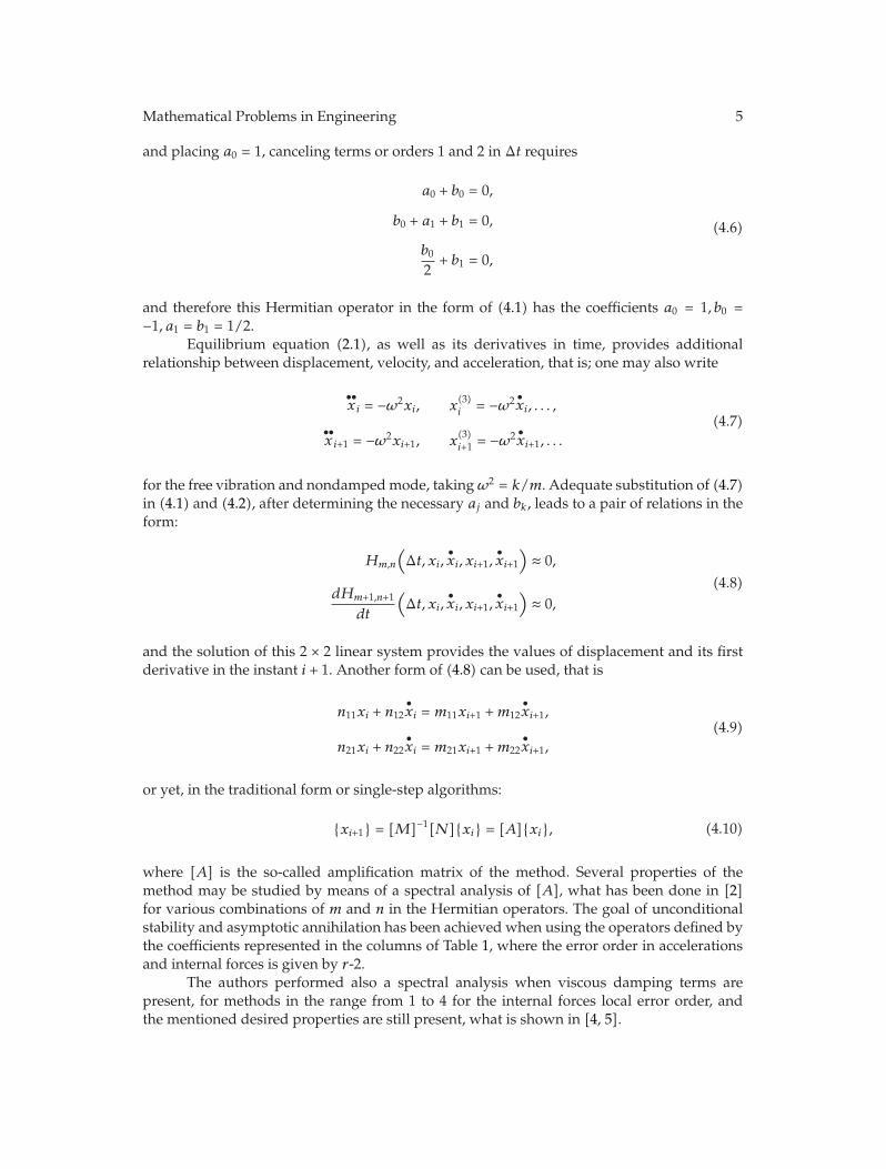
and placing a0 = 1, canceling terms or orders 1 and 2 in Δt requires

a0 + b0 = 0,

b0 + a1 + b1 = 0,

b0

2+ b1 = 0,

(4.6)

and therefore this Hermitian operator in the form of (4.1) has the coefficients a0 = 1, b0 =−1, a1 = b1 = 1/2.

Equilibrium equation (2.1), as well as its derivatives in time, provides additionalrelationship between displacement, velocity, and acceleration, that is; one may also write

••xi = −ω2xi, x

(3)i = −ω2 •xi, . . . ,

••xi+1 = −ω2xi+1, x

(3)i+1 = −ω2 •xi+1, . . .

(4.7)

for the free vibration and nondamped mode, takingω2 = k/m. Adequate substitution of (4.7)in (4.1) and (4.2), after determining the necessary aj and bk, leads to a pair of relations in theform:

Hm,n

(Δt, xi,

•xi, xi+1,

•xi+1

)≈ 0,

dHm+1,n+1

dt

(Δt, xi,

•xi, xi+1,

•xi+1

)≈ 0,

(4.8)

and the solution of this 2 × 2 linear system provides the values of displacement and its firstderivative in the instant i + 1. Another form of (4.8) can be used, that is

n11xi + n12•xi = m11xi+1 +m12

•xi+1,

n21xi + n22•xi = m21xi+1 +m22

•xi+1,

(4.9)

or yet, in the traditional form or single-step algorithms:

{xi+1} = [M]−1[N]{xi} = [A]{xi}, (4.10)

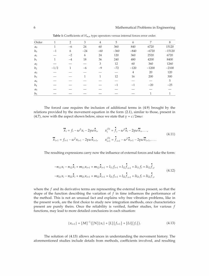
where [A] is the so-called amplification matrix of the method. Several properties of themethod may be studied by means of a spectral analysis of [A], what has been done in [2]for various combinations of m and n in the Hermitian operators. The goal of unconditionalstability and asymptotic annihilation has been achieved when using the operators defined bythe coefficients represented in the columns of Table 1, where the error order in accelerationsand internal forces is given by r-2.

The authors performed also a spectral analysis when viscous damping terms arepresent, for methods in the range from 1 to 4 for the internal forces local error order, andthe mentioned desired properties are still present, what is shown in [4, 5].


Table 1: Coefficients of Hm,n type operators versus internal forces error order.

Order 1 2 3 4 5 6 7 8a0 1 −6 24 60 360 840 6720 15120b0 −1 6 −24 −60 −360 −840 −6720 −15120a1 — −2 6 24 120 360 2520 6720b1 1 −4 18 36 240 480 4200 8400a2 — — — 3 12 60 360 1260b2 −1/2 1 −6 −9 −72 −120 −1200 −2100a3 — — — — — 4 20 120b3 — — 1 1 12 16 200 300a4 — — — — — — — 5b4 — — — — −1 −1 −20 −25a5 — — — — — — — —b5 — — — — — — 1 1

The forced case requires the inclusion of additional terms in (4.9) brought by therelations provided by the movement equation in the form (2.1), similar to those, present in(4.7), now with the aspect shown below, since we state that γ = c/2mω:

••xi = fi −ω2xi − 2γω

•xi, x

(3)i =

•fi −ω2 •xi − 2γω

••xi, . . . ,

••xi+1 = fi+1 −ω2xi+1 − 2γω

•xi+1, x

(3)i+1 =

•fi+1 −ω2 •xi+1 − 2γω

••xi+1, . . . .

(4.11)

The resulting expressions carry now the influence of external forces and take the form:

−n11xi − n12•xi +m11xi+1 +m12

•xi+1 = l11fi+1 + l12

•fi+1 + li11fi + li12

•fi,

−n21xi − n22•xi +m21xi+1 +m22

•xi+1 = l21fi+1 + l22

•fi+1 + li21fi + li22

•fi,

(4.12)

where the f and its derivative terms are representing the external forces present, so that theshape of the function describing the variation of f in time influences the performance ofthe method. This is not an unusual fact and explains why free vibration problems, like inthe present work, are the first choice to study new integration methods, once characteristicspresent are purely theirs. Once the reliability is verified, further studies, for various ffunctions, may lead to more detailed conclusions in each situation:

{xi+1} = [M]−1([N]{xi} + [L]{fi+1

}+ [Li]

{fi}). (4.13)

The solution of (4.13) allows advances in understanding the movement history. Theaforementioned studies include details from methods, coefficients involved, and resulting


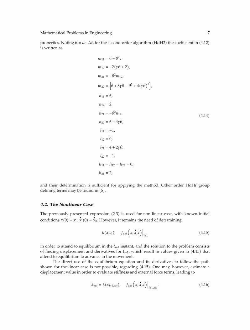
properties. Noting θ = ω ·Δt, for the second-order algorithm (HdH2) the coefficient in (4.12)is written as

m11 = 6 − θ2,

m12 = −2(γθ + 2

),

m21 = −θ2m12,

m22 =[6 + 8γθ − θ2 + 4

(γθ

)2],

n11 = 6,

n12 = 2,

n21 = −θ2n12,

n22 = 6 − 4γθ,

l11 = −1,

l12 = 0,

l21 = 4 + 2γθ,

l22 = −1,

li11 = li12 = li22 = 0,

li21 = 2,

(4.14)

and their determination is sufficient for applying the method. Other order HdHr groupdefining terms may be found in [5].

4.2. The Nonlinear Case

The previously presented expression (2.3) is used for non-linear case, with known initialconditions x(0) = x0,

•x (0) =

•x0. However, it remains the need of determining

k(xi+1), fext(x,•x, t

)∣∣∣i+1

(4.15)

in order to attend to equilibrium in the ti+1 instant, and the solution to the problem consistsof finding displacement and derivatives for ti+1, which result in values given in (4.15) thatattend to equilibrium to advance in the movement.

The direct use of the equilibrium equation and its derivatives to follow the pathshown for the linear case is not possible, regarding (4.15). One may, however, estimate adisplacement value in order to evaluate stiffness and external force terms, leading to

kest = k(xi+1,est), fext(x,•x, t

)∣∣∣i+1,est

. (4.16)


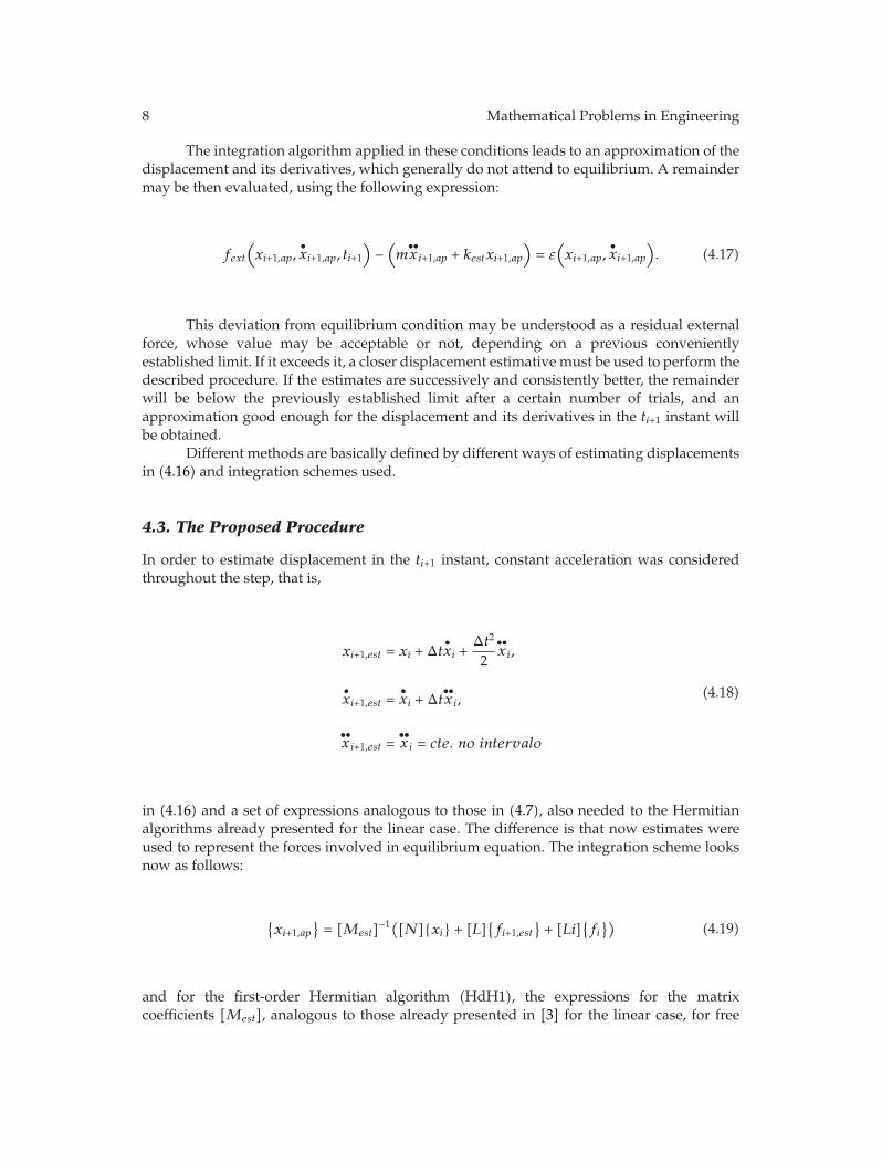
The integration algorithm applied in these conditions leads to an approximation of thedisplacement and its derivatives, which generally do not attend to equilibrium. A remaindermay be then evaluated, using the following expression:

fext(xi+1,ap,

•xi+1,ap, ti+1

)−(m••xi+1,ap + kestxi+1,ap

)= ε

(xi+1,ap,

•xi+1,ap

). (4.17)

This deviation from equilibrium condition may be understood as a residual externalforce, whose value may be acceptable or not, depending on a previous convenientlyestablished limit. If it exceeds it, a closer displacement estimative must be used to perform thedescribed procedure. If the estimates are successively and consistently better, the remainderwill be below the previously established limit after a certain number of trials, and anapproximation good enough for the displacement and its derivatives in the ti+1 instant willbe obtained.

Different methods are basically defined by different ways of estimating displacementsin (4.16) and integration schemes used.

4.3. The Proposed Procedure

In order to estimate displacement in the ti+1 instant, constant acceleration was consideredthroughout the step, that is,

xi+1,est = xi + Δt•xi +

Δt2

2••xi,

•xi+1,est =

•xi + Δt

••xi,

••xi+1,est =

••xi = cte. no intervalo

(4.18)

in (4.16) and a set of expressions analogous to those in (4.7), also needed to the Hermitianalgorithms already presented for the linear case. The difference is that now estimates wereused to represent the forces involved in equilibrium equation. The integration scheme looksnow as follows:

{xi+1,ap

}= [Mest]−1([N]{xi} + [L]

{fi+1,est

}+ [Li]

{fi})

(4.19)

and for the first-order Hermitian algorithm (HdH1), the expressions for the matrixcoefficients [Mest], analogous to those already presented in [3] for the linear case, for free


vibration and unitary mass, that is,

m11 = −1 +Δt2

2k(xi+1,est),

m12 = Δt,

m21 = −k(xi+1,est)Δt2

2,

m22 =

[k(xi+1,est)

Δt2

2− 1

]Δt,

(4.20)

while the [N] ones continue the same, already presented, taking the values shown below:

n11 = −1,

n12 = 0,

n21 = 0,

n22 = −Δt.

(4.21)

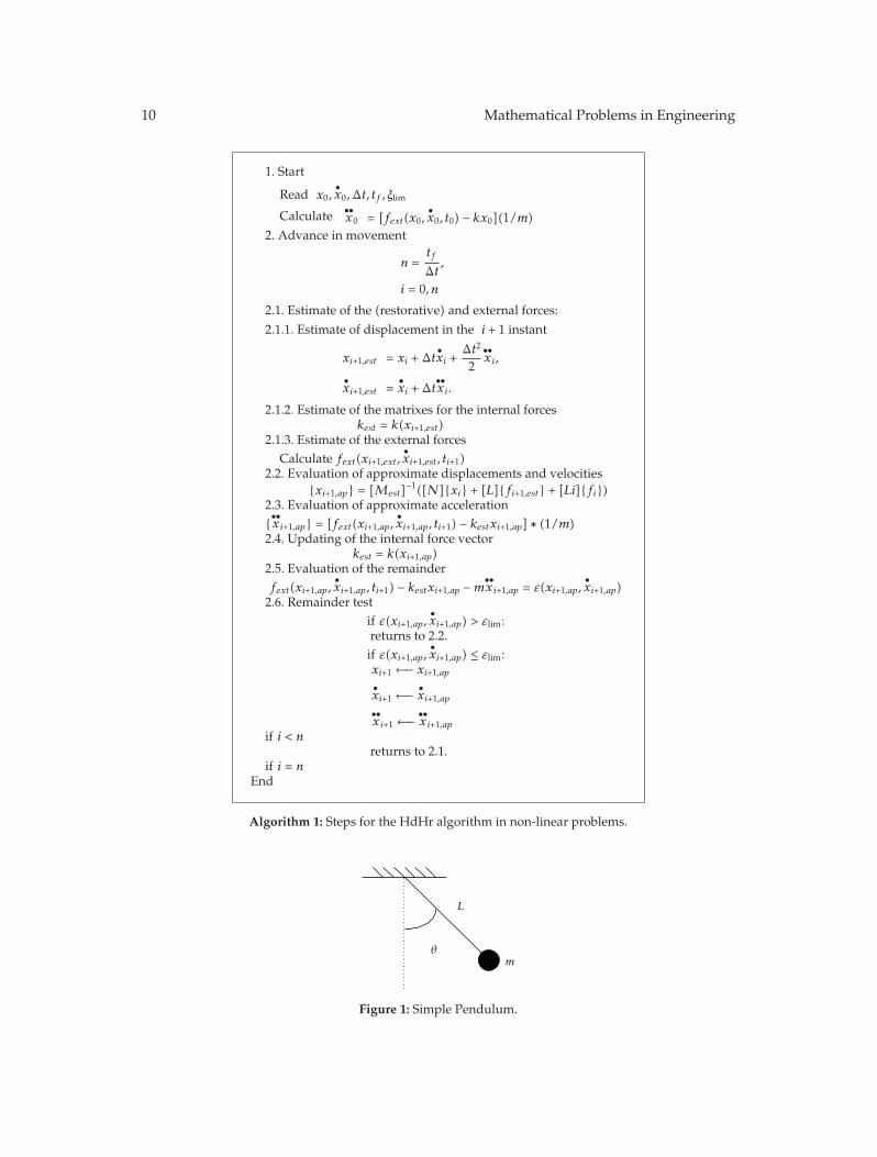
The coefficients of these matrixes for the other methods in this Hermitian group,with local error precision of second, third, and fourth orders (HdH2, HdH3, and HdH4),are obtained from those for the linear case, found in the already mentioned work. Once thesolution of (4.19) is at hand, the remainder can be calculated through (4.17). If it is lesser thana previously established limit, the approximate value for displacement and its derivatives isaccepted, and one advances in the movement history representation. If not, a new estimateof the matrixes in (4.16) is done to perform the integration scheme. The approximate valuesgiven by the solution of (4.19) are now used as new estimates and the procedure repeated.In other words, the system is solved again using the new estimates. This generates a newapproximation for displacement and velocity, a new remainder is calculated, its value isverified, and this procedure is continued until its limit is satisfied. The iterations for theconsidered step are then finalized, and one advances, initializing the procedure for the nextstep until the time interval of interest is completely covered. Algorithm 1 summarizes thesteps constituting the proposed procedure.

5. Example

The example shown is that of the simple pendulum, such as the addressed in [20]. Figure 1illustrates its scheme and notation used. It is a punctual mass m at the end of a rigid,weightless bar of length L, under gravity action, free to rotate around its other end. The angleof the bar in a given time is that measured positive to the right from a vertical line is θ.

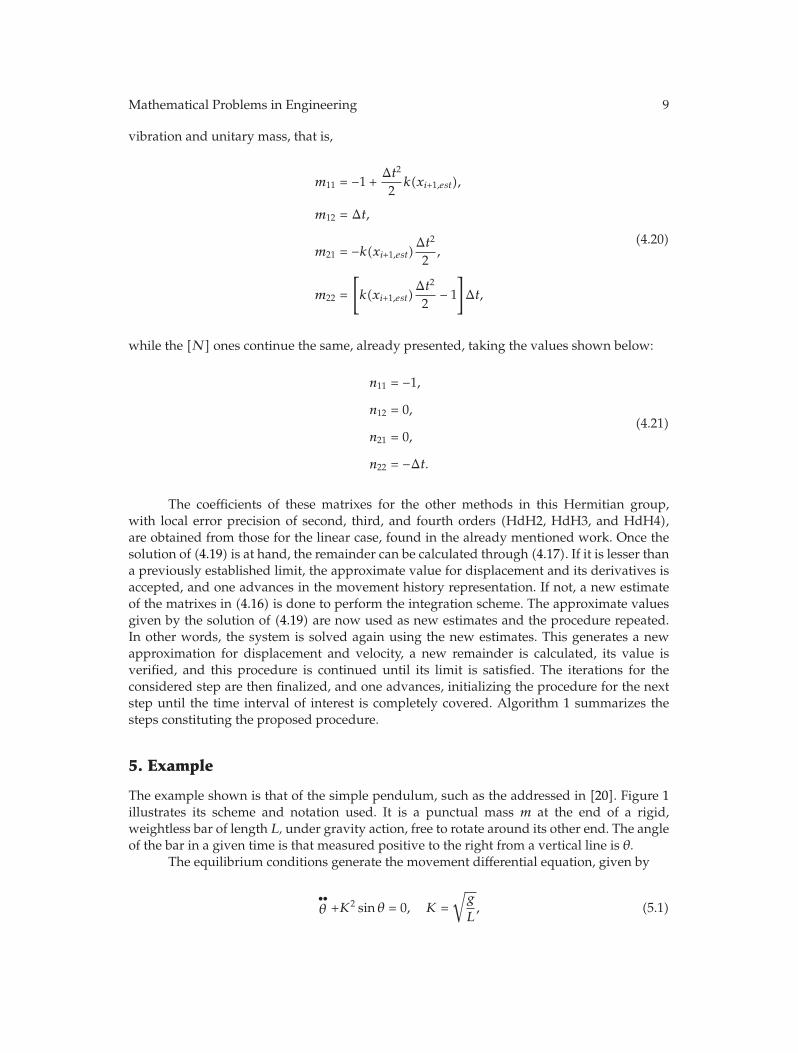
The equilibrium conditions generate the movement differential equation, given by

••θ +K2 sin θ = 0, K =

√g

L, (5.1)


1. Start

Read x0,•x0,Δt, tf , ξlim

Calculate ••x0 = [fext(x0,

•x0, t0) − kx0](1/m)

2. Advance in movement

n =tf

Δt,

i = 0, n

2.1. Estimate of the (restorative) and external forces:

2.1.1. Estimate of displacement in the i + 1 instant

xi+1,est = xi + Δt•xi +

Δt2

2••xi,

•xi+1,est =

•xi + Δt

••xi.

2.1.2. Estimate of the matrixes for the internal forceskest = k(xi+1,est)

2.1.3. Estimate of the external forcesCalculate fext(xi+1,ext,

•xi+1,est, ti+1)

2.2. Evaluation of approximate displacements and velocities{xi+1,ap} = [Mest]

−1([N]{xi} + [L]{fi+1,est} + [Li]{fi})2.3. Evaluation of approximate acceleration{••xi+1,ap} = [fext(xi+1,ap,

•xi+1,ap, ti+1) − kestxi+1,ap] ∗ (1/m)

2.4. Updating of the internal force vectorkest = k(xi+1,ap)

2.5. Evaluation of the remainderfext(xi+1,ap,

•xi+1,ap, ti+1) − kestxi+1,ap −m

••xi+1,ap = ε(xi+1,ap,

•xi+1,ap)

2.6. Remainder testif ε(xi+1,ap,

•xi+1,ap) > εlim:

returns to 2.2.if ε(xi+1,ap,

•xi+1,ap) ≤ εlim:

xi+1 ←− xi+1,ap

•xi+1 ←−

•xi+1,ap

••xi+1 ←−

••xi+1,ap

if i < nreturns to 2.1.

if i = nEnd

Algorithm 1: Steps for the HdHr algorithm in non-linear problems.

L

θm

Figure 1: Simple Pendulum.


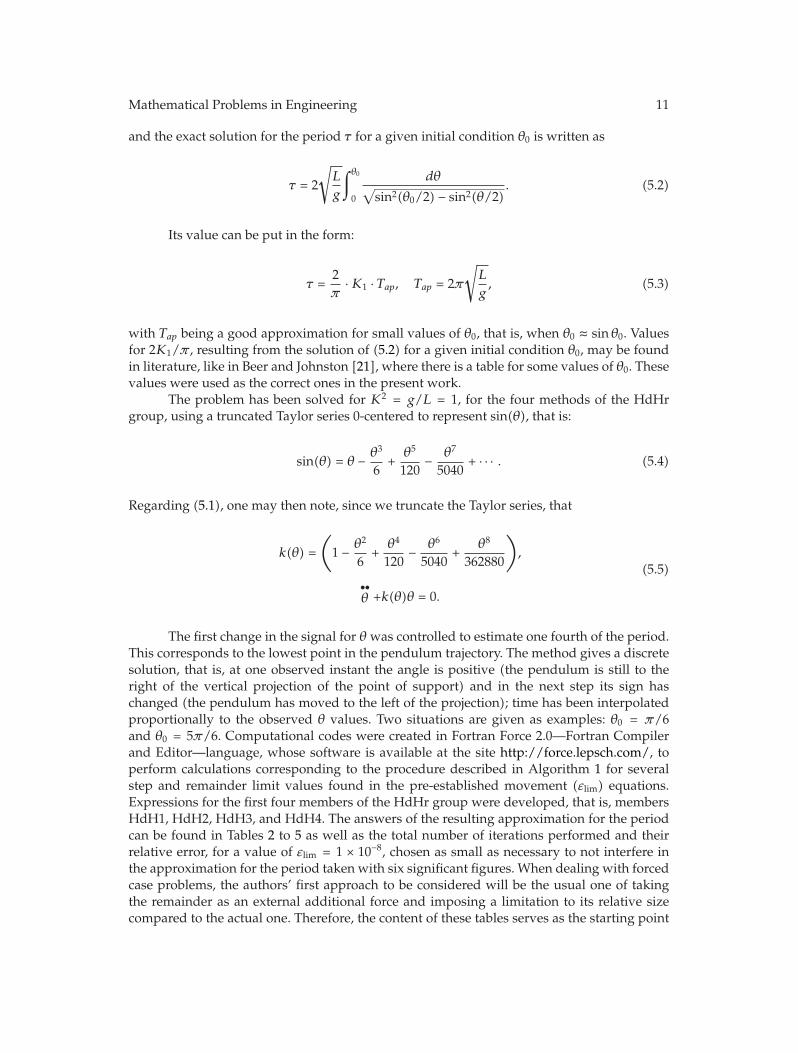
and the exact solution for the period τ for a given initial condition θ0 is written as

τ = 2

√L

g

∫θ0

0

dθ√sin2(θ0/2) − sin2(θ/2)

. (5.2)

Its value can be put in the form:

τ =2π·K1 · Tap, Tap = 2π

√L

g, (5.3)

with Tap being a good approximation for small values of θ0, that is, when θ0 ≈ sin θ0. Valuesfor 2K1/π , resulting from the solution of (5.2) for a given initial condition θ0, may be foundin literature, like in Beer and Johnston [21], where there is a table for some values of θ0. Thesevalues were used as the correct ones in the present work.

The problem has been solved for K2 = g/L = 1, for the four methods of the HdHrgroup, using a truncated Taylor series 0-centered to represent sin(θ), that is:

sin(θ) = θ − θ3

6+θ5

120− θ7

5040+ · · · . (5.4)

Regarding (5.1), one may then note, since we truncate the Taylor series, that

k(θ) =

(1 − θ

2

6+θ4

120− θ6

5040+

θ8

362880

),

••θ +k(θ)θ = 0.

(5.5)

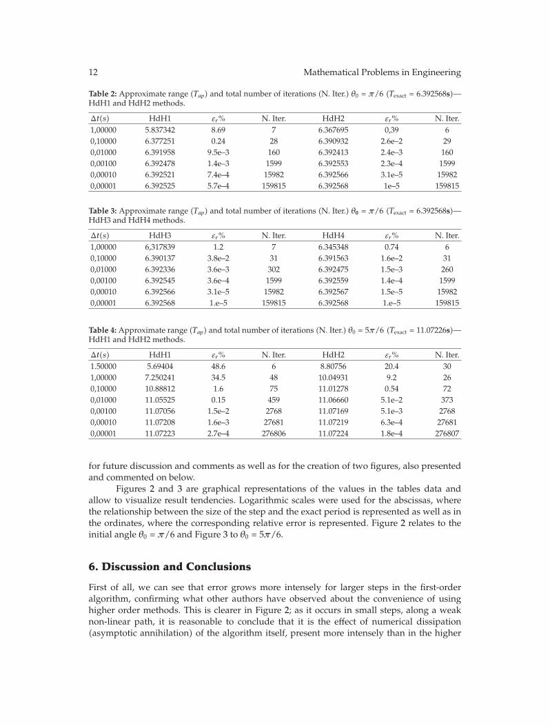
The first change in the signal for θ was controlled to estimate one fourth of the period.This corresponds to the lowest point in the pendulum trajectory. The method gives a discretesolution, that is, at one observed instant the angle is positive (the pendulum is still to theright of the vertical projection of the point of support) and in the next step its sign haschanged (the pendulum has moved to the left of the projection); time has been interpolatedproportionally to the observed θ values. Two situations are given as examples: θ0 = π/6and θ0 = 5π/6. Computational codes were created in Fortran Force 2.0—Fortran Compilerand Editor—language, whose software is available at the site http://force.lepsch.com/, toperform calculations corresponding to the procedure described in Algorithm 1 for severalstep and remainder limit values found in the pre-established movement (εlim) equations.Expressions for the first four members of the HdHr group were developed, that is, membersHdH1, HdH2, HdH3, and HdH4. The answers of the resulting approximation for the periodcan be found in Tables 2 to 5 as well as the total number of iterations performed and theirrelative error, for a value of εlim = 1 × 10−8, chosen as small as necessary to not interfere inthe approximation for the period taken with six significant figures. When dealing with forcedcase problems, the authors’ first approach to be considered will be the usual one of takingthe remainder as an external additional force and imposing a limitation to its relative sizecompared to the actual one. Therefore, the content of these tables serves as the starting point


Table 2: Approximate range (Tap) and total number of iterations (N. Iter.) θ0 = π/6 (Texact = 6.392568s)—HdH1 and HdH2 methods.

Δt(s) HdH1 εr% N. Iter. HdH2 εr% N. Iter.1,00000 5.837342 8.69 7 6.367695 0,39 60,10000 6.377251 0.24 28 6.390932 2.6e–2 290,01000 6.391958 9.5e–3 160 6.392413 2.4e–3 1600,00100 6.392478 1.4e–3 1599 6.392553 2.3e–4 15990,00010 6.392521 7.4e–4 15982 6.392566 3.1e–5 159820,00001 6.392525 5.7e–4 159815 6.392568 1e–5 159815

Table 3: Approximate range (Tap) and total number of iterations (N. Iter.) θ0 = π/6 (Texact = 6.392568s)—HdH3 and HdH4 methods.

Δt(s) HdH3 εr% N. Iter. HdH4 εr% N. Iter.1,00000 6,317839 1.2 7 6.345348 0.74 60,10000 6.390137 3.8e–2 31 6.391563 1.6e–2 310,01000 6.392336 3.6e–3 302 6.392475 1.5e–3 2600,00100 6.392545 3.6e–4 1599 6.392559 1.4e–4 15990,00010 6.392566 3.1e–5 15982 6.392567 1.5e–5 159820,00001 6.392568 1.e–5 159815 6.392568 1.e–5 159815

Table 4: Approximate range (Tap) and total number of iterations (N. Iter.) θ0 = 5π/6 (Texact = 11.07226s)—HdH1 and HdH2 methods.

Δt(s) HdH1 εr% N. Iter. HdH2 εr% N. Iter.1.50000 5.69404 48.6 6 8.80756 20.4 301,00000 7.250241 34.5 48 10.04931 9.2 260,10000 10.88812 1.6 75 11.01278 0.54 720,01000 11.05525 0.15 459 11.06660 5.1e–2 3730,00100 11.07056 1.5e–2 2768 11.07169 5.1e–3 27680,00010 11.07208 1.6e–3 27681 11.07219 6.3e–4 276810,00001 11.07223 2.7e–4 276806 11.07224 1.8e–4 276807

for future discussion and comments as well as for the creation of two figures, also presentedand commented on below.

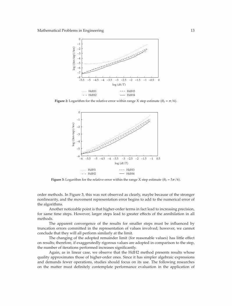
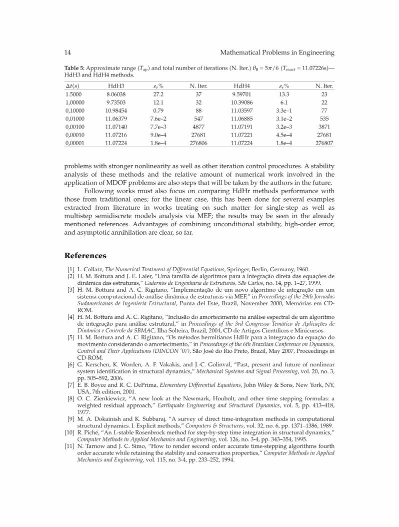
Figures 2 and 3 are graphical representations of the values in the tables data andallow to visualize result tendencies. Logarithmic scales were used for the abscissas, wherethe relationship between the size of the step and the exact period is represented as well as inthe ordinates, where the corresponding relative error is represented. Figure 2 relates to theinitial angle θ0 = π/6 and Figure 3 to θ0 = 5π/6.

6. Discussion and Conclusions

First of all, we can see that error grows more intensely for larger steps in the first-orderalgorithm, confirming what other authors have observed about the convenience of usinghigher order methods. This is clearer in Figure 2; as it occurs in small steps, along a weaknon-linear path, it is reasonable to conclude that it is the effect of numerical dissipation(asymptotic annihilation) of the algorithm itself, present more intensely than in the higher


−8

−7

−6

−5

−4

−3

−2

−1

0

log((

tex-

tap)

/te

x)

−5.5 −5 −4.5 −4 −3.5 −3 −2.5 −2 −1.5 −1 −0.5 0

log (dt/T)

HdH1HdH2

HdH3HdH4

Figure 2: Logarithm for the relative error within range X step estimate (θ0 = π/6).

−6

−5

−4

−3

−2

−1

0

log((

tex-

tap)

/te

x)

−6 −5.5 −5 −4.5 −4 −3.5 −3 −2.5 −2 −1.5 −1 0.5

log (dt/T)

HdH1HdH2

HdH3HdH4

Figure 3: Logarithm for the relative error within the range X step estimate (θ0 = 5π/6).

order methods. In Figure 3, this was not observed as clearly, maybe because of the strongernonlinearity, and the movement representation error begins to add to the numerical error ofthe algorithms.

Another noticeable point is that higher-order terms in fact lead to increasing precision,for same time steps. However, larger steps lead to greater effects of the annihilation in allmethods.

The apparent convergence of the results for smaller steps must be influenced bytruncation errors committed in the representation of values involved; however, we cannotconclude that they will all perform similarly at the limit.

The changing of the adopted remainder limit (for reasonable values) has little effecton results; therefore, if exaggeratedly rigorous values are adopted in comparison to the step,the number of iterations performed increases significantly.

Again, as in linear case, we observe that the HdH2 method presents results whosequality approximates those of higher-order ones. Since it has simpler algebraic expressionsand demands fewer operations, studies should focus on its use. The following researcheson the matter must definitely contemplate performance evaluation in the application of


Table 5: Approximate range (Tap) and total number of iterations (N. Iter.) θ0 = 5π/6 (Texact = 11.07226s)—HdH3 and HdH4 methods.

Δt(s) HdH3 εr% N. Iter. HdH4 εr% N. Iter.1.5000 8.06038 27.2 37 9.59701 13.3 231,00000 9.73503 12.1 32 10.39086 6.1 220,10000 10.98454 0.79 88 11.03597 3.3e–1 770,01000 11.06379 7.6e–2 547 11.06885 3.1e–2 5350,00100 11.07140 7.7e–3 4877 11.07191 3.2e–3 38710,00010 11.07216 9.0e–4 27681 11.07221 4.5e–4 276810,00001 11.07224 1.8e–4 276806 11.07224 1.8e–4 276807

problems with stronger nonlinearity as well as other iteration control procedures. A stabilityanalysis of these methods and the relative amount of numerical work involved in theapplication of MDOF problems are also steps that will be taken by the authors in the future.

Following works must also focus on comparing HdHr methods performance withthose from traditional ones; for the linear case, this has been done for several examplesextracted from literature in works treating on such matter for single-step as well asmultistep semidiscrete models analysis via MEF; the results may be seen in the alreadymentioned references. Advantages of combining unconditional stability, high-order error,and asymptotic annihilation are clear, so far.

References

[1] L. Collatz, The Numerical Treatment of Differential Equations, Springer, Berlin, Germany, 1960.[2] H. M. Bottura and J. E. Laier, “Uma famılia de algoritmos para a integracao direta das equacoes de

dinamica das estruturas,” Cadernos de Engenharia de Estruturas, Sao Carlos, no. 14, pp. 1–27, 1999.[3] H. M. Bottura and A. C. Rigitano, “Implementacao de um novo algoritmo de integracao em um

sistema computacional de analise dinamica de estruturas via MEF,” in Proceedings of the 29th JornadasSudamericanas de Ingenierıa Estructural, Punta del Este, Brazil, November 2000, Memorias em CD-ROM.

[4] H. M. Bottura and A. C. Rigitano, “Inclusao do amortecimento na analise espectral de um algoritmode integracao para analise estrutural,” in Proceedings of the 3rd Congresso Tematico de Aplicacoes deDinamica e Controle da SBMAC, Ilha Solteira, Brazil, 2004, CD de Artigos Cientıficos e Minicursos.

[5] H. M. Bottura and A. C. Rigitano, “Os metodos hermitianos HdHr para a integracao da equacao domovimento considerando o amortecimento,” in Proceedings of the 6th Brazilian Conference on Dynamics,Control and Their Applications (DINCON ’07), Sao Jose do Rio Preto, Brazil, May 2007, Proceedings inCD-ROM.

[6] G. Kerschen, K. Worden, A. F. Vakakis, and J.-C. Golinval, “Past, present and future of nonlinearsystem identification in structural dynamics,” Mechanical Systems and Signal Processing, vol. 20, no. 3,pp. 505–592, 2006.

[7] E. B. Boyce and R. C. DePrima, Elementary Differential Equations, John Wiley & Sons, New York, NY,USA, 7th edition, 2001.

[8] O. C. Zienkiewicz, “A new look at the Newmark, Houbolt, and other time stepping formulas: aweighted residual approach,” Earthquake Engineering and Structural Dynamics, vol. 5, pp. 413–418,1977.

[9] M. A. Dokainish and K. Subbaraj, “A survey of direct time-integration methods in computationalstructural dynamics. I. Explicit methods,” Computers & Structures, vol. 32, no. 6, pp. 1371–1386, 1989.

[10] R. Piche, “An L-stable Rosenbrock method for step-by-step time integration in structural dynamics,”Computer Methods in Applied Mechanics and Engineering, vol. 126, no. 3-4, pp. 343–354, 1995.

[11] N. Tarnow and J. C. Simo, “How to render second order accurate time-stepping algorithms fourthorder accurate while retaining the stability and conservation properties,” Computer Methods in AppliedMechanics and Engineering, vol. 115, no. 3-4, pp. 233–252, 1994.


[12] P. Nawrotzki and C. Eller, “Numerical stability analysis in structural dynamics,” Computer Methods inApplied Mechanics and Engineering, vol. 189, no. 3, pp. 915–929, 2000.

[13] F. Armero and I. Romero, “On the formulation of high-frequency dissipative time-steppingalgorithms for nonlinear dynamics. I. Low-order methods for two model problems and nonlinearelastodynamics,” Computer Methods in Applied Mechanics and Engineering, vol. 190, no. 20-21, pp. 2603–2649, 2001.

[14] F. Armero and I. Romero, “On the formulation of high-frequency dissipative time-steppingalgorithms for nonlinear dynamics. II. Second-order methods,” ComputerMethods in AppliedMechanicsand Engineering, vol. 190, no. 51-52, pp. 6783–6824, 2001.

[15] A. Bonelli, O. S. Bursi, and M. Mancuso, “Explicit predictor-multicorrector time discontinuousGalerkin methods for non-linear dynamics,” Journal of Sound and Vibration, vol. 256, no. 4, pp. 695–724,2002.

[16] S. Modak and E. D. Sotelino, “The generalized method for structural dynamics applications,”Advances in Engineering Software, vol. 33, no. 7–10, pp. 565–575, 2002.

[17] M. Mancuso and F. Ubertini, “An efficient time discontinuous Galerkin procedure for non-linearstructural dynamics,” Computer Methods in Applied Mechanics and Engineering, vol. 195, no. 44–47, pp.6391–6406, 2006.

[18] H. M. Hilber and T. J. R. Hughes, “Collocation, dissipation and overshoot for time integration schemesin structural dynamics,” Earthquake Engineering and Structural Dynamics, vol. 6, pp. 99–117, 1978.

[19] P. Hauret and P. Le Tallec, “Energy-controlling time integration methods for nonlinear elastodynamicsand low-velocity impact,” Computer Methods in Applied Mechanics and Engineering, vol. 195, no. 37–40,pp. 4890–4916, 2006.

[20] T. Pacitti and C. P. Atkinson, Programacao e Metodos Computacionais, Livros Tecnicos e CientıficosEditora S. A., Rio de Janeiro, Brazil, 2nd edition, 1977.

[21] F. P. Beer and E. R. Johnston Jr., Mecanica Vetorial para Engenheiros, vol. 2, McGraw-Hill do Brasil, SaoPaulo, Brazil, 1976.

About the Use of the HdHr Algorithm Group in Integrating ... · Heitor Miranda Bottura and Antonio...

Documents

Transcript of About the Use of the HdHr Algorithm Group in Integrating ... · Heitor Miranda Bottura and Antonio...