About Clapeyron’s Theorem in Linear Elasticity · ABOUT CLAPEYRON’S THEOREM 147 where n is the...

Journal of Elasticity 72: 145–172, 2003.© 2003 Kluwer Academic Publishers. Printed in the Netherlands.

145

About Clapeyron’s Theorem in Linear Elasticity �

ROGER FOSDICK and LEV TRUSKINOVSKYDepartment of Aerospace Engineering and Mechanics, University of Minnesota, Minneapolis,MN 55455, U.S.A. E-mail: [email protected], [email protected]

Received: 6 August 2002; in revised form: 17 March 2003

Abstract. We examine some elementary interpretations of the classical theorem of CLAPEYRON

in linear elasticity theory. As we show, a straightforward application of this theorem in the purelymechanical setting leads to an apparent paradox which can be resolved by referring either to dynam-ics or to thermodynamics. These richer theories play an essential part in understanding the physicalsignificance of this theorem.

Mathematics Subject Classifications (2000): 74A15, 74B05, 80A17

Key words: elasticity, Clapeyron, dissipation, viscoelasticity, thermoelasticity.

In remembrance of Clifford Truesdell and his scientific program of enlightenment.

1. Introduction

According to Love [11, p. 173], “The potential energy of deformation of a body,which is in equilibrium under given load, is equal to half the work done by theexternal forces, acting through the displacements from the unstressed state to thestate of equilibrium.” This is now commonly known as CLAPEYRON’s theoremin linear elasticity theory.�� In particular, this theorem, taken literally, implies thatthe elastic stored energy accounts for only half of the energy spent to load thebody; the remaining half of the work done to the body by the external forces isunaccounted for and is lost somewhere in achieving the equilibrium state. It isparticularly striking that this apparent paradox is reached within the framework of

� The National Science Foundation Grant No. DMS-0102841 is gratefully acknowledged for theirsupport of this research.�� In 1852, Lame [9] published his volume, Leçons sur la theorie mathematique de l’elasticite des

corps solides, in which he devoted his seventh lecture to what he termed CLAPEYRON’s Theorem.(See [13, pp. 565 and 578], for relevant remarks.) Earlier, Lame and Clapeyron [10] had noted thisresult in a joint memoir of 1833. Although Emile Clapeyron [3], himself, first published on thistheorem in 1858, in a resume of an original memoir that apparently was never published, it is arguedby Todhunter and Pearson [14, p. 419], that the “result of the memoir of 1833 was due entirely toClapeyron, for Lame in his Leçons, of 1852, . . . terms it CLAPEYRON’s Theorem, and CLAPEYRON

here speaks of it as he would do only if it were entirely due to himself.”

146 R. FOSDICK AND L. TRUSKINOVSKY

the purely conservative linear theory of elasticity. Alternatively, however, withinelastostatics the common characterization of the work done to reach equilibrium isconceptually ambiguous and a different interpretation may be required.

To illustrate the above concerns, let us first recall that in the linear theory ofelasticity the total strain energy of a body that occupies the region � ⊂ R

3 andsupports a, generally, dynamical displacement field u = u(x, t) and strain fielde ≡ (∇u + (∇u)T)/2 = e(x, t) relative to its undistorted state at time t = 0 isdefined by

U [e](t) ≡∫�

1

2ρC[e] · e dv. (1.1)

Here, ρ is the mass density of the body and C is the positive definite and completelysymmetric elasticity tensor. Further, the work done during the interval of time (0, t)due to an applied boundary traction field t∗ = t∗(x, t) and body force field b∗ =b∗(x, t) over the displacement u(x, t) is given by

W [u](t) =∫ t

0

(∫∂�

t∗ · u da +∫�

b∗ · u dv

)dt. (1.2)

The corresponding stress field in � at time t , T = T(x, t), satisfies the generalizedHOOKE’S law T = ρC[e] and is symmetric. Throughout this paper we shall as-sume, for convenience, that the body is homogeneous, so that ρ and C are constant.If the loads t∗ and b∗ are ‘dead’, i.e., independent of time, so that t∗ = t(x) andb∗ = b(x), then for a body that is undistorted at time t = 0, (1.2) may be integratedto yield

W [u](t)|(t∗,b∗)=(t,b) =∫∂�

t · u da +∫�

b · u dv ≡ W [u](t). (1.3)

This ‘dead load work’ represents the “work done by the external forces” to whichLOVE referred in his quote concerning equilibrium reproduced in the first line ofthis introduction, above. Of course, in this case the loads are equilibrated so that∫

∂�

t da +∫�

b dv = 0,∫∂�

x × t da +∫�

x × b dv = 0 (1.4)

and u is an equilibrium displacement field, say u(x); the corresponding ‘dead loadwork’ is then

W [u] ≡ W [u](t)|u=u(x). (1.5)

Suppose that the displacement field u = u(x) corresponds to an equilibriumstate with strain e(x) and stress T(x) satisfying T = ρC[e] and

div T + b = 0 in �, Tn = t on ∂�, (1.6)

ABOUT CLAPEYRON’S THEOREM 147

where n is the outer unit normal to � on ∂�. Without loss of generality, we mayeliminate the possibility of an added infinitesimal rigid displacement field in u(x)and render u(x) unique by imposing the normalization conditions∫

�

ρu dv = 0,∫�

ρx × u dv = 0, (1.7)

where the mass density ρ is included only for later convenience. Then, according tothe usual derivation of CLAPEYRON’s theorem, we see, starting with (1.3) and (1.5)and using (1.6), generalized HOOKE’S law, the symmetry of T and the divergencetheorem, that

1

2W [u] = 1

2

(∫∂�

Tn · u da +∫�

b · u dv

)= U [e]. (1.8)

Literally following LOVE’s statement of CLAPEYRON’s theorem, one may inferthat elastostatics alone� accounts for only half of the work that is expended toreach equilibrium; the coefficient one-half is a result of the linearity of the the-ory. In the remainder of this paper, we continue within the linear framework andconsider, respectively, in Sections 2, 3 and 4, the richer dynamical theories of elas-ticity, viscoelasticity and thermoelasticity in order to shed light on this seeminglyparadoxical and incomplete conclusion.

SYNOPSIS

In Section 2, we argue that within ideal elasticity theory the quantity W [u] ofCLAPEYRON’s theorem does not reasonably represent the work done by the exter-nal forces to reach an elastostatic equilibrium state u = u(x). We then investigate‘fast’ versus ‘slow’ time dependent loading conditions and conclude that within theassumptions of elastostaticsW [u]/2 is a better representative of the work expendedto reach equilibrium. In Sections 3 and 4, we amend ideal elasticity theory so asto include the mechanisms of viscous and thermal dissipation, respectively. Thendead loading becomes compatible with the notion of achieving equilibrium and,we conclude that the quantity W [u] of CLAPEYRON’s theorem does adequatelyrepresent the corresponding work done by the external applied forces. Here wefind that half ofW [u] becomes stored in the body in the form of equilibrium strainenergy and the remaining half is dissipated either through the action of viscousdissipation or heat transfer. In Section 5, we offer some conclusions.

� In elastostatics, there is, of course, no time dependence and formally the work done by the loadst(x) and b(x) to reach the equilibrium displacement u = u(x) from an undistorted state commonlyis calculated by using (1.3) and (1.5), as was done in (1.8). As noted earlier, for purely equilibriumtheory this may not properly represent the ‘work done to reach equilibrium’ because this tacitlyassumes that the loads are ‘dead’ and applied over time and, therefore, impulsive. For an ideal elasticbody this circumstance is not compatible with the notion of reaching equilibrium, as we shall see inSection 2 and related Appendices A and B.


In Appendices A and B, we show some example calculations to further illus-trate the claims of Section 2. It should be noted that throughout the main body ofthis paper we assume, for convenience, that the traction field is specified on thecomplete boundary of �. However, in the elementary examples of these appen-dices we prefer to hold one part of the boundary fixed and specify the traction onthe complementary part for all time. While these boundary conditions clearly arenot consistent with (1.4)1 and (2.4)1, nevertheless they are normal and allowable;moreover, they do not compromise the main purpose of illustrating the differencebetween dead and retarded loading.

2. Elastodynamics

Here, we shall first consider the consequences of ‘dead’ loading within elastody-namics regarding work and energy and then show how equilibrium theory is bestaccounted for by introducing a retarded system of loads.

2.1. ‘DEAD’ LOADING

Suppose that for all time t > 0 the body is ‘dead’ loaded with the same loads as inthe static situation described above, so that t∗ = t(x) and b∗ = b(x) in (1.2). Onthe boundary of � we set

Tn = t on ∂�, ∀t > 0, (2.1)

and initially the body is at rest and undistorted so that

u(x, 0) = u(x, 0) = 0 in �. (2.2)

The dynamical equation is

div T + b = ρu in �, ∀t > 0, (2.3)

and we recall that t = t(x) and b = b(x) are supposed to be balanced in thesense of (1.4). Of course, u, e and T are related through the strain-displacementand stress–strain equations of Section 1. Under these conditions, it readily follows,from (2.1), (2.3) and the symmetry of T, that the linear and angular momentum areconserved. Thus, by integration in time and use of (2.2), it is clear that the resultingmotion naturally satisfies the normalization∫

�

ρu dv = 0,∫�

ρx × u dv = 0 ∀t � 0. (2.4)

In addition, by forming the inner product of (2.3) with u, integrating over� and us-ing the symmetry of C together with (2.1) and (1.1), we readily reach the classicalpower theorem∫

∂�

t · u da +∫�

b · u dv = d

dtU [e](t)+ d

dtK[u](t), (2.5)


where

K[u](t) ≡∫�

1

2ρ|u|2 dv (2.6)

is the kinetic energy of the body. Then, by integrating (2.5) in time and using (2.2)and (1.3) we obtain the standard balance of mechanical energy

W [u](t) = U [e](t)+K[u](t), (2.7)

which is supposed to be valid for all time t � 0.Now, as a first elementary observation, let us assume that � may, at some time

t = t during the motion, instantaneously support the equilibrium displacement fieldin the sense that u(x, t ) = u(x); it may be that u(·, t ) �= 0 so � is not coincidentlyat rest. Be that as it may, nevertheless, (2.4) will be met at t = t because of (1.7)and, in addition, because W [u](t ) = W [u] and U [e](t ) = U [e], we see from (2.7)that

W [u] = U [e] +K[u](t). (2.8)

Then, recalling (1.8), we may conclude that half the work done during the timeinterval (0, t ) is stored in the body as strain energy and the remaining half satisfies

1

2W [u] = K[u](t ); (2.9)

it has been spent to produce the instantaneous kinetic energy of the body. Ac-cordingly, under the present circumstances, it is this kinetic energy that must bespontaneously extracted from � if the body is to be arrested in the equilibriumstate u(x, t ) = u(x). However, there is no mechanism in this conservative idealelastic system to do so!�

Let us now consider an alternative description of how the work may be chan-neled into strain energy and kinetic energy based upon time-averaging of the corre-sponding energies. The assumption here is that there is a time t = t∗ > 0, perhapsone among many, at which the body instantaneously is at rest, i.e., u(x, t∗) ≡ 0in �.�� To describe the average motion, we introduce the time-average displace-ment field as

〈u〉(x) ≡ 1

t∗

∫ t∗

0u(x, t) dt, (2.10)

� According to [11, p. 123] (see also [13, p. 537, art. 988]), in 1839 Poncelet [12] was thefirst to note that “a load suddenly applied may cause a strain twice as great as that produced bya gradual application of the same load.” While this observation of Poncelet, which also containsan interesting factor of 2, appeared contemporaneously with the original and later announcements ofCLAPEYRON’s theorem, there appears to have been no recognition of a possible relationship betweenthe claims of either authors.�� While, generally, there may not be such a time, in the case of periodic motion there is a countable

set of such times; a specific one-dimensional example is discussed later in Appendix A. Notice,though, that according to (2.4)1 the average of u(x, t) over � is always zero.


with the time-average strain 〈e〉(x) and stress 〈T〉(x) fields defined analogously.Then, it readily follows that

〈e〉 = 1

2

(∇〈u〉 + (∇〈u〉)T), 〈T〉 = ρC[〈e〉]. (2.11)

Moreover, because of (2.2), by time-averaging (2.3) and (2.1) we find

div〈T〉 + b = 0 in �, 〈T〉n = t on ∂�. (2.12)

Also, note that the time-average displacement field 〈u〉(x) satisfies the normaliza-tion (2.4) and recall that the loads t = t(x) and b = b(x) are balanced in the senseof (1.4). Thus, because of uniqueness and the fact that 〈u〉(x) and u(x) solve thesame equilibrium boundary-value problem, we may conclude that

〈u〉(x) = u(x), 〈e〉(x) = e(x), 〈T〉(x) = T(x) in �. (2.13)

Now, by time-averaging (2.7), using (1.3), recalling the notation establishedin (2.10) and applying (2.13), we easily have

〈W [u]〉 = W [〈u〉] = W [u] = 〈U [e]〉 + 〈K[u]〉. (2.14)

In particular, the average of the ‘dead load work’, 〈W [u]〉, is equal to the quantityW [u] of CLAPEYRON’s theorem in (1.8), and our immediate aim is to determinehow this average work expended is divided up between the average strain energy〈U [e]〉 and the average kinetic energy 〈K[u]〉 of the body. To do so, we firstintroduce the difference displacement field

u′(x, t) ≡ u(x, t)− u(x), (2.15)

with e′(x, t) and T′(x, t) defined analogously, and observe, using (1.1), the sym-metry of C and (1.8), that

U [e](t) =∫�

1

2ρC[e + e′] · (e + e′) dv

= U [e] +∫�

ρC[e] · e′ dv + U [e′](t)

= 1

2W [u] +

∫�

ρC[e] · e′ dv + U [e′](t).

Then, by time-averaging we have

〈U [e]〉 = 1

2W [u] +

∫�

ρC[e] · 〈e′〉 dv + 〈U [e′]〉.

However, because e′(x, t) = e(x, t) − e(x) we see from (2.13) that 〈e′〉(x) =〈e〉(x)− e(x) = 0 and, consequently, we reach

〈U [e]〉 = 1

2W [u] + 〈U [e′]〉. (2.16)


Now, to determine 〈U [e′]〉, it is convenient to observe, using (2.1)–(2.3), (2.15)and the relationships T′ = ρC[e′] and e′ = (∇u′ + (∇u′)T)/2, that

div T′ = ρu′ in �, ∀t > 0,(2.17)

T′n = 0 on ∂�, ∀t > 0; u′(x, 0) = −u(x), u′(x, 0) = 0 in �.

Then, with the definition (1.1), the symmetry of C, (2.17) and the aid of the diver-gence theorem we find that

U [e′](t) = 1

2

∫�

T′ · ∇u′ dv

= 1

2

∫∂�

T′n · u′ da − 1

2

∫�

ρu′ · u′ dv

= −1

2

∫�

ρu′ · u′ dv

= −1

2

∫�

( ˙ρu · u′ − ρ|u|2

)dv,

the last equation of which uses the fact that (2.15) implies u′(x, t) = u(x, t). Now,by time-averaging, recalling that u(x, 0) = u(x, t∗) = 0 and using (2.6), we obtain

〈U [e′]〉 = 〈K[u]〉, (2.18)

which is a well known result concerning the equipartition between kinetic andpotential energies. Thus, by substituting (2.18) into (2.16) and then using (2.14)we conclude that

〈U [e′]〉 = 〈K[u]〉 = 1

4W [u] (2.19)

and, again using (2.16), we see that

〈U [e]〉 = 1

2W [u] + 1

4W [u] = 3

4W [u]. (2.20)

To show that this result is independent of the assumption of periodicity, let us in-troduce the complete set of orthonormal eigenfunctions and eigenvalues, {ui(x), ωi,i = 1, 2, . . .}, which satisfy (1.7) and

div(C[∇ui])+ ρω2i ui = 0 in �,

(2.21)(C[∇ui])n = 0 on ∂�,

and expand the solution u(x, t) of (2.1)–(2.3) in the form

u(x, t) =∞∑i=1

ui(x)gi(t).


Then, we readily find that gi(t) = Ai(1 − cosωit), i = 1, 2, . . . , and it is possibleto determine the constants Ai as Fourier coefficients so that this series representsa weak solution of (2.1)–(2.3) in the sense that ∇u(·, t) ∈ L2(�) for all t > 0.Furthermore, it is straightforward to show that the infinite time-average of thedisplacement field,

〈u〉∞(x) ≡ limT→∞

1

T

∫ T

0u(x, t) dt, (2.22)

satisfies 〈u〉∞(x) = u(x) and that conclusions similar to those highlighted in theprevious paragraph continue to hold for the relationships between the infinite time-averages of the work, strain energy and kinetic energy, i.e.,

〈W [u]〉∞ = W [〈u〉∞] = W [u] = 〈U [e]〉∞ + 〈K[u]〉∞ (2.23a)

with

〈U [e]〉∞ = 3

4W [u], 〈K[u]〉∞ = 1

4W [u]. (2.23b)

Based upon the above analyses, we conclude that when an elastic body is set inmotion with a ‘dead’ loading system from an initially undistorted rest state, then,with suitable interpretation, the average work that is supplied to the body by the‘dead’ loading is equal to the equilibrium work of CLAPEYRON’s theorem. Onthe average, three quarters of this work appears as strain energy (half due to theequilibrium strain energy as predicted from CLAPEYRON’s theorem and a quarterdue to the strain energy of the deformation relative to this equilibrium), and theremaining quarter is, on the average, transformed into kinetic energy.

To illustrate the general conclusions reached above, we consider, in Appen-dix A, a specific one-dimensional elastodynamic problem with ‘dead’ loading.

2.2. ‘SLOW’ LOADING

When an ideal elastic body is ‘dead’ loaded from an undistorted, rest state with anotherwise equilibrium system of loads, the loading is impulsively applied. Conse-quently, from the dynamical considerations of Section 2.1, the body never reachesequilibrium but, rather, rings by constantly redistributing kinetic and strain energybetween its elements. Indeed, the work done to the body at any time t > 0 dueto the external loading is given by (1.3), but the body is never coincidently at restand in a state of equilibrium. On the other hand, we expect that if an equilibriumsystem of loads is achieved sufficiently slowly in time then even an ideal elasticbody should distort through a sequence of near equilibrium states and eventuallyreach a nearly static equilibrium configuration. In this case, the work done to thebody at any time t due to the external loading may be calculated using (1.2), butthe calculation is no longer trivial because now t∗ and b∗ are not ‘dead’ but ratherdepend on time. For dissipationless, ideal elastic bodies it is intuitively clear that


the work expended to reach equilibrium should be related to the latter rather thanthe former calculation.

To gain some general perspective, suppose that the loading system, t∗ on ∂�and b∗ in �, is such that

t∗ = t∗(x, t) =t

t∞t(x), t ∈ (0, t∞),

t(x), t � t∞,(2.24)

and

b∗ = b∗(x, t) =t

t∞b(x), t ∈ (0, t∞),

b(x), t � t∞,(2.25)

where t∞ is a sufficiently large time constant so that the loads may be consideredto be slowly applied. Then, at least for t ∈ (0, t∞), the displacement field u =u(x, t) = t u(x)/t∞ and the corresponding strain and stress fields, e = e(x, t) =t e(x)/t∞ and T = T(x, t) = tT(x)/t∞, from the strain-displacement and stress–strain relations of Section 1, will satisfy the dynamical equation

div T + b∗ = ρu in �, t ∈ (0, t∞),together with the boundary condition

Tn = t∗ on ∂�, t ∈ (0, t∞)and initial conditions

u(x, 0) = 0, u(x, 0) = 1

t∞u(x) in �.

Clearly, for sufficiently large time constant t∞ not only is the applied loading‘slow’, but the initial state of � is undistorted and ‘nearly’ at rest. Further, at timet = t∞ the body achieves the equilibrium displacement field u(x) with, again,‘nearly’ zero velocity. Moreover, according to (1.2), the work done to� up to timet = t∞ is

W [u](t∞) =∫ t∞

0

(∫∂�

t

t∞t · 1

t∞u da +

∫�

t

t∞b · 1

t∞u dv

)dt

= 1

2

(∫∂�

t · u da +∫�

b · u dv

),

so that with (1.8)1 we have

W [u](t∞) = 1

2W [u].


In addition, according to (2.6), the kinetic energy of � at any time t ∈ [0, t∞) is‘nearly’ zero and equal to its initial value because

K[u](t) = 1

2t2∞

∫�

ρ|u|2 dv, ∀t ∈ [0, t∞).

Finally, according to (1.1), the strain energy of � at time t = t∞ is given by

U [e](t∞) = U [e],and so with (1.8)2 we may conclude that

W [u](t∞) = U [e](t∞).Thus, for sufficiently large time constant t∞, the body is ‘nearly’ at rest in equilib-rium at time t = t∞ and the work done to � to achieve this ‘near’ equilibrium stateis half that which is supplied, according to LOVE’s interpretation of CLAPEYRON’stheorem; in fact, this reasoning shows that the work done is equal to the strainenergy at time t = t∞ and, to within a certain degree of approximation the paradoxof CLAPEYRON’s theorem may be considered resolved. Of course, the body is notexactly at rest in equilibrium at time t = t∞ and while it was initially undistorted,it was not initially at rest. For large time constant t∞, according to the given initialconditions there is a small kinetic energy imparted to� at time t = 0 and this samekinetic energy must be extracted from � at time t = t∞ in order for � to strictlyremain in equilibrium for all time t > t∞.

In general, for the loading conditions of (2.24) and (2.25) it readily follows froman application of the power theorem that for all time t > t∞ we must have

K[u](t)+ U [e − e](t) = K[u](t∞) = 1

2t2∞

∫�

ρ|u|2 dv,

where, of course, the right-hand side also represents the kinetic energy that is addedto the system at t = 0 due to the ‘nearly’ stationary initial condition. Thus, givenan ε > 0, for sufficiently large time constant t∞, both the kinetic energy of � andthe strain energy of� for the difference strain e(x, t)− e(x)must remain within anε-neighborhood of zero for all t � t∞.

To illustrate these ideas, we consider, in Appendix B, a one-parameter familyof one-dimensional elastodynamic problems for a bar of finite length, wherein theapplied loading depends on a slowness parameter α. Our aim in this appendix isto exhibit how the retarded nature of the applied loading effects the dynamicalbehavior and its relationship to the notion of equilibrium.

3. Viscoelasticity

As earlier, we again suppose that the body is initially at rest and undistorted andthat it is ‘dead’ loaded as in the static situation of Section 1. Now, to introduce an


elementary form of mechanical dissipation, we consider a viscoelastic body whoseconstitutive relation is of the KELVIN–VOIGT form

T = ρC[e] + D[e], (3.1)

where D is a positive definite, completely symmetric (constant) viscosity tensor.The dynamical equation and the boundary and initial conditions are the same asthose in (2.1)–(2.3), i.e.,

div T + b = ρu in �, ∀t > 0,(3.2)

Tn = t on ∂�, ∀t > 0, u(x, 0) = u(x, 0) = 0 in �.

In the usual way, it follows from (3.2) and (2.6) that the classical power theoremholds, i.e.,∫

∂�

t · u da +∫�

b · u dv =∫�

T · e dv + d

dtK[u](t), (3.3)

which, with the use of (3.1), (3.2)3, (1.1), (1.3) and integration in time, results in

W [u](t) = U [e](t)+K[u](t)+ D(t), (3.4)

where D(t) denotes the dissipation function

D(t) ≡∫ t

0

(∫�

D[e] · e dv

)dt � 0, (3.5)

for all t � 0.Because of the dissipative character of viscosity and the special nature of the

loading, in that t(x) and b(x) are balanced and correspond with the equilibiumdisplacement field u(x) of Section 1, it is natural to expect that the solution ofthe problem outlined above will have the ‘asymptotic property’ u(x, t) → u(x) ast → ∞.� Supposing this is the case, we find from (3.4), (1.1) and (2.6) that in thelimit as t → ∞

W [u] = U [e] + D∞,

where

D∞ ≡ D(∞) =∫ ∞

0

(∫�

D[e] · e dv

)dt � 0. (3.6)

� Dafermos [5] and Andrews and Ball [1] have studied the questions of existence and asymptoticstability for general one-dimensional KELVIN-VOIGT viscoelasticity theory. With certain smooth-ness hypotheses, the conclusions in [1, 5] guarantee that the solution to the problem with ‘dead’loading and zero initial data asymptotically and strongly approaches the equilibrium state whichcorresponds to the same ‘dead’ loads.


Moreover, by using CLAPEYRON’s theorem (1.8) we may then conclude that halfthe work done to reach equilibrium is stored as strain energy and the remaininghalf is given by

1

2W [u] = D∞,

which is consumed during the dynamical process through viscous dissipation. Tosummarize, when viscous dissipation is present and the ‘asymptotic property’ holdsthen ‘dead’ loading and equilibrium are, indeed, compatible. Moreover, in practi-cal terms the paradox reached within elasticity theory from LOVE’s interpretationof CLAPEYRON’s theorem may be resolved by appropriately accounting for thedissipative action of viscoelastic behavior.

4. Thermoelasticity

Within the linear theory of thermoelasticity, when a body is subject to a displace-ment field u = u(x, t) relative to its undistorted, rest state and coincidently theabsolute temperature is changed from its constant reference (room) temperature θ0

to the field θ = θ(x, t), the HELMHOLTZ free energy per unit mass ψ = ψ(x, t) isdetermined by the constitutive equation�

ψ = ψ(θ, e) = 1

2C[e] · e − (θ − θ0)M · e − cθ ln

θ

θ0, (4.1)

normalized so that ψ(θ0, 0) = 0. Here, M is the positive definite, symmetric ther-mal expansion tensor and c > 0 is the specific heat at constant deformation, bothrepresenting prescribed thermomechanical material properties and herein assumedto be constant. The symmetric stress tensor field T = T(x, t) and the entropy fieldper unit mass η = η(x, t) are then determined by the GIBBS relations

T = T(θ, e) = ρ ∂ψ(θ, e)∂e

= ρ(C[e] − (θ − θ0)M) (4.2)

and

η = η(θ, e) = −∂ψ(θ, e)∂θ

= M · e + c(

lnθ

θ0+ 1

), (4.3)

respectively. The total HELMHOLTZ free energy of the body is given by

�[θ, e](t) ≡∫�

ρψ(θ(x, t), e(x, t)) dv. (4.4)

If we now assume, analogous to Sections 1–3, that the ‘dead’ loads t(x) on ∂� andb(x) in � are balanced in the sense of (1.4) and that u = u(x) is a corresponding� In [4] or [8, p. 99], for example, a non-essential quadratic approximation for θ near θ0 is used

in place of the last term in (4.1).


equilibrium displacement field at the uniform temperature θ = θ0 then, as in Sec-tion 1, we readily see, from an argument totally analogous to that given in (1.8) forCLAPEYRON’s theorem and (1.1), that

�[θ0, e] = 1

2W [u]; (4.5)

i.e., half of the work done to reach equilibrium is stored in the body as HELMHOLTZ

free energy. Here, we have used the normalization (1.7) which guarantees unique-ness and eliminates any possible additive infinitesimal rigid field.

Before proceeding with a more detailed continuum thermodynamic analysis fornon-isothermal processes, we first give an elementary thermodynamic explanationfor the isothermal case θ(x, t) = θ0. Thus, for a finite material body the first lawand the second law, in the form of the CLAUSIUS–PLANCK inequality, may bewritten as

E(t)+ K(t) = P (t)+ Q(t), H(t) � Q(t)

θ0∀t > 0, (A)

where E , K , P , Q and H denote the internal energy, kinetic energy, mechanicalpower supply (positive for influx and negative for efflux), heat supply rate (positivefor absorbtion and negative for emission) and entropy for the body, respectively.Now, introducing the HELMHOLTZ free energy of the body, F (t) ≡ E(t)−θ0H(t),we may write (A)1 in the form

P (t) = F (t)+ θ0H(t)+ K(t)− Q(t). (B)

Then, supposing the body reaches an equilibrium state at some time t0 ∈ (0,∞],we see from (B) that the total work done to the body over the time interval (0, t0)is given by

W ≡∫ t0

0P (t) dt = �F + D, (C)

where

D ≡ θ0�H −∫ t0

0Q(t) dt � 0 (D)

represents the total energy dissipated by the body during the (isothermal) processof reaching equilibrium. We are assured that this dissipated energy is non-negativebecause of (A)2 and the isothermal condition. Now, by naturally interpreting Was the work W [u] to reach equilibrium and �F as the equilibrium free energy�[θ0, e], both noted in (4.5), we see from (4.5), (C) and (D) that

1

2W = �F and

1

2W = D . (E)


Clearly, half of the work that is supplied to reach equilibrium is dissipated and theparadox of CLAPEYRON’s theorem is resolved.

Now, rather than assume that the temperature field of the body is spatiallyuniform and constant in time, let us suppose that the body is initially at rest inits undistorted state at the constant temperature θ0 and that for all time t > 0 itis subject to a balanced ‘dead’ loading system, as is presumed in the equilibriumsituation which lead to (4.5) above. In addition, for convenience we suppose thatthe body is subject to null heat radiation to or from the external environment andthat the boundary temperature is fixed at θ0 for all time t > 0. Explicitly, theboundary and initial conditions that we consider are

Tn = t, θ = θ0 on ∂�, ∀t > 0, (4.6)

and

u(x, 0) = u(x, 0) = 0, θ(x, 0) = θ0 in �, (4.7)

respectively. The dynamical governing equations have the form

div T + b = ρu in �, ∀t > 0, (4.8)

and

−div q + T · e = ρε in �, ∀t > 0. (4.9)

Here, ε = ε(x, t) is the internal energy field per unit mass, which is related tothe HELMHOLTZ free energy, temperature and entropy through ε = ψ + θη, andq = q(x, t) is the heat flux vector field. Also, we note for later reference that with(4.1)–(4.3), we may write (4.9) in the alternative form

−div q = ρθη in �, ∀t > 0. (4.10)

Now, with the aid of (4.8), (4.6) and (2.6) we again have the power theo-rem (3.3). Moreover, following a standard line of reasoning which uses (3.3) with(4.9) and an application of the divergence theorem, we recover the global form ofthe balance of energy:∫

∂�

t · u da +∫�

b · u dv = d

dtE[θ, e](t) + d

dtK[u](t)−Q(t). (4.11)

Here, E[θ, e](t), the total internal energy of the body at time t , may be writtenconveniently as

E[θ, e](t) ≡∫�

ρε(θ(x, t), e(x, t)) dv

= �θ0[θ, e](t) + θ0

∫�

ρη(θ(x, t), e(x, t)) dv, (4.12)


where

�θ0[θ, e](t) ≡∫�

ρ(ε(θ, e)− θ0η(θ, e))dv (4.13)

is the total HELMHOLTZ semi-free energy� of the body based upon the boundarytemperature θ0 and Q(t) is the total heat rate of the body at time t , which, here, isdetermined solely by boundary conduction, i.e.,

Q(t) ≡∫∂�

−q · n da. (4.14)

Because n denotes the outer unit normal to ∂�, we note that Q(t) > 0 (< 0)corresponds to a rate of heat supply to (loss from) �. Thus, by integration of (4.11)in time and use of the initial conditions (4.7), and formulae (4.1), (4.4), (1.2) and(1.3), we arrive at

W [u](t) = �θ0[θ, e](t) +K[u](t)+ D(t), (4.15)

where D(t) denotes the dissipation function

D(t) ≡ θ0

∫�

ρ(η(θ, e)− η(θ0, 0))dv −∫ t

0Q(τ) dτ

=∫ t

0

(θ0

d

dtH [θ, e](t)−Q(t)

)dt � 0, (4.16)

for all t � 0 and where H [θ, e](t), the total entropy of the body in the state oftemperature θ(x, t) and strain e(x, t), is defined by

H [θ, e](t) ≡∫�

ρη(θ(x, t), e(x, t)) dv. (4.17)

Observe that the right-hand side of D(t) in (4.16) contains an expression as in-tegrand which, in the absence of radiation and when the body is emersed in anenvironment of constant temperature θ0, is non-negative due to the second law ofthermodynamics in the form of the CLAUSIUS–PLANCK inequality. Of course, inthis circumstance the CLAUSIUS–PLANCK inequality is implied by the CLAUSIUS–DUHEM inequality.

Because of the dissipative nature of heat conduction and the fact that the me-chanical loading t(x) and b(x) and the thermal loading conditions (4.6)2 and (4.7)3,� See the work on the stability of material phases by Dunn and Fosdick [7, p. 41]. Duhem [6]

introduced a similar quantity denoted by him “l’energie balistique” in his studies on the stabilityof equilibrium states. Truesdell [15], in his Historical Introit on pp. 39–40, gives a brief accountof Duhem’s ballistic energy and its first appearances in the more modern researches of the 1960s.Today, the term “ballistic free energy” often is used to denote the sum of the total kinetic energy, theHELMHOLTZ semi-free energy and the total potential energy of the applied forces for the body, forcertain special processes as, for example, in [2, Section 3.3]. Its main feature is that it is non-negativeon these processes and this fact emphasizes its importance in stability analyses.


are associated with the equilibrium state u = u(x) and θ = θ0, it is natural to ex-pect, based on physical considerations, that any possible thermodynamic process,generated according to (4.6)–(4.9), will stabilize in the sense that u(x, t) → u(x)and θ(x, t) → θ0 as t → ∞.� Provided this asymptotic behavior�� is, indeed, thecase, we may conclude, from (4.13), (4.15), (4.16) and the fact that �θ0[θ, e](t) →�[θ0, e], that

W [u] = �[θ0, e] + D∞ (4.18)

in the limit t → ∞, where

D∞ ≡ D(∞) = θ0(H [θ0, e] −H [θ0, 0])−∫ ∞

0Q(τ) dτ

=∫ ∞

0

(θ0

d

dtH [θ, e](t)−Q(t)

)dt � 0. (4.19)

Thus, with (4.5) and (4.18) we see that half the work done to reach equilibriumis stored as HELMHOLTZ free energy and the remaining half is given by

� Of course, from an analytical point of view this will depend upon the constitutive structure forthe law of heat conduction which, for classical linear theory, may be taken as Fourier’s law (4.22).�� In the present context, this problem has yet to be studied. While Dafermos [4] has provided an

analysis of the issues of existence and asymptotic stability for the completely linear theory of ther-moelasticity, the initial-boundary value problem under consideration here is weakly nonlinear, dueto thermal expansion, and slightly different. In its one-dimensional form the fields u(x, t) and θ(x, t)are sought for x ∈ (0, L) and for all t > 0 such that the dynamical and constitutive equations (4.2),(4.3), (4.8), (4.9) and (4.22) hold subject to null body force and appropriate boundary and initialconditions. Specifically, the governing equations are

σx(x, t) = ρu(x, t) ∀x ∈ (0, L), ∀t > 0,

with σ(x, t) = Eux(x, t)− ρm(θ(x, t)− θ0),and

kθxx(x, t) = ρ(mθ(x, t)ux(x, t)+ cθ (x, t)) ∀x ∈ (0, L), ∀t > 0,

subject to the following boundary and initial conditions:

u(0, t) = 0, σ (L, t) = σ = const, θ(0, t) = θ(L, t) = θ0 ∀t > 0,

u(x, 0) = u(x, 0) = 0, θ(x, 0) = θ0 ∀x ∈ (0, L).The material constants ρ, k, m, c and E are positive.

In the completely linear theory, the nonlinear term θux in the third equation above is linearized andreplaced by θ0ux . For the system so linearized and within the more general three-dimensional setting,DAFERMOS has shown that the solution asymptotically and strongly approaches the equilibrium stateof uniform temperature in the sense that

(u, e ≡ ux, σ )(x, t)→ (u, e, σ )(x) =( σEx,σ

E, σ

), θ(x, t)→ θ0

as t → ∞.


1

2W [u] = D∞. (4.20)

Following classical considerations, we may interpret the first term in the definition(4.19)1 of D∞, i.e., the term that involves the total entropy difference, as that partof the change of the total internal energy that is stored in the distorted equilibriumstate of the body in the ‘primative form of heat’ and that is unavailable to domechanical work at the temperature θ = θ0. This is historically referred to asthe ‘bound’ part. Of course, the total HELMHOLTZ free energy �[θ0, e] representsthe remaining part of the total internal energy, and it is available. According tothe definition (4.14), the second term in D∞, in (4.19)1, represents the total heatexchange for the body due to the process of conduction (i.e., ‘transfer’) through itsboundary during the thermodynamic process.

Finally, to clearly identify (4.19) as an expression for the dissipated energy dueto the internal heat transfer, we first note that with (4.14), (4.17), the divergencetheorem, (4.10) and (4.6)2 we may re-write D∞ as

D∞ =∫ ∞

0

(∫�

(ρθ0η + div q) dv

)dt

=∫ ∞

0

(∫�

(1 − θ0

θ

)div q dv

)dt

=∫ ∞

0

(θ0

∫�

−q · ∇θθ2

dv

)dt. (4.21)

Then, as is standard within the linear theory of thermoelasticity, if we assumeFOURIER’S law of heat conduction, i.e.,

q = −K∇θ, (4.22)

where K is the positive definite, symmetric heat conductivity tensor, we see that

D∞ = θ0

∫ ∞

0

(∫�

(K∇θ) · ∇θθ2

dv

)dt � 0. (4.23)

Accordingly, in the case of continuum thermoelasticity the expression (4.23) givesan explicit representation for the total dissipated energy that was identified as Din our previous more elementary discussion (see (D)). Through (4.20), it accountsfor the remaining half of the work that is done to reach equilibrium and provides athermodynamics based response to the paradox posed in Section 1.

5. Discussion

In this communication we have revisited a well known classical theorem in linearelastostatics due to Emile Clapeyron and offered several interpretations of an appar-ent paradox associated with the ‘mysterious’ unaccountability of part of the workdone by the loading device to reach equilibrium. Our considerations reveal that this


theorem may be viewed in a purely statical framework as a mechanical statementconcerning work and elastic strain energy as did Love [11], and that is wherethe paradox appears, or it can be viewed more generally as a thermodynamicalstatement concerning the work and the HELMHOLTZ free energy, in which caseno paradox emerges. We consider the ‘thermodynamic’ version of CLAPEYRON’stheorem, as noted in (4.5), to be the most reasonable one; the issue does not appearto have been addressed previously in the literature.

Within elastostatics, the purely mechanical statement of CLAPEYRON’s the-orem is ambiguous because only equilibrium ideas are used to deduce it and,therefore, the definition of ‘work’ is somewhat subjective. In practice, an elasticbody adjusts to the application of a loading gradually and part of the associatedwork is transformed during this process into an energy of ‘ringing’ relative to someaverage configuration. This ‘ringing’ may be sizable or negligible depending uponthe rate at which the ultimate load is attained. Coincidently, this energy is beingremoved from the system by the unavoidable action of dissipation and the bodytends to an equilibrium state. If, in a particular setting, the process of reachingequilibrium is considered instantaneous relative to the time-scale defined by thephysical problem, then the classical theorem applies and the unaccounted workshould be considered lost through dissipation. In this case, one can suppose thatthere is a fast time-scale in the problem and that the associated generation of highfrequency vibrations can be considered, from the slower time-scale point of view,to be an effective dissipative action.

We note that circumstances in which some energy may be either ‘lost’ or ‘ac-quired’ are not unknown within the setting of a purely conservative elastic sys-tem. For example, when considering steady state solutions of linear elastodynamicproblems, one characteristically neglects short transient periods in determining thecorresponding steady states from prescribed initial conditions. One of the energeticconsequences of such a neglect of the transient phase of the process is the necessityto apply so-called radiation conditions in order to determine a unique steady stateconfiguration. Another example originates in nonlinear elastodynamics where theenergy is not conserved due to the unavoidable generation of the ‘invisible’ highfrequency vibrations inside the transition layer of shock waves.

If the HELMHOLTZ free energy is used instead of the elastic strain energy andthe problem is viewed as thermodynamical from the very beginning, the paradoxdoes not surface. The reason is that in this case the system no longer is consid-ered to be energetically closed and the ‘macro-mechanical’ degrees of freedomare not the only ones present in the system. More specifically, in this case, theadjustment of the body to the applied dead loads involves the activation of the‘micro-mechanical’ degrees of freedom not accounted for by the purely mechanicalmacro-description. The channeling of the macroscopic energy towards these mi-croscopic degrees of freedom is then viewed at the macro-level as the dissipation.The beauty of a continuum thermodynamical description is that these degrees offreedom need not be described explicitly.


Acknowledgements

We wish to thank Chi-Sing Man, J.J. Marigo and W. Warner for helpful comments.L.T. also acknowledges, with appreciation, discussions with I. Müller, P. Podio-Guidugli, J. Rice and K. Wilmanski. We gratefully acknowledge E. Petersen forsupplying the calculations and figures related to Appendix B.

Appendix A. 1D Example: ‘Dead’ Loading

To exemplify the general conclusions reached in Section 2.1 concerning the dy-namical implications of ‘dead’ loading, consider the specific one-dimensional elas-todynamic problem of determining the displacement field u(x, t) for x ∈ (0, L)and for all time t > 0 such that

Euxx(x, t) = ρu(x, t) ∀x ∈ (0, L), ∀t > 0, (A.1)


u(0, t) = 0, σ (L, t) = σ = const ∀t > 0, (A.2)

u(x, 0) = u(x, 0) = 0 ∀x ∈ (0, L). (A.3)

Here, E > 0 is the (constant) Young’s modulus and σ (x, t) ≡ Eux(x, t) denotesthe stress.

It is straightforward to show that the solution of (A.1)–(A.3) is periodic in timewith period T = 4L/c, where c ≡ √

E/ρ is the characteristic wave speed, and thatin the (x, t)-plane the strain and velocity fields, e(x, t) ≡ ux(x, t) and v(x, t) ≡u(x, t), are piecewise constant and of the form shown in Figure 1. Moreover, inthis one-dimensional setting (2.7) again holds, i.e.,

W [u](t) = U [e](t)+K[v](t) ∀t � 0, (A.4)

where

W [u](t) ≡ σ u(L, t), U [e](t) ≡∫ L

0

1

2Ee2 dx,

(A.5)K[v](t) ≡

∫ t

0

1

2ρv2 dx.

Thus, from the solution shown in Figure 1 we may readily construct the periodicforms ofW [u](t), U [e](t) and K[v](t) and they are illustrated in Figure 2.

Now, to analyze these results it is helpful to first note that the unique equilib-rium displacement u(x), strain e(x) and stress σ (x) fields which correspond to theboundary conditions

u(0) = 0, σ (L) = σare given by u(x) = (σ /E)x, e(x) = σ /E and σ (x) = σ for x ∈ (0, L). In thiscase, CLAPEYRON’s theorem implies that

1

2W [u] = U [e] (A.6)


Figure 1. Summary of the solution of (A.1)–(A.3) in the (x, t)-plane.

Figure 2. The total work W [u](t), strain energy U [e](t) and kinetic energy K[v](t) duringone period of motion.


and we easily calculate, using (A.5), that

W [u] = σ 2

EL, U [e] = 1

2

σ 2

EL. (A.7)

Notice from Figure 1 that at the discrete times t = t ∈ {L/c, 3L/c, . . .}the displacement and strain fields coincide with those of the equilibrium state,u(x, t ) = u(x) and e(x, t ) = e(x). Thus, from (A.7)1 and Figure 2 we see that

W [u](t ) = W [u], U [e](t) = K[v](t ) = 1

2W [u]. (A.8)

This verifies (2.9) and explicitly shows that at those times when the dynamicaldisplacement field coincides with the equilibrium displacement field, half the workdone is stored as strain energy and the remaining half appears as kinetic energy. Inpassing, we note from Figure 1 that at time t = 2L/c (and periodically thereafter)the body is at rest and it is distorted with a strain field that is double what it is inequilibrium. Moreover, from Figure 2 we see that at this time there is a total ‘work-energy balance’ in the sense that W [u](2L/c) = U [e](2L/c). This is a reflectionof Poncelet’s observation noted earlier in the first footnote of Section 2.1.

Observe, from Figure 1, that v(x, t∗) = 0 ∀x ∈ (0, L) and for every t∗ ∈{2L/c, 4L/c, . . .}. Thus, by time-averaging (A.4) over any interval (0, t∗) andusing a notation analogous to (2.10) it is clear that

〈W [u]〉 = W [〈u〉] = 〈U [e]〉 + 〈K[v]〉, (A.9)

where, according to Figure 2 and (A.7)1, we easily calculate

〈W [u]〉 = W [u], 〈U [e]〉 = 3

4W [u], 〈K[v]〉 = 1

4W [u], (A.10)

in agreement with results more generally obtained in Section 2.1. In addition, fromthe periodic extension of Figure 2 and the value of W [u] in (A.7), we readilysee that the infinite time-average, constructed analogous to (2.22) for this one-dimensional example, satisfies the general conditions recorded in (2.23), i.e.,

〈W [u]〉∞ = 〈U [e]〉∞ + 〈K[v]〉∞,where

〈W [u]〉∞ = W [u], 〈U [e]〉∞ = 3

4W [u], 〈K[v]〉∞ = 1

4W [u].

Appendix B. 1D Example: Retarded Loading

In order to exhibit more precisely how the solution of an elastodynamics problemmay depend on the slowness of the applied loading, we consider another one-


dimensional elastodynamic problem of determining u(x, t) for x ∈ (0, L) and forall time t > 0 such that

Euxx(x, t) = ρu(x, t) ∀x ∈ (0, L), ∀t > 0, (B.1)


u(0, t) = 0, σ (L, t) = (1 − e−αt )σ ∀t > 0, (B.2)

u(x, 0) = u(x, 0) = 0 ∀x ∈ (0, L). (B.3)

Here, α > 0 represents a ‘slowness’ load parameter which governs the lengthof time it takes the applied end load to essentially reach the constant value σ .For sufficiently large α, the loading in (B.2) is nearly impulsive and this problemthen reduces to that of Appendix A. As α is reduced the loading becomes moreretarded and the solution is expected to show less of a dynamic structure. Of course,analogous to (2.7) the mechanical energy balance again holds, so that

W [u](t) = U [e](t)+K[v](t), ∀t � 0, (B.4)

where the work done on the body up to time t is now determined by

W [u](t) =∫ t

0σ (L, τ)u(L, τ) dτ, (B.5)

and where the corresponding strain energy, U [e](t), and corresponding kineticenergy, K[v](t), are as defined in (A.5).

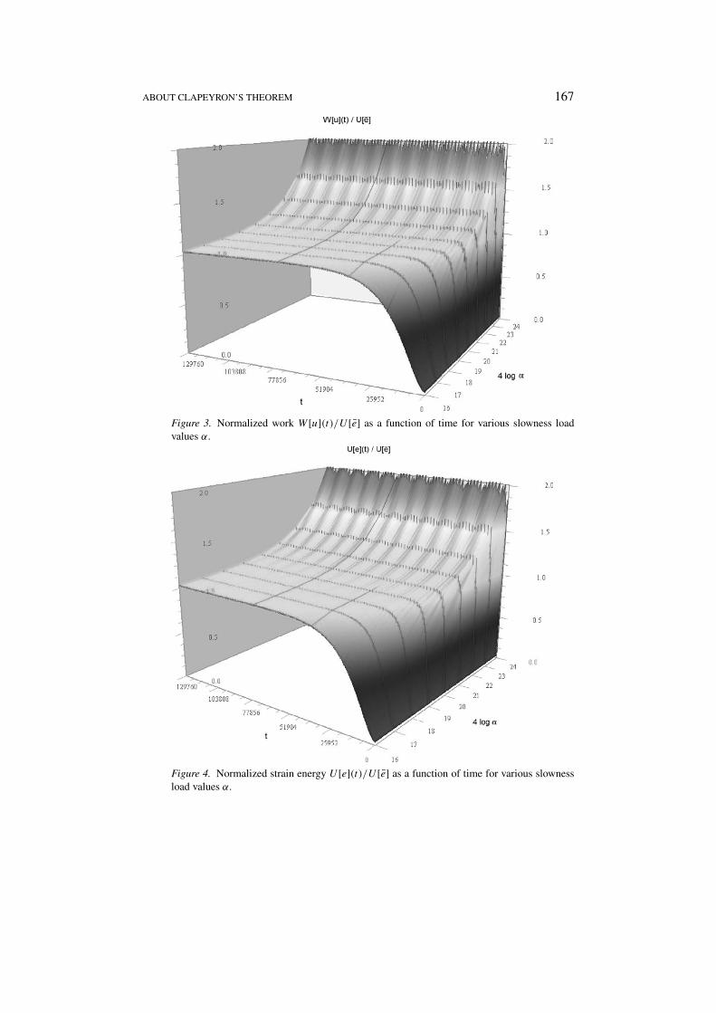
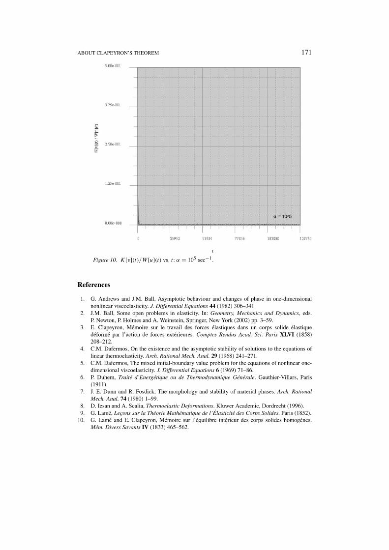
One of the major questions concerning the solution of the dynamical problemstated above is how the work, strain energy and kinetic energy vary with time rela-tive to the strain energy that would be stored in the same elastic bar in equilibriumunder the constant end load σ , i.e., U [e] of (A.7)2. In Figures 3–5 we show thenormalized work,W [u](t)/U [e], normalized strain energy, U [e](t)/U [e], and nor-malized kinetic energy, K[v](t)/U [e], as functions of time computed numericallyfor this problem for a range of slowness load parameters α between α = 104 sec−1

and α = 106 sec−1. These figures are based on material constants for an alu-minum alloy with E = 76.1 × 109 Pa and ρ = 2710 kg/m3, for a bar of lengthL = 5×10−3 m, and for a load constant σ = 107 Pa. The time axis of these figuresis measured in ‘time steps’ with the final time step of 129760 corresponding to1200 × 10−6 sec.

One can see that the impulsive-like nature of the loading for large α resultsin wildly irregular behavior which is sustained over an infinite time. On the con-trary, for relatively small α equilibrium appears to be achieved quickly in timewith nearly constant limiting values W [u](t)/U [e] ≈ 1, U [e](t)/U [e] ≈ 1 andK[v](t)/U [e] ≈ 0. We conclude that the quantity W [u] in (A.7)1, while it hasunits of work and shows up in CLAPEYRON’s theorem as exhibited in (A.6), doesnot represent the work done to reach equilibrium; reasoning based on the computedlimiting behavior leads to the conclusion that only half of this value is expended toreach equilibrium and, then, it is manifested totally in the form of strain energy.


Figure 3. Normalized work W [u](t)/U [e] as a function of time for various slowness loadvalues α.

Figure 4. Normalized strain energy U [e](t)/U [e] as a function of time for various slownessload values α.


Figure 5. Normalized kinetic energy K[v](t)/U [e] as a function of time for various slownessload values α.

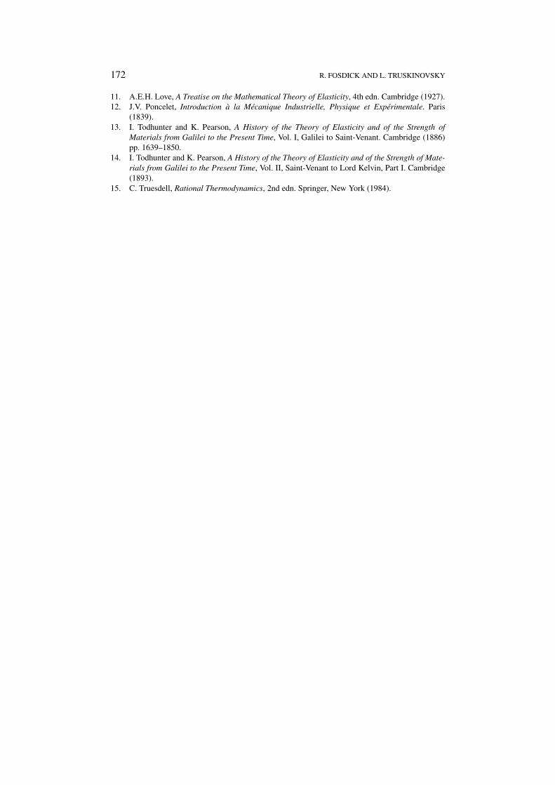
Because there are three decades of variation of the slowness load parameter αshown in Figures 3–5, there is much highly oscillatory, rapid time-behavior that isnot resolved in these figures. Therefore, in Figures 6–10, we take α = 105 sec−1

and show a more detailed solution of (B.1)–(B.3). The material constants E and ρ,bar length L and load constant σ are the same as noted above, but the time stepsfor the time-axis is now such that the final time step of 12800 corresponds to 120×10−6 sec. In Figure 6, we see that the strain field e(x, t) is highly irregular intime at the fixed end x = 0 where information from the time-dependent loadingat the end x = L is reflected back into the bar. The length-axis of this figure ismeasured in ‘length steps’ with the final length step of 100 corresponding to 5 ×10−3 m which is the length of the bar. In Figures 7 and 8, we show the normalizedtotal work done W [u](t)/U [e] and the normalized kinetic energy K[v](t)/U [e]as functions of time. These correspond to the α = 105 sec−1 cross sections ofFigures 3 and 5, respectively, for the initial time interval (0, 12800) as noted inthese figures. The normalized strain energy U [e](t)/U [e] is not shown, but behavessimilar to Figure 7. Notice the orders of magnitude reduction of the energy scaleused in exhibiting the kinetic energy in Figure 8. In Figures 9 and 10, we showthe ratios U [e](t)/W [u](t) and K[v](t)/W [u](t) as functions of time in order toillustrate that it takes only a few ‘rings’ to almost completely eliminate the totalkinetic energy in the bar. Of course, a small motion remains in the bar for all timeno matter how small the slowness parameter α > 0.


Figure 6. Strain e(x, t) as a function of axial position and time for α = 105 sec−1.

Figure 7. W [u](t)/U [e] vs. t : α = 105 sec−1.


Figure 8. K[v](t)/U [e] vs. t : α = 105 sec−1.

Figure 9. U [e](t)/W [u](t) vs. t : α = 105 sec−1.


Figure 10. K[v](t)/W [u](t) vs. t : α = 105 sec−1.

References

1. G. Andrews and J.M. Ball, Asymptotic behaviour and changes of phase in one-dimensionalnonlinear viscoelasticity. J. Differential Equations 44 (1982) 306–341.

2. J.M. Ball, Some open problems in elasticity. In: Geometry, Mechanics and Dynamics, eds.P. Newton, P. Holmes and A. Weinstein, Springer, New York (2002) pp. 3–59.

3. E. Clapeyron, Mémoire sur le travail des forces élastiques dans un corps solide élastiquedéformé par l’action de forces extérieures. Comptes Rendus Acad. Sci. Paris XLVI (1858)208–212.

4. C.M. Dafermos, On the existence and the asymptotic stability of solutions to the equations oflinear thermoelasticity. Arch. Rational Mech. Anal. 29 (1968) 241–271.

5. C.M. Dafermos, The mixed initial-boundary value problem for the equations of nonlinear one-dimensional viscoelasticity. J. Differential Equations 6 (1969) 71–86.

6. P. Duhem, Traité d’Energétique ou de Thermodynamique Générale. Gauthier-Villars, Paris(1911).

7. J. E. Dunn and R. Fosdick, The morphology and stability of material phases. Arch. RationalMech. Anal. 74 (1980) 1–99.

8. D. Iesan and A. Scalia, Thermoelastic Deformations. Kluwer Academic, Dordrecht (1996).9. G. Lamé, Leçons sur la Théorie Mathématique de l’Élasticité des Corps Solides. Paris (1852).

10. G. Lamé and E. Clapeyron, Mémoire sur l’équilibre intérieur des corps solides homogénes.Mém. Divers Savants IV (1833) 465–562.


11. A.E.H. Love, A Treatise on the Mathematical Theory of Elasticity, 4th edn. Cambridge (1927).12. J.V. Poncelet, Introduction à la Mécanique Industrielle, Physique et Expérimentale. Paris

(1839).13. I. Todhunter and K. Pearson, A History of the Theory of Elasticity and of the Strength of

Materials from Galilei to the Present Time, Vol. I, Galilei to Saint-Venant. Cambridge (1886)pp. 1639–1850.

14. I. Todhunter and K. Pearson, A History of the Theory of Elasticity and of the Strength of Mate-rials from Galilei to the Present Time, Vol. II, Saint-Venant to Lord Kelvin, Part I. Cambridge(1893).

15. C. Truesdell, Rational Thermodynamics, 2nd edn. Springer, New York (1984).

About Clapeyron’s Theorem in Linear Elasticity · ABOUT CLAPEYRON’S THEOREM 147 where n is the...

Documents

Transcript of About Clapeyron’s Theorem in Linear Elasticity · ABOUT CLAPEYRON’S THEOREM 147 where n is the...