CENTER for SATELLITE APPLICATIONS and

ALGORITHM THEORETICAL BASIS DOCUMENT

ABI Earth Radiation BudgetUpward Longwave Radiation: TOA

(Outgoing Longwave

Hai-Tien Lee

(2

NOAA NESDIS CENTER for SATELLITE APPLICATIONS and

RESEARCH

ALGORITHM THEORETICAL BASIS DOCUMENT

ABI Earth Radiation BudgetUpward Longwave Radiation: TOA

Outgoing Longwave Radiation

Tien Lee(1), Istvan Laszlo(2) and Arnold Gruber(1)

(1)CICS/ESSIC-NOAA/UMCP

(2)NOAA/NESDIS/STAR, AOSC/UMCP

Version 2.0

1

CENTER for SATELLITE APPLICATIONS and

ALGORITHM THEORETICAL BASIS DOCUMENT

ABI Earth Radiation Budget Upward Longwave Radiation: TOA

Radiation) 1)

2

September 24, 2010

3

TABLE OF CONTENTS 1 INTRODUCTION ........................................................................................................ 9

1.1 Purpose of This Document..................................................................................... 9 1.2 Who Should Use This Document .......................................................................... 9

1.3 Inside Each Section ................................................................................................ 9 1.4 Related Documents ................................................................................................ 9 1.5 Revision History .................................................................................................... 9

2 OBSERVING SYSTEM OVERVIEW....................................................................... 10

2.1 Product Generated ................................................................................................ 10 2.2 Instrument Characteristics ................................................................................... 10

3 ALGORITHM DESCRIPTION.................................................................................. 12

3.1 Algorithm Overview ............................................................................................ 12 3.2 Processing Outline ............................................................................................... 13 3.3 Algorithm Input ................................................................................................... 14

3.3.1 Primary Sensor Data ..................................................................................... 14 3.3.2 Ancillary Data ............................................................................................... 14 3.3.3 Derived Data ................................................................................................. 14

3.4 Theoretical Description ........................................................................................ 14 3.4.1 Physics of the Problem.................................................................................. 14

3.4.1.1 Integral of Electromagnetic Spectrum ................................................... 14

3.4.1.2 Integral of Hemispheric Solid Angles.................................................... 15

3.4.1.3 Integral of Space (Horizontal) ............................................................... 15

3.4.1.4 Integral of Time ..................................................................................... 15

3.4.2 Mathematical Description ............................................................................. 16

3.4.3 Algorithm Output .......................................................................................... 16 3.4.3.1 Output .................................................................................................... 16 3.4.3.2 Quality Flags .......................................................................................... 17

3.4.3.3 Diagnostic Output .................................................................................. 18

4 TEST DATA SETS AND OUTPUTS ........................................................................ 19

4.1 Simulated/Proxy Input Data Sets ......................................................................... 19 4.1.1 SEVIRI Data ................................................................................................. 19

4.2 Output from Simulated/Proxy Inputs Data Sets................................................... 19

4.2.1 Accuracy and Precisions of Estimates .......................................................... 24

4.2.2 Error Budget.................................................................................................. 24 5 PRACTICAL CONSIDERATIONS ........................................................................... 25

5.1 Numerical Computation Considerations .............................................................. 25

5.2 Programming and Procedural Considerations ..................................................... 25

5.3 Quality Assessment and Diagnostics ................................................................... 26

5.4 Exception Handling ............................................................................................. 26 5.5 Algorithm Validation ........................................................................................... 26

6 ASSUMPTIONS AND LIMITATIONS .................................................................... 27

6.1 Performance ......................................................................................................... 27 6.1.1 Graceful Degradation .................................................................................... 27

6.2 Assumed Sensor Performance ............................................................................. 27

6.3 Pre-Planned Product Improvements .................................................................... 27

4

6.3.1 Improvement 1 .............................................................................................. 28 6.3.2 Improvement 2 .............................................................................................. 28

7 REFERENCES ........................................................................................................... 28

5

LIST OF FIGURES Figure 3-1. High level flowchart of the OLR illustrating the main processing sections. . 13

Figure 4-1. OLR validation results for SEVIRI OLR models A and B. .......................... 20

Figure 4-2. Mean and standard deviation of the Model B SEVIRI OLR minus CERES OLR for 1° equal-angle areas. .......................................................................................... 21 Figure 4-3. Spectral minus effective radiances as a function of brightness temperature for the SEVIRI infrared channels (black). The red curves are the differences in the radiance corrections using EUMETSAT versus CICS derived coefficients. These differences are the largest for channel 8 (9.7 µm); an investigation of this large difference is ongoing. . 21 Figure 4-4. Differences in OLR when derived with SEVIRI spectral radiances minus that with the effective radiances as a function of local zenith angle. Number density contour interval is at the power of ten. The SEVIRI radiance errors resulted in limb dependent OLR errors. ....................................................................................................................... 22

Figure 4-5. Mean SEVIRI radiances of channel 5 (6.2 µm) (left) and 9 (10.8 µm) (right) for the validation samples. ................................................................................................ 22 Figure 4-6. SEVIRI OLR errors as function of channel 5 (6.2 µm) radiances for Model B (left) and Model C (right). ................................................................................................ 23 Figure 4-7. Similar to Fig. 2 but is for SEVIRI OLR Model C. ....................................... 23

Figure 4-8. OLR validation results for SEVIRI OLR model C. ....................................... 24

6

LIST OF TABLES

Table 2-1. Channel numbers and wavelengths for the ABI OLR, with information for the corresponding channels for SEVIRI, the developmental surrogate instrument ................ 10

Table 2-2. F&PS requirements for the ABI OLR product. ............................................... 11

Table 4-1. Accuracy and precisions requirement and assessments from current validation studies. .............................................................................................................................. 25

7

LIST OF ACRONYMS

ABI Advanced Baseline Imager AIT Algorithm Integration Team ATBD Algorithm Theoretical Basis Document AWG Algorithm Working Group CERES The Cloud and the Earth’s Radiant Energy System ECT Equator crossing time ERB Earth Radiation Budget F&PS GOES-R Ground Segment Functional and Performance Specification FOV Field of View HIRS High-resolution Infrared Sounder LZA Local zenith angle MRD Mission Requirements Document OLR Outgoing Longwave Radiation SEVIRI Spinning Enhanced Visible and Infrared Imager SSF Single Satellite Footprint TOA Top of the atmosphere

8

ABSTRACT

This is the Algorithm Theoretical Basis Document (ATBD) for the GOES–R Advanced Baseline Imager (ABI) Option-2 Product Upward Longwave Radiation at the top of the atmosphere, also referred to as the outgoing longwave radiation (OLR). This parameter is the total upward thermal radiative flux density emitted by the earth-atmosphere system measured at the top of the atmosphere (TOA) in the unit of watts per square meter. It is one of three radiation budget parameters that determine the earth radiation budget at the TOA. The other two parameters are the incoming solar radiation and the reflected solar radiation. The TOA reflected solar radiation is a GOES-R Baseline product. The Earth Radiation Budget Team of the GOES-R Algorithm Working Group (AWG) prepared this document.

9

INTRODUCTION

1.1 Purpose of This Document The Earth Radiation Budget (ERB) Outgoing Longwave Radiation (OLR) algorithm theoretical basis document (ATBD) provides a high level description of and the physical basis for the technique to estimate the longwave radiative flux at the top of the atmosphere from the measurements of the Advanced Baseline Imager (ABI) flown on the GOES-R series of NOAA’s geostationary meteorological satellites. The OLR is estimated by the radiance observation from each ABI pixel. The OLR is referred to as the upward longwave radiation at top of the atmosphere (TOA) in the Mission Requirements Document (MRD) and the GOES-R Ground Segment Functional and Performance Specification (F&PS).

1.2 Who Should Use This Document The intended users of this document are those interested in understanding the physical basis of the algorithms and the error characteristics of this product. This document also provides information useful to anyone maintaining or modifying the original algorithm.

1.3 Inside Each Section This document is broken down into the following main sections.

• System Overview: Provides relevant details of the ABI and provides a brief description of the product generated by the algorithm.

• Algorithm Description: Provides all the detailed description of the algorithm

including its physical basis, its input and output. • Assumptions and Limitations: Provides an overview of the current limitations of

the approach and gives the plan for overcoming these limitations with further algorithm development.

• Validation: Provides summaries of up to date validation results and descriptions of error characteristics.

1.4 Related Documents Related documents include the specifications of the GOES-R Mission Requirements Document (MRD v3.0), GOES-R Ground Segment Functional and Performance Specification Document (F&PS) and the references given through out.

1.5 Revision History Version 0.1 (Aug. 15, 2008) The Version 0.1 ATBD draft accompanies the delivery of the Version 1 algorithm code package to the GOES-R AWG Algorithm Integration Team (AIT).

10

Version 1.0 (Sep. 26, 2009) Version 1.0 describes the algorithm at the 80% F&PS requirement level, and accompanies the delivery of the Version 4 algorithm code package to the GOES-R AWG Algorithm Integration Team (AIT). Version 2.0 (Sep. 5, 2010) Version 2.0 describes the algorithm at the 100% F&PS requirement level, and accompanies the delivery of the Version 5 algorithm code package to the GOES-R AWG Algorithm Integration Team (AIT). This revision also includes the definitions of metadata, quality flags, and diagnostic output.

2 OBSERVING SYSTEM OVERVIEW This section will describe the product generated by the ABI Outgoing Longwave Radiation (OLR) algorithm and the requirements it places on the sensor.

2.1 Product Generated Retrieval by the OLR algorithm is performed for all ABI pixels. By specification of the MRD, it is responsible for providing one of the TOA Earth Radiation Budget components. The OLR is estimated directly from the ABI radiance, regardless of sky condition. The OLR retrieval can be performed for slant observations up to local zenith angles of 65°. The balance of the following three radiation quantities determines the earth radiation budget at the top of the atmosphere: the incoming total solar radiation (or total solar irradiance; also referred to as the “solar constant” in early literature), the reflected solar radiation, and the outgoing longwave radiation. The TOA reflected solar radiation is a GOES-R baseline product. The GOES-R does not have measurement of the incoming solar radiation, however, as it is a relatively slow varying quantity, it can be estimated from the current solar insolation monitoring missions, including the Active Cavity Radiometer Irradiance Monitor (ACRIM) III on the NASA ACRIMSAT satellite, and the Solar Radiation and Climate Experiment (SORCE)/Total Irradiance Monitor (TIM).

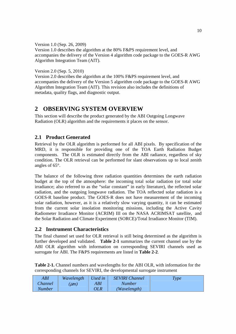
2.2 Instrument Characteristics The final channel set used for OLR retrieval is still being determined as the algorithm is further developed and validated. Table 2-1 summarizes the current channel use by the ABI OLR algorithm with information on corresponding SEVIRI channels used as surrogate for ABI. The F&PS requirements are listed in Table 2-2.

Table 2-1. Channel numbers and wavelengths for the ABI OLR, with information for the corresponding channels for SEVIRI, the developmental surrogate instrument

ABI Channel Number

Wavelength (µm)

Used in ABI OLR

SEVIRI Channel Number

(Wavelength)

Type

11

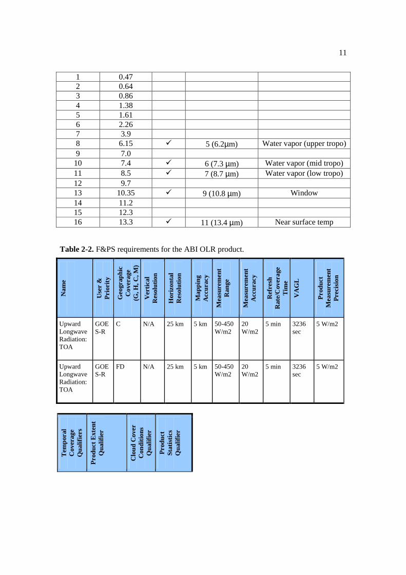
1 0.47 2 0.64 3 0.86 4 1.38 5 1.61 6 2.26 7 3.9 8 6.15 � 5 (6.2µm) Water vapor (upper tropo) 9 7.0 10 7.4 � 6 (7.3 µm) Water vapor (mid tropo) 11 8.5 � 7 (8.7 µm) Water vapor (low tropo) 12 9.7 13 10.35 � 9 (10.8 µm) Window 14 11.2 15 12.3 16 13.3 � 11 (13.4 µm) Near surface temp

Table 2-2. F&PS requirements for the ABI OLR product.

Nam

e

Use

r &

P

rior

ity

Geo

grap

hic

Cov

erag

e (G

, H, C

, M)

Ver

tica

l R

esol

utio

n

Hor

izon

tal

Res

olut

ion

Map

ping

A

ccur

acy

Mea

sure

men

t R

ange

Mea

sure

men

t A

ccur

acy

Ref

resh

R

ate/

Cov

erag

e T

ime

VA

GL

Pro

duct

M

easu

rem

ent

Pre

cisi

on

Upward Longwave Radiation: TOA

GOES-R

C N/A 25 km 5 km 50-450 W/m2

20 W/m2

5 min 3236 sec

5 W/m2

Upward Longwave Radiation: TOA

GOES-R

FD N/A 25 km 5 km 50-450 W/m2

20 W/m2

5 min 3236 sec

5 W/m2

Tem

pora

l C

over

age

Qua

lifie

rs

Pro

duct

Ext

ent

Qua

lifie

r

Clo

ud C

over

C

ondi

tion

s Q

ualif

ier

Pro

duct

St

atis

tics

Q

ualif

ier

12

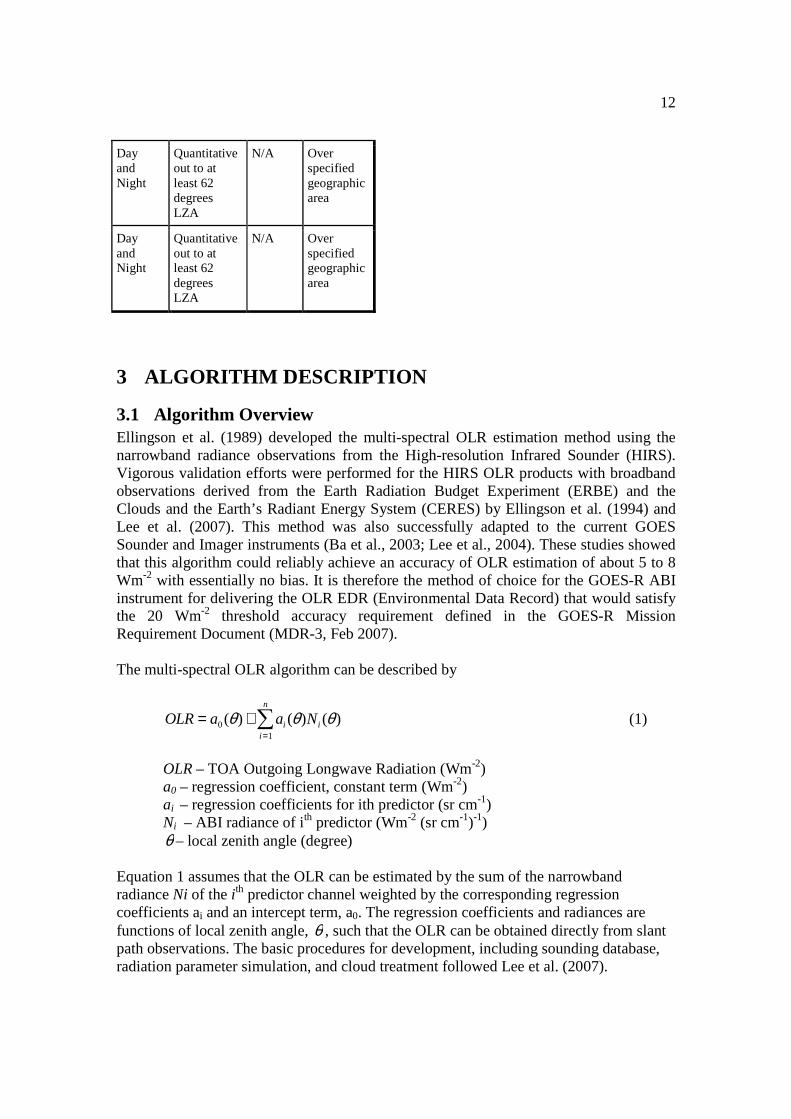
Day and Night

Quantitative out to at least 62 degrees LZA

N/A Over specified geographic area

Day and Night

Quantitative out to at least 62 degrees LZA

N/A Over specified geographic area

3 ALGORITHM DESCRIPTION

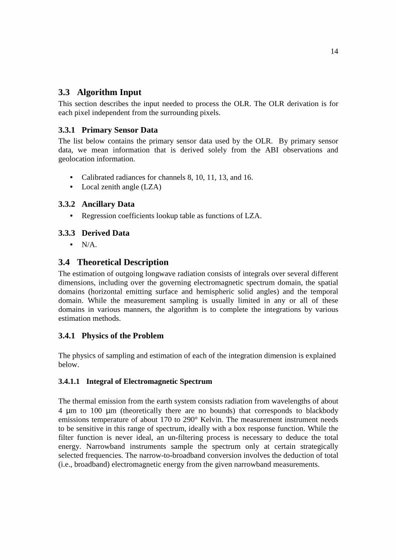
3.1 Algorithm Overview Ellingson et al. (1989) developed the multi-spectral OLR estimation method using the narrowband radiance observations from the High-resolution Infrared Sounder (HIRS). Vigorous validation efforts were performed for the HIRS OLR products with broadband observations derived from the Earth Radiation Budget Experiment (ERBE) and the Clouds and the Earth’s Radiant Energy System (CERES) by Ellingson et al. (1994) and Lee et al. (2007). This method was also successfully adapted to the current GOES Sounder and Imager instruments (Ba et al., 2003; Lee et al., 2004). These studies showed that this algorithm could reliably achieve an accuracy of OLR estimation of about 5 to 8 Wm-2 with essentially no bias. It is therefore the method of choice for the GOES-R ABI instrument for delivering the OLR EDR (Environmental Data Record) that would satisfy the 20 Wm-2 threshold accuracy requirement defined in the GOES-R Mission Requirement Document (MDR-3, Feb 2007). The multi-spectral OLR algorithm can be described by

OLR= a0(θ) + aii =1

n

∑ (θ)Ni (θ ) (1)

OLR – TOA Outgoing Longwave Radiation (Wm-2) a0 – regression coefficient, constant term (Wm-2) ai – regression coefficients for ith predictor (sr cm-1) Ni – ABI radiance of ith predictor (Wm-2 (sr cm-1)-1) θ – local zenith angle (degree)

Equation 1 assumes that the OLR can be estimated by the sum of the narrowband radiance Ni of the i th predictor channel weighted by the corresponding regression coefficients ai and an intercept term, a0. The regression coefficients and radiances are functions of local zenith angle, θ , such that the OLR can be obtained directly from slant path observations. The basic procedures for development, including sounding database, radiation parameter simulation, and cloud treatment followed Lee et al. (2007).

13

3.2 Processing Outline The OLR retrieval is designed to perform on the pixel basis. At each ABI pixel, the ABI radiances are calibrated and navigated to provide longitude, latitude and local zenith angle information. The sensor data input for the OLR algorithm include the radiances of several ABI channels and their local zenith angle. The ancillary data input includes a static regression coefficients lookup table, which is a function of local zenith angle of the observation. There is no input of derived data for OLR retrieval. The output is the OLR assigned to the coordinates of the pixel. For practical programming purpose, the GOES-R rectified grid system might replace the pixel to become the processing unit. The processing outline of the OLR is summarized in Fig. 3-1.

Figure 3-1. High level flowchart of the OLR illustrating the main processing sections.

14

3.3 Algorithm Input This section describes the input needed to process the OLR. The OLR derivation is for each pixel independent from the surrounding pixels.

3.3.1 Primary Sensor Data The list below contains the primary sensor data used by the OLR. By primary sensor data, we mean information that is derived solely from the ABI observations and geolocation information.

• Calibrated radiances for channels 8, 10, 11, 13, and 16. • Local zenith angle (LZA)

3.3.2 Ancillary Data • Regression coefficients lookup table as functions of LZA.

3.3.3 Derived Data • N/A.

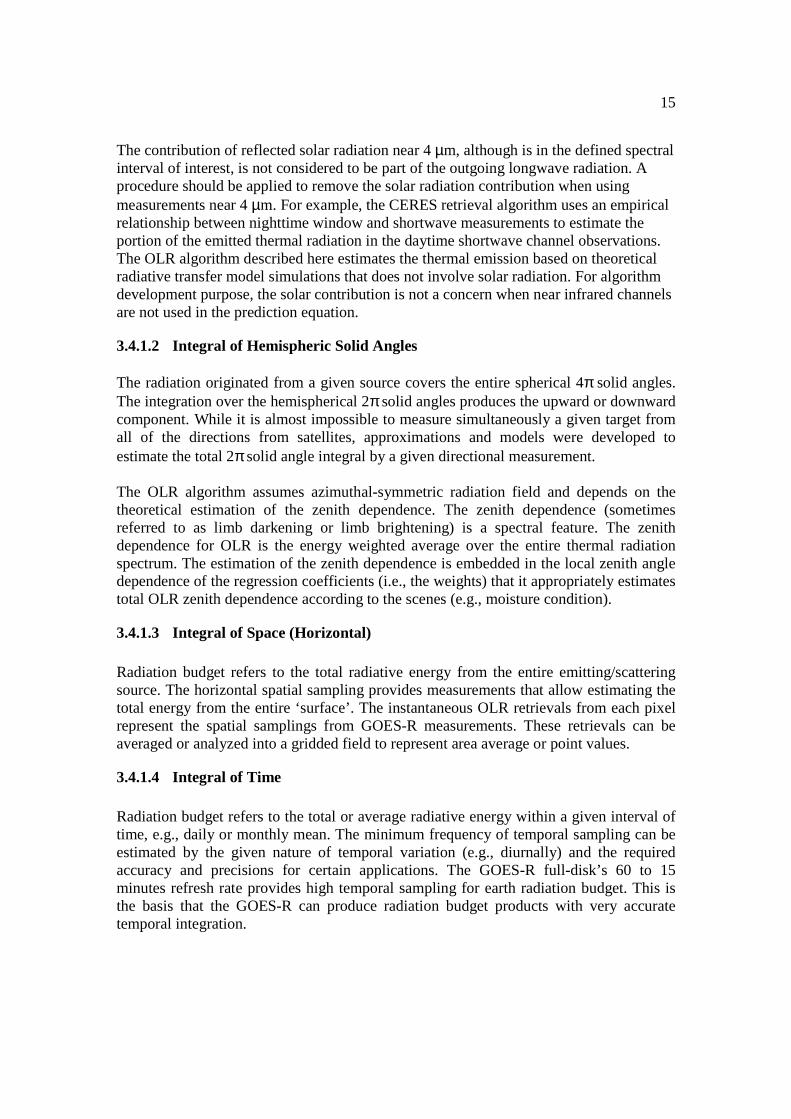
3.4 Theoretical Description The estimation of outgoing longwave radiation consists of integrals over several different dimensions, including over the governing electromagnetic spectrum domain, the spatial domains (horizontal emitting surface and hemispheric solid angles) and the temporal domain. While the measurement sampling is usually limited in any or all of these domains in various manners, the algorithm is to complete the integrations by various estimation methods.

3.4.1 Physics of the Problem The physics of sampling and estimation of each of the integration dimension is explained below.

3.4.1.1 Integral of Electromagnetic Spectrum The thermal emission from the earth system consists radiation from wavelengths of about 4 µm to 100 µm (theoretically there are no bounds) that corresponds to blackbody emissions temperature of about 170 to 290° Kelvin. The measurement instrument needs to be sensitive in this range of spectrum, ideally with a box response function. While the filter function is never ideal, an un-filtering process is necessary to deduce the total energy. Narrowband instruments sample the spectrum only at certain strategically selected frequencies. The narrow-to-broadband conversion involves the deduction of total (i.e., broadband) electromagnetic energy from the given narrowband measurements.

15

The contribution of reflected solar radiation near 4 µm, although is in the defined spectral interval of interest, is not considered to be part of the outgoing longwave radiation. A procedure should be applied to remove the solar radiation contribution when using measurements near 4 µm. For example, the CERES retrieval algorithm uses an empirical relationship between nighttime window and shortwave measurements to estimate the portion of the emitted thermal radiation in the daytime shortwave channel observations. The OLR algorithm described here estimates the thermal emission based on theoretical radiative transfer model simulations that does not involve solar radiation. For algorithm development purpose, the solar contribution is not a concern when near infrared channels are not used in the prediction equation.

3.4.1.2 Integral of Hemispheric Solid Angles The radiation originated from a given source covers the entire spherical 4π solid angles. The integration over the hemispherical 2π solid angles produces the upward or downward component. While it is almost impossible to measure simultaneously a given target from all of the directions from satellites, approximations and models were developed to estimate the total 2π solid angle integral by a given directional measurement. The OLR algorithm assumes azimuthal-symmetric radiation field and depends on the theoretical estimation of the zenith dependence. The zenith dependence (sometimes referred to as limb darkening or limb brightening) is a spectral feature. The zenith dependence for OLR is the energy weighted average over the entire thermal radiation spectrum. The estimation of the zenith dependence is embedded in the local zenith angle dependence of the regression coefficients (i.e., the weights) that it appropriately estimates total OLR zenith dependence according to the scenes (e.g., moisture condition).

3.4.1.3 Integral of Space (Horizontal) Radiation budget refers to the total radiative energy from the entire emitting/scattering source. The horizontal spatial sampling provides measurements that allow estimating the total energy from the entire ‘surface’. The instantaneous OLR retrievals from each pixel represent the spatial samplings from GOES-R measurements. These retrievals can be averaged or analyzed into a gridded field to represent area average or point values.

3.4.1.4 Integral of Time Radiation budget refers to the total or average radiative energy within a given interval of time, e.g., daily or monthly mean. The minimum frequency of temporal sampling can be estimated by the given nature of temporal variation (e.g., diurnally) and the required accuracy and precisions for certain applications. The GOES-R full-disk’s 60 to 15 minutes refresh rate provides high temporal sampling for earth radiation budget. This is the basis that the GOES-R can produce radiation budget products with very accurate temporal integration.

16

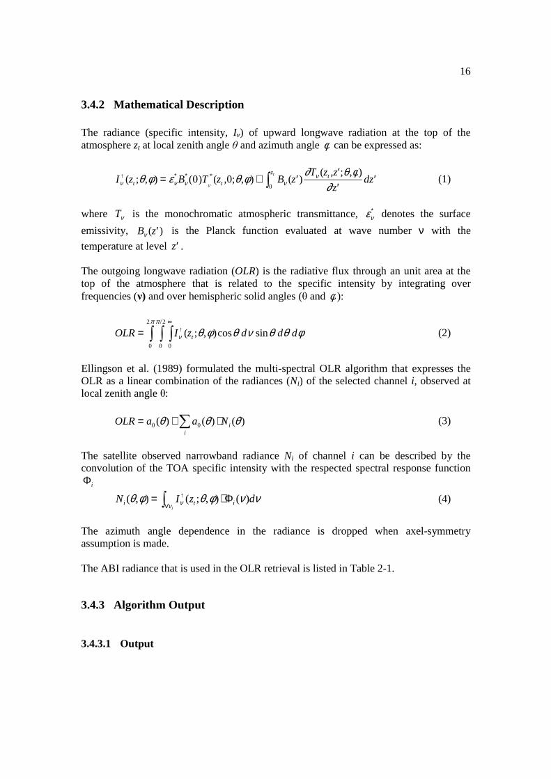
3.4.2 Mathematical Description The radiance (specific intensity, Iν) of upward longwave radiation at the top of the atmosphere zt at local zenith angle θ and azimuth angle φ can be expressed as:

Iν↑(zt ;θ,φ) = εν

∗Bν∗(0)T

ν

* (zt ,0;θ,φ) + Bν ( ′z )∂Tν (zt , ′z ;θ,φ)

∂ ′zd ′z

0

zt

∫ (1)

where Tν is the monochromatic atmospheric transmittance, εν

∗ denotes the surface

emissivity, Bν ( ′z ) is the Planck function evaluated at wave number ν with the

temperature at level ′z . The outgoing longwave radiation (OLR) is the radiative flux through an unit area at the top of the atmosphere that is related to the specific intensity by integrating over frequencies (ν) and over hemispheric solid angles (θ and φ ):

OLR= Iν↑(zt ;θ,φ)cosθ dν sinθ dθ dφ

0

∞

∫0

π /2

∫0

2π

∫ (2)

Ellingson et al. (1989) formulated the multi-spectral OLR algorithm that expresses the OLR as a linear combination of the radiances (Ni) of the selected channel i, observed at local zenith angle θ:

OLR= a0(θ ) + a0(θ ) ⋅ Ni (θ )i∑ (3)

The satellite observed narrowband radiance Ni of channel i can be described by the convolution of the TOA specific intensity with the respected spectral response function Φi

Ni (θ,φ) = Iν↑

Vνi∫ (zt ;θ,φ) ⋅ Φi (ν)dν (4)

The azimuth angle dependence in the radiance is dropped when axel-symmetry assumption is made. The ABI radiance that is used in the OLR retrieval is listed in Table 2-1.

3.4.3 Algorithm Output

3.4.3.1 Output

17

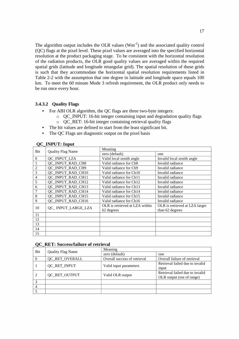
The algorithm output includes the OLR values (Wm-2) and the associated quality control (QC) flags at the pixel level. These pixel values are averaged into the specified horizontal resolution at the product packaging stage. To be consistent with the horizontal resolution of the radiation products, the OLR good quality values are averaged within the required spatial grids (latitude and longitude retangular grid). The spatial resolution of these grids is such that they accommodate the horizontal spatial resolution requirements listed in Table 2-2 with the assumption that one degree in latitude and longitude space equals 100 km. To meet the 60 minute Mode 3 refresh requirement, the OLR product only needs to be run once every hour.

3.4.3.2 Quality Flags

• For ABI OLR algorithm, the QC flags are three two-byte integers: o QC_INPUT: 16-bit integer containing input and degradation quality flags o QC_RET: 16-bit integer containing retrieval quality flags

• The bit values are defined to start from the least significant bit. • The QC Flags are diagnostic output on the pixel basis

QC_INPUT: Input

Bit Quality Flag Name Meaning zero (default) one

0 QC_INPUT_LZA Valid local zenith angle Invalid local zenith angle 1 QC_INPUT_RAD_CH8 Valid radiance for Ch8 Invalid radiance 2 QC_INPUT_RAD_CH9 Valid radiance for Ch9 Invalid radiance 3 QC_INPUT_RAD_CH10 Valid radiance for Ch10 Invalid radiance 4 QC_INPUT_RAD_CH11 Valid radiance for Ch11 Invalid radiance 5 QC_INPUT_RAD_CH12 Valid radiance for Ch12 Invalid radiance 6 QC_INPUT_RAD_CH13 Valid radiance for Ch13 Invalid radiance 7 QC_INPUT_RAD_CH14 Valid radiance for Ch14 Invalid radiance 8 QC_INPUT_RAD_CH15 Valid radiance for Ch15 Invalid radiance 9 QC_INPUT_RAD_CH16 Valid radiance for Ch16 Invalid radiance

10 QC_ INPUT_LARGE_LZA OLR is retrieved at LZA within 62 degrees

OLR is retrieved at LZA larger than 62 degrees

11 12 13 14 15

QC_RET: Success/failure of retrieval

Bit Quality Flag Name Meaning zero (default) one

0 QC_RET_OVERALL Overall success of retrieval Overall failure of retrieval

1 QC_RET_INPUT Valid input parameters Retrieval failed due to invalid input

2 QC_RET_OUTPUT Valid OLR output Retrieval failed due to invalid OLR output (out of range)

3 4 5

18

6 7

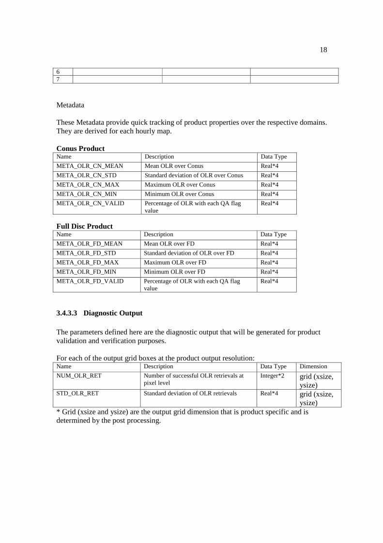
Metadata These Metadata provide quick tracking of product properties over the respective domains. They are derived for each hourly map. Conus Product Name Description Data Type

META_OLR_CN_MEAN Mean OLR over Conus Real*4

META_OLR_CN_STD Standard deviation of OLR over Conus Real*4

META_OLR_CN_MAX Maximum OLR over Conus Real*4

META_OLR_CN_MIN Minimum OLR over Conus Real*4

META_OLR_CN_VALID Percentage of OLR with each QA flag value

Real*4

Full Disc Product Name Description Data Type

META_OLR_FD_MEAN Mean OLR over FD Real*4

META_OLR_FD_STD Standard deviation of OLR over FD Real*4

META_OLR_FD_MAX Maximum OLR over FD Real*4

META_OLR_FD_MIN Minimum OLR over FD Real*4

META_OLR_FD_VALID Percentage of OLR with each QA flag value

Real*4

3.4.3.3 Diagnostic Output The parameters defined here are the diagnostic output that will be generated for product validation and verification purposes. For each of the output grid boxes at the product output resolution: Name Description Data Type Dimension

NUM_OLR_RET Number of successful OLR retrievals at pixel level

Integer*2 grid (xsize, ysize)

STD_OLR_RET Standard deviation of OLR retrievals Real*4 grid (xsize, ysize)

* Grid (xsize and ysize) are the output grid dimension that is product specific and is determined by the post processing.

19

4 TEST DATA SETS AND OUTPUTS

4.1 Simulated/Proxy Input Data Sets The ABI OLR algorithm is evaluated with the SEVERI surrogate algorithm.

4.1.1 SEVIRI Data The SEVIRI radiance data from June 21-27 and December 11-17, 2004 over the Meteosat-8 (Schmetz et al., 2002) full disk domain were collocated with CERES Single Scanner Footprint (SSF) data from all four instruments, FM1 & 2 (Ed.2B) and FM3 & 4 (Ed.1B), onboard the Terra and Aqua satellites, respectively. The SEVIRI radiance observations were averaged for 3x3 pixels (native resolution is 3 km at the sub-satellite point) centered on the CERES footprint (about 20 km nadir). Homogeneity indicators are defined for the 0.6-µm and 10.8-µm channels as the ratio of the difference of the maximum and minimum values to the mean for each of the 3x3-pixel SEVIRI area. Homogeneous scenes are filtered through this indicator at a threshold of 0.01 for the 10.8-µm channel. The homogeneity indicator derived from the visible channel is not used. The temporal matching window is ±7.5 minutes.

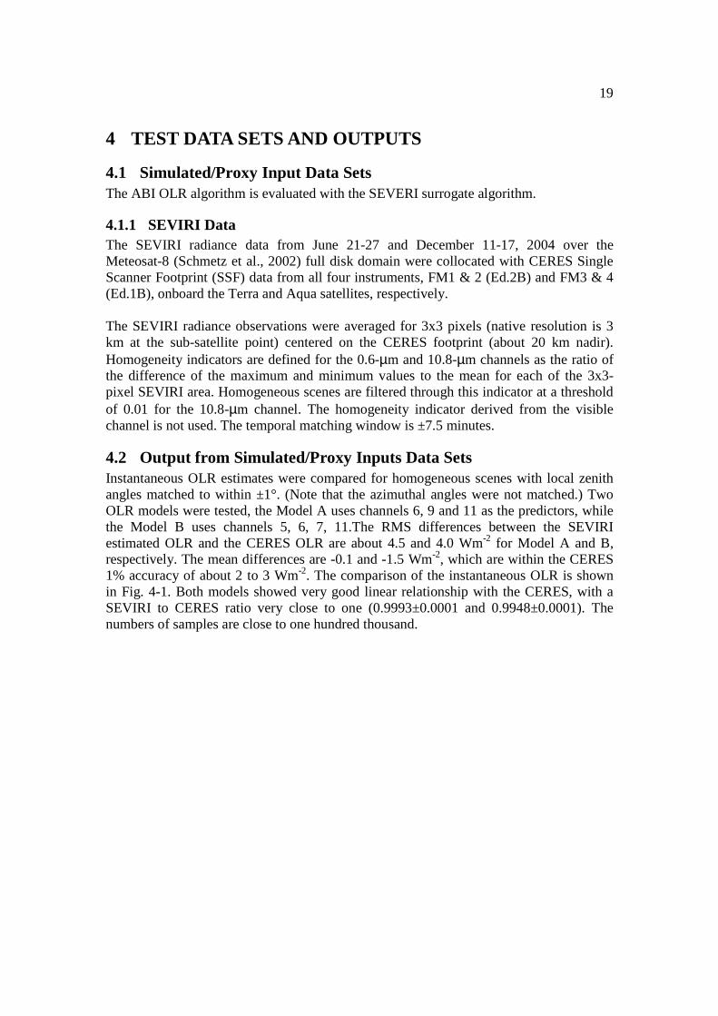
4.2 Output from Simulated/Proxy Inputs Data Sets Instantaneous OLR estimates were compared for homogeneous scenes with local zenith angles matched to within ±1°. (Note that the azimuthal angles were not matched.) Two OLR models were tested, the Model A uses channels 6, 9 and 11 as the predictors, while the Model B uses channels 5, 6, 7, 11.The RMS differences between the SEVIRI estimated OLR and the CERES OLR are about 4.5 and 4.0 Wm-2 for Model A and B, respectively. The mean differences are -0.1 and -1.5 Wm-2, which are within the CERES 1% accuracy of about 2 to 3 Wm-2. The comparison of the instantaneous OLR is shown in Fig. 4-1. Both models showed very good linear relationship with the CERES, with a SEVIRI to CERES ratio very close to one (0.9993±0.0001 and 0.9948±0.0001). The numbers of samples are close to one hundred thousand.

20

Figure 4-1. OLR validation results for SEVIRI OLR models A and B.

21

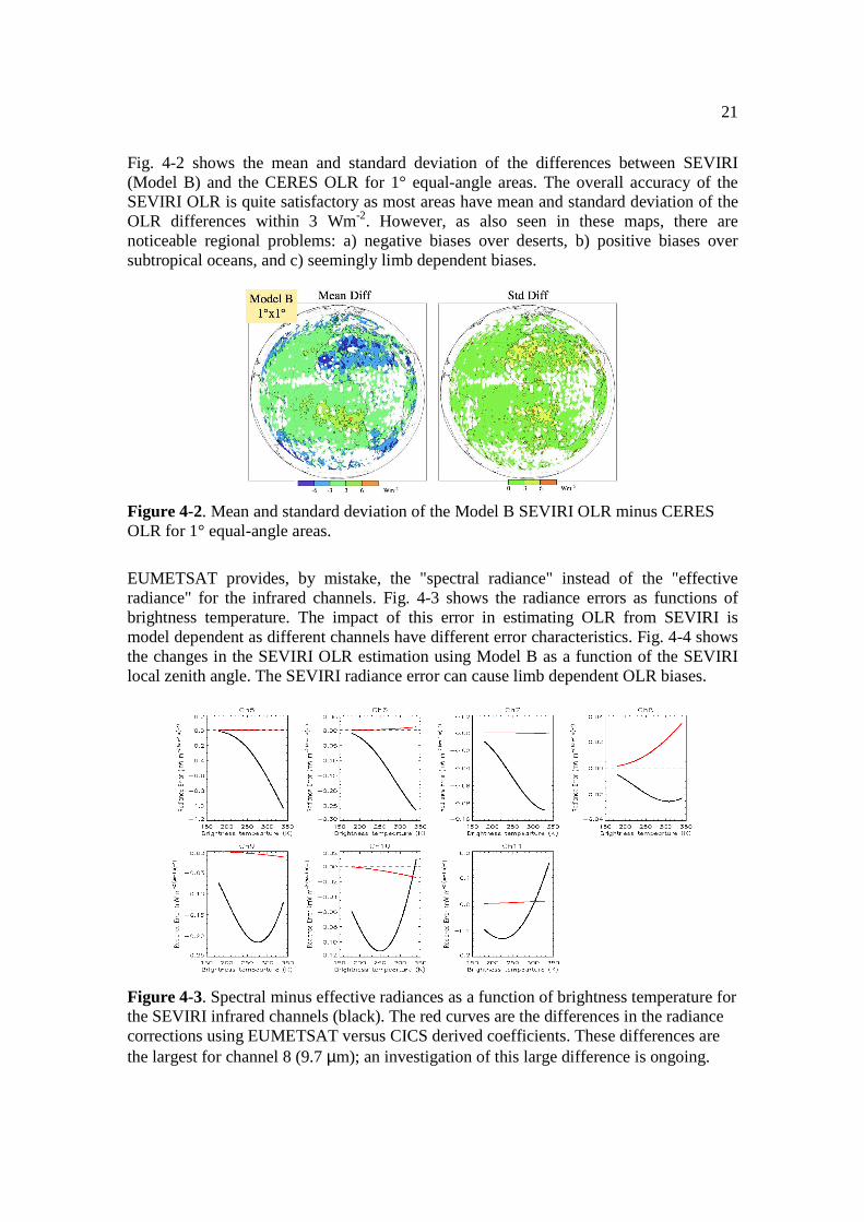
Fig. 4-2 shows the mean and standard deviation of the differences between SEVIRI (Model B) and the CERES OLR for 1° equal-angle areas. The overall accuracy of the SEVIRI OLR is quite satisfactory as most areas have mean and standard deviation of the OLR differences within 3 Wm-2. However, as also seen in these maps, there are noticeable regional problems: a) negative biases over deserts, b) positive biases over subtropical oceans, and c) seemingly limb dependent biases.

Figure 4-2. Mean and standard deviation of the Model B SEVIRI OLR minus CERES OLR for 1° equal-angle areas.

EUMETSAT provides, by mistake, the "spectral radiance" instead of the "effective radiance" for the infrared channels. Fig. 4-3 shows the radiance errors as functions of brightness temperature. The impact of this error in estimating OLR from SEVIRI is model dependent as different channels have different error characteristics. Fig. 4-4 shows the changes in the SEVIRI OLR estimation using Model B as a function of the SEVIRI local zenith angle. The SEVIRI radiance error can cause limb dependent OLR biases.

Figure 4-3. Spectral minus effective radiances as a function of brightness temperature for the SEVIRI infrared channels (black). The red curves are the differences in the radiance corrections using EUMETSAT versus CICS derived coefficients. These differences are the largest for channel 8 (9.7 µm); an investigation of this large difference is ongoing.

22

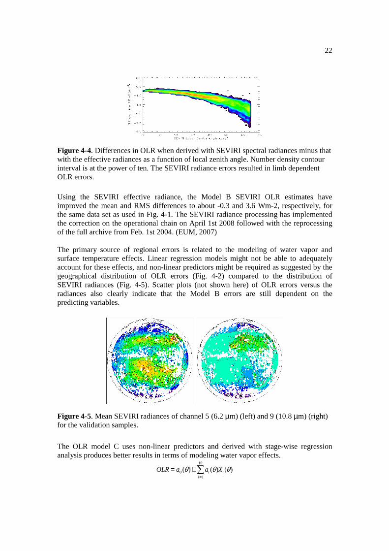
Figure 4-4. Differences in OLR when derived with SEVIRI spectral radiances minus that with the effective radiances as a function of local zenith angle. Number density contour interval is at the power of ten. The SEVIRI radiance errors resulted in limb dependent OLR errors.

Using the SEVIRI effective radiance, the Model B SEVIRI OLR estimates have improved the mean and RMS differences to about -0.3 and 3.6 Wm-2, respectively, for the same data set as used in Fig. 4-1. The SEVIRI radiance processing has implemented the correction on the operational chain on April 1st 2008 followed with the reprocessing of the full archive from Feb. 1st 2004. (EUM, 2007) The primary source of regional errors is related to the modeling of water vapor and surface temperature effects. Linear regression models might not be able to adequately account for these effects, and non-linear predictors might be required as suggested by the geographical distribution of OLR errors (Fig. 4-2) compared to the distribution of SEVIRI radiances (Fig. 4-5). Scatter plots (not shown here) of OLR errors versus the radiances also clearly indicate that the Model B errors are still dependent on the predicting variables.

Figure 4-5. Mean SEVIRI radiances of channel 5 (6.2 µm) (left) and 9 (10.8 µm) (right) for the validation samples.

The OLR model C uses non-linear predictors and derived with stage-wise regression analysis produces better results in terms of modeling water vapor effects.

OLR= a0(θ) + ai (θ)i =1

10

∑ Xi (θ)

23

X = [N5,N6,N7,N11],[ N52,N6

2,N63,N9 ],[ N11

2 ,N113 ]{ }

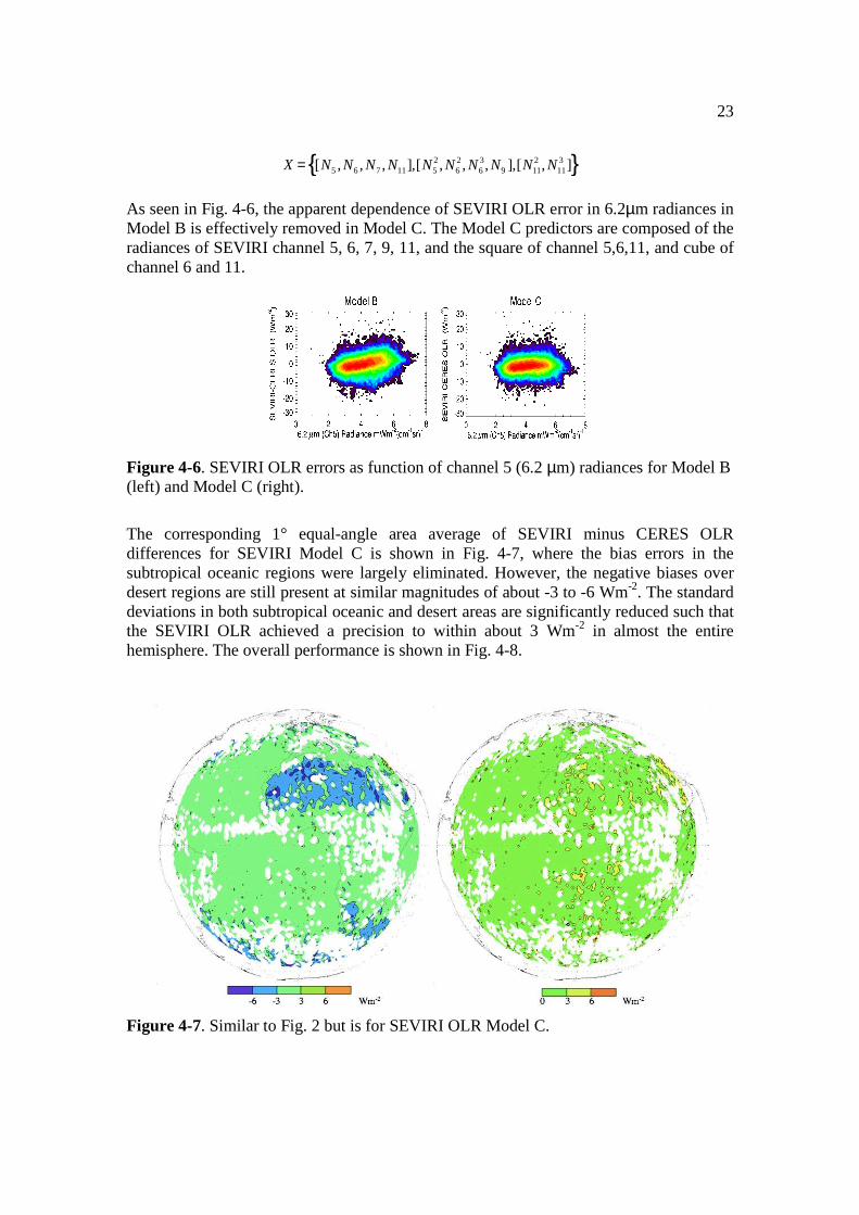
As seen in Fig. 4-6, the apparent dependence of SEVIRI OLR error in 6.2µm radiances in Model B is effectively removed in Model C. The Model C predictors are composed of the radiances of SEVIRI channel 5, 6, 7, 9, 11, and the square of channel 5,6,11, and cube of channel 6 and 11.

Figure 4-6. SEVIRI OLR errors as function of channel 5 (6.2 µm) radiances for Model B (left) and Model C (right).

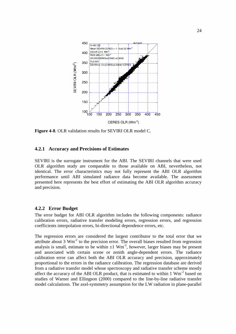
The corresponding 1° equal-angle area average of SEVIRI minus CERES OLR differences for SEVIRI Model C is shown in Fig. 4-7, where the bias errors in the subtropical oceanic regions were largely eliminated. However, the negative biases over desert regions are still present at similar magnitudes of about -3 to -6 Wm-2. The standard deviations in both subtropical oceanic and desert areas are significantly reduced such that the SEVIRI OLR achieved a precision to within about 3 Wm-2 in almost the entire hemisphere. The overall performance is shown in Fig. 4-8.

Figure 4-7. Similar to Fig. 2 but is for SEVIRI OLR Model C.

24

Figure 4-8. OLR validation results for SEVIRI OLR model C.

4.2.1 Accuracy and Precisions of Estimates SEVIRI is the surrogate instrument for the ABI. The SEVIRI channels that were used OLR algorithm study are comparable to those available on ABI, nevertheless, not identical. The error characteristics may not fully represent the ABI OLR algorithm performance until ABI simulated radiance data become available. The assessment presented here represents the best effort of estimating the ABI OLR algorithm accuracy and precision.

4.2.2 Error Budget The error budget for ABI OLR algorithm includes the following components: radiance calibration errors, radiative transfer modeling errors, regression errors, and regression coefficients interpolation errors, bi-directional dependence errors, etc. The regression errors are considered the largest contributor to the total error that we attribute about 3 Wm-2 to the precision error. The overall biases resulted from regression analysis is small, estimate to be within ±1 Wm-2, however, larger biases may be present and associated with certain scene or zenith angle-dependent errors. The radiance calibration error can affect both the ABI OLR accuracy and precision, approximately proportional to the errors in the radiance calibration. The regression database are derived from a radiative transfer model whose spectroscopy and radiative transfer scheme mostly affect the accuracy of the ABI OLR product, that is estimated to within 1 Wm-2 based on studies of Warner and Ellingson (2000) compared to the line-by-line radiative transfer model calculations. The axel-symmetry assumption for the LW radiation in plane-parallel

25

calculation is valid for most situations, however, the shadows from either the persistent cloud and terrain could impose a non-negligible azimuth dependence in the LW radiance, thus leads to biases in the OLR. The magnitude of these errors is yet uncertain. Table 4-1 lists the accuracy and precision estimation for ABI OLR algorithm based on the validation study for the SEVIRI derived OLR. For instantaneous SEVIRI OLR retrievals compared to the CERES OLR from all four flight-models, the SEVIRI OLR retrieval has a bias of -1.15 ±0.02 Wm-2, and a standard deviation of OLR differences of 2.9 Wm-2. Current assessment suggests that the overall accuracy and precision for the ABI OLR algorithm are 2 and 4 Wm-2, respectively. The performance of this OLR algorithm is considered to have met the 100% F&PS requirements.

Table 4-1. Accuracy and precisions requirement and assessments from current validation studies.

F&PS Algorithm Evaluation

Wm-2 Accuracy Precision Range Accuracy Precision

OLR 20 5 50-450 2 4 Offline Studies

5 PRACTICAL CONSIDERATIONS

5.1 Numerical Computation Considerations OLR retrieval is performed on the pixel basis, independent from other pixels. This is ideal for vector processing. Although the flow chart is now designed for pixel processing, it would be more efficient to extend it to one scan unit, or the next larger processing unit, e.g., a granule.

5.2 Programming and Procedural Considerations The OLR algorithm is designed to be a pixel-based algorithm with the inputs of the calibrated ABI radiance, and the navigation and observation geometry information. The only ancillary data is a static regression coefficients table. It should stay with the rest of the Earth radiation budget production modules at near the end of the production chain where most atmospheric and surface retrievals have been performed and are available to the earth radiation budget derivation whenever needed.

26

5.3 Quality Assessment and Diagnostics Depending on the availability and timeliness of the reference data sets, there are several levels of quality assessment (QA) and diagnostics. The following procedures are recommended for diagnosing the performance of the OLR. Real Time

• HIRS OLR • CERES OLR (from NPP and JPSS-1 Flashflux product)

Near Real-time • NWP 6-hr Radiation Flux fields forecast • RTM calc. w/ NWP analysis, w/ TOA tuning

Offline • CERES OLR and CERES SARB (currently with 6 months lag)

For each level, the evaluation methods will be defined, e.g., domain mean differences, standard deviation of differences, time series analysis, etc. To automate the product monitoring, a set of gross check thresholds needs to be defined to alert production problems. These thresholds are determined through the algorithm development/validation and framework validation studies. The real time evaluation and monitoring are routine procedures to be attached to the production system. A set of simple statistics will be generated to give some indication of the quality and consistency of the product. The offline evaluation provides the best assessment of the product accuracy and uncertainty; however, there will be a time lag of about from 3 months to a year.

5.4 Exception Handling The ABI radiance data used in OLR retrieval will be checked for QA flags. The OLR retrieval will proceed only when the radiance from all needed channels have good quality flag. The navigation of satellite produces the local zenith angle for each scanning pixel. The accuracy of that angle is crucial to the OLR retrieval. The quality of local zenith angle derivation by the navigation package is assumed to be correct at all time. The OLR is checked against the specified OLR range, from 50 Wm-2 to 450 Wm-2. The missing value will be assigned when calculation results are outside the allowed range.

5.5 Algorithm Validation The primary reference source for algorithm validation is from the broadband radiative flux product derived from the CERES observations. The availability of this product however usually has a typical lag time of six months. This is not a concern for offline product validation and assessment; however, until the operational broadband radiation budget production from NPOESS/NPP becomes available, we need to consider other data

27

sources for product assessment. For the moment, the real-time product quality assessment and monitoring will be using the HIRS OLR product as it is operationally generated and will be available throughout MetOp-B. On MetOp-C, the IASI OLR product will be generated and replaces the HIRS OLR product for operational quality assurance and monitoring purpose.

6 ASSUMPTIONS AND LIMITATIONS The following sections describe the current limitations and assumptions in the current version of the OLR.

6.1 Performance The ABI OLR algorithm is evaluated using a surrogate SEVERI OLR algorithm. The evaluation of ABI OLR algorithm is possible when quality simulation data is available. The retrieval performance assessed for SEVIRI OLR algorithm should represent that of the ABI OLR algorithm.

6.1.1 Graceful Degradation Local Zenith Angle Limitation The F&PS required range of local zenith angle (LZA) for OLR retrieval is up to 62 degrees. The OLR retrieval quality degrades significantly for the very large angles (>~70°). Currently the OLR regression coefficients database is derived for LZA up to 65 degrees. The OLR retrievals at LZA equal or greater than 62 degrees are generated but are expected to have a slightly lower quality. Availability of Radiances Although it is possible to determine alternative set of radiances to perform OLR retrieval, no alternative set is derived currently. Therefore the OLR retrieval will report missing value if any of the radiance QC flags of the required channels (channels 8, 10, 11, 13, 16) was turned on.

6.2 Assumed Sensor Performance The OLR retrieval accuracy can be affected by the radiance calibration and navigation. The errors in radiance calibration and derivation of local zenith angle can propagate into OLR retrieval in both forms of biases and noises that will affect the accuracy and precision of the retrievals.

6.3 Pre-Planned Product Improvements The overall performance of the ABI OLR algorithm is very satisfactory, however, there are still some regional bias problems (e.g., over the desert). The proposed version 1 algorithm involves using non-linear predictors that are potentially less stable than those with linear predictors. More detailed examinations and validation case studies are necessary to further improve confidence in this algorithm. Studies using ABI simulation data would be very useful in pre-launch testing.

28

6.3.1 Improvement 1 OLR Algorithm (General) During the algorithm validation study, the limb dependent biases were identified and were corrected using higher order predictor terms in the OLR regression model. The first order linear approximation that converts narrowband to broadband can produce biases when the samples are not ‘sufficiently diversified’ (as what regression is designed for). The geostationary observing geometry does collect samples at less diversified fashion, including the local zenith angles, climate types, etc. These are likely sources of bias errors in the OLR retrievals. Scene dependent application may be necessary to completely eliminate these types of errors. Higher order of estimation function in both spectral domain and in the angular model can also improve the regional accuracy when nonlinearity is more accurately described. Regression models developed for subsets of spectral intervals can also reduce the possible biases within extreme and rare types of climate zones. These are the possible future improvements for the OLR algorithm that will likely fix existing problems, e.g., over-estimation in the desert regions and to improve the overall accuracy and precision.

6.3.2 Improvement 2 Sky conditions Introduction of scene dependency on cloud amount and type is a very plausible improvement in OLR estimation accuracy, particularly with the semi-transparent cirrus. The side effect of this implementation is, however, to become dependent on the precedent cloud products. The net gain from this implementation is uncertain at the moment.

7 REFERENCES Ba, M., R. G. Ellingson and A. Gruber, 2003: Validation of a technique for estimating OLR with the GOES sounder. J. Atmos. Ocean. Tech., 20, 79-89. Ellingson, R. G., D. J. Yanuk, H.-T. Lee and A. Gruber, 1989: A technique for estimating outgoing longwave radiation from HIRS radiance observations. J. Atmos. Ocean. Tech., 6, 706-711. Ellingson, R. G., H.-T. Lee, D. Yanuk and A. Gruber, 1994: Validation of a technique for estimating outgoing longwave radiation from HIRS radiance observations, J. Atmos. Ocean. Tech., 11, 357-365. EUM, 2007: A Planned Change to the MSG Level 1.5 Image Product Radiance Definition. EUM/OPS- MSG/TEN/06/0519 v1A. 5 January 2007. Lee, H.-T., A. Gruber, R. G. Ellingson and I. Laszlo, 2007: Development of the HIRS Outgoing Longwave Radiation climate data set. J. Atmos. Ocean. Tech., 24, 2029–2047.

29

Lee, H.-T., A. Heidinger, A. Gruber and R. G. Ellingson, 2004: The HIRS Outgoing Longwave Radiation product from hybrid polar and geosynchronous satellite observations. Advances in Space Research, 33, 1120-1124. Schmetz, J., Pili, P., Tjemkes, S., Just, D., Kerkmann, J., Rota, S., and Ratier, A., (2002) An introduction to Meteosat Second Generation (MSG). Bulletin of the American Meteorological Society, 83, 977-992. Warner, J. X. and R. G. Ellingson, 2000: A new narrowband radiation model for water vapor absorption. J. Atmos. Sci., 57, 1481-1496