Abdulkadir, M. and Hernandez-Perez, V. and Lowndes, Ian and Azzopardi, Barry J. and Dzomeku, S. (2014) Experimental study of the hydrodynamic behaviour of slug flow in a vertical riser. Chemical Engineering Science, 106 . pp. 60-75. ISSN 1873-4405

Access from the University of Nottingham repository: http://eprints.nottingham.ac.uk/35518/1/MANUSCRIPT%20%28SLUG%20FLOW%20IN%20A%20VERTICAL%20RISER%29.pdf

Copyright and reuse:

The Nottingham ePrints service makes this work by researchers of the University of Nottingham available open access under the following conditions.

This article is made available under the Creative Commons Attribution Non-commercial No Derivatives licence and may be reused according to the conditions of the licence. For more details see: http://creativecommons.org/licenses/by-nc-nd/2.5/

A note on versions:

The version presented here may differ from the published version or from the version of record. If you wish to cite this item you are advised to consult the publisher’s version. Please see the repository url above for details on accessing the published version and note that access may require a subscription.

For more information, please contact eprints@nottingham.ac.uk

1 | P a g e

Experimental study of the hydrodynamic behaviour of slug flow in a vertical riser

M. Abdulkadir*1, V. Hernandez-Perez1, I. S. Lowndes1, B. J. Azzopardi1 and S. Dzomeku2

1Process and Environmental Engineering Research Division, Faculty of Engineering, University of Nottingham

University Park, Nottingham, NG7 2RD, United Kingdom

2Petroleum Engineering Department, African University of Science and Technology (AUST), Abuja, Nigeria

*Email of the corresponding author: mukhau@futminna.edu.ng

Abstract: This paper presents an investigation of the hydrodynamics of slug flow in a vertical 67 mm internal

diameter riser. The slug flow regime was generated using a multiphase air-silicone oil mixture over a range of

gas (0.42< USG< 1.35 m/s) and liquid (0.05<USL< 0.38 m/s) superficial velocities. Electrical Capacitance

Tomography (ECT) was used to determine: the velocities of the Taylor bubbles and liquid slugs, the slug

frequencies, the lengths of Taylor bubbles and the liquid slugs, the void fractions within the Taylor bubbles and

liquid slugs and the liquid film thicknesses. A differential pressure transducer was used to measure the pressure

drops along the length of the riser. It was found that the translational velocity of a Taylor bubble (the structure

velocity) was strongly dependent on the mixture superficial velocity. As the gas superficial velocity, was

increased, the void fraction and the lengths of the liquid slugs and the Taylor bubbles were observed to increase.

The increase in gas superficial velocity causes an increase in the frictional pressure drop within the pipe, whilst

the total pressure drop (which is a sum of the hydrostatic and frictional pressure drop) along the length of the

riser decreases. In addition, the frequencies of the liquid slugs were observed to increase as the liquid superficial

velocity increases, but to be weakly dependant on the gas superficial velocity. The manual counting method for

the determination of slug frequency was found to be in good agreement with the power spectral density (PSD)

computed method.

Key words: ECT, Taylor bubble, liquid slug, slug unit, frequency, void fraction

1.0 Introduction:

Slug flow occurs in horizontal, inclined and vertical pipes over a wide range of liquid and gas flow rates. It is

the dominant flow pattern in upward inclined flow. The flow is associated with operational problems such as

operation, erosion-corrosion enhancement, and structural problems occurring most especially in bends. Slug

flow hydrodynamics is complex with unsteady flow behaviour characteristics. It has peculiar velocity and

2 | P a g e

pressure distributions. Therefore, the predictions of the liquid holdup, pressure drop, heat transfer, mass transfer

are difficult and challenging.

The power, nuclear and chemical industries have provided a platform for strong interest in multiphase flow

study. Examples of such studies are steam-water flow for power generation and flow reactors for heat and mass

transfer. Additionally, applications in the petroleum industry provide another strong motivation for multiphase

flow research. The transportation of multiphase involving, oil and gas in pipes is significantly reducing the cost

of reservoir development. However, the main challenge confronting them is the development of multiphase

technology for the transportation of oil and gas from subsea production units at large water depths to processing

facilities at nearby platforms or onshore facilities. The flows in the subsea pipelines usually contain multiple

phases, like oil, water and /or gas, whose composition is not known priori. The variation in the composition of

fluids inside the long subsea network can lead to serious operational problems, ranging from non -continuous

production or shut-down to damage equipment.

Gas with large amounts of water and or oil-water mixtures may be produced simultaneously, resulting in

multiphase flow conditions in the transporting pipe system between the source and the production platform. As

the fields grow older, the produced gas contains an increasing amount of water, giving rise to different mixture

compositions, which affect the flow pattern and flow characteristics (Zoeteweij (2007)). For upward inclined

and vertical pipe flow, s lug flow can be considered as the dominant flow pattern, Hernandez-Perez (2008). This

can enhance corrosion, as Kaul (1996) noted that the corrosion rate is accelerated when the flow pattern is slug

flow. This flow pattern is usually characterised by an alternating flow of gas pockets and liquid slugs. Mos t of

the gas-phase is concentrated in large bullet-shaped gas pockets, defined as Taylor bubbles. The Taylor bubbles

are separated by intermediate liquid slugs, which may contain small entrained gas bubbles. A major

characteristic of slug flows are their inherent unsteadiness. As this kind of flow occurs over a wide range of

intermediate flow rates of gas and liquid, it is of major interest to a wide range of industrial processes that

employ pipeline transport systems.

The presence of liquid slugs in the flow system gives an irregular output in terms of gas and liquid flow at the

outlet of the system, or at the next processing stage. This can pose problems to the designer and operator of two-

phase flow systems. Pressure drop is substantially higher in slug flow as compared to other flow regimes, and

the maximum possible length of a liquid slug that might be encountered in the flow system needs to be known ,

3 | P a g e

Abdulkadir (2011). In the 67 mm facility used in the current study, slugs were observed to be of about 10 pipe

diameters in length, i.e. long enough for the rise velocity to be independent of the length Griffith and Wallis

(1961). For large capacity systems in industry, these liquid slugs can even grow longer, carrying large

momentum. Often, slug catching devices are used to collect the slugs, and avoid any damage to the downstream

equipment. For the design of such slug catchers, it is important to know what kind of slugs to anticipate. The

important question of when, and how, these slugs are formed has received much attention from research workers

Abdulkadir (2011). However, reports on the study of the behaviour of these slugs in more industry relevant

fluids are limited. For that reason, it is important to study the behaviour of slug flow in great detail for the

optimal, efficient and safe design and operation of two-phase gas-liquid slug flow systems.

An analysis of the ECT data enabled the characterisation of the slug flow. This enabled the measurement of the

instantaneous distribution of the flow phases over the cross-section of the pipe. The use of two such

circumferential rings of sensor electrodes , 89 mm apart (also known as twin-plane sensors), enabled the

determination of the translational velocity of the observed Taylor bubbles and liquid slugs. With this

information, a more fundamental approach is used for improving the general knowledge on slug flow.

1.1 Background:

The occurrence of slug flow in a vertical riser is a very common phenomenon under normal operating conditions

within a two-phase flow facility, such as in an oil production riser. Over the past thirty years there have been a

large number of research studies in this field in the peer review literature.

One of the earliest contributions to slug flow characterization was carried out by Nicklin et al. (1962), who

proposed an empirical relationship to describe the rise velocity of single Taylor air bubble in a static water

column. Nicklin’s empirical relationship, given by equation (1), describes the translational velocity of a Taylor

bubble, UN, it is the sum of the Taylor bubble rise velocity, or drift velocity, which is the velocity of a Taylor

bubble in a stagnant liquid, plus the contribution of the mixture superficial velocity in the preceding slug . For

the air-water system in a 26 mm bore tube considered the values of the constants oC and k were determined to

be 1.2 and 0.35, respectively.

gDkUCU MoN (1)

4 | P a g e

Where C0 is a flow distribution coefficient, k is drift coefficient, UM is the mixture superficial velocity and

gDk is the drift velocity.

Moissis (1963) agreed that NU predicted by equation (1) fitted his data well. Akagawa and Sakaguchi (1966)

confirm the applicability of equation (1) to the air-water system in a 26 mm diameter pipe and pointed out the

effect of the term gDk is negligible except at low gas and liquid velocities. They suggested that the presence

of small bubbles in the liquid slug has a slight effect on the translational velocity of a Taylor bubble and that

their data indicated that 0C is in the range of 1.25 - 1.35.

Brown (1965) found experimentally that the analytical solutions for the translational velocity of a Taylor bubble

derived by Dumitrescu (1943) and Davies and Taylor (1950) described the behaviour of gas bubbles in low

viscosity liquids well, however they were not suitable for high viscosity liquids.

Vince and Lahey (1982) claimed that excellent correlation between the translational velocity of a Taylor bubble,

NU and the mixture superficial velocity, MU was given by the equation (2):

15.029.1 MN UU (2)

Following an analysis of experimental data in a 50 mm diameter tube, Fernandes et al. (1983) determined a

slightly higher value of 1.29 for0C . They ascribed the increase in the constant

0C to diameter effect or to the

contribution made by heading and trailing Taylor bubbles. Barnea and Shemer (1989) verified equation (1),

using their own measurements on a 50 mm diameter tube, and used it in their calculations. A more physically

based interpretation of the proposed increase in the constant was later provided by Mao and Dukler (1985).

They used an aqueous electrolytic solution and air in a 50.8 mm diameter tube. They took into consideration the

fact that the liquid slug in front of a Taylor bubble is aerated, and coalescence takes place between the small

bubbles and the Taylor bubbles . This results in an increase of the velocity of the Taylor bubble. They derived a

mathematical relationship to determine the translational velocity of a Taylor bubbles, equation (3).

NLLSoN UgDUCU 35.0 (3)

where,

5 | P a g e

ULLS is the liquid superficial velocity in liquid slug, UN is an increment of UN as defined in equation (1). The

value of the constantoC is based upon the assumption that the propagation or the front velocity of the slug, or

the velocity of the interface between the gas and the liquid phases follows the maximum local velocity, Umax in

front of the nose tip and thus

M

oU

UC max (Nicklin et al. (1962), Bendiksen (1984), Shemer and Barnea (1997),

Polonsky et al. (1999). The value of oC according to them is approximately 1.2 for fully developed turbulent

flow and 2.0 for fully developed laminar flow.

TB

gs

GLSNN UUU

)( (4)

LLSgs

L

GLLLSoGLS U

gUUU

2/1

4/1

21

)(53.1

(5)

Defining as the ratio of the void fraction in the liquid slug and Taylor bubble:

TB

gs

(6)

)1( gsLLSgsGLSSGSLM UUUUU (7)

By performing a substitution of equation (5) into (7) we obtain the expressions

LLSOgsLLSgsLLSLLSgsOgsM UUUUUUU (8)

OgsMLLS UUU

And following a substitution of equations (4) and (8) into (3) and rearranging yields,

)]35.0))([(

1

1OgsOMoN UgDUUCU

(9)

The value of is determined experimentally or from existing correlations. The values of gs and TB were

determined as the maximum void fraction in the liquid slug and Taylor bubble respectively from experiments.

Over the range of flow conditions studied, they confirmed that the parameters S and TB were nearly constant

at 27.0gs and 85.0TB , these values were substituted in equation (9) to obtain equation (10).

6 | P a g e

gDUU MN 35.029.1 (10)

In their detailed study of liquid slugs, van Hout et al. (1992) evaluated NU from equation (1); and Legius et al.

(1995) also found excellent agreement with their air-water data in a 50 mm diameter tube.

White and Beardmore (1962) have carried out an extensive experimental investigation of the rise velocity of a

Taylor bubble in a variety of liquids covering a wide range of properties. They found out that three

dimensionless parameters are required to describe the buoyant rise of Taylor bubbles rising buoyantly in liquid-

filled tubes in different systems. These are the:

Froude number:

gD

UFr o

(11)

Morton number:

3

4

gMo (12)

Eotvos number:

2gDEo (13)

where,

oU represents the terminal ascent velocity of the slug, g is the gravitational acceleration constant, D is the

internal diameter of the tube and , , and are the viscosity, density, and surface tension of the liquid,

respectively. In the region given by Mo < 610 and Eo >100, the effects of the viscous and surface tension forces

are negligible. Therefore, slugs are inertially controlled and rise at their maximum velocity in vertical tubes,

given by 35.0Fr . According to Wallis (1969), when Eo >100, the surface tension plays little role in

determining the slug ascent velocity.

In a later critical review of the literature, Fabre and Line (1992) concerned with the modelling of two-phase slug

flow, concluded that the rise velocity of a Taylor bubble depends on the liquid velocity through the liquid

7 | P a g e

Reynolds number. They proposed the following relationship between the motion of Taylor bubbles and the

viscosity: 4

132/12/3

Mo

EogDN f

(14)

In which they concluded that the viscosity acts essentially to develop the liquid velocity profile far ahead of the

bubbles, but has no influence near the front where the inertia dominates. This condition is satisfied provided

fN > 300. They claimed that for surface tension forces to be relevant, fN < 2. This occurs at Reynolds numbers

for which the upstream liquid flow can be either laminar or turbulent. Collins et al. (1978) used the Poisson

equation to obtain an approximate solution for both the laminar and the turbulent flow regimes. The solution

they obtained using equation (1) are 27.20 C for laminar flow and 2.1 <0C < 4.1 for turbulent flows, depending

on the value of the Reynolds number. The value they obtained for laminar flow 27.20 C was found to be in

good agreement with the results first obtained by Taylor (1961).

As the most general parameter of two-phase flow, the void fraction, in vertical slug flow, has also been

investigated. Akagawa and Sakaguchi (1966) studied the fluctuation of the void fraction in air-water two-phase

flow in vertical pipes. They examined the relationship between the void fraction in liquid slug and the mean

void fraction. They concluded that the void fraction present in a liquid slug was a function of the mean void

fraction, which can be represented by the relationship:

8.1

ggs (15)

where,

gs is the void fraction in the liquid slug and g , the mean cross-sectional void fraction.

Later, Sylvester (1987) proposed an empirical equation to represent the void fraction in a liquid slug as a

function of the liquid and gas superficial velocities:

)(21 SLSG

SGgs

UUCC

U

(16)

where 033.01 C and 25.12 C

8 | P a g e

Following an analysis of the experimental observations made for air water flows up a 10 mm diameter riser, de

Cachard and Delhaye (1996) concluded that the void fraction in the liquid slug is zero. In a previous study, Ros

(1961) had shown that the condition for a non-aerated liquid slug is given by:

140)( 2

gDGL (17)

More recently, Mori et al. (1999) extended the work of Akagawa and Sakaguchi (1966) to study the interfacial

structure and void fraction of a liquid slug present in an upward flow of an air water mixture. They proposed an

alternative linear correlation to predict the void fraction in liquid slug as follows:

ggs 523.0 (18)

The length of the liquid slug is one of the most important parameters in slug flow. It is important in determining

the average pressure drop. The knowledge of the length of the liquid slugs exiting the pipe is very essential for

the design of slug catchers. Akagawa and Sakaguchi (1966); Fernandes et al. (1983) and Van Hout et al. (2002)

determined that the minimum stable slug length is between 10 and 20 pipe diameters. Khatib and Richardson

(1984) proposed a mathematical method for determining the length of the liquid slug. They achieved this by

taking a balance over the length of a pipe, containing N liquid slugs and N gas slugs and found out that, the

length of the liquid slug, SL can be determined in terms of the length of the slug unit, SUL as:

(19)

They made an assumption that the void fraction in the liquid slug is negligible. However, the equation they

presented took into consideration the influence of the void fraction in the liquid slug. Akagawa and Sakaguchi

(1966) have pointed out that in many cases 10 to 20 % of the total gas volume fraction is contained in the liquid

slug, and that this volume should not be neglected.

In addition, complete physically based models using the conservation of gas and liquid fluxes have been

developed (Fernandes et al. (1983), Nydal (1991) and Brauner and Ullmann (2004)).

It is clear from the results of the air-water multiphase studies presented above that there are many parameters

that influence the multiphase flow phenomena observed. Therefore, to characterise the conditions that result in

TBgs

TBg

SUS LL

9 | P a g e

the onset of slug flows in more industry relevant fluids, an experimental study was conducted using air and

silicone oil flow in a vertical riser. This paper reports the results of an analysis of the experimental data to

determine the range of the physical parameters that characterise the vertical slug flow phenomena observed. A

comparative analysis of the experimental data obtained against previously published empirical relationships is

presented.

2. Experimental facility

The experiments described in this paper were carried out on an inclinable pipe flow rig within the Chemical

Engineering Laboratories of University of Nottingham. Figure 1 shows a schematic diagram of the experimental

facility. This rig has been employed for a series of earlier published two-phase flow studies by Azzopardi

(1997), Geraci et al. (2007a) and Geraci et al. (2007b), Azzopardi et al (2010), Hernandez-Perez et al (2010),

and Abdulkadir et al. (2011). The experimental test section of the facility consists of a transparent acrylic pipe

of 6 m length and 0.067 m internal diameter to allow for the development of the injected flow over the length of

the test section. The test pipe section may be rotated on the rig to allow it to lie at any inclination angle of

between -5 to 900 to the horizontal. For the experiments reported in this paper the rig test pipe section was

mounted as a vertical riser (an inclination of 900 to the horizontal). It is worth mentioning that according to Liu

(1993), the flow can considered to be fully developed when L/D > 60 – 100. In this work L/D = 90, suggesting

that the experiments carried were for a fully developed flow.

At the base of the test section, air is supplied at 3.2 bar (g) from the laboratory compressed air mains. This inlet

section design ensures that the injected air is well mixed and equally distributed across the cross section of the

pipe. The compressed air injection flow rate to the riser is controlled by valves. The flow rate through these

valves was measured by the use of two parallel air flow rotameters as shown in Figure 1. The range of the

compressed air flow rates that may be delivered and measured by the two rotameters are in the ranges 100 -

1000 l/min. The compressibility of the gas phase was accounted for by expressing QG, and hence USG, as the

volume or velocity corrected from the inlet pressure and temperature conditions to the pressure and temperature

at section under consideration.

The rig was charged with air-silicone oil mixture to study the flow regimes created by the circulation of various

air-oil mixtures created by the controlled pumped circulation of the oil from the reservoir and the compressed

injection of air at the base of the inclined riser pipe. The experiments were all performed at an ambient

10 | P a g e

laboratory temperature of 5.020 oC and a pressure of 1 bar. The resultant flow patterns created for the range

of air-silicone oil injection circulation flow rates studied were recorded using electrical capacitance tomography

(ECT) as shown in Figure 2. The data were obtained at an acquisition frequency of 1000 Hz over 60 seconds for

each run. A detailed description of theory behind this technology is described by Hammer (1983), Huang

(1995), Zhu et al. (2003) and Azzopardi et al. (2010). The method can image the dielectric components in the

pipe flow phases by measuring rapidly and continually the capacitances of the passing flow across several pairs

of electrodes mounted uniformly around an imaging section. Thus, the sequential variation of the spatial

distribution of the dielectric constants that represent the different flow phases may be determined. In this study,

a ring of electrodes were placed around the circumference of the riser at a given height above the injection

portals at the bottom of the 6 m riser section. This enabled the measurement of the instantaneous distribution of

the flow phases over the cross-section of the pipe. The use of two such circumferential rings of sensor

electrodes, located at a specified distance apart (also known as twin-plane sensors), enabled the determination of

the rise velocity of any observed Taylor bubbles and liquid slugs. The twin-plane ECT sensors were placed at a

distance of 4.4 and 4.489 m upstream of the air-silicone oil mixer injection portal located at the base of the riser.

Pressure drop is the driving force for flow transport and is therefore a key parameter in terms of flow rates,

stability of pipes, sizing of pumps and overall design of any two-phase system. In order to measure the pressure

drop, a differential pressure transducer (DP cell) (Rosemount 1151 smart model) with a range of 0 – 37.4 kPa

and an output voltage of 1 to 5 volts was mounted on the pipe to record the pressure drop along the vertical pipe

flow test section. The exact axial locations of the tappings are 4.5 m and 5.36 m (67 and 80 pipe diameters,

respectively) from the bottom of the test pipe flow section. Thus, the pressure drop using the DP cell was

measured simultaneously together with void fraction using ECT. The output of the DP cell was recorded

through a computer using LABVIEW 7 software (National Instruments), and was taken at a sampling frequency

of 1000 Hz over 60 seconds for each run.

The experiment was repeated two times to check measurement repeatability . The average standard deviation of

the data was %2 .

The experimental data reported refer to conditions in which the rise velocity of the bubble is determined solely

by liquid inertia. According to Wallis (1969), this regime corresponds to Eo > 100 and fN > 300. The physical

11 | P a g e

properties of the air-silicone oil system and the values of the dimensionless numbers , Eo , fN and Mo are

presented in Table 1.

Table 1: Properties of the fluids and dimensionless numbers at 1 bar and at the operating temperature of

5.020 oC

Fluid Density (kg/m3) Viscosity (kg/ms) Surface tension (N/m)

Air 1.18 0.000018

Silicone oil 900 0.0053 0.02

Dimensionless numbers

Eotvos number 67.1981Eo

Dimensionless inverse

viscosity 72.9311fN

Morton’s number

610035.1 Mo

A flow chart of the various experimental measurements recorded and the parameter calculations performed to

characterise the observed slug flows are presented in Table 2.

Table 2: Table of the flowchart for experimental measurement used to obtain the parametrical characterisation

of the slug flow regime

Direct physical measurement Data processing method Parametric Output 1 Parametric Output 2

Instrument Data

ECT

Time series

of void

fraction

PDF of void fraction

PSD – Power

Spectral Density

Cross-correlation

Flow pattern,

,, TBgs frequency

Frequency

Structure velocity

Lengths of liquid

slug and Taylor

bubble

Image reconstruction Contours of phase

distribution 3D structures

12 | P a g e

Differential

Pressure

transducer

Time series

of pressure

drop

Figure 1: A schematic diagram of the experimental riser rig. The physical measurements recorded on this rig

were used to determine parameters that could subsequently be used to characterise the flow regime observed

within the vertical pipe section when the flow rates of both the silicone oil and the air streams were varied.

Figure 2: The electrical capacitance tomography (ECT) sensor. The ECT uses capacitance data measured

between any two of a multiple set of electrodes mounted at the periphery of the pipe of a two-component flow to

be imaged. An image reconstruction algorithm then translates the measurement data into the cross -sectional data

into the cross-sectional concentration map.

Total pressure drop between

the two tappings of the

differential pressure

transducer

Frictional pressure drop

13 | P a g e

2.1 Gas-liquid mixing section:

In the design of the physical experimental rig, it was ensured that the mixing section of the air and silicone oil

phases took place in such a way as to reduce flow instability. Flow stability was achieved by using a purpose

built mixing device, to provide maximum time for the two-phase flow to develop. The mixing device is made

from PVC pipe as shown in Figure 3. The silicone oil enters the mixing chamber from one side and flows

around a perforated cylinder through which the air is introduced through a large number of 3 mm diameter

orifices. This arrangement ensures that the gas and liquid flows were well mixed at the entry to the test section.

The inlet volumetric flow rates of the liquid and air were determined by a set of rotameters located above a set

of valves on the two inlets feed flow pipes.

Figure 3: Air-silicone oil mixing section

2.2 Measurement uncertainties:

Using the propagation of error analysis, the maximum uncertainties in the liquid and gas superficial velocities,

void fraction and pressure drop are summarized in Table 3. It should be noted that the uncertainties changed

based on the flow conditions and the uncertainties presented in Table 3 show the minimum to maximum ranges.

Table 3: Measurement uncertainties

Measurement Uncertainty range

Temperature (oC) 0.5

14 | P a g e

Liquid superficial velocity (m/s) 10 %

Gas superficial velocity (m/s) 0.5 – 5 %

Void fraction 10 % of the reading

Pressure drop 0.44 of scale

3. Determination of the characterisation parameters:

3.1 Translational velocity of a Taylor bubble or Rise velocity of a Taylor bubble (Structure velocity):

A cross-correlation was performed between the time varying void fraction data measured by the twin ECT-

planes located at 4.4 and 4.489 m above the mixer section at the base of the riser. This allows the determination

of the time for individual slugs to travel between the two ECT-planes, and hence the calculation of the structure

velocity,NU . A typical void fraction time trace from the two ECT probes is shown in Figure 4.

Figure 4: Void fraction time series from the two ECT probes . The bold and thin lines represent time series of

void fraction from ECT-plane 1 and ECT-plane 2, respectively.

The cross-correlation operation gives the degree of linear dependence between two time series data sets, a and b.

It was calculated as the average product of aa and bb . This average product gave the covariance of a

and b in the limit as the sample approaches infinity. For any time delay , the covariance function between a (t)

and b (t) is:

15 | P a g e

baab

T

babaab RdttbtaT

tbtaEC )(])()([1

lim)()(0

(20)

Where

T

ab dttbtaT

R0

)()(1

lim)( (21)

The correlation coefficient is defined as:

))()0((

)(

)0()0(

)()(

22

bbbaaa

baab

bbaa

ab

ab

RR

R

CC

C

(22)

Details may be found in Bendat and Piersol (1980).These equations were then programmed as a computational

MACRO program to determine the structure velocity of the liquid slug body.

3.2 Liquid film thickness:

The liquid film thickness could not be measured directly using the ECT. However, t he expression proposed by

Fernandes et al. (1983) to describe the thickness of the falling liquid film in the Taylor bubble region,

TB

D 1

2 (23)

was used to determine it, where, , represents the liquid film thickness in mm, D internal pipe diameter in mm

and TB is the experimental measured void fraction in Taylor bubble.

3.3 Slug frequency:

The slug frequency is defined as the number of slugs passing through a defined pipe cross-section in a given

time period. To determine the frequency of periodic structures (slugs) the methodology of Power Spectral

Density (PSD) as defined by Bendat and Piersol (1980) was applied. PSD is a measure of how the power in a

signal changes over frequency and therefore, it describes how the power (or variance) of a time series is

distributed with frequency. Mathematically, it is defined as the Fourier Transform o f the autocorrelation

sequence of the time series. The method presents the power spectrum density functions in terms of direct

Fourier Transformations of the original data.

16 | P a g e

deRfS fj

abab

2)()( (24)

Equation (24) is the cross-spectral density function between a (t) and b (t). For the special case where a (t) =b

(t),

deRfS fj

bbab

2)()( (25)

Equation (25) represents the power spectral density (PSD) function.

3.4 Lengths of the slug unit, the Taylor bubble and the liquid slug:

Khatib and Richardson (1984) determined the lengths of the liquid slug and Taylor bubble as follows:

STBSU LLL (26)

They took a volume balance over the slug unit

gsSTBTBgSU LLL (27)

gsSTBSSUgSU LLLL )(

gsSTBSTBSUgSU LLLL

TBSgsSTBSUgSU LLLL

)()( TBgsSTBgSU LL (28)

TBgs

TBg

SU

S

L

L

(29)

Equation (29) above is the equation for determining the overall length of the liquid slug based on the knowledge

of the overall velocity of the slugs. However, the interest is in determining the lengths and velocities of

individual slugs. This therefore necessitated a new method of achieving this. The following section will look at

determining the lengths of individual slugs.

17 | P a g e

A slug unit is a Taylor bubble and the following liquid slug. The length of a slug unit is determined from the

knowledge of the structure velocity of the Taylor bubble and the slug frequency. The length of the slug unit was

obtained as shown in equation (31). The lengths of the different zones of the individual slug unit have been

determined for a range of different liquid and gas flow rates. The time of passage of the individual slug unit,

Taylor bubble and liquid slug have been determined from an analysis of the output time series from the twin -

planes of the ECT signals. The time of passage for the slug unit, the Taylor bubble and the liquid slug, were then

assumed to be proportional to the lengths of the slug unit, Taylor bubble and liquid slug, respectively.

Relationships were then obtained to estimate the lengths of the individual Taylor bubble and the liquid slug as

described below. Equations (31), (38) and (39) are employed to determine the lengths of the slug unit, liquid

slug and Taylor bubble, using parameters evaluated from the recorded measurements.

SU

N

LU (30)

where, is a time for a slug unit to pass the probe. If the slug/Taylor bubble are uniformf

1 . Where, f is

the slug frequency.

Therefore,

f

UL N

SU (31)

For an individual slug unit, assuming steady state so that the front and back of the slug have the same velocity

SUiSUi ktL (32)

TBiNiTBi tUL (33)

SiNiSi tUL (34)

Dividing equation (33) by (34) yields the expression

ckt

kt

L

L

Si

TBi

Si

TBi (35)

18 | P a g e

SiTBi cLL (36)

However,

SiTBiSUi LLL (37)

Substituting equation (36) into (37) and rearranging yields the expressions

1

c

LL SUi

Si (38)

SiSUiTBi LLL (39)

4. Results and discussion

Khatib and Richardson (1984) and Costigan and Whalley (1997) proposed that twin peaked probability density

function (PDFs) of recorded void fractions represent slug flow as shown in Figure 7. The low void fraction peak

corresponds to liquid slug while the high void fraction peak is for Taylor bubble. Following the PDF approach,

it has been determined that the experimental flow rates that create a slug flow regime within the riser are a liquid

superficial velocity of 0.05 to 0.38 m/s and a gas superficial velocity of between smUSG /35.142.0 .

This is also depicted on Shoham’s flow pattern map, Figure 5. The time trace of void fraction showing liquid

slug, Taylor bubble and slug unit is also shown in Figure 6. The PDF was determined by counting the number of

data points in bins of width 0.01 centred on void fractions from 0.005, 0.015....0.995, and then dividing each

sum by the total number of data points . They confirm the dominant void fractions which are observed at each

flow condition.

19 | P a g e

Figure 5: Shoham (2006) flow pattern map showing experimental data points . All experimental conditions lie in

the slug flow region.

Figure 6: Time trace of void fraction showing liquid slug, Taylor bubble and slug unit. Dash line represents

Taylor bubble, dotted line represents liquid slug and bold line, slug unit.

The structure velocity, liquid film thickness, slug frequency, lengths of liquid slug, Taylor bubble and slug unit,

determined using the methods above, were arranged over the total number of slugs for the given experimental

conditions.

20 | P a g e

Figure 7: PDF of cross-sectional average void fraction for the case of slug flow measured from the experiments

using air-silicone oil. The location of the peak in the low void fraction region represents the average void

fraction in liquid slug, while its height represents the relative length of the liquid slug section.

4.1 Validation (Testing) of ECT Data:

In order to validate the ECT data, the results are compared against wire mesh senso r (WMS) results. The

capacitance WMS technology, placed at 4.92 m away from the mixing section (73 pipe diameters), described in

detail by da Silva et al. (2010), can image the dielectric components in the pipe flow phases by measuring

rapidly and continually the capacitances of the passing flow across several crossing points in the mesh. It should

be noted that it was not possible to mount the WMS upstream of the ECT sensor, since a visual examination

concluded that the intrusive wire mesh of the WMS changed the nature of the flow completely by breaking up

large bubbles and temporarily homogenizing the flow immediately downstream of the device. The large bubbles

were observed to re-form within approximately one pipe diameter.

In this study, the ECT measurement transducer was used to give detailed information about air-silicone oil flows

whilst the WMS as a check on the void fraction measurement accuracy. It presents results of validation (testing)

carried out to give ourselves confidence in the results pres ented by the instruments. Experimental

measurements have been recorded with the aid of the above instrumentation at a liquid superficial velocity of

0.05 – 0.38 m/s and for air flow rates in the range 0.05 – 4.73 m/s. The flow patterns covering these liquid and

gas flow rates are spherical cap bubble, slug flow and churn flow as shown in Figure 8. The electronics

governing the WMS measurement transducers was arranged to trigger the ECT transducer measurements to

21 | P a g e

enable simultaneous recordings. The sampling frequencies of the ECT and WMS measurement transducers were

1,000 Hz. A great deal of information may be extracted from an examination of the time series of the cross -

sectionally averaged void fractions. In particular, the probability density function (PDF) of the observed void

fractions can have characteristic signatures. Figure 8 shows a 3-D plot of the PDF of the void fractions recorded

by the ECT and WMS measurement transducers. The data presented on the figure illustrates the good agreement

between the two methods of measurements. Some of the minor differences may be due to the fact that the ECT

measures over larger axial distances than that of the WMS.

Figure 8: Comparison of 3-D plot of PDFs of void fraction obtained from the (a) ECT and (b) WMS. Liquid

superficial velocity = 0.05 m/s

4.2 Structure velocity of the Taylor bubble:

The structure velocity of the Taylor bubble is considered to be made up of two main components, namely, the

maximum mixture superficial velocity in the slug body and the drift velocity. Figure 9 shows a plot of the

structure velocity as a function of the mixture superficial velocity. As expected, a linear relationship is obtained

between them. The drift velocity for the experimental data can be taken as the y -intersection of a line that fits

the data, while the flow distribution coefficient is given by the slope of the line. The empirical equations

proposed by Nicklin et al. (1962) and Mao and Dukler (1985) are also plotted in Figure 9.

22 | P a g e

Figure 9: Experimentally measured s tructure velocity versus mixture superficial velocity. The empirical

equations proposed by Nicklin et al. (1962) and Mao and Dukler (1985) were recalculated using the physical

properties of air and silicone oil.

It can be observed that the Nicklin et al. (1962) relation, with flow distribution coefficients of 1.2, under

predicts the Taylor bubble velocity over the range of flow conditions of the present work. From the present data,

the value obtained for the flow distribution coefficient is 1.16. However, the experimental drift velocity is higher

than the values predicted by the correlations. This could be due to the assumptions made by Nicklin et al. (1962)

regarding the condition of single Taylor bubble moving in static liquid which is in contrast with the s ituation in

the present experiment, where continuous moving liquid has been used. In addition, the drift velocity obtained

by them did not consider the effect of surface tension and viscosity. The predictions of Mao and Dukler (1985)

also differ from the present experimental results, but over predict the flow distribution coefficient as compared

to that of Nicklin et al. (1962). This can be because Mao and Dukler (1985) have considered that the liquid slug

in front of the Taylor bubble is aerated, and coalescence takes place between the small bubbles and the Taylor

bubbles, as the Taylor bubbles move through them at a higher velocity. Therefore, this results in an increase in

the structure velocity of the Taylor bubble. Mao and Dukler (1985) also did not consider the role of surface

tension and viscosity in obtaining their drift velocity.

Another comparison made here is concerned with comparing experimentally measured structure velocity,

Nicklin et al. (1962) and Hills and Darton (1976). This is shown in Figure 10. A good agreement is observed

23 | P a g e

between experiment and Hills and Darton (1976) correlation. Hence, in the absence of experimental data, the

Hills and Darton (1976) correlation should be used for predicting structure velocity as evidenced in Figure 9.

Figure 10: Experimentally measured structure velocity, Nicklin et al. (1962) and Hills and Darton (1976)

correlations against mixture superficial velocity

Figure 11: Comparison between experimental data and the Nicklin et al. (1962) and Hills and Darton (1976)

correlations

24 | P a g e

4.3 Void fraction in liquid slug, Taylor bubble and liquid film thickness :

The plot in Figure 12a shows that the void fraction in the liquid slug increases linearly with an increase in the

gas superficial velocity for a constant liquid superficial velocity. This may be explained by the fact that an

increase in gas superficial velocity may increase bubble population and as such provoke an increase in

void fraction. This is similar to the conclusion reported by other authors such as Mao and Dukler (1991) and

Nicklin et al. (1962). However, it is also observed that the liquid flow rate has a less noticeable effect on the

void fraction in the liquid slug.

Figure 12b presents a plot of the void fraction in the Taylor bubble against the gas superficial velocity. It is

observed that the void fraction in the Taylor bubble increases as the gas velocity increases. At liquid superficial

velocities of between 0.14 - 0.38 m/s, an exponential relationship is established between the void fraction in the

Taylor bubble and the gas superficial velocity. Contrary to this, at a liquid superficial velocity of 0.05 m/s, the

void fraction in the Taylor bubble decreases a little and then increase from 0.62 to 0.68 m/s, until the terminal

gas superficial velocity is reached and then it drops to about 0.92 m/s. As the gas flow rate is increased, there is

an increase in the bubble population observed in the liquid slug, which may then coalesce with the Taylor

bubble. It is proposed that this phenomenon may be res ponsible for the increase in the void fraction of the

Taylor bubble. The drop in the void fraction in the Taylor bubble may be explained by a collapse of the Taylor

bubble and may then be regarded as a transition towards a spherical cap bubble.

Since, the measured void fractions in the liquid slugs and Taylor bubbles have been found to increase with an

increase in gas superficial velocity for a constant liquid superficial velocity, the liquid film thickness, shown in

Figure 12c, gets consequently thinner.

25 | P a g e

Figure 12: The determined mean gas void fractions in the: (a) liquid slug, (b) Taylor bubbles and (c) liquid film

thickness

26 | P a g e

Figure 13: A plot of the relationship between the void fraction in the liquid slug and the mean void fraction

Figure 13 shows a plot of the void fraction in the liquid slug against the mean void fraction. The values of the

mean void fractions were obtained by averaging the time-series of the cross-sectional void fraction recorded by

the ECT. A comparison of this data with the data measured by Akagawa and Sakaguchi (1966) and Mori et al.

(1999) concludes that the current experimental data shows good agreement with the model proposed by Mori et

al. (1999). However, the data does not fit well the empirical model proposed by Akagawa and Sakaguchi (1966)

for medium mean void fractions, whilst the experimental data are greater than those predicted by the empirical

models for the lower mean void fractions, and lower than the higher mean void fractions.

It is interesting to observe from the plot that for 25.00 , the flow pattern is bubbly flow whilst for

65.025.0 and 80.065.0 , the flow patterns are slug and churn flows, respectively.

4.4 Total pressure and frictional pressure drop:

The total pressure drop was measured with a differential pressure transducer (DP cell) whose taps were placed

around the twin-plane ECT, whilst the frictional pressure drop was obtained by subtracting the gravity term

from the measured total pressure drop. The separation distance between the DP cell tappings was 0.86 m.

27 | P a g e

Figures 14a shows a decrease in the total pressure drop due to an increase in gas superficial velocity. On the

contrary, in Figure 14b the frictional pressure drop is observed to increase.

The observed decrease in the total pressure drop can be explained by the fact that the flow in the riser is gravity

dominated, i.e., the major contributor to total pressure drop in a vertical pipe is static pressure drop ( gm ). In

addition, an increase in gas superficial velocity, will promote an increase in the void fraction, thereby reducing

the mixture density as a consequence of a decrease in the liquid hold up. However, the velocities encountered

are not high enough to cause high frictional pressure drops. Consequently, the total pressure drop decreases with

an increase in gas superficial velocity.

On the other hand, the frictional pressure drop increases with gas superficial velocity, but the rate of increase at

higher gas superficial velocities is lower compared to that at lower gas superficial velocity. These observations

support the phenomena recently reported by Mandal et al. (2004), who worked on a vertical 51.6 mm internal

diameter pipe using an air-non-Newtonian liquid system in co-current downflow bubble column. It is also

interesting from Figure 14b that lower pressure drops are observed at higher liquid superficial velocities for the

same gas superficial velocity. These phenomena may be explained by considering the increa sing drag

experienced by the bubbles and the coalescence of gas bubbles. At higher liquid superficial velocities, the

liquid hold-up, HL, increases whilst on the other hand, the liquid true velocity (L

SL

H

U) decreases. These

therefore bring about a corresponding decrease in frictional pressure drop. Similar observation and

conclusion was previously reported by Mahalingam and Valle (1972) (liquid -liquid system), Friedel (1980)

(gas-liquid system), Godbole et al. (1982) (liquid-liquid system), and Mandal et al. (2004) (gas-liquid system).

28 | P a g e

Figure 14: The influence of the gas superficial velocity on the total and the frictional pressure drop. The total

pressure drop was measured with a differential pressure cell connected around the twin-plane ECT. : Refers to

liquid superficial velocity of 0.05 m/s; : liquid superficial velocity of 0.14 m/s; : liquid superficial velocity

of 0.38 m/s

It is concluded that the lower the mixture density, the lower will be the measured total pressure drop. It is

further concluded that the rate of increase in the frictional pressure drop at lower gas superficial velocities is

much higher than that recorded within the higher gas superficial velocity region. This increase can be explained

by the fact that an increase in gas superficial velocity causes higher production of gas bubbles, which in turn

increases the true liquid velocity due to a decrease in the liquid holdup.

4.5 Frequency:

Here, individual slug frequency was determined using the methodology of:

1) Power spectral density (PSD)

2) Manual counting of visible slugs as can be observed on the void fraction time series using a threshold

value

1. Slug frequency determination using PSD:

The slug frequency is found to increase with the liquid superficial velocity, Figure 15. Slug frequency varies

between 3.2 to 1.4 Hz. The liquid superficial velocity strongly affects the frequency of the periodical structures

in intermittent flows such as spherical cap bubbles and Taylor bubbles. For t he lowest liquid superficial

velocity, the frequency increases slightly with gas superficial velocity. Then as the liquid superficial velocity is

29 | P a g e

increased to 0.14 m/s, the frequency is observed to show a low influence of gas superficial velocity. However, at

the highest liquid superficial velocity, the frequency decreased and then increased a little, having a minimum at

0.8 m/s, gas superficial velocity. This behaviour might be attributed to the observed changes in the flow pattern

associated with a change in the liquid superficial velocity. These observations supported the findings of previous

studies in horizontal gas-liquid flow including Hubbard (1965), Taitel and Dukler (1977), Jepson and Taylor

(1993), Manolis et al. (1995).

Figure 15: Variation of slug frequency with gas superficial velocity at different liquid superficial velocities. The

error bar represents standard deviation

2. Slug frequency determination using the manual counting method:

Visible slugs were manually counted from the void fraction t ime series plots and their respective frequencies

determined. The determined slug frequencies are then compared with those obtained using the PSD method in

order to determine the degree of agreement. However, it is worth mentioning here that with the manual counting

method, it is not always clear which peaks from the time series of void fraction are clear enough to be counted

as slugs. In order to circumvent this challenge, the criterion proposed by Nydal (1991) was used which involved

assuming a critical (threshold) value of 0.3 for the void fraction. This is depicted in Figure 16. It is interesting to

30 | P a g e

observe from Figure 16 that using different values for the threshold will result in different number of slugs;

hence different frequencies will be obtained.

Figure 16: Threshold of the void fraction used in counting slugs. The dotted line represents threshold criterion

for identifying liquid slugs as suggested by Nydal (1991).

Figure 17: Plot of slug frequency determined from the manual counting method against PSD computed method

31 | P a g e

It can be observed from Figure 17 that there is a reasonably good agreement between the slug frequencies

obtained using PSD and manual counting method. The observed small variations can be attributed to the

threshold void fraction value of 0.3 used as a bench mark for counting.

Comparison of experimentally determined slug frequency against slug frequency obtained from empirical

correlations:

Here, the measured slug frequency is compared with correlations proposed by Gregory and Scott (1969),

Zabaras (1999) and Hernandez-Perez et al. (2010). Zabaras (1999) suggested a modification to the Gregory and

Scott (1969) correlation for horizontal pipes, where the influence of pipe inclination angle was built -in.

Hernandez-Perez et al. (2008) on the other hand, modified the Gregory and Scott (1969) correlation to adapt it

to vertical frequency data. This they achieved via the examination of data from 38 and 67 mm internal diameter

pipes using air-water as the model fluids. They showed that for the vertical case, the most suitable values for the

power and pre-constant are 0.2528 and 0.8428, respectively. The slug frequency correlations proposed by

Gregory and Scott (1969), Zabaras (1999) and Hernandez-Perez et al. (2010), equations (40), (41) and (42),

respectively are as follows:

2.1

75.19026.0

M

M

SLs U

UgD

Uf (40)

SinUUgD

Uf M

M

SLs 75.2836.0

75.19026.0

2.1

(41)

25.0

75.198428.0

M

M

SLs U

UgD

Uf (42)

32 | P a g e

Figure 18: Variation of slug frequency with gas superficial velocity using results obtained from experiments

and empirical correlations at liquid superficial velocity of (a) 0.05 m/s (b) 0.09 m/s (c) 0.28 m/s and (d) 0.38 m/s

33 | P a g e

Figure 19: Comparison between the experimental data and the other considered empirical correlations

From Figure 18, it can be observed that the Zabaras (1999) correlation show a wide disagreement with the

current data at all liquid superficial velocities considered compared to the Hernandez-Perez et al. (2010)

correlation. This may be due to the fact that Zabaras (1999) considered only small angles of inclination from the

horizontal. For this reason, using this correlation in determining slug frequency in order to obtain slug length

may result in astronomical deviation. It is interesting to conclude based on Figures 18 and 19 that the

Hernandez-Perez et al. (2010) correlation gave the best agreement with the current experimental data and hence

more satisfactory to predict slug frequency in the absence of experimental data.

For the analysis of oscillating unsteady fluid flow dynamics problems, a dimensionless value useful is the

Strouhal number. It represents a measure of the ratio of inertial forces due to the unsteadiness of the flow to the

inertia forces due to changes in velocity from one point to another (Abdulkadir (2011)).

The Strouhal number, St, in terms of liquid superficial velocity can be expressed as:

34 | P a g e

SLU

fDSt (43)

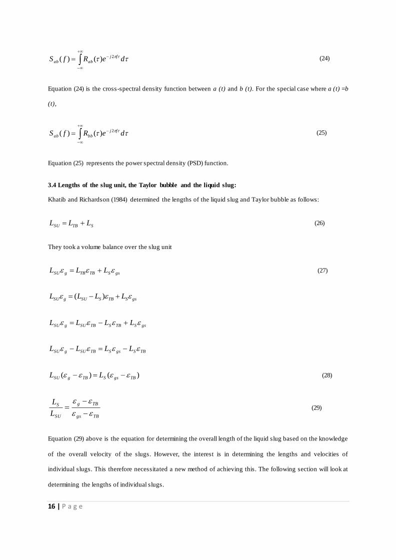
In Figure 20a, the Strouhal number based on the liquid superficial velocity is shown as a function of liquid

quality on a log-log plot. The liquid quality is defined as the ratio of liquid superficial velocity to mixture

superficial velocity.

Liquid quality,

SGSL

SL

UU

UX

(44)

The relationship between Strouhal number and the Lockhart -Martinelli parameter is shown in Figure 20b again

on a log-log plot. The Lockhart-Martinelli parameter is defined as the square root of the pressure drops for the

liquid part of the flow flowing alone in the pipe divided by that for the gas and it is approximately equal to the

ratio of liquid and gas superficial velocities times the square root of the liquid to gas density ratio (Abdulkadir

(2011)):

Lockhart-Martinelli parameter,

SG

SL

G

L

U

UX

(45)

Each plot exhibits a decrease in the Strouhal as the liquid quality or the Lockhart-Martinelli parameter increases.

Figure 20a shows the existence of three distinct regions of the Strouhal number for different values of the liquid

quality in the range 0.1<liquid quality< 0.5. The lower frequency Strouhal number is attributed to the large

scale instability of the liquid slug region. The higher frequency Strouhal number is caused by small scale

instabilities from the separation of the shear layer. The same trend can be observed for the variation of Strouhal

number with the Lockhart-Martinelli parameter as shown in Figure 20b.

35 | P a g e

Figure 20: Log-log plot of the dimensionless Strouhal number versus (a) the liquid quality (b) the Lockhart-

Martinelli parameter.

4.6 Lengths of the liquid slug, the Taylor bubble and the slug unit:

The lengths of the Taylor bubble and the slug unit are found to increase with a corresponding increase in the gas

superficial velocity, for a constant liquid superficial velocity as a parameter. It is observed that the lengths of the

Taylor bubbles and the slug units exhibit similar trends, showing a maximum stable length before a break up

(collapse). Therefore this suggests that the breakup could be a transition to churn flow as suggested by Hewitt

(1990).

36 | P a g e

Figure 21: Influence of gas superficial velocity on the ratio of average lengths of the liquid slug, Taylor bubble

and slug units to pipe diameter. The error bar represents standard deviation. These lengths were determined for

an experimental measurement averaging period of 60 seconds.

The average lengths of the liquid slugs as a function of the gas superficial velocity at various liquid flow rates

are shown on Figure 21(a). It can be concluded that there is no clearly defined trend for the variation of the

liquid slug with gas superficial velocity. However, it is interesting to note that at liquid superficial velocity of

0.38 m/s, the length of the liquid slug increases from approximately 6 to 9 pipe diameters and then decreases

finally to about approximately 6 pipe diameters. According to Moissis and Griffith (1962), the mean slug length

for the case of vertical pipe is almost in the range of 8 – 25 pipe diameters. The qualitative shape of the best fit

curve is a triangle, with a maximum at the top vertex. The stable liquid slug length is reported to be between 10

to 20 D (Moissis and Griffith (1962); Akagawa and Sakaguchi (1966); Fernandes (1981); Barnea and Shemer

(1989) and Van Hout et al. (2003)) for air-water system in a vertical pipe. The shorter liquid slug length

obtained may be attributed to the bigger pipe diameter used in the present experiments. It has been reported that

37 | P a g e

the slug flow pattern tends to disappear as the pipe diameter increases, Omebere-Iyari et al. (2008). A similar

trend is observed for a liquid superficial velocity of 0.14 m/s. For a particular flow condition, the length of the

slug is changing constantly due to the constant interaction between the phases at the tail of the Taylor bubble.

Consequently, different velocities can be obtained for individual Taylor bubbles .

From measured velocities and slug frequencies, the length of each Taylor bubble has been calculated. The

resulting lengths have been averaged for each gas and liquid superficial velocities. From an analysis of the data

presented on Figure 21(b) it is concluded that at certain liquid flow rates an almost linear relationship seems to

exist between the Taylor bubble length and the gas superficial velocity. Furthermore, an increase in the gas

superficial velocity leads to a proportional increase in Taylor bubble length. However, at a liquid superficial

velocity of 0.05 m/s, the length of the Taylor bubble is observed to increases from about 2 to 7 pipe diameter

and then to decrease to 6 pipe diameter. The increase in Taylor bubble length could be due to an increase in

bubble coalescence as a consequence of an increase in gas flow rate. The drop in length on the other hand at low

liquid flow rate may be due to the liquid entrainment into the Taylor bubble caused by waves and instabilities in

the liquid film surrounding the bubble as the gas flow rate is increased . This also results in the destruction of the

characteristic shape of the bubble.

The length of the slug unit on the other hand can be observed to increase with gas superficial velocity. But, it

can be observed that its length gets shorter with an increase in liquid superficial velocity. This is due to the fact

that frequency of slugging gets bigger with an increase in gas superficial velocity. A similar observation was

made by Hernandez-Perez (2008).

4.7 Comparison of Length of liquid slug with the Khatib and Richardson (1984) method:

A comparison between the experimental data and the Khatib and Richardson (1984) method for the length of

liquid slug has been made and is presented in Figure 22. The under-prediction of the Khatib and Richardson

method could be attributed to the simple empirically derived model they derived.

38 | P a g e

Figure 22: Comparison between the experimental data and the Khatib and Richardson (1984) method.

5. Conclusions

The paper has presented the experimental results to characterise the slug flow produced within a riser when

known quantities of air and silicone oil are injected at the base of the riser. The flow characteristics were

measured and characterised using non-intrusive instrumentation, including electrical capacitance tomography

(ECT) and a differential pressure transducer. That the following conclusions can be drawn:

(1) A linear relationship was obtained between structure velocity and mixture superficial velocity. A comparison

of this data with the empirical relationships proposed by Nicklin et al. (1962), Mao and Dukler (1985) and Hills

and Darton (1999) showed a qualitatively good agreement. The best quantitative agreement was obtained with

the relationship proposed by Hills and Darton (1976).

(2) The drift velocity according to the literature was developed by using potential flow analysis which assumes

no surface tension and viscosity effects on the drift velocity. The experimental results reveal that surface tension

and viscosity are significant parameters for drift velocity. Drift velocity for an air-silicone oil flow is higher for

that of air-water system.

(3) For a given liquid flow rate, as the gas flow rate was increased , the experimental average void fractions in

the liquid slug and the Taylor bubble were found to increase, while the liquid film thickness was found to

39 | P a g e

decrease. The liquid superficial velocity has an influence on the void fractions in the liquid slug and the Taylor

bubble. These findings were found to agree well with those made by previous published studies .

(4) The total pressure drop along the riser was found to decrease as the gas superficial v elocity increases, whilst

the measured frictional pressure drop was found to increase.

(5) The slug frequency increased with an increase in the liquid superficial velocity, whilst the dimensionless

Strouhal number was found to decrease with corresponding increases in the liquid quality and the Lockhart-

Martinelli parameter. The manual counting method for the determination of slug frequency was found to be

satisfactory when a threshold value of 0.3 for void fraction was used as suggested by Nydal (1991). The

Hernandez-Perez et al. (2010) correlation gave the best agreement with experimental data.

(6) The dimensionless lengths of the liquid slugs, the Taylor bubbles, and the slug units were found to increase

with an increase in the gas superficial velocity. However, the length of the liquid slug was found change due to a

coalescence of the dispersed bubbles from the wake of a Taylor bubble with the Taylor bubble. This is in

agreement with the result obtained by Akagawa and Sakaguchi (1966); Fernandes (1981) an d Van Hout et al.

(2002)

(7) An adequate agreement was found between the experimental liquid slug length and the Khatib and

Richardson method (1984) after considering the influence of the void fraction in liquid slug.

This study has provided a more fundamental insight into the physical phenomena that govern the behaviour of

slug flows and the way these parameters behave under various flow conditions.

7. Nomenclature

Symbol Description, Units

0C Distribution coefficient, dimensionless

D

f

Pipe diameter, m

Frequency, Hz

g Gravity constant, 9.81 m/s2

MU Mixture superficial velocity, m/s

NU Structure velocity or nose velocity of a Taylor bubble, m/s

SGU Gas superficial velocity, m/s

SLU Liquid superficial velocity, m/s

GLSU Gas superficial velocity in liquid slug, m/s

LLSU Liquid superficial velocity in liquid slug, m/s

40 | P a g e

0U Terminal velocity of a bubble rising through fluid, m/s

x Liquid quality,

SGSL

SL

UU

Ux

Greek Symbols

ab

Density, 3/ mkg

Population correlation coefficient

ba ,

Viscosity, mskg /

Mean of the corresponding series

Surface tension, mN /

NU Increment of UST as defined in equation (1), m/s

L

P

Pressure drop, mN /

gs Void fraction in liquid slug, dimensionless

TB Void fraction in Taylor bubble, dimensionless

Liquid film thickness, mm

Ratio of void fraction in liquid slug and Taylor bubble, dimensionless

g

E

)(abR

Mean void fraction, dimensionless

Expected value operator

Cross-correlation function between a (t) and b (t)

Subscripts

G Gas phase

L Liquid phase

LLS Liquid in liquid slug

GLS Gas in liquid slug

s Slug

M Mixture

Dimensionless numbers

Eo Eotvos number,

gDEo

2

Fr

Mo

Froude Number, Frm=Um2/Gd

Morton number, Mo =3

4

g

fN Dimensionless inverse viscosity number,

4/1

0

3

0

M

EN f

41 | P a g e

X Lockhart-Martinelli parameter,

G

L

L

P

L

P

X

St

Strouhal Number,

SLU

FDSt

ACKNOWLEDGEMENTS

M. Abdulkadir would like to express sincere appreciation to the Nigerian government through the Petroleum

Technology Development Fund (PTDF) for providing the funding for his doctoral studies.

This work has been undertaken within the Joint Project on Transient Multiphase Flows and Flow Assurance,

sponsored by the UK Engineering and Physical Sciences Research Council (EPSRC); Advantica; BP

Exploration; CD-adapco; Chevron; ConocoPhillips; ENI; ExxonMobil; FEESA; IFP; Institutt for Energiteknikk;

Norsk Hydro; PDVSA (INTERVEP); Petrobras; PETRONAS; Scandpower PT; Shell; SINTEF; Statoil and

TOTAL. The Authors wish to express their sincere gratitude for their supports.

References

Abdulkadir, M., 2011. Experimental and computational fluid dynamics (CFD) studies of gas -liquid flow in bends.

PhD Thesis, University of Nottingham

Abdulkadir, M., Zhao, D., Sharaf, S., Abdulkareem, L., Lowndes, I.S., and Azzopardi, B. J., 2011. Interrogating the

effect of 90o bends on air-silicone oil flows using advanced instrumentation. Chemical Engineering Science, 66,

2453 - 2467.

Abdulkadir, M., Hernandez-Perez, V., Sharaf, S., Lowndes, I. S. & Azzopardi, B. J., 2010. Experimental

investigation of phase distributions of an air-silicone oil flow in a vertical pipe. World Academy of Science,

Engineering and Technology, 61, 52 – 59

Akagawa, K., and Sakaguchi, T., 1966. Fluctuation of void fraction in gas -liquid two-phase flow. Bulletin JSME, 9,

104-110

Azzopardi, B. J., 1997. Drops in annular two-phase flow. International Journal of Multiphase Flow 23, S1 - S53.

Azzopardi, B. J., Abdulkareem, L.A., Sharaf, S., Abdulkadir, M., Hernandez-Perez, V., &.Ijioma, A., 2010. Using

tomography to interrogate gas-liquid flow. In: 28th UIT Heat Transfer Congress, Brescia, Italy, 21 - 23 June.

Barnea, D. and Shemer, L., 1989. Void fraction measurements in vertical slug flow: applications to slug

characteristics and transition. International Journal of Multiphase Flow, 15, 495 - 504.

Barnea, D., and Taitel, Y., 1993. A model for slug length distribution in gas -liquid slug flow. International Journal

of of Multiphase flow, 19,829 - 838.

Bendat, J., and Piersol, A., 1980. Engineering application of correlation and spectral analysis. John Wiley and Sons,

New York, USA.

42 | P a g e

Brauner, N., and Ullmann, A., 2004. Modelling of gas entrainment from Taylor bubbles, Part A: Slug flow,

International Journal of Multiphase flow, 30, 239 - 272.

Brown, R. A. S., 1965. The mechanics of large gas bubbles in tubes: I. Bubble velocities in stagnant liquids.

Canadian Journal of Chemical Engineering, 43, 217 - 223

Costigan, G., and Whalley, P. B., 1996, Slug flow regime identification from dynamic void fraction measurements

in vertical air-water flows. International Journal of Multiphase Flow, 23, 263 - 282

Collins, R., De Moraes, F. F., Davidson, J. F., and Harrison, D., 1978. The motion of a large gas bubble rising

through liquid flowing in a tube. Journal of Fluid Mechanics, 89, 497 - 514.

da Silva, M.J., Thiele, S., Abdulkareem, L., Azzopardi, B.J., Hampel, U., 2010, High-resolution gas-oil two-phase

flow visualization with a capacitance wire-mesh sensor. Flow Measurement and Instrumentation, 21,191 - 197.

Davies, R.M. and Taylor, G.I., 1950. The mechanics of large bubbles rising through extended liquids and through

liquids in tubes. Proceedings of the Royal Society, A 200, 375 - 395

Dumitrescu, D. T. 1943. Stromung an einer luftblase in senkrechten rohr Z angrew Math Mech , 23, 139 - 149

de Chard, F. and Delhaye, J. M., 1996. A slug-churn flow model for small-diameter airlift pumps. International

Journal of Multiphase Flow, 22, 627 - 649.

Fabre, J., and Line, A., 1992. Modelling of two-phase slug flow. Annual Review of Fluid Mechanics, 24, 21- 46

Fernandes, R. C., Semiat, R., and Dukler, A.E., 1983. Hydrodynamics model for gas -liquid slug flow in vertical

tubes. AIChE Journal, 29, 981 - 989

Geraci, G., Azzopardi, B. J., and Van Maanen, H. R. E., 2007a. Inclination effects on circumferential film

distribution in annular gas/ liquid flows. AIChE Journal, 53, 1144 - 1150.

Geraci, G., Azzopardi, B. J., and Van Maanen, H. R. E., 2007b. Effects of inclination on circumferential film

thickness variation in annular gas/ liquid flows . Chemical Engineering Science, 62, 3032 - 3042.

Godbole, S. P., Honath, M. F., and Shah, Y. T., 1982. Holdup structure in highly viscous Newtonian and non-

Newtonian liquids in bubbles . Chemical Engineering Communications, 16, 119 - 134.

Gregory, G. A., and Scott, D.S., 1969. Correlation of liquid slug velocity and frequency in horizontal co-current

gas-liquid slug flow. AIChE Journal, 15, 833 - 835.

Griffith, P., and Wallis, G. B., 1961. Two-phase slug flow. Journal of Heat Transfer, 83, 307 - 320.

Friedel, L., 1980. Pressure drop during gas/vapour-liquid flow in pipes. Int. Chem Engineering, 20, 352 - 367.

Hammer, E. A., 1983.Three-component flow measurement in oil/gas/water mixtures using capacitance transducers .

PhD thesis, University of Manchester

Hernandez-Perez, V., 2008. Gas-liquid two-phase flow in inclined pipes. PhD thesis, University of Nottingham.

Hernandez-Perez V, Abdulkadir M., and Azzopardi B. J., 2010. Slugging frequency correlation for

inclined gas-liquid flow. World Academy of Science, Engineering and Technology, 61, 44 – 51.

Hewitt G. F., 1990. Non-equilibrium two-phase flow. In: 9th International Heat Transfer Conference, Jerusalem, 1,

383 - 394.

Hills, J.H., and Darton, R.C., 1976. Rising velocity of large bubble in a bubble swarm. Trans I. Chem. Engrs, 54,

258 – 264.

Holman, J.P., 1994. Experimental methods for engineers, 6th edn, McGraw-Hill Inc, New York

Huang, S. M., 1995. Impedance sensors-dielectric systems. In R.A. Williams, and M. S. Beck (Eds.). Process

Tomography, Cornwall: Butterworth-Heinemann Ltd.

43 | P a g e

Hubbard, M. G., 1965. An analysis of horizontal gas-liquid slug. PhD Thesis, University of Houston, Houston,

USA

Jepson, W. P., and Taylor, R. E., 1993. Slug flow and its transition in large diameter horizontal pipes . International

Journal of Multiphase flow, 19, 411 - 420.

Kaul, A., 1996. Study of slug flow characteristics and performance of corrosion inhibitors in multiphase flow in

horizontal oil and gas pipelines. PhD Thesis, Ohio University.

Khatib, Z., and Richardson, J. F., 1984. Vertical co-current flow of air and shear thinning suspensions of kaolin.

Chemical Engineering Research and Design, 62,139 - 154

Liu, J.J., 1993. Bubble size and entrance length effects on void development in a vertical channel. International

Journal of Multiphase flow, 19, 99 - 113.

Mahalingam, R., and Valle, M., 1972.Momentum transfer in two-phase of gas-pseudoplastic liquid mixtures .

Industrial and Engineering Chemistry Fundamentals, 11, 470 - 477.

Mandal, A., Kundu, G., and Mukherjee, D., 2004. Studies on frictional pressure drop of gas -non-Newtonian two-

phase flow in a co-current downflow bubble column. Chemical Engineering Science, 59, 3807 - 3815

Manolis, I. G., Mendes-Tatsis, M.A., and Hewitt, G. F., 1995. The effect of pressure on slug frequency on two-

phase horizontal flow. In: 2nd International Conference on Multiphase flow, Kyoto, Japan, April 3 - 7

Mao, Z. S., and Dukler, A.E., 1985. Brief communication: Rise velocity of a Taylor bubble in a train of such

bubbles in a flowing liquid. Chemical Engineering Science, 40, 2158 - 2160

Moissis, R.,1963. The transition from slug to homogeneous two-phase flows. ASME Journal of Heat Transfer, 29 -

39

Moissis, R., and Griffith, P., 1962. Entrance effects in two-phase slug flow. ASME Journal of Heat Transfer, 366 -

370

Mori, K., Kaji, M., Miwa, M., and Sakaguchi, K., 1999. Interfacial structure and void fraction of liquid slug for

upward gas-liquid two-phase slug flow. Two Phase Flow Modelling and Experimentation, Edizioni ETS, Pisa

Nicklin, D. J., Wilkes, J. O., and Davidson, J. F., 1962. Two-phase flow in vertical tubes. Transaction of Institution

of Chemical Engineers, 40, 61- 68

Nydal, O.J., 1991. An experimental investigation of slug flow. PhD Thesis, University of Oslo

Omebere-Iyari, N. K., Azzopardi, B. J., Lucas, D., Beyer, M., Prasser, H.-M., 2008. The characteristics of

gas/liquid flow in large risers at high pressures. International Journal of Multiphase Flow, 34, 461 - 476.

Sylvester, N.D., 1987. A mechanistic model for two-phase vertical slug flow in pipes . Journal of Energy Resource

Technology, 109, 206 - 213.

Ros, N. C. J., 1961. Simultaneous flow of gas and liquid as encountered in well tubing . Journal of Petroleum

Technology, 13, 1037 - 1049.

Taitel, Y., and Dukler, A.E., 1977. A model for slug frequency during gas -liquid flow in horizontal and near

horizontal pipe. International Journal of Multiphase flow, 3, 47 - 55

Taylor, G. I., 1961. Disposition of a viscous fluid on the wall of a tube, Part ii. Journal of Fluid Mechanics, 10, 161

Van Houst, R., Barnea, D., and Shemer, L., 2002. Translational velocities of elongated bubbles in continuous slug

flow. International Journal of Multiphase flow, 28, 1333 - 1350.

Vince, M. A., and Lahey, R. T., 1982. On the development of an objective flow regime indicator. International

Journal of Multiphase flow, 8, 93 - 124.

44 | P a g e

Wallis, G. R., 1969. One- dimensional two-phase flow. McGraw-Hill, New York

White, E. T. and Beardmore, R. H., 1962. The velocity of rise of single cylindrical air bubbles through liquids

contained in vertical tubes . Chemical Engineering Science, 17, 351 - 361.

Zabaras, G.J., 1999. Prediction of slug frequency for gas/liquid flows. Society of Petroleum Engineers

(SPE), 5, 252 – 258.

Zhu, K., Madhusudana Rao, S., Wang, C., and Sundaresan, S., 2003. Electrical capacitance tomography

measurements on vertical and inclined pneumatic conveying of granular solids . Chemical Engineering Science, 58,

4225 - 4245.

Zoeteweij, M.L., 2007. Long liquid slugs in horizontal tubes: development study and characterisation with electrical

conductance techniques . PhD thesis, Delft University of Technology, Netherlands.

45 | P a g e

Figure captions:

Figure 1 A schematic diagram of the riser rig

Figure 2 The electrical capacitance tomography (ECT) sensor

Figure 3 Gas-liquid mixing section

Figure 4 Void fraction time series from the two ECT probes

Figure 5 Shoham (2006) flow pattern map showing experimental data points

Figure 6 Time trace of void fraction showing liquid slug, Taylor bubble and slug unit

Figure 7 PDF of cross-sectional average void fraction for the case of slug flow measured from the experiments

using air-silicone oil

Figure 8 Comparison of 3-D plot of PDFs of void fraction obtained from the (a) ECT and (b) WMS. Liquid

superficial velocity = 0.05 m/s

Figure 9 Experimentally measured structure velocity vs mixture velocity

Figure 10 Experimentally measured structure velocity, Nicklin et al. (1962) and Darton (1976) correlations

against mixture superficial velocity

Figure 11 Comparison between the experimental data and the considered empirical correlations

Figure 12 The determined mean gas void fractions in the (a) liquid slug (b) Taylor bubbles (c) liquid film

thickness

Figure 13 A plot of the relationship between the void fraction in the liquid slug and the mean void fraction

Figure 14 The influence of the gas superficial velocity on the total and frictional pressure drop

Figure 15 Variation of slug frequency with gas superficial velocity at different liquid superficial velocity

Figure 16 Threshold of the void fraction used in counting slugs

Figure 17 Plot of slug frequency determined from the manual counting method against PSD computed method

Figure 18 Variation of slug frequency with gas superficial velocity using results obtained from experiments

and empirical correlations at liquid superficial velocity of (a) 0.05 m/s (b) 0.09 m/s (c) 0.28 m/s and (d) 0.38 m/s

Figure 19 Comparison between the experimental data and the considered empirical correlations

46 | P a g e

Figure 20 Log-log plot of the dimensionless Strouhal number vs (a) the liquid quality (b) the Lockhart-

Martinelli parameter

Figure 21 Influence of gas superficial velocity on the ratio of average lengths of the liquid slug, Taylor bubble

and slug units to pipe diameter

Figure 22 Comparison between the experimental data and the Khatib and Richardson method (1984)

47 | P a g e

Table captions:

Table 1 Properties of the fluids and dimensionless numbers at1 bar and at the operating temperature of

5.020 oC

Table 2 Table of the flowchart for experimental measurement used to obtain the parametrical characterisation

of the slug flow regime

Table 3 Measurement uncertainties