NBER WORKING PAPER SERIES

FERTILITY, FEMALE LABOR FORCE PARTICIPATION, AND THE DEMOGRAPHICDIVIDEND

David E. BloomDavid CanningGünther Fink

Jocelyn E. Finlay

Working Paper 13583http://www.nber.org/papers/w13583

NATIONAL BUREAU OF ECONOMIC RESEARCH1050 Massachusetts Avenue

Cambridge, MA 02138November 2007

The authors are grateful to David Weil and the participants of the Workshop on Population Agingand Economic Growth for their valuable comments. We extend our thanks to Mansour Farahani forcompiling the family planning data. Support for this research was provided by grant number 5 P30AG024409 from the National Institute on Aging, National Institutes of Health, and by grants fromthe William and Flora Hewlett Foundation and the John D. and Catherine T. MacArthur Foundation.The views expressed herein are those of the author(s) and do not necessarily reflect the views of theNational Bureau of Economic Research.

�© 2007 by David E. Bloom, David Canning, Günther Fink, and Jocelyn E. Finlay. All rights reserved.Short sections of text, not to exceed two paragraphs, may be quoted without explicit permission providedthat full credit, including �© notice, is given to the source.

Fertility, Female Labor Force Participation, and the Demographic DividendDavid E. Bloom, David Canning, Günther Fink, and Jocelyn E. FinlayNBER Working Paper No. 13583November 2007JEL No. J01,J1,J13,J21

ABSTRACT

We estimate the effect of fertility on female labor force participation in a cross-country panel dataset using abortion legislation as an instrument for fertility. We find a large negative effect of the fertilityrate on female labor force participation. The direct effect is concentrated among those aged 20-39,but we find that cohort participation is persistent over time giving an effect among older women. Wepresent a simulation model of the effect of fertility reduction on income per capita, taking into accountthese changes in female labor force participation as well as population numbers and age structure.

David E. BloomHarvard UniversityDepartment of Populationand International HealthBuilding I655 Huntington Ave.Boston, MA 02115and NBERdbloom@hsph.harvard.edu

David CanningHarvard School of Public HealthSPH Population International HealthSPH1 1211677 Huntington AvenueBoston, MA 02115dcanning@hsph.harvard.edu

Günther FinkHarvard School of Public HealthHarvard Universitygfink@hsph.harvard.edu

Jocelyn E. FinlayHarvard School of Public HealthHarvard Universityjfinlay@hsph.harvard.edu

1. Introduction

During the demographic transition, sharp declines in fertility lead to large changes

in a population’s age structure. Smaller birth cohorts decrease youth dependency ratios

and mechanically increase output per capita if output per worker and the labor force

participation rate of the working-age population remain unchanged. This generates the

demographic dividend, which has been shown to be important in explaining cross-

country variation in the growth of per capita income (Bloom and Freeman 1987; Brander

and Dowrick 1994; Kelley and Schmidt 1995; Bloom and Williamson 1998; Bloom,

Canning et al. 2003).

In addition to creating these age structure effects, demographic change may also

incite behavioral changes. Longer life spans may affect retirement and savings decisions

(Bloom, Canning et al. 2007), while fertility reduction can affect female labor market

participation. We use a panel of 97 countries over the period 1960 to 2000 to examine the

effect of fertility on female labor force participation by five-year age groups.

Studies of the impact of fertility are complicated by the endogeneity of fertility

and the resulting difficulty in identifying the direction of causality (Browning 1992). In

microeconomic studies it is common to use twins, or the sex composition of previous

births, as factors that produce exogenous variation in fertility (e.g., Rosenzweig and

Wolpin 1980; Angrist and Evans 1998). Changes in legislation have also been used as

instruments for fertility. Levine, Staiger, Kane and Zimmerman (1999) and Klerman

(1999) find that the legalization of abortion in the United States led to a decrease in

fertility. Angrist and Evans (1996) find that state-level legalization of abortion reduced

fertility and increased the labor force participation of black women. Bailey (2006) uses

state-level variations in contraceptive pill legislation as an instrument for fertility, and

finds an effect of fertility on labor force participation.

In our analysis we use country level abortion legislation as an instrument for

fertility. Henshaw, Singh and Haas (1999) estimate that worldwide around 26 percent of

pregnancies end in abortion, making it a common method of avoiding childbirth.

2

Although the precise timing of abortion laws may be considered random, this type of

liberal legislation may reflect broader trends in society that are also correlated with

female labor market participation. We control for these social factors by including both

country fixed effects and country-specific time trends in our analysis.

Mammen and Paxson (2000), expanding on work by Goldin (1995), find the

relationship between female participation rates and per capita income to be U-shaped. In

poor, agricultural economies, female participation is high as family responsibilities and

agricultural work can easily be combined. Female participation is lowest in urbanized,

middle-income countries that are dominated by a manufacturing sector. Low levels of

female education, the income effect of male earnings, and the separation of home and

work environments contribute to lower participation rates. Female participation rates are

again high in high-income countries with large service sectors and highly educated

women. This reflects the role of urbanization in female labor force participation, which

we control for in our analysis.

Our empirical results imply that the effect of fertility on female labor supply is

strongest during the fertile years (20–39 years of age). We find a high degree of

persistence in labor market participation, so that higher total fertility is associated with

lower female labor force participation even at older ages. On average, our results imply

that with each additional child, female labor force participation decreases by about 10–15

percentage points in the age group 25–39, and about 5–10 percentage points in the age

group 40–49. These results imply a reduction of about four years of paid work over a

woman’s lifetime for each birth.

To illustrate the growth effects of the demographic transition with endogenous

labor supply, we simulate long-run income dynamics using a simple production function

model. We calibrate the model using data for South Korea, which saw a reduction in its

total fertility rate from 5.6 children per woman in 1962 to 1.2 in 2002. The decline in

fertility has three main effects. First, lower fertility implies lower population growth, and

thus increases the capital-to-labor ratio in the standard Solow model. In our simulations,

3

this effect leads to an increase in per capita income of about 36 percent over the period.

Second, the fertility reduction increases the ratio of working-age population to total

population by lowering the youth dependency ratio. Keeping age- and sex-specific

participation rates steady at their 1960 levels, this age structure effect raises the relative

size of the labor force, leading to a 47 percent increase in per capita income. Third, the

fertility reduction increases female labor force participation. Using our point estimates

from the empirical section, we find that the increase in female labor force participation

generates a further gain in income per capita of 21 percent.

The combination of these effects2 implies an increase in income per capita by a

factor of around 2.4. Although this is only a portion of the almost eleven-fold rise in

income per capita that South Korea saw over the period, the reduction in fertility and

increase in labor supply per capita may help explain this apparent growth “miracle”

(Bloom, Canning et al. 2000). Although labor supply per capita is bounded above, and so

cannot affect the rate of economic growth in the very long run, it can give a substantial

boost to growth over a medium period of fifty years. If the transition from high fertility to

low fertility is permanent, then there are long-run effects on age structure and persistent

effects on female labor supply, and the gains in income per capita may be permanent.

A common finding in the empirical growth literature is that there is little

relationship between the rate of population growth and the rate of growth of income per

capita (see, e.g., Simon 1989). Our results do not invalidate this. We argue that a decline

in population growth associated with a decrease in fertility can produce economic

growth. However, if slow rates of population growth are due to ill health and high

mortality, positive growth effects do not yield. Even though population growth has little

correlation with economic growth, fertility and mortality rates considered separately

appear to have large effects (Bloom and Freeman 1987; Kelley and Schmidt 1995).

2 The effects are roughly multiplicative, even though the labor supply effects tend to reduce the capital/labor ratio somewhat.

4

This paper is structured as follows: in section two, we present a model of labor

supply and fertility. In section three, we present the data, and in section four, we discuss

abortion legislation as an instrument for fertility. In section five we present the empirical

results, and in section six, we discuss our simulation framework and show the simulation

results of the medium-run effects of fertility decline on per capita income. We conclude

with a summary and discussion.

2. Model

We propose a simple model of female fertility and labor supply choices. The

utility function U for a representative woman is defined over consumption c, leisure d,

and fertility n. It is assumed to be given by:

( ) ( ) ( )0( , , ) log log log log NU c d n c c d n kn

α β ⎛ ⎞= + + + − ⎜ ⎟⎝ ⎠

(1.1)

For simplicity we assume a logarithmic functional form. The weight on consumption is

normalized to 1. The relative weight of leisure in utility is 0α > , while the relative

weight given to children is 0.β > We might think of 0c as being negative and

representing subsistence consumption. Alternatively, 0c might be taken to be positive and

reflect transfers from a working husband to the woman. In addition to the utility of

children, we assume there is a psychological cost k of avoiding childbirth and achieving

fertility lower than N, the potential reproductive capacity (or fecundity rate), usually

taken to be around 15 on average. Obviously, actual fertility is usually regulated to be

lower than this maximum. This regulation usually takes the form of delayed marriage,

contraceptive use, abortion, or postpartum insusceptibility due to abstinence and

breastfeeding after birth (Bongaarts 1984).

Total time available is normalized to one. This is divided between working time l,

leisure time d, child care bn and other non-market household work ε . That is,

1 l d bn ε= + + + (1.2)

The time allocated to child care is assumed to be linear in the number of children,

with a time cost per child b. We assume 0b > and 0 1ε≤ < . A woman's consumption

5

possibilities are limited by the amount of income she earns: the prevailing wage w times

the amount of time she spends working l. All income earned is consumed, and the

consumption constraint is defined as

c wl= (1.3)

We assume 0(1 ) 0w cε− + > , so that consumption above the subsistence level is

feasible. We treat constraints (1.2) and (1.3) as binding; if they are regarded as inequality

constraints the fact that consumption and leisure time are always desirable will make

them binding under maximization. Given these time allocation and consumption

constraints we can write utility as a function of labor supply and the number of children:

( ) ( ) ( ) ( )0, log log 1 log log NV n l wl c l bn n kn

α ε β ⎛ ⎞= + + − − − + − ⎜ ⎟⎝ ⎠

(1.4)

where 0 n N≤ ≤ and 0 1l≤ ≤ .

The first order conditions for an interior maximum with respect to l and n are:

0

01

dV wdl wl c l bn

αε

= − =+ − − −

(1.5)

01

dV k bdn n n l bn

β αε

= + − =− − −

(1.6)

In Appendix A we show that the Hessian matrix is negative semi-definite, which implies

that the first-order conditions above generate a local maximum. Given a fixed number of

children n the optimal labor supply is given by

01 1 ,1

cl bnwα ε

α⎛ ⎞= − − −⎜ ⎟+ ⎝ ⎠

(1.7)

while given a fixed labor supply l the optimal number of children is

( ) ( )1 .kn l

b kβ ε

α β+

= − −+ +

(1.8)

We wish to estimate the structural equation (1.7) to find the effect of variations in

fertility on female labor supply. The optimal labor supply is decreasing in fertility and the

6

slope of the relationship depends on the time cost of children and the relative weights of

consumption and leisure in utility. There is a possibility that the time required by other

non-market household work ε is random and not observed, which will create an error

term in the estimation of equation (1.7). However, the non-market work time required

also affects fertility in equation (1.8). Both fertility and labor supply are thus jointly

determined and the parameters of equation (1.7) will not be identified in a simple

regression. However, solving equations (1.7) and (1.8) for fertility we have

( ) ( )( )

( )0 1

* ,1

k c wn

bw kβ ε

α β+ + −

=+ + +

(1.9)

and

( )( )( )

( )0

2

1 1* 0.1

c wdndk bw k

ε α

α β

+ − += >

+ + + (1.10)

This implies that optimal fertility is high when the cost of fertility control is high. The

cost of fertility control is correlated with the fertility decision, but is not correlated with

the error term in labor supply given by equation (1.7). The cost of fertility control affects

labor supply only through its effect on the level of fertility. It follows that the cost of

fertility control can be used as an instrument for fertility in estimating equation (1.7).

The wage rate affects both fertility and labor supply. The effect depends on the

balance of income and substitution effects. If 0 0c > , the substitution effect dominates,

and, conditional on fertility, labor supply is rising with female wages. On the other hand,

if 0 0c < , the income effect dominates, and for a given fertility female labor supply is

declining in the wage rate.

We estimate the causal negative effect of fertility on labor supply, holding

everything else constant, as given by equation (1.7). Note, however, that fertility and

labor supply can rise together if some of the parameters in our model change. For

example, a decrease in ε , the time required for non-child related work in the home, can

increase both fertility and female labor supply, which is consistent with the positive

7

correlation between female labor supply and fertility in OECD countries found by

Engelhardt and Prskawetz (2004).

3. Data

The data set we use in our empirical work is an unbalanced five-year panel

covering the period from 1960 to 2000 for 97 countries.3 The dependent variable in our

empirical analysis is female labor force participation. Labor market participation data are

taken from the International Labor Organization (2007) and cover all age groups between

15–19 years old and 60–64 years old in five-year age increments. The International Labor

Organization (ILO) data are based on national labor market surveys and censuses. The

female participation rate is the number of economically active women divided by the

total female population in the same age group. Although definitions vary slightly across

countries, a woman is classified as “economically active” if she is either employed or

actively looking for work (ILO Bureau of Statistics 2007).

Our explanatory variables are the fertility rate, the percentage of the population

living in urban areas, physical capital per working-age person, female life expectancy and

the average years of schooling of men and women. We use the stock of physical capital

per working-age person, female life expectancy and the education level of women as a

proxy for the wage rate. The education level of men serves as a proxy for male income

and intra-family transfers, even though male education may also directly affect female

wages if male and female human capital are substitutes.

Total fertility rates, female life expectancy and urbanization rates are from the

World Development Indicators (World Bank 2006). The physical capital stock is from

the Penn World Tables 6.2 (Heston, Summers et al. 2006), deflated by the working-age

population rather than the number of workers as would be more usual, to avoid potential

simultaneity biases in our estimation. Our human capital measures are the average years

3 For a full list of countries, please see Appendix Table A2.

8

of schooling in the female and male population aged 15 and older, respectively, as

measured by Barro and Lee (2000).

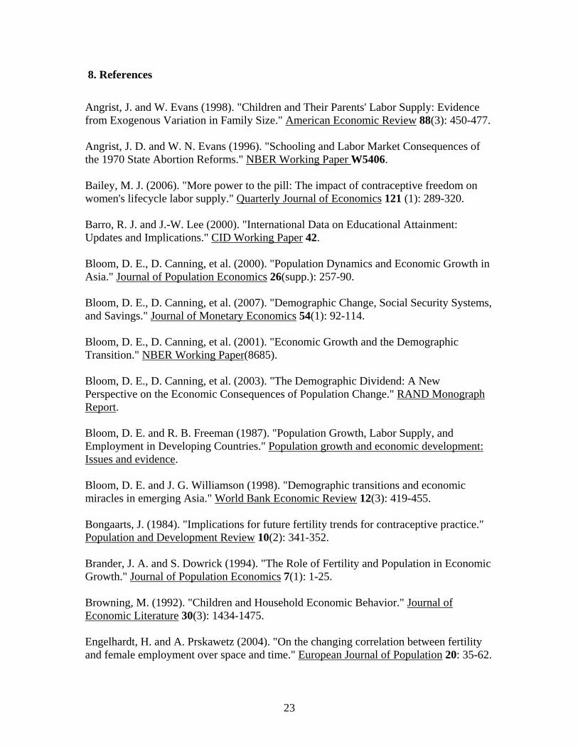
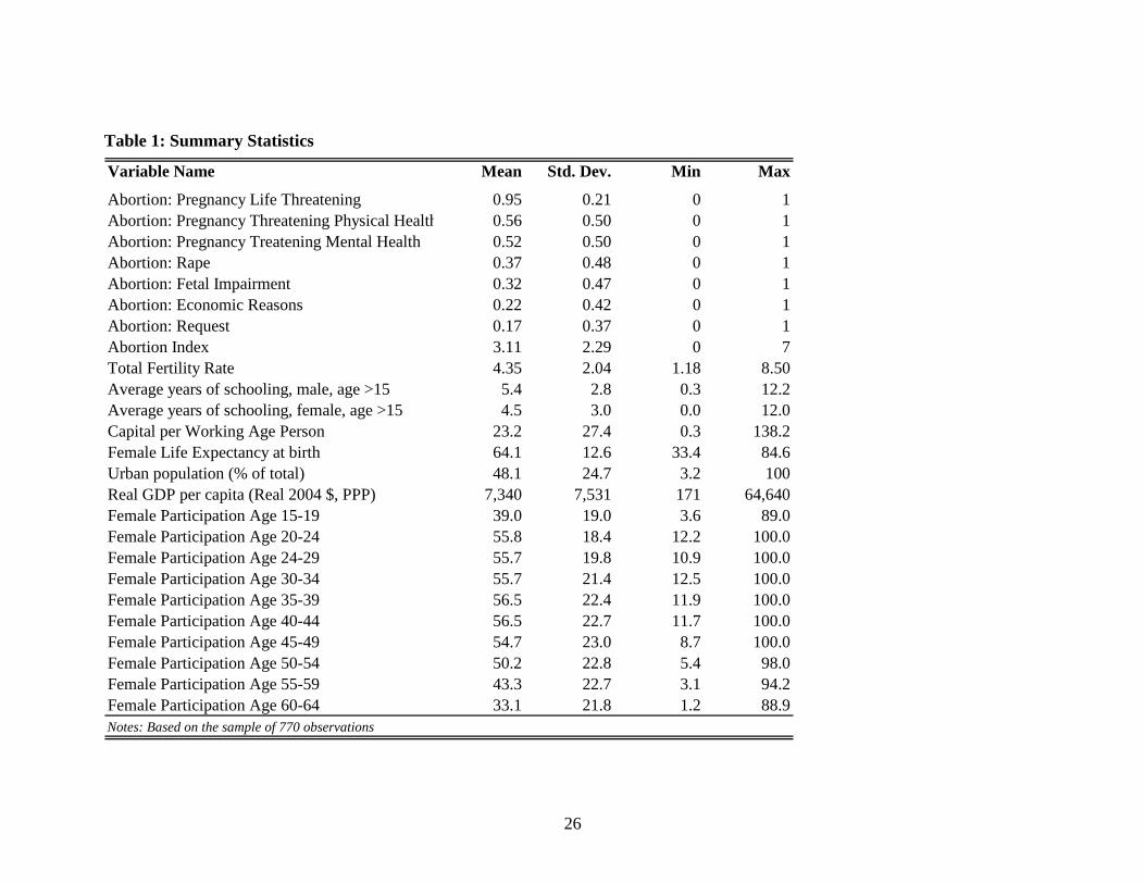
Table 1 provides summary statistics for our main variables; a more detailed

description of the data and data sources is provided in Appendix Table A1. The total

fertility rate ranges from 1.18 (Spain and Italy in 1995) to 8.5 (Rwanda in 1980), with an

average in the panel of 4.35. The average female labor force participation shows little

variation across age groups, but great variation across countries for each age group.

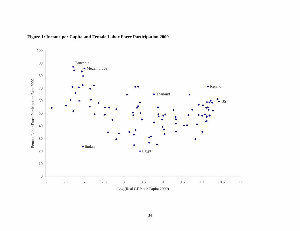
Figure 1 shows average female participation rates for women aged 15–64 in 2000. These

range from values close to 90 percent in Tanzania and Mozambique to only 20 percent in

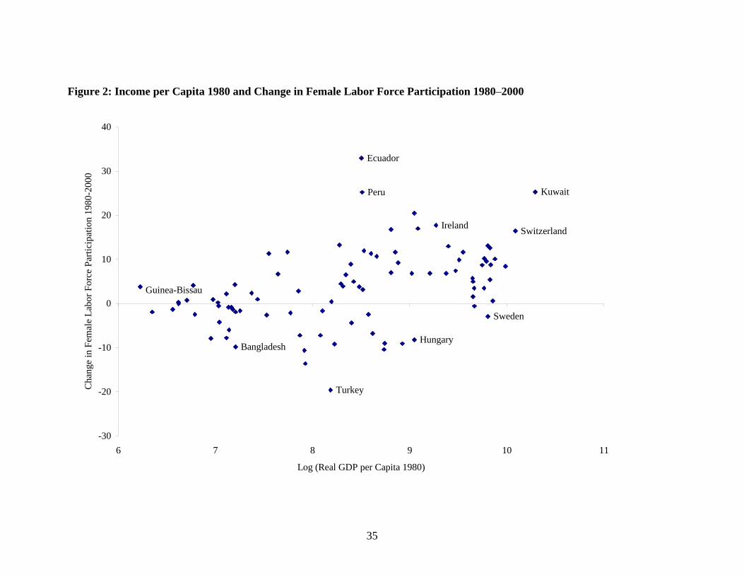
Egypt, and show a pronounced U-shape. Figure 2 shows the change in participation over

the period 1980 to 2000. Although a general increase in female labor force participation

is visible in the data, and particularly pronounced in high-income countries, there is

sizable variation in participation rates, ranging from an increase of more than 25 percent

in Ecuador, Peru and Kuwait to a decrease of nearly 20 percent in Turkey.

[Table 1]

4. Abortion Legislation as an Instrument for Fertility

To construct an instrument for fertility we use data on national abortion

legislation compiled by the United Nations Population Division (United Nations

Population Division 2002). The data contain detailed information on the availability of

abortion over time.4 We use the United Nations system to classify the laws in place. The

United Nations system classifies seven legal reasons for an abortion: to save the life of

the woman; to preserve her physical health; to preserve her mental health; consequent on

rape or incest; fetal impairment; economic or social reasons; and available on request.

Our data contain indicator variables for each of these seven categories. A “1” indicates

that abortion is available for the given reason, and “0” means that it is not. When an

abortion is available on request, we assume availability for any of the other reasons if this

is not explicitly stated.

4 We are grateful to Mansour Farahani for compiling the data.

9

Although these categories are broad, they are not comprehensive descriptions of

abortion law. There are frequently cutoffs for lawful abortions depending on the length of

the pregnancy. The mechanisms for adjudicating if a pregnancy meets a particular

criterion differs across countries, relying in some cases on a single doctor, while in others

two are more doctors are required to agree. In some countries a husband's consent is

required. The United Nation coding scheme ignores these additional factors and declares

an abortion for a particular reason lawful if it is allowed at any time during the

pregnancy. In federal systems, abortion laws sometimes differ across regions. In this case

the law that covers the majority of the population, if one exists, is used to classify at the

national level.

We use the values of these variables as coded by the United Nations to provide a

value for the most recent year at which data are available. For earlier years we recode the

variable to reflect a country's legal situation at a given time as set out in the United

Nations documentation of abortion legislation history. This recoding is complicated by

the need to consider not only statutes that relate to abortion, but also the evolution of case

law in the interpretation of those statutes.

In many countries there is a divergence between law and practice, with abortions

being widely available despite being technically illegal, or vice versa. We take the

objective stance and code according to the law. For example, in the United Kingdom

(excluding Northern Ireland) the Abortion Act of 1967 allows abortion to protect the life,

physical and mental health of the mother, and in cases where there is a risk the child will

be handicapped. The law also covers cases where a birth might affect the health of

existing children and allows the woman's actual and potential environment to be taken

into account. Legally, abortion is not explicitly available in the case of rape or simply on

request. Although this is the legally restricted set of criteria, in practice the physical and

mental health criteria appear to be interpreted liberally. They include the effects of

childbirth on socio-economic circumstances and hence health outcomes so that de facto

an abortion is available if a woman requests one. In the case of rape a claim that abortion

10

was needed to preserve the mental and physical health of the mother would be very likely

to succeed (as in the case of Rex v. Bourne, 1938). A second example is Chile. The law

of 1874 prohibited abortions carried out with malice; it was understood that abortions to

save the life of the mother were permitted. This was explicitly recognized in the law of

1967. The law was changed in 1989 to outlaw abortions in all circumstances (though

some commentators suggest that a defense of necessity to save the life of the mother

would succeed). Despite these strict laws, abortion has been relatively common in Chile

throughout the period. We code Chile as allowing abortion to save the life of the mother

from 1960 to 1988 and as not allowing abortion under any circumstances thereafter.

Table 1 summarizes the abortion data. The “life threatening” indicator has an

average of 0.95, which implies that almost all countries across the sample period allow

abortion under this circumstance. There is more variation across countries and time for

the availability of abortion on the remaining categories. We construct an index

summarizing the availability of abortion. A country gets a score of zero if abortion is not

legal for any reason. One is added to the score for each circumstance in which abortion is

available, with a maximum score of 7.

Although we found these abortion indicators to have significant explanatory

power as a group, it is difficult to find independent effects for the different indicators.

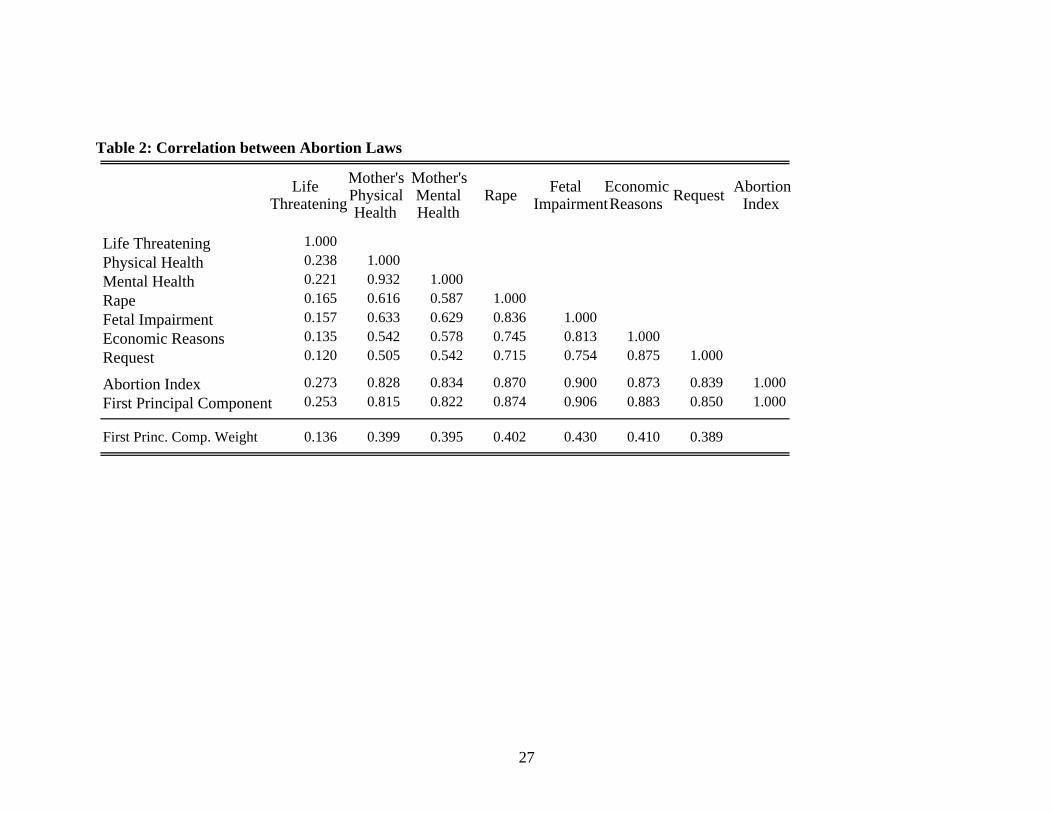
Table 2 shows the correlation matrix for the abortion variables. Apart from abortion when

the pregnancy threatens the life of the mother, which is almost universally allowed, the

other indicators are highly collinear. We find that each abortion variable has significant

explanatory power for fertility when used singularly, but additional abortion variables

add little to the fit of the first-stage regression. Accordingly, using more than one variable

may lead to a weak instrument problem, increasing the finite sample estimation bias.

Using multiple instruments would have the potential advantage of allowing an over-

identifying restrictions test of instrument validity; when we use multiple instruments we

indeed pass this test. However, this test relies on at least one instrument being valid and

lacks appeal in our context when the intuitive justification for each instrument is the

same, and it is likely that either all, or none, of our instruments are valid. These issues are

11

discussed in more detail in Murray (2006), and lead us to use only one instrument in our

analysis. Rather than using one of the raw abortion measures we use an abortion index

giving equal weight to each measure in an aggregate; this index has a slightly higher

predictive power for fertility than any single abortion measure.

As an alternative to using a simple additive index, one might consider using the

principal component of the seven abortion variables in the empirical analysis. As can be

seen in Table 2, the first principal component is virtually identical to the index we use in

our empirical specification. The correlation between the abortion index and the first

principal component is 0.997. The weight assigned to each of the abortion indicators in

the construction of the first principal component, shown on the final row of Table 2, is

almost identical for each measure (except for the “life threatening” category) making it

very similar to an additive index. For ease of interpretation, we use the abortion index

rather than the first principal component.

Our abortion index is correlated with fertility, but a key issue is that for abortion

legislation to be a valid instrument it must be uncorrelated with the error term in the

female labor market participation regression. It seems likely that the only way that

abortion laws affect labor market participation is through their effect on fertility. We

measure the effect through the total fertility rate. The total fertility rate is the number of

births a woman would have if she experienced the current age-specific fertility in the

population; this is a period rather than cohort measure. Thus it captures permanent shifts

in fertility as well as temporary shifts due to changes in the timing of births.

The instrument validity condition will hold if abortion legislation occurs

randomly, but this is highly unlikely. There are two ways instrument validity may break

down if abortion legislation is not random. The first is that abortion legislation is

endogenously responding to fertility desires, or to female labor force participation, so that

the direction of causality is the opposite to what we require of an instrument. The second

is that there are some unobserved variables, perhaps social or cultural norms, which

influence both abortion legislation and female labor force participation. We control for

the unobserved national social and cultural norms in our analysis using country fixed

12

effects, and country-specific time trends. This allows the average level and time trend of

the abortion index in a country to be endogenous. We identify the effect from abortion

legislation that deviates from the average level and time trend of the abortion legislation

index in that country. Although the level and time trend in abortion legislation may be

endogenous, we take the exact timing of abortion legislation, which generates deviations

from these long-term trends, to be random.

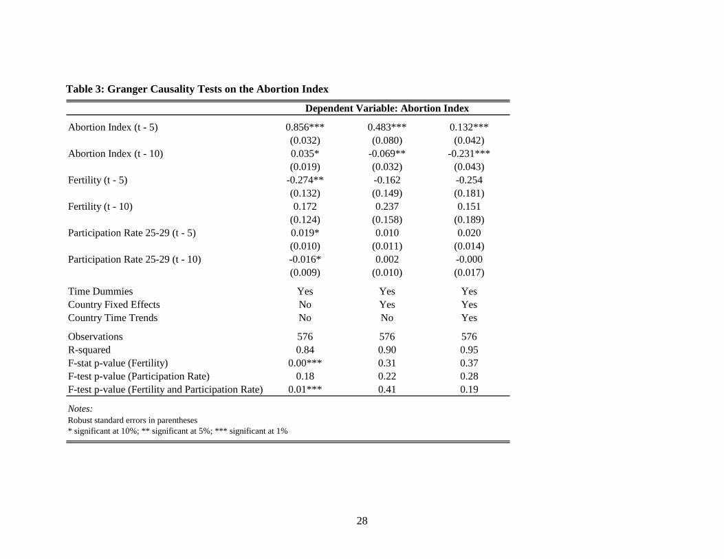
To examine the issue of reverse causality from fertility or female labor market

participation to abortion legislation we carry out Granger causality tests. The tests seek to

determine if lagged female labor force participation of a specific cohort and fertility are

predictive of abortion legislation. Table 3 reports the results of a regression of our

abortion legislation index on two lags of its own value, the female participation rate of

25–29 year olds (the age group whose participation we find is most sensitive to fertility)

and the total fertility rate. The first column includes worldwide time dummies, the second

column adds country fixed effects, while the third adds country-specific linear time

trends. The results in the first column suggest that a low fertility rate and high female

labor force participation rate are predictive of a higher value of the abortion legislation

index. However, this predictive power disappears in columns 2 and 3 of Table 4 when we

add country fixed effects (column 2) and country-specific time trends (column 3). These

results are consistent with the view that there are country-specific cultural factors that

drive fertility, female labor force participation, and abortion legislation. However, once

we control for these generic differences in levels and trends using country fixed effects

and time dummies, movements in the abortion law appear random.

[Table 3]

An alternative potential instrument in this context could be the measure of family

planning program effort compiled by Ross and Stover (2001). The family planning effort

score provides an aggregate of 30 scores on a range of variables that measure a

government’s commitment to family planning. We find that there is a positive correlation

between these effort scores and our abortion law index. We do not use the effort scores as

13

an instrument because of evidence that some of the scores measured may be highly

responsive to the demand for family planning (Kelly and Cutright 1983).

A final point about our instrument is that we treat the estimates as identifying a

single effect of fertility on female labor market participation. If there is heterogeneity in

the response across women, and abortion legislation only affects the fertility of a

subgroup of the population, it is the average labor market response to fertility within this

subgroup (the local average treatment effect) that we measure, not the population average

response.

5. Empirical Specification and Results

Equation 1.7 suggests that female labor force participation depends on the fertility

rate, the wage rate, and intra-family transfers. We include the fertility rate in our

empirical specification and proxy the wage rate of women by the ratio of capital per

working-age person, female life expectancy, and the female education level. The level of

intra-family transfers is captured using the male education level. In addition to these

variables, we add the percentage of the population living in urban areas. In agricultural

societies, the workplace is located around the family home, making it easier to

simultaneously care for children and work. In urban areas, by contrast, the workplace is

usually distinct from the home, making it more difficult to do both concurrently.

Moreover, urbanization can also have a negative effect on female labor supply during the

transition from agriculture to manufacturing. If working outside the home in manual

labor carries a social stigma for women, this may reduce their labor market opportunities

(Goldin 1995).

In our empirical work we estimate the following equation,

ijt i i jt i jt i jt i jt

f mi jt i jt it ij ij ijt

P Fert Cap Life Urban

Eduf Edum t

α β γ ϕ λ

φ φ δ δ τ ε

= + + + +

+ + + + + + (1.11)

14

where Pijt is the participation rate of females of age group i in country j at period t. Fert

is the total fertility rate, Cap is the capital stock per working-age person, Life is female

life expectancy, Urban is the percentage of the population living in urban areas, Edum is

the average years of schooling of men while Eduf is the average years of schooling of

women, δij and δit are country and year fixed effects, respectively, while ijτ denotes

country-specific time trends. Note that each of these fixed effects, time dummies, and

time trends can vary by age group, i. The country fixed effects, time dummies and

country-specific time trends allow for different labor market institutions and cultural

norms across countries and over time.

The inclusion of fixed effects and country-specific time trends makes the model

robust to unobserved heterogeneity, but comes at the cost of reducing the signal-to-noise

ratio. We therefore start our empirical analysis by estimating the model with fixed effect

but without country-specific time trends. The regression for the participation of each age

group is run separately. The results are reported for ten groups aged 15–64, although the

results for the first group, the age group 15–19, should be treated with caution because

labor market participation in this group is reduced by school attendance. The results for

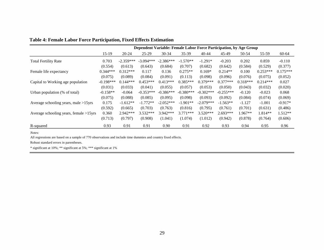
this specification, without instrumentation, are summarized in Table 4 below.

Table 4 shows that the marginal effect of fertility on female labor force

participation is negative and statistically significant for all age groups between 20 and 44.

Capital per working-age person, female life expectancy, and female education all appear

to have positive and relatively large effects on female labor participation (at least for ages

above 20). Male education reduces female labor market participation, which is consistent

with male earnings producing an income effect that lowers female work incentives. The

estimated coefficient on urbanization is negative; a 10 percentage point increase in

urbanization leads to a decrease in female labor force participation of between 2 and 5

percentage points. This effect implies high participation in rural economies, even when

female wages may be low.

[Table 4]

15

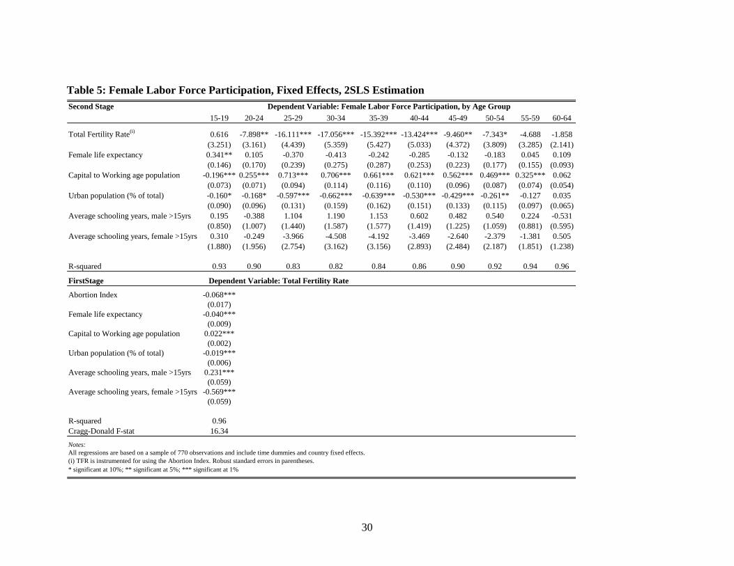
In Table 5, we use the abortion index as an instrument in a two-stage least squares

estimation as an alternative specification. The estimated fertility effects are very large:

according to the instrumental variable (IV) estimates, a unit decrease in the total fertility

rate leads to an increase of 5 to 17 percentage points in female labor force participation.

The point estimates from the IV estimation appear large in absolute magnitude

relative to the OLS estimates presented in Table 4. If higher female labor supply

depresses fertility, the OLS estimate should be larger, and not smaller than the IV

estimate. One possible explanation for this finding is that measurement error may

attenuate the OLS estimates but not the instrumental variable estimate. Another possible

explanation is that fertility and female labor supply are positively correlated due to some

unobserved variables (for example, the non-child-care time required for household tasks),

so that instrumentation reduces this omitted variable bias.

The bottom half of Table 5 reports the first-stage estimation of fertility. The

estimated effect of abortion laws on fertility is relatively small. The maximum increase in

the abortion index (from 0 to 7) leads to a predicted reduction in fertility of about 0.5

children. This effect appears reasonable, but is relatively small compared to the average

change in fertility rates observed in the sample period. The first stage F-statistic larger

than 16 suggests that abortion laws are highly predictive in the first-stage regression.

[Table 5]

In the OLS estimates in Table 4, female education is associated with higher

female labor market participation, while male education is associated with lower female

participation. In Table 5, when fertility is instrumented, these education effects on female

participation are not statistically significant. Note, however, that education has strong

effects on fertility in the first-stage regression reported in Table 5. Fertility falls as female

education levels rise, but rises with male education levels. Because the effect of female

education is larger, an equal rise in education for both sexes implies lower fertility. It

16

follows that, conditional on fertility, education may not be very significant in the

participation equation, but it still has a large impact on female labor market participation

through its effect on fertility. This is similar to the argument by Smith and Ward (1985)

that the effect of higher female wages on female labor supply works partly through

fertility reductions.

Although we control for country fixed effects and time dummies in the empirical

specifications presented in the previous section, one may still worry about country-

specific trends that are not picked up by time fixed effects. As individual societies

become westernized, more or less religious, or more open to trade, attitudes towards the

female role in society may change, affecting abortion legislation, fertility, and female

labor force participation. To control for such trends, we repeat the previous analysis

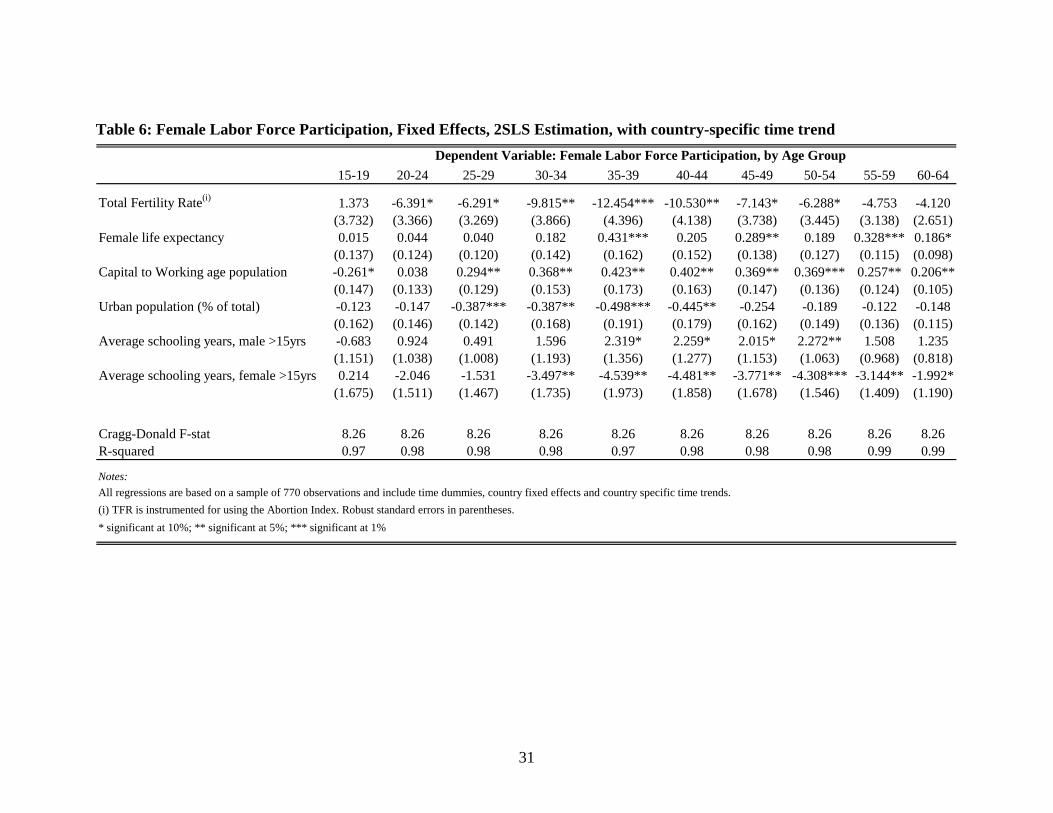
allowing for a country-specific time trend. The results, which are summarized in Table 6,

confirm our previous findings. The inclusion of a country-specific time trend slightly

lowers the point estimates on capital, urbanization and fertility, but does not change our

basic result: the average fertility response across the main age groups ranges from 6 to 12

percentage points.

[Table 6]

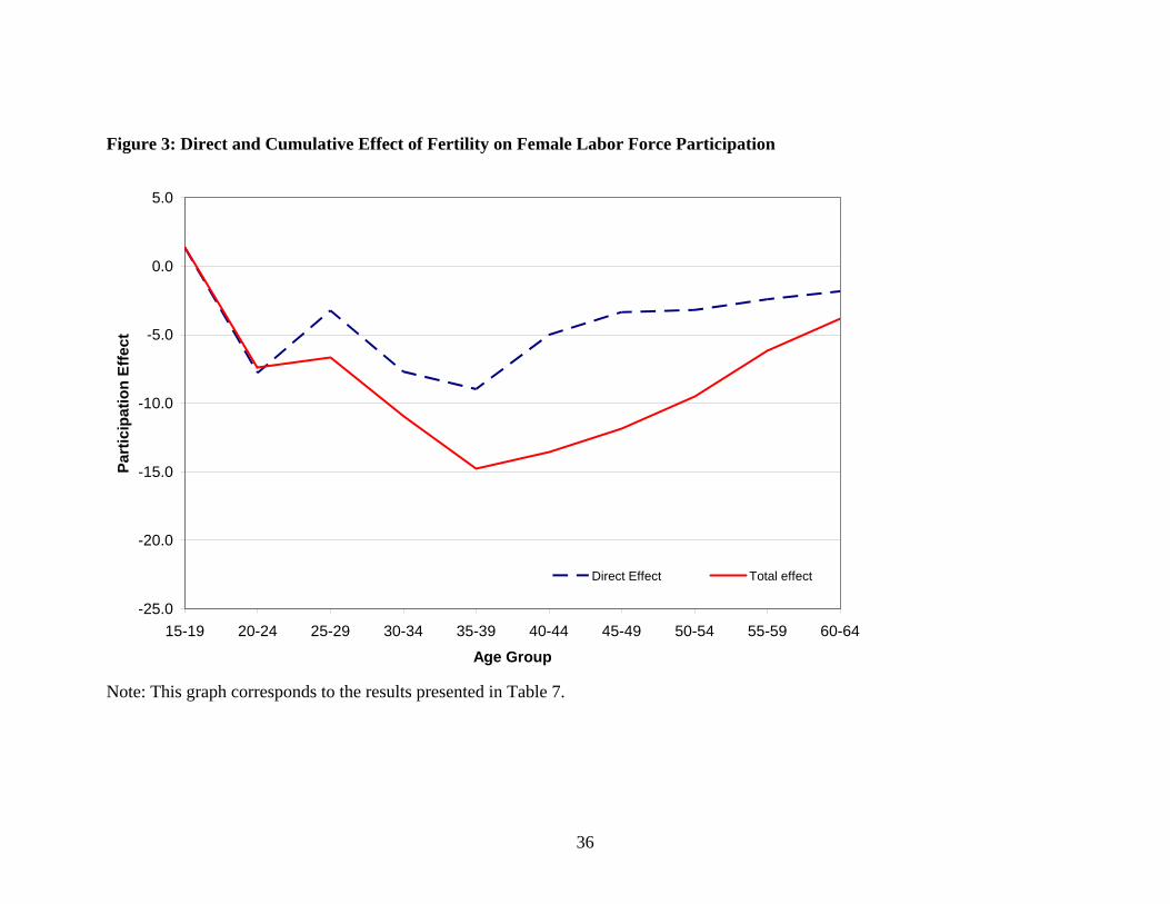
The effects of fertility on the labor participation of women appear to peak among

35–39 year olds, and are significant even for 50 year olds. We would expect fertility to

affect mainly younger women. However, exit from the labor market due to fertility may

have long-run effects if participation behavior is persistent. One reason for such

persistence might be returns to experience, which lower the wages of women who

temporarily exit the labor market relative to women who stay employed. To investigate

this, we include lagged cohort participation in the specifications shown in Table 7.

Because our lagged variable is the participation of a different age group – the age group

five years younger in the previous time period – rather than lagged participation of the

same age group, the problem of bias in a dynamic panel with short time dimension

(Nickell 1981) does not apply.

17

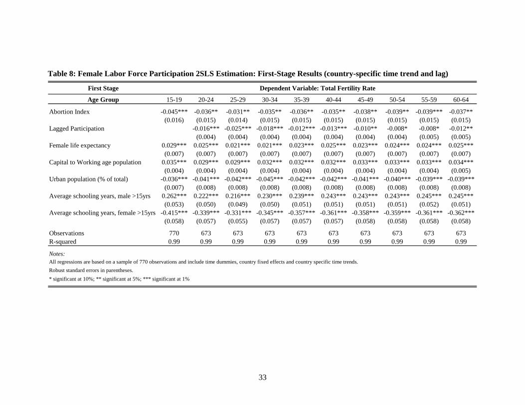
The results for the model with lagged participation included as an explanatory

variable are reported in Table 7. First-stage results for this specification are displayed in

Table 8. Note that the first stage for the 15–19 year olds (which does not include a lagged

participation term) is the same as the first stage for fertility when we do not include a lag

in the specification. This corresponds to the first stage of the static model reported in

Table 6. Female education is again highly significant in the first-stage regressions, and

education works indirectly through fertility rather than directly on labor market

participation. The abortion index is also highly significant in the first-stage regression.

Even when controlling for country fixed effects, time dummies, a country-specific

time trend, and a lagged cohort participation rate (Table 7), the highly significant

negative effect of fertility on female labor force participation persists. The marginal

effect of fertility is statistically significant for the age groups 20–24, 30–34 and 35–39,

but highly relevant for all age groups given the persistence of female labor force

participation. The significant coefficient on the lagged participation implies that the

fertility effect on participation at young ages may impact female labor force participation

throughout working life.

Although the dynamic framework reported in Tables 7 and 8 seems plausible, we

regard the results from the static model reported in Table 6 as our preferred estimates. In

the dynamic estimates, we need to assume the lagged cohort female labor force

participation to be exogenous. If the disturbances in the model are auto-correlated, this

assumption will not be valid. In principle, we can overcome this by instrumenting the

lagged participation rate. However, lagged abortion has little predictive power for lagged

participation, giving rise to the weak instrument problem. In a dynamic model with fixed

effects, country-specific time trends, and lagged participation, proper identification of a

2SLS model becomes difficult.

Overall, our static and dynamic models give very similar estimates of the long-run

effect of fertility on female labor market participation. Our estimates imply a reduction in

18

paid work of 8 percent of a woman’s potential working life, or 4 years of paid

employment, for each child born.

6. Simulations

To illustrate the magnitude of the growth effects associated with the demographic

transition, we provide simulation results. The Republic of Korea (South Korea) poses a

prime example for a developing country moving through the demographic transition, and

we calibrate our model to this economy. Total fertility rates in South Korea dropped from

5.6 children per woman in the early 1960s to 1.2 children in the period 2000–2005.

According to the United Nations, fertility rates in the South Korea are expected to reach

their low at 0.85 children in 2015 before gradually recovering to levels around 1.35 in the

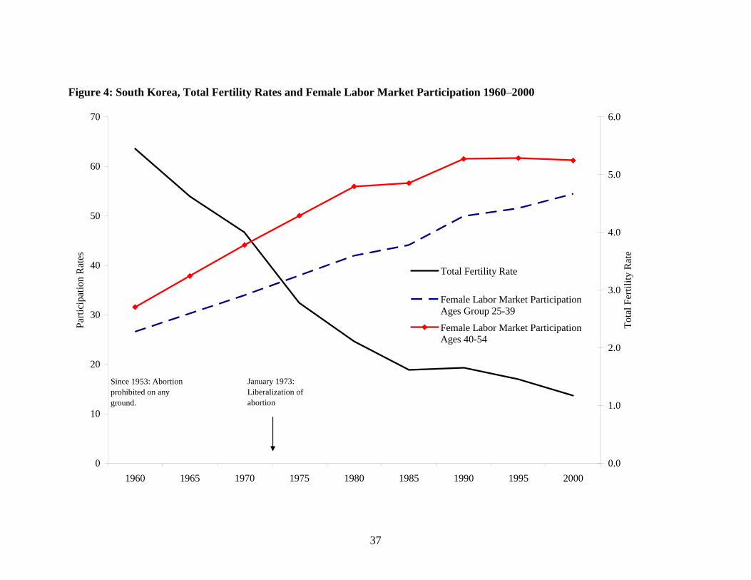
long run5 (World Population Prospects, 2004). As shown in Figure 4, the drop in fertility

over the last 40 years has been accompanied by a rapid increase in female labor force

participation rates: average participation in the age group 25–39 has risen from 26.6

percent in 1960 to 54.5 percent in 2000 (ILO Bureau of Statistics 2007).

[Figure 4]

The representative economy we simulate is based on a standard Cobb-Douglas

production function with constant returns to scale. Total output Y in each period t is given

by 1

t t tY AK Lα α−=

where A is a productivity measure, K is the stock of physical capital, and L denotes the

labor force. Technological progress and education are assumed to be constant and are

included in the parameter A. We are interested in how changes in the fertility rate affect

the labor force, the physical capital stock, and income per capita. The physical capital

stock Kt in each period t is determined by

5 The numbers cited reflect the United Nations' most conservative projections (low-fertility scenario). We use the low fertility scenario as it assumes a continuous decline in fertility for the next 15 years which is consistent with the trends in fertility observed over the past 20 years. Results using the other scenarios are very similar.

19

1 1(1 )t t tK sY Kδ− −= + − ,

where s is the aggregate savings rate and δ is the depreciation rate.

We initialize our simulations with the age structure in South Korea in 1960. The

evolution of population numbers and age structure after 1960 in the simulation differ

from the actual figures recorded in South Korea because we keep age-specific mortality

rates fixed at their 1960 levels.6 Our simulation therefore only captures the effect of

fertility decline on population, and not the impact of improved longevity. Modeling each

male and female birth cohort separately, the population sitP of sex s, age i, and time t is

given by

( )45

1, 1 1 016

1 1,s s s s fit i t i t s it it

iP P for i P f Pσ λ− − −

=

= − ≥ = ∑

where tf is the age-specific fertility rate7 at time t, and sλ is the fraction of sex s in

births. To determine the size of the population we take the age- and sex-specific mortality

rates siσ to be fixed at the 1960 levels.8 The sex ratio at birth is set at 51 percent male

and 49 percent female, which corresponds to the makeup of the current adult population

in South Korea.9

The labor force Lt used in production in each period t is given by 100

0 ,

,s st it it

i s m f

L P ρ= =

=∑ ∑

where sitρ captures the age- and gender-specific labor participation rates at time t.

We assume capital and labor shares in income to be one third and two thirds

respectively (so that 1/ 3α = ). Our other baseline assumptions are a savings rate s of 24 6 We also perform alternative specifications with actual and predicted survival tables for the period 1960 to 2050. The results look very similar to the ones presented in this section. 7 We assume that fertility is distributed uniformly over the fertile years as the exact age of birth is unknown in the aggregate data. 8 Note that (1-σi) is the survival probability between age i and age i+1. 9 In recent years, the percentage of female newborns has fallen to 47%; we take the average of the last 30 years as our baseline assumption.

20

percent and an annual capital stock depreciation rate of 8 percent. This gives a steady-

state capital output ratio of three. Rather than estimating the capital stock for South Korea

in 1960, we assume that the economy starts in steady state with a steady level of GDP per

capita. This is the steady state that would have emerged if fertility rates, participation

rates, and mortality schedules had remained at the 1960 levels. Because we consider only

relative output levels, we set the level of total factor productivity A to one without loss

of generality.

The only exogenous variable that we change during the simulation is the fertility

rate, for which we use the actual and forecast rates as published by the United Nations

(2004). Although we assume that male participation rates remain constant at 1960 levels,

we allow for female labor force participation to respond to the lower fertility in line with

the estimates reported in Table 6.

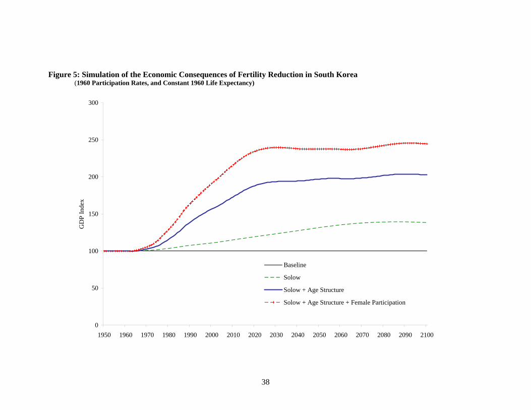
We report our simulation results in Figure 5. The baseline is the steady-state

income per capita level at constant 1960 fertility rates. We then consider the effect of the

actual and predicted future decline in fertility rates relative to this baseline. We first

estimate the Solow effect of lower population growth on the capital-labor ratio.

Assuming that the ratio of workers to population is constant as in the standard Solow

model, lower fertility rates imply lower population growth, a higher capital-labor ratio

and higher output per capita. According to our model, income per capita rises by 36

percent if we take only this Solow effect into account.

[Figure 5]

However, falling fertility also translates to changes in the population age

structure. Keeping age- and sex-specific participation rates constant at the 1960 levels,

the “Solow plus age structure” effect in Figure 5 combines the Solow capital-labor effect

with the high labor supply per capita due to a falling youth dependency ratio. Assuming

that male and female (age-specific) participation rates do not change, the shift in age

structure implies that the percentage of population working increases from 31 to 46

21

percent in the long run. This leads to an additional 47 percent in steady-state output per

capita over and above the Solow effect.10 It should be noted that the transition is not

monotonic. The rapid decline in fertility generates a “baby boom cohort,” whose

members produce high output during their working age, but also a high old-age

dependency rate once they retire. This cohort effect is very mild in our simulation. Even

when we include the effect of longer life spans on age structure, the decrease in the youth

dependency generated by the fertility decline dominates the increase in old-age

dependency, such that the overall dependency rate declines. This effect is even stronger

when old-age participation rates are high as is the case in South Korea.

The effects on income per capita are even bigger once we allow for female labor

market participation to adjust to lower fertility. Using our point estimates from Table 6 to

simulate the female labor supply responses, we find that the female labor supply response

leads to an additional increase of steady-state income per capita of 21 percent relative to

the scenario with the Solow and age structure effect. Combining all effects implies an

increase in steady-state per capita income of 141 percent relative to the base line.11 The

results suggest that reductions in fertility increased the growth rate of per capita income

in South Korea by 1.9 percent per year between 1960 and 1990. Between 1990 and 2020

the effect is smaller, increasing the growth rate by 1.2 percent per year. Our simulation

suggests that economic growth from this source will end around 2020, but that the high

level of income attained due to low fertility will persist.

Our simulation examines only the effects of fertility decline. In fact, since 1960

there have been large reductions in mortality rates in South Korea, particularly at older

ages, while old-age labor market participation rates have declined. Including these effects

in the simulation reduces the gain in income per capita somewhat and produces a more

pronounced downturn in income per capita after 2020 due to population aging and earlier

retirement, though the long run steady-state income level stays well above its 1960 level.

10 The effects do not add up linearly because the capital-labor ratio “Solow” effect is somewhat reduced by higher labor force participation. 11 The individual effects multiply each other; 36 percent Solow effect is multiplied by 47 percent from age structure and 21 percent from the female labor supply response: (1.36 1.47 1.21 2.41)× × = .

22

7. Discussion and Conclusions

The concept of the "demographic dividend" (Bloom, Canning et al. 2001; Bloom,

Canning et al. 2003) elucidates the economic benefits that a country can gain if it

experiences a decline in fertility. The decline in fertility reduces population growth, and

increases the capital-labor ratio. At the same time, the shift in fertility increases the ratio

of working-age to total population; compounding this is the positive behavioral response

of female labor force participation, which further increases labor supply per capita. Using

a simulation model, our parameter estimates suggest that the effects of fertility reduction

on income levels can be large – more than doubling the steady-state level of output per

capita.

In this paper, we have only considered the effect of fertility on female labor

supply. The model presented here does not account for the possible effect on education of

a decline in fertility. Increased female labor supply may raise the economic returns to

women’s schooling, providing positive incentives for women to invest in education. The

effect of fertility on saving is another important aspect not taken into account. To the

extent that children provide old-age support to their parents, a decline in fertility may

increase financial savings for old age and retirement. The decline in fertility may also

have beneficial effects on long-run economic growth by allowing greater investment in

children’s health and education. These mechanisms suggest that the overall effect of a

fertility decline on economic growth may be even larger than we report.

23

8. References

Angrist, J. and W. Evans (1998). "Children and Their Parents' Labor Supply: Evidence from Exogenous Variation in Family Size." American Economic Review 88(3): 450-477. Angrist, J. D. and W. N. Evans (1996). "Schooling and Labor Market Consequences of the 1970 State Abortion Reforms." NBER Working Paper W5406. Bailey, M. J. (2006). "More power to the pill: The impact of contraceptive freedom on women's lifecycle labor supply." Quarterly Journal of Economics 121 (1): 289-320. Barro, R. J. and J.-W. Lee (2000). "International Data on Educational Attainment: Updates and Implications." CID Working Paper 42. Bloom, D. E., D. Canning, et al. (2000). "Population Dynamics and Economic Growth in Asia." Journal of Population Economics 26(supp.): 257-90. Bloom, D. E., D. Canning, et al. (2007). "Demographic Change, Social Security Systems, and Savings." Journal of Monetary Economics 54(1): 92-114. Bloom, D. E., D. Canning, et al. (2001). "Economic Growth and the Demographic Transition." NBER Working Paper(8685). Bloom, D. E., D. Canning, et al. (2003). "The Demographic Dividend: A New Perspective on the Economic Consequences of Population Change." RAND Monograph Report. Bloom, D. E. and R. B. Freeman (1987). "Population Growth, Labor Supply, and Employment in Developing Countries." Population growth and economic development: Issues and evidence. Bloom, D. E. and J. G. Williamson (1998). "Demographic transitions and economic miracles in emerging Asia." World Bank Economic Review 12(3): 419-455. Bongaarts, J. (1984). "Implications for future fertility trends for contraceptive practice." Population and Development Review 10(2): 341-352. Brander, J. A. and S. Dowrick (1994). "The Role of Fertility and Population in Economic Growth." Journal of Population Economics 7(1): 1-25. Browning, M. (1992). "Children and Household Economic Behavior." Journal of Economic Literature 30(3): 1434-1475. Engelhardt, H. and A. Prskawetz (2004). "On the changing correlation between fertility and female employment over space and time." European Journal of Population 20: 35-62.

24

Goldin, C. (1995). The U-Shaped Female Labor Force Function in Economic Development and Economic History. Investment in Women's Human Capital and Economic Development. T. P. Schultz. Chicago, IL, University of Chicago Press: 61-90. Henshaw, S. K., S. Singh, et al. (1999). "The Incidence of Abortion Worldwide." International Family Planning Perspectives 25(Supplement): S30-S38. Heston, A., R. Summers, et al. (2006). "Penn World Table Version 6.2." Center for International Comparisons of Production, Income and Prices at the University of Pennsylvania. ILO (1997). Economically Active Population, 1950-2010. Geneva. ILO Bureau of Statistics (2007). ILO Database on Labour Statistics, International Labour Organization. Kelley, A. C. and R. M. Schmidt (1995). "Aggregate Population and Economic Growth Correlations: The Role of the Components of Demographic Change." Demography 32(4): 543-555. Kelly, W. R. and P. Cutright (1983). "Determinants of national family planning effort." Population Research and Policy Review 2(2): 111-130. Klerman, J. A. (1999). "U.S. Abortion Policy and Fertility " The American Economic Review 89(2): 261-264. Levine, P. B., D. Staiger, et al. (1999). "Roe v Wade and American fertility." American Journal of Public Health 89(2): 199-203. Mammen, K. and C. Paxson (2000). "Women's Work and Economic Development." The Journal of Economic Perspectives 14(4): 141-164. Murray, M. P. (2006). Econometrics: A Modern Introduction. Boston, Addison-Wesley. Nickell, S. (1981). "Biases in dynamic models with fixed effects." Econometrica 49(6): 1417-1426. Rosenzweig, M. R. and K. I. Wolpin (1980). "Testing the Quantity-Quality Fertility Model: The Use of Twins as a Natural Experiment." Econometrica 48(1): 227-240. Ross, J. and J. Stover (2001). "The family planning program effort index: 1999 cycle." International Family Planning Perspectives 27(3): 119-129. Simon, J. L. (1989). "On Aggregate Empirical Studies Relating Population Variables to Economic Development." Population and Development Review 15(2): 323-332.

25

Smith, J. P. and M. P. Ward (1985). "Time-Series Growth in the Female Labor Force." Journal of Labor Economics 3(1): 59-90. United Nations (2004). World Population Prospects CD-ROM. United Nations Population Division. (2002). "Abortion Policies: A Global Review." 2007, from http://www.un.org/esa/population/publications/abortion/index.htm. World Bank (2006). "World Bank Development Indicators CD-ROM."

26

Table 1: Summary Statistics

Variable Name Mean Std. Dev. Min Max

Abortion: Pregnancy Life Threatening 0.95 0.21 0 1Abortion: Pregnancy Threatening Physical Health 0.56 0.50 0 1Abortion: Pregnancy Treatening Mental Health 0.52 0.50 0 1Abortion: Rape 0.37 0.48 0 1Abortion: Fetal Impairment 0.32 0.47 0 1Abortion: Economic Reasons 0.22 0.42 0 1Abortion: Request 0.17 0.37 0 1Abortion Index 3.11 2.29 0 7Total Fertility Rate 4.35 2.04 1.18 8.50Average years of schooling, male, age >15 5.4 2.8 0.3 12.2Average years of schooling, female, age >15 4.5 3.0 0.0 12.0Capital per Working Age Person 23.2 27.4 0.3 138.2Female Life Expectancy at birth 64.1 12.6 33.4 84.6Urban population (% of total) 48.1 24.7 3.2 100Real GDP per capita (Real 2004 $, PPP) 7,340 7,531 171 64,640Female Participation Age 15-19 39.0 19.0 3.6 89.0Female Participation Age 20-24 55.8 18.4 12.2 100.0Female Participation Age 24-29 55.7 19.8 10.9 100.0Female Participation Age 30-34 55.7 21.4 12.5 100.0Female Participation Age 35-39 56.5 22.4 11.9 100.0Female Participation Age 40-44 56.5 22.7 11.7 100.0Female Participation Age 45-49 54.7 23.0 8.7 100.0Female Participation Age 50-54 50.2 22.8 5.4 98.0Female Participation Age 55-59 43.3 22.7 3.1 94.2Female Participation Age 60-64 33.1 21.8 1.2 88.9Notes: Based on the sample of 770 observations

27

Table 2: Correlation between Abortion Laws

Life Threatening

Mother's Physical Health

Mother's Mental Health

Rape Fetal Impairment

Economic Reasons Request Abortion

Index

Life Threatening 1.000Physical Health 0.238 1.000Mental Health 0.221 0.932 1.000Rape 0.165 0.616 0.587 1.000Fetal Impairment 0.157 0.633 0.629 0.836 1.000Economic Reasons 0.135 0.542 0.578 0.745 0.813 1.000Request 0.120 0.505 0.542 0.715 0.754 0.875 1.000

Abortion Index 0.273 0.828 0.834 0.870 0.900 0.873 0.839 1.000First Principal Component 0.253 0.815 0.822 0.874 0.906 0.883 0.850 1.000

First Princ. Comp. Weight 0.136 0.399 0.395 0.402 0.430 0.410 0.389

28

Table 3: Granger Causality Tests on the Abortion Index

Abortion Index (t - 5) 0.856*** 0.483*** 0.132***(0.032) (0.080) (0.042)

Abortion Index (t - 10) 0.035* -0.069** -0.231***(0.019) (0.032) (0.043)

Fertility (t - 5) -0.274** -0.162 -0.254(0.132) (0.149) (0.181)

Fertility (t - 10) 0.172 0.237 0.151(0.124) (0.158) (0.189)

Participation Rate 25-29 (t - 5) 0.019* 0.010 0.020(0.010) (0.011) (0.014)

Participation Rate 25-29 (t - 10) -0.016* 0.002 -0.000(0.009) (0.010) (0.017)

Time Dummies Yes Yes YesCountry Fixed Effects No Yes YesCountry Time Trends No No Yes

Observations 576 576 576R-squared 0.84 0.90 0.95F-stat p-value (Fertility) 0.00*** 0.31 0.37F-test p-value (Participation Rate) 0.18 0.22 0.28F-test p-value (Fertility and Participation Rate) 0.01*** 0.41 0.19

Notes:

Dependent Variable: Abortion Index

Robust standard errors in parentheses* significant at 10%; ** significant at 5%; *** significant at 1%

29

Table 4: Female Labor Force Participation, Fixed Effects Estimation

15-19 20-24 25-29 30-34 35-39 40-44 45-49 50-54 55-59 60-64

Total Fertility Rate 0.703 -2.359*** -3.094*** -2.386*** -1.570** -1.291* -0.203 0.202 0.859 -0.110(0.554) (0.613) (0.643) (0.684) (0.707) (0.682) (0.642) (0.584) (0.529) (0.377)

Female life expectancy 0.344*** 0.312*** 0.117 0.136 0.275** 0.169* 0.214** 0.100 0.253*** 0.175***(0.075) (0.089) (0.084) (0.091) (0.113) (0.098) (0.096) (0.076) (0.075) (0.052)

Capital to Working age population -0.198*** 0.144*** 0.453*** 0.413*** 0.385*** 0.379*** 0.377*** 0.318*** 0.214*** 0.027(0.031) (0.033) (0.041) (0.055) (0.057) (0.053) (0.050) (0.043) (0.032) (0.020)

Urban population (% of total) -0.158** -0.064 -0.353*** -0.386*** -0.380*** -0.302*** -0.255*** -0.120 -0.023 0.068(0.075) (0.088) (0.085) (0.095) (0.098) (0.093) (0.092) (0.084) (0.074) (0.069)

Average schooling years, male >15yrs 0.175 -1.612** -1.772** -2.052*** -1.901** -2.079*** -1.563** -1.127 -1.001 -0.917*(0.592) (0.665) (0.703) (0.763) (0.816) (0.795) (0.761) (0.701) (0.631) (0.486)

Average schooling years, female >15yrs 0.360 2.942*** 3.532*** 3.942*** 3.771*** 3.520*** 2.693*** 1.967** 1.814** 1.512**(0.713) (0.797) (0.908) (1.041) (1.074) (1.012) (0.942) (0.878) (0.764) (0.606)

R-squared 0.93 0.91 0.91 0.90 0.91 0.92 0.93 0.94 0.95 0.96Notes:

* significant at 10%; ** significant at 5%; *** significant at 1%

All regressions are based on a sample of 770 observations and include time dummies and country fixed effects. Robust standard errors in parentheses.

Dependent Variable: Female Labor Force Participation, by Age Group

30

Table 5: Female Labor Force Participation, Fixed Effects, 2SLS Estimation Second Stage

15-19 20-24 25-29 30-34 35-39 40-44 45-49 50-54 55-59 60-64

Total Fertility Rate(i) 0.616 -7.898** -16.111*** -17.056*** -15.392*** -13.424*** -9.460** -7.343* -4.688 -1.858(3.251) (3.161) (4.439) (5.359) (5.427) (5.033) (4.372) (3.809) (3.285) (2.141)

Female life expectancy 0.341** 0.105 -0.370 -0.413 -0.242 -0.285 -0.132 -0.183 0.045 0.109(0.146) (0.170) (0.239) (0.275) (0.287) (0.253) (0.223) (0.177) (0.155) (0.093)

Capital to Working age population -0.196*** 0.255*** 0.713*** 0.706*** 0.661*** 0.621*** 0.562*** 0.469*** 0.325*** 0.062(0.073) (0.071) (0.094) (0.114) (0.116) (0.110) (0.096) (0.087) (0.074) (0.054)

Urban population (% of total) -0.160* -0.168* -0.597*** -0.662*** -0.639*** -0.530*** -0.429*** -0.261** -0.127 0.035(0.090) (0.096) (0.131) (0.159) (0.162) (0.151) (0.133) (0.115) (0.097) (0.065)

Average schooling years, male >15yrs 0.195 -0.388 1.104 1.190 1.153 0.602 0.482 0.540 0.224 -0.531(0.850) (1.007) (1.440) (1.587) (1.577) (1.419) (1.225) (1.059) (0.881) (0.595)

Average schooling years, female >15yrs 0.310 -0.249 -3.966 -4.508 -4.192 -3.469 -2.640 -2.379 -1.381 0.505(1.880) (1.956) (2.754) (3.162) (3.156) (2.893) (2.484) (2.187) (1.851) (1.238)

R-squared 0.93 0.90 0.83 0.82 0.84 0.86 0.90 0.92 0.94 0.96

FirstStage

Abortion Index -0.068***(0.017)

Female life expectancy -0.040***(0.009)

Capital to Working age population 0.022***(0.002)

Urban population (% of total) -0.019***(0.006)

Average schooling years, male >15yrs 0.231***(0.059)

Average schooling years, female >15yrs -0.569***(0.059)

R-squared 0.96Cragg-Donald F-stat 16.34

Notes:

* significant at 10%; ** significant at 5%; *** significant at 1%

All regressions are based on a sample of 770 observations and include time dummies and country fixed effects. (i) TFR is instrumented for using the Abortion Index. Robust standard errors in parentheses.

Dependent Variable: Female Labor Force Participation, by Age Group

Dependent Variable: Total Fertility Rate

31

Table 6: Female Labor Force Participation, Fixed Effects, 2SLS Estimation, with country-specific time trend

15-19 20-24 25-29 30-34 35-39 40-44 45-49 50-54 55-59 60-64

Total Fertility Rate(i) 1.373 -6.391* -6.291* -9.815** -12.454*** -10.530** -7.143* -6.288* -4.753 -4.120(3.732) (3.366) (3.269) (3.866) (4.396) (4.138) (3.738) (3.445) (3.138) (2.651)

Female life expectancy 0.015 0.044 0.040 0.182 0.431*** 0.205 0.289** 0.189 0.328*** 0.186*(0.137) (0.124) (0.120) (0.142) (0.162) (0.152) (0.138) (0.127) (0.115) (0.098)

Capital to Working age population -0.261* 0.038 0.294** 0.368** 0.423** 0.402** 0.369** 0.369*** 0.257** 0.206**(0.147) (0.133) (0.129) (0.153) (0.173) (0.163) (0.147) (0.136) (0.124) (0.105)

Urban population (% of total) -0.123 -0.147 -0.387*** -0.387** -0.498*** -0.445** -0.254 -0.189 -0.122 -0.148(0.162) (0.146) (0.142) (0.168) (0.191) (0.179) (0.162) (0.149) (0.136) (0.115)

Average schooling years, male >15yrs -0.683 0.924 0.491 1.596 2.319* 2.259* 2.015* 2.272** 1.508 1.235(1.151) (1.038) (1.008) (1.193) (1.356) (1.277) (1.153) (1.063) (0.968) (0.818)

Average schooling years, female >15yrs 0.214 -2.046 -1.531 -3.497** -4.539** -4.481** -3.771** -4.308*** -3.144** -1.992*(1.675) (1.511) (1.467) (1.735) (1.973) (1.858) (1.678) (1.546) (1.409) (1.190)

Cragg-Donald F-stat 8.26 8.26 8.26 8.26 8.26 8.26 8.26 8.26 8.26 8.26R-squared 0.97 0.98 0.98 0.98 0.97 0.98 0.98 0.98 0.99 0.99

Notes:

* significant at 10%; ** significant at 5%; *** significant at 1%(i) TFR is instrumented for using the Abortion Index. Robust standard errors in parentheses.All regressions are based on a sample of 770 observations and include time dummies, country fixed effects and country specific time trends.

Dependent Variable: Female Labor Force Participation, by Age Group

32

Table 7: Female Labor Force Participation Fixed Effects, 2SLS Estimation with a Country Specific Trend and Lagged Female Labor Force Participation Rate

15-19 20-24 25-29 30-34 35-39 40-44 45-49 50-54 55-59 60-64

Total Fertility Rate(i) 1.373 -7.779* -3.227 -7.686* -8.957** -5.008 -3.348 -3.185 -2.416 -1.826(3.732) (4.133) (4.228) (3.975) (4.057) (3.533) (3.167) (3.094) (3.154) (2.759)

Lagged Participation 0.262*** 0.460*** 0.497*** 0.527*** 0.581*** 0.627*** 0.529*** 0.396*** 0.325***(0.077) (0.113) (0.083) (0.065) (0.058) (0.046) (0.044) (0.046) (0.050)

Female life expectancy 0.015 0.029 -0.014 0.165 0.355*** 0.016 0.230** 0.089 0.267*** 0.097(0.137) (0.129) (0.111) (0.110) (0.118) (0.108) (0.095) (0.097) (0.099) (0.087)

Capital to Working age population -0.261* 0.104 0.182 0.201 0.210 0.154 0.138 0.178 0.097 0.077(0.147) (0.135) (0.133) (0.141) (0.144) (0.123) (0.115) (0.114) (0.117) (0.103)

Urban population (% of total) -0.123 -0.216 -0.316 -0.242 -0.411** -0.236 -0.099 -0.134 -0.140 -0.184(0.162) (0.195) (0.196) (0.202) (0.193) (0.168) (0.151) (0.145) (0.146) (0.125)

Average schooling years, male >15yrs -0.683 1.223 -0.183 0.728 0.702 -0.004 0.050 0.454 0.212 0.376(1.151) (1.062) (1.023) (1.043) (1.103) (0.971) (0.884) (0.870) (0.894) (0.772)

Average schooling years, female >15yrs 0.214 -2.049 -0.007 -1.612 -1.455 -0.526 -0.491 -1.330 -1.019 -0.576(1.675) (1.525) (1.495) (1.483) (1.564) (1.373) (1.237) (1.216) (1.248) (1.088)

Cragg-Donald F-stat 8.26 5.96 4.53 5.71 5.76 5.53 6.40 6.62 6.75 6.12R-squared 0.97 0.98 0.99 0.99 0.99 0.99 0.99 0.99 0.99 0.99Number of Observations 770 673 673 673 673 673 673 673 673 673

Notes:

* significant at 10%; ** significant at 5%; *** significant at 1%

All regressions are based on a sample of 770 observations and include time dummies, country fixed effects and country specific time trends. (i) TFR is instrumented for using the Abortion Index. Robust standard errors in parentheses.

Dependent Variable: Female Labor Force Participation, by Age Group

33

Table 8: Female Labor Force Participation 2SLS Estimation: First-Stage Results (country-specific time trend and lag)

First Stage

Age Group 15-19 20-24 25-29 30-34 35-39 40-44 45-49 50-54 55-59 60-64

Abortion Index -0.045*** -0.036** -0.031** -0.035** -0.036** -0.035** -0.038** -0.039** -0.039*** -0.037**(0.016) (0.015) (0.014) (0.015) (0.015) (0.015) (0.015) (0.015) (0.015) (0.015)

Lagged Participation -0.016*** -0.025*** -0.018*** -0.012*** -0.013*** -0.010** -0.008* -0.008* -0.012**(0.004) (0.004) (0.004) (0.004) (0.004) (0.004) (0.004) (0.005) (0.005)

Female life expectancy 0.029*** 0.025*** 0.021*** 0.021*** 0.023*** 0.025*** 0.023*** 0.024*** 0.024*** 0.025***(0.007) (0.007) (0.007) (0.007) (0.007) (0.007) (0.007) (0.007) (0.007) (0.007)

Capital to Working age population 0.035*** 0.029*** 0.029*** 0.032*** 0.032*** 0.032*** 0.033*** 0.033*** 0.033*** 0.034***(0.004) (0.004) (0.004) (0.004) (0.004) (0.004) (0.004) (0.004) (0.004) (0.005)

Urban population (% of total) -0.036*** -0.041*** -0.042*** -0.045*** -0.042*** -0.042*** -0.041*** -0.040*** -0.039*** -0.039***(0.007) (0.008) (0.008) (0.008) (0.008) (0.008) (0.008) (0.008) (0.008) (0.008)

Average schooling years, male >15yrs 0.262*** 0.222*** 0.216*** 0.230*** 0.239*** 0.243*** 0.243*** 0.243*** 0.245*** 0.245***(0.053) (0.050) (0.049) (0.050) (0.051) (0.051) (0.051) (0.051) (0.052) (0.051)

Average schooling years, female >15yrs -0.415*** -0.339*** -0.331*** -0.345*** -0.357*** -0.361*** -0.358*** -0.359*** -0.361*** -0.362***(0.058) (0.057) (0.055) (0.057) (0.057) (0.057) (0.058) (0.058) (0.058) (0.058)

Observations 770 673 673 673 673 673 673 673 673 673R-squared 0.99 0.99 0.99 0.99 0.99 0.99 0.99 0.99 0.99 0.99

Notes:

* significant at 10%; ** significant at 5%; *** significant at 1%

All regressions are based on a sample of 770 observations and include time dummies, country fixed effects and country specific time trends. Robust standard errors in parentheses.

Dependent Variable: Total Fertility Rate

34

Figure 1: Income per Capita and Female Labor Force Participation 2000

TanzaniaMozambique

SudanEgypt

Thailand

Iceland

US

0

10

20

30

40

50

60

70

80

90

100

6 6.5 7 7.5 8 8.5 9 9.5 10 10.5 11

Log (Real GDP per Capita 2000)

Fem

ale

Labo

r For

ce P

artic

ipat

ion

Rat

e 20

00

35

Figure 2: Income per Capita 1980 and Change in Female Labor Force Participation 1980–2000

Ireland

Guinea-Bissau

Bangladesh

Turkey

Hungary

Peru

Ecuador

Sweden

Switzerland

Kuwait

-30

-20

-10

0

10

20

30

40

6 7 8 9 10 11

Log (Real GDP per Capita 1980)

Cha

nge

in F

emal

e La

bor F

orce

Par

ticip

atio

n 19

80-2

000

36

Figure 3: Direct and Cumulative Effect of Fertility on Female Labor Force Participation

-25.0

-20.0

-15.0

-10.0

-5.0

0.0

5.0

15-19 20-24 25-29 30-34 35-39 40-44 45-49 50-54 55-59 60-64

Age Group

Part

icip

atio

n Ef

fect

Direct Effect Total effect

Note: This graph corresponds to the results presented in Table 7.

37

Figure 4: South Korea, Total Fertility Rates and Female Labor Market Participation 1960–2000

0

10

20

30

40

50

60

70

1960 1965 1970 1975 1980 1985 1990 1995 2000

Parti

cipa

tion

Rat

es

0.0

1.0

2.0

3.0

4.0

5.0

6.0

Tota

l Fer

tility

Rat

e

Total Fertility Rate

Female Labor Market ParticipationAges Group 25-39

Female Labor Market ParticipationAges 40-54

January 1973: Liberalization of abortion

Since 1953: Abortion prohibited on any ground.

38

Figure 5: Simulation of the Economic Consequences of Fertility Reduction in South Korea

(1960 Participation Rates, and Constant 1960 Life Expectancy)

0

50

100

150

200

250

300

1950 1960 1970 1980 1990 2000 2010 2020 2030 2040 2050 2060 2070 2080 2090 2100

GD

P In

dex

Baseline

Solow

Solow + Age Structure

Solow + Age Structure + Female Participation

39

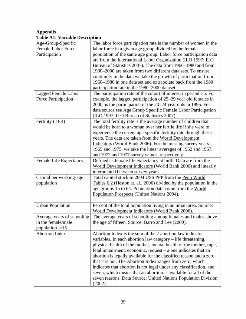
Appendix Table A1: Variable Description Age-Group-Specific Female Labor Force Participation

The labor force participation rate is the number of women in the labor force in a given age group divided by the female population of the same age group. Labor force participation data are from the International Labor Organization (ILO 1997; ILO Bureau of Statistics 2007). The data from 1960–1980 and from 1980–2000 are taken from two different data sets. To ensure continuity in the data we take the growth of participation from 1960–1980 in one data set and extrapolate back from the 1980 participation rate in the 1980–2000 dataset.

Lagged Female Labor Force Participation

The participation rate of the cohort of interest in period t-5. For example, the lagged participation of 25–29 year old females in 2000, is the participation of the 20–24 year olds in 1995. For data source see Age Group Specific Female Labor Participation (ILO 1997; ILO Bureau of Statistics 2007).

Fertility (TFR) The total fertility rate is the average number of children that would be born to a woman over her fertile life if she were to experience the current age-specific fertility rate through these years. The data are taken from the World Development Indicators (World Bank 2006). For the missing survey years 1965 and 1975, we take the linear averages of 1962 and 1967, and 1972 and 1977 survey values, respectively.

Female Life Expectancy Defined as female life expectancy at birth. Data are from the World Development Indicators (World Bank 2006) and linearly interpolated between survey years.

Capital per working-age population

Total capital stock in 2004 US$ PPP from the Penn World Tables 6.2 (Heston et. al., 2006) divided by the population in the age groups 15 to 64. Population data come from the World Population Prospects (United Nations 2004).

Urban Population Percent of the total population living in an urban area. Source: World Development Indicators (World Bank 2006).

Average years of schooling in the female/male population >15

The average years of schooling among females and males above the age of fifteen. Source: Barro and Lee (2000).

Abortion Index Abortion Index is the sum of the 7 abortion law indicator variables. In each abortion law category – life threatening, physical health of the mother, mental health of the mother, rape, fetal impairment, economic, request – a one indicates that an abortion is legally available for the classified reason and a zero that it is not. The Abortion Index ranges from zero, which indicates that abortion is not legal under any classification, and seven, which means that an abortion is available for all of the seven reasons. Data Source: United Nations Population Division (2002).

40

Table A2: Country List

1 Afghanistan 34 Guinea-Bissau 67 Panama 2 Algeria 35 Haiti 68 Papua New Guinea 3 Argentina 36 Honduras 69 Peru 4 Australia 37 Hungary 70 Philippines 5 Austria 38 Iceland 71 Poland 6 Bahrain 39 India 72 Portugal 7 Bangladesh 40 Indonesia 73 Rwanda 8 Barbados 41 Iran, Islamic Rep. 74 Senegal 9 Belgium 42 Iraq 75 Sierra Leone

10 Benin 43 Ireland 76 Singapore 11 Botswana 44 Israel 77 South Africa 12 Brazil 45 Italy 78 Spain 13 Cameroon 46 Jamaica 79 Sri Lanka 14 Canada 47 Japan 80 Sudan 15 Central African Republic 48 Jordan 81 Swaziland 16 Chile 49 Kenya 82 Sweden 17 China 50 Korea, Rep. 83 Switzerland 18 Colombia 51 Kuwait 84 Syrian Arab Republic 19 Congo, Rep. 52 Lesotho 85 Tanzania 20 Costa Rica 53 Liberia 86 Thailand 21 Cyprus 54 Malawi 87 Togo 22 Denmark 55 Malaysia 88 Trinidad and Tobago 23 Dominican Republic 56 Mali 89 Tunisia 24 Ecuador 57 Mauritius 90 Turkey 25 Egypt, Arab Rep. 58 Mexico 91 Uganda 26 El Salvador 59 Mozambique 92 United Kingdom 27 Fiji 60 Nepal 93 United States 28 Finland 61 Netherlands 94 Uruguay 29 France 62 New Zealand 95 Venezuela, RB 30 Gambia, The 63 Nicaragua 96 Zambia 31 Ghana 64 Niger 97 Zimbabwe 32 Greece 65 Norway 33 Guatemala 66 Pakistan

41

Appendix A We have

2 2

2 2 2 0(1 )

V k bn n l bn

β αε

∂ += − − <

∂ − − −

2 2

2 2 20

0( ) (1 )

V wl wl c l bn

αε

∂= − − <

∂ + − − −

22 2 2 2 2 2

2 2 2 2 2 2 2 20 0

( ) ( ) 0( ) (1 ) (1 ) ( )

d V d V d V k w k b wdl dn dndl n lw c n l bn l bn wl c

β α β αε ε

⎛ ⎞ + +− = + + >⎜ ⎟ + − − − − − − +⎝ ⎠

.

Hence the Hessian matrix of 2nd derivatives is negative semi-definite and the first-order conditions give a local maximum.