ABAQUS - Ductility Limits of Tubular Joints
82
Duktilitetsgrenser for rørkutepunkt Yao Ma Marine Technology Supervisor: Jørgen Amdahl, IMT Department of Marine Technology Submission date: June 2013 Norwegian University of Science and Technology
description
ANALIZA ELEMENT FINIT - ABAQUS
Transcript of ABAQUS - Ductility Limits of Tubular Joints

Duktilitetsgrenser for rørkutepunkt
Yao Ma
Marine Technology
Supervisor: Jørgen Amdahl, IMT
Department of Marine Technology
Submission date: June 2013
Norwegian University of Science and Technology

Ductility limits of tubular joints
Abstract
The nonlinear computer program USFOS is used extensively by oil and engineering
companies worldwide to evaluate the ultimate limit strength and accidental limit state
behaviour of offshore structures, notably in conjunction with reassessment of existing
platforms. In this context it is often necessary to take into account strength reserves on
both components and connections (joints). Generally the nonlinear behaviour of
components in the form of buckling or large deflection, plastic bending is well known,
while the behaviour of tubular joints during extreme plastic deformations is more
uncertain. To large degree one has to rely on relatively few experimental data. MSL in
UK has developed joint strength formulas expressed as nonlinear P-d curves. Such
curves have been implemented in USFOS, but they give sometimes strange results,
e.g.- the ductility limit is reached before ultimate strength. Ductility limits are also
only given for axial forces and not bending moments. An alternative to physical
testing is to perform virtual experiments by means of nonlinear finite element analysis.
Provided that simulations are verified against available experimental data, parametric
studies of various geometrical configurations and load conditions may expand the
data basis. The objective of the work is to perform nonlinear analysis with ABAQUS
of various joints and contribute to the development of the data basis. The thesis is a
continuation of the specialization project done in 9th
semester.
Simulation of joints with ABAQUS is performed to verify the procedure with respect
to force-deformation behaviour and strain development. Single joints and the same
joints as a part of a frame system plane frame system have been simulated. In this
paper, non-linear analysis with ABAQUS of X-joints is performed and the simulation
results are verified against existed data and studies. Conclusions and further
recommendations are given.
The results show that behavior of the joint is different when analyzed independently
from when in frame system. The reason is that when a single joint is analyzed, the
force doesn’t change direction. While in a frame system, the braces has a significant
influence to the joint, as the braces can buckle, rotate, etc. which changes the direction
of the force acting on the joints. When the through member is in tension, the other two
braces will compress it to a very large extent, which leads to a large strain
development. That can also explain why the frame system is more stable when the
joint is rotated by 90 degree. It is the most critical condition when the separate braces
are in compression, which should be avoided in reality.
Key words: Ductility limits Tubular joints Non-linear Analysis

Ductility limits of tubular joints
Ductility limits of tubular joints
MASTER THESIS 2013
for
Stud. techn. Ma Yao
Ductility limits of tubular joints
Duktilitetsgrenser for rørkutepunkt
The nonlinear computer program USFOS is used extensively by oil and engineering
companies world wide to evaluate the ultimate limit strength and accidental limit state
behaviour of offshore structures, notably in conjunction with reassessment of existing
platforms. In this context it is often necessary to take into account strength reserves on
both components and connections (joints). Generally the nonlinear behaviour of
components in the form of buckling or large deflection, plastic bending is well known,
while the behaviour of tubular joints during extreme plastic deformations is more
uncertain. To large degree one has to rely on relatively few experimental data. MSL in
UK has developed joint strength formulas expressed as nonlinear P-d curves. Such
curves have been implemented in USFOS, but they give sometimes strange results,
e.g.- the ductility limit is reached before ultimate strength. Ductility limits are also
only given for axial forces and not bending moments.
An alternative to physical testing is to perform virtual experiments by means of
nonlinear finite element analysis. Provided that simulations are verified against
available experimental data, parametric studies of various geometrical configurations
and load conditions may expand the data basis. The objective of the work is to
perform nonlinear analysis with ABAQUS of various joints and contribute to the
development of the data basis.
The work is proposed to be carried out in the following steps.
1. Literature study. Describe the characteristic behaviour of tubular joints up to
ultimate strength and in the post-ultimate strength region. Establish an
overview of experiments that have been conducted and identify needs for
additional data. Review of MSL joint strength formulations and how these
have been implemented in USFOS
2. Perform simulation of selected experiments with ABAQUS to verify the
simulation procedure with respect to force-deformation behaviour and strain
development. A mesh size convergence study may be performed.
3. Perform analysis with USFOS and of single joints and the same joints as a
part of a frame system plane frame system. Identify the force-deformation
relationships for the joints up to initiation of fracture. The USFOS model
shall be based on a beam element modelling and nonlinear spring
Ductility limits of tubular joints
representation of the joint.
4. Perform analysis of the single and integrated joints studied in pt. 3 using
ABAQUS and USFOS using shell finite element modelling of the joints. The
critical strain for crack initiation of the joint shall be discussed. The results of
pt.3 and pt.4 shall be compared.
5. Compare the results form the numerical simulations with code formulation.
Propose modified joint formulations if need be.
6. Conclusions and recommendations for further work
Useful references: OMAE 2008-57650, OMAE2011-49874
Literature studies of specific topics relevant to the thesis work may be included.
The work scope may prove to be larger than initially anticipated. Subject to approval
from the supervisors, topics may be deleted from the list above or reduced in extent.
In the thesis the candidate shall present his personal contribution to the resolution of
problems within the scope of the thesis work.
Theories and conclusions should be based on mathematical derivations and/or logic
reasoning identifying the various steps in the deduction.
The candidate should utilise the existing possibilities for obtaining relevant literature.
Thesis format
The thesis should be organised in a rational manner to give a clear exposition of results,
assessments, and conclusions. The text should be brief and to the point, with a clear
language. Telegraphic language should be avoided.
The thesis shall contain the following elements: A text defining the scope, preface, list
of contents, summary, main body of thesis, conclusions with recommendations for
further work, list of symbols and acronyms, references and (optional) appendices. All
figures, tables and equations shall be numerated.
The supervisors may require that the candidate, in an early stage of the work, present a
written plan for the completion of the work. The plan should include a budget for the
use of computer and laboratory resources, which will be charged to the department.
Overruns shall be reported to the supervisors.
The original contribution of the candidate and material taken from other sources shall be
clearly defined. Work from other sources shall be properly referenced using an
acknowledged referencing system.

Ductility limits of tubular joints
The report shall be submitted in two copies:
- Signed by the candidate
- The text defining the scope included
- In bound volume(s)
- Drawings and/or computer prints that cannot be bound should be organised in a
separate folder.
Ownership
NTNU has according to the present rules the ownership of the thesis. Any use of the thesis
has to be approved by NTNU (or external partner when this applies). The department has the
right to use the thesis as if a NTNU employee carried out the work, if nothing else has been
agreed in advance.
Thesis supervisor
Prof. Jørgen Amdahl
Contact person at DNV:
Atlke Johansen
Deadline: June 10, 2013
Trondheim, January 14, 2013
Jørgen Amdahl

Ductility limits of tubular joints

Ductility limits of tubular joints
Preface
This report has been developed in my 10th
semester at the Department of Marin
Technology of Norwegian University of Science and Technology.
The purpose of the report is to perform a simulation of a selected experiment with
ABAQUS to verify the simulation procedure with respect to force-deformation
behavior and strain development of joint in isolation and joint in frame system.
Finally I would like to thank Prof. Jørgen Amdahl for his supervision and help of this
project thesis. I also want to thank Dr. Li Cheng for his help with model building and the
use of ABAQUS.
Trondheim, June 3rd
, 2013
Ma Yao

Ductility limits of tubular joints

Ductility limits of tubular joints
Content
1. Introduction ................................................................................................................ 1
2. Codes, and guidelines ................................................................................................ 3
2.1 NORSOK standard N-004 for tubular joints [1]
................................................ 3
2.1.1 Definition of geometrical parameters for X-joints ................................ 3
2.1.2 Basic resistance ..................................................................................... 3
2.1.3 Strength factor Qu ................................................................................ 4
2.1.4 Chord action factor Qf ........................................................................... 4
2.2 NORSOK standard N-004 for ductility ........................................................... 6
2.3 Nonlinear finite element analysis ..................................................................... 6
3. Characteristic behavior of tubular joints and theoretical basis of the thesis .............. 7
3.1 Brief introduction [3]
......................................................................................... 7
3.2 Initial Joint Stiffness k0 .................................................................................... 9
3.2 Ultimate Joint Strength .................................................................................. 10
3.3 Coefficients c and δu .................................................................................... 11
3.3 MSL Joint behavior and ductility limits [4]
.................................................... 11
3.3.1 General ................................................................................................ 11
3.3.2 MSL variants ....................................................................................... 11
3.3.3 Code variants ...................................................................................... 12
3.3.4 Joint P-D curves .................................................................................. 12
3.3.5 MSL Ductility limits ........................................................................... 13
3.4 The BWH instability criterion........................................................................ 14
3.4.1 Introduction ......................................................................................... 14
3.4.2 The BWH instability criterion ............................................................ 15
3.4.2.1 Hill’s local necking criterion ............................................................ 16
3.4.2.2 The Bressan–Williams shear instability criterion ............................ 17
3.4.2.3. The Bressan–Williams–Hill criterion ............................................. 19
3.5 Introduction of Nonlinear Analysis ................................................................ 20
3.5.1. General ............................................................................................... 20
3.5.2 Nonlinear material behavior ............................................................... 21
3.5.3 Solution techniques ............................................................................. 23
3.5.4 Advanced solution procedures ............................................................ 24
3.5.5 Direct integration methods .................................................................. 29
3.6 Introduction to riks method in ABAQUS ...................................................... 32
3.6.1 Unstable response ............................................................................... 33
3.6.2 Proportional loading ............................................................................ 34
3.6.3 Incrementation .................................................................................... 34
3.6.4 Input File Usage: ................................................................................. 35
3.6.5 Bifurcation .......................................................................................... 35
3.6.6 Introducing geometric imperfections .................................................. 36
3.6.7 Introducing loading imperfections ...................................................... 36

Ductility limits of tubular joints
3.6.8 Obtaining a solution at a particular load or displacement value ......... 36
3.6.9 Restrictions ......................................................................................... 37
3.6.10 Abaqus settings. ................................................................................ 37
4. Numerical model and validation .............................................................................. 41
4.1 Review of the specialization project .............................................................. 41
4.1.1 Model Generation ................................................................................. 41
4.1.2 Analysis results ..................................................................................... 43
4.2 Work in master thesis ..................................................................................... 45
4.2.1 The application of Riks method .......................................................... 45
4.2.2 Model generation ................................................................................ 46
4.2.3 Analysis results ................................................................................... 49
5. Conclusions .............................................................................................................. 59
6. Recommendations for further work ......................................................................... 61
Reference ..................................................................................................................... 63
Ductility limits of tubular joints
Figures
Figure 2.1 Definition of geometrical parameters for X-joints
Figure 2.2 examples of calculation of Lc
Figure 3.1 Deformation level at the initial contact of two braces for X-joints under
brace axial compression.
Figure 3.2 X-joint: (a) deformation mode; and (b) load-deformation curve.
Figure 3.3 Bilinear load-deformation characteristics for nonlinear spring elements
Figure 3.4 Typical forming limit diagram.
Figure 3.5 Forming limit diagrams in (a) strain space, (b) stress space
Figure 3.6 (a) Local shear instability in a material element. Note that no elongation
takes place in the xt direction. (b) Shows the stress components in a
Mohr’s circle.
Figure 3.7 Characteristic features of one-dimensional stress-strain relationships.
Figure 3.8 Geometric representation of different control strategies of non-linear
solution methods for single d.o.f.
Figure 3.9: Schematic representation of the arc-length technique.
Figure 3.10 Arc-length control methods (Crisfield, 1991)
Figure 3.11 Arc-length method with orthogonal trajectory iterations.
Figure 3.12 Possible choice of solution algorithm for a problem with limit point
Figure 3.13 complex, unstable response
Figure 4.1The joint chosen for building model
Figure 4.2 Auto-meshing the joint by using HyperMesh
Figure 4.3 Mesh and model in ABAQUS
Figure 4.4 Load distributions on the joint
Figure 4.5 Displacement-LPF curves
Figure 4.6 Material stress and strain relation curve
Figure 4.7 Single joint as a part of a frame system
Figure 4.8 Dimension
Figure 4.9 Interaction used between frame and joint
Figure 4.10 new joint model with a through member
Figure 4.11 single joint as a part of a frame system (new)
Figure 4.12 Improved curve of force-deformation relationship of the old single joint
model
Figure 4.13 the deformation and plot of stresses of the joint in different stages
Figure 4.14 the curve of force-deformation relationship of the new single joint model
Figure 4.15 the deformation and plot of stresses of the joint in different stages
Figure 4.16 Comparison of the force-displacement relation curve of the old and new
joint model
Figure 4.17 the LPF and global displacement relation
Figure 4.18 deformation and plots of stresses of the frame in different stages
Ductility limits of tubular joints
Figure 4.19 deformation and plots of stresses of the joint in frame in different stages
Figure 4.20 LPF-displacement relation
Figure 4.21 deformation and plots of stresses of the frame in different stages
Figure 4.22 the detail of the joint in frame in different stages in correspondence with
Figure 4.20
Figure 4.23 the relationship of the axial force of the upper compression brace and the
length of the compression joint brace
Figure 4.24 positions of the sets created in ABAQUS
Figure 4.25 Equivalent plastic failure strains for different element sizes
Figure 4.26 Strain-displacement relations of 4 nodes of set 8
Figure 4.27 Strain-displacement relations of 4 nodes of set 9
Figure 4.28 Strain-displacement relations of 4 nodes of set 10
Figure 4.29 Rotated joint
Figure 4.30 Comparison of the force-displacement curves
Figure 4.31 out-of-plane buckling

Ductility limits of tubular joints
Tables
Table 3.1 X-joint stiffness for different brace loads
Table 3.2 X-joint strength formulation for different brace loads
Table 3.3 Comparison of δu by Eq. 8.4 and FE results for X-joints
Table 3.4 Coefficients A and B

Ductility limits of tubular joints

Ductility limits of tubular joints
Nomenclatures
NRd The joint design axial resistance
NRd The joint design bending moment resistance
fy The yield strength of the chord member at the joint
Qu Strength factor
Qf Chord action factor
σa,Sd Design axial stress in chord
σmy,Sd Design in-plane bending stress in chord
σmz,Sd Design out-of-plane bending stress in chord
Tn Nominal chord member thickness
Tc Chords can thickness
Lc Effective total length
k0 Initial Joint Stiffness

Ductility limits of tubular joints

Ductility limits of tubular joints
1
1. Introduction
Over the last decade, there has been substantial revision of the static strength design
and assessment provisions for offshore tubular joints. Accurate predictions of the
static collapse and push-over analyses of jacket structures become progressively more
important due to the increasing number of aging platforms worldwide. In recent years,
re-using of platforms originally designed for different environment conditions is
gaining acceptance, and this accentuates the need for accurate re-assessment of
structural performance. The accuracy of frame analysis depends primarily on three
factors: the accurate representation of member behavior, proper modeling of joint
behavior and the joint-frame interaction. Simulation of nonlinear member behavior
has been developed accurately throughout the years. Realistic representation of the
nonlinear joint behavior for many of the joint types used in offshore structures
requires further understanding.
Nonlinear computer programs are used extensively by oil and engineering companies
worldwide to evaluate the ultimate limit strength and accidental limit state behaviour
of offshore structures, notably in conjunction with reassessment of existing platforms.
It is often necessary to take into account strength reserves on both components and
connections (joints). Generally the nonlinear behaviour of components in the form of
buckling or large deflection, plastic bending is well known, while the behaviour of
tubular joints during extreme plastic deformations is more uncertain. To large degree
one has to rely on relatively few experimental data. MSL in UK has developed joint
strength formulas expressed as nonlinear P-d curves. Such curves have been
implemented in USFOS, but they give sometimes strange results, e.g. the ductility
limit is reached before ultimate strength. Ductility limits are also only given for axial
forces and not bending moments.
In this paper, non-linear analysis with ABAQUS of X-joints is performed and the
simulation results are verified against existed data and studies. Conclusions and
further recommendations are given.

Ductility limits of tubular joints
2

Ductility limits of tubular joints
3
2. Codes, and guidelines
2.1 NORSOK standard N-004 for tubular joints [1]
In this paper, X-joints are mainly considered about, so the properties of X-joints are to
be focused.
2.1.1 Definition of geometrical parameters for X-joints
The validity range for application of the equations defined in 2.1 is as follows:
0.2 ≤ β ≤ 1.0
10 ≤ γ ≤ 50
30° ≤ θ ≤ 90°
The above geometry parameters are defined in Figure 2.1:
Figure 2.1 Definition of geometrical parameters for X-joints
2.1.2 Basic resistance
Tubular joints without overlap of principal braces and having no gussets, diaphragms,
grout, or stiffeners should be designed using the following guidelines.
The characteristic resistances for simple tubular joints are defined as follows:
NRd=fyT
2
γMsinθ
QuQf (2-1)
Ductility limits of tubular joints
4
MRd=fyT
2d
γMsinθ
QuQf (2-2)
where
NRd = the joint design axial resistance
MRd = the joint design bending moment resistance
fy = the yield strength of the chord member at the joint
γM
= 1.15
2.1.3 Strength factor Qu
Qu varies with the joint and action type. As to the X-joints,
Axial tension:
23β for β≤0.9
21+(β-0.9)(17γ-220) forβ>0.9
Axial compression
(2.8+14β)Qβ
Where Qβ is a geometric factor defined by:
Qβ=
0.3
β(1-0.833β) for β>0.6
Qβ=1.0 for β≤0.9
2.1.4 Chord action factor Qf
Qf is a design factor to account for the presence of factored actions in the chord.
Qf=1.0-λA
2
where
λ = 0.030 for brace axial force
= 0.045 for brace in-plane bending moment
= 0.021 for brace out-of-plane bending moment
The parameter A is defined as follows:
A=C1 (σa,Sd
fy)2
+C2 (σmy,Sd2 +σmz,Sd
2
1.62fy2 ) (2-3)
Where
σa,Sd = design axial stress in chord
σmy,Sd = design in-plane bending stress in chord
σmz,Sd = design out-of-plane bending stress in chord
fy = yield strength
Ductility limits of tubular joints
5
C1, C2 = coefficients depending on joint and load type
For X-joints under brace axial loading C1=20, C2=22.
For X-joints under brace moment loading C1=25, C2=30.
The chord thickness at the joint should be used in the above calculations. The highest
value of A for the chord on either side of the brace intersection should be used.
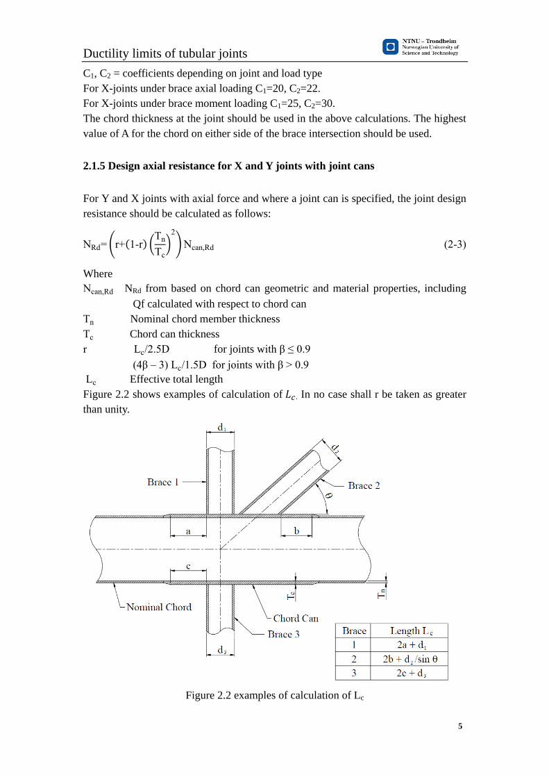
2.1.5 Design axial resistance for X and Y joints with joint cans
For Y and X joints with axial force and where a joint can is specified, the joint design
resistance should be calculated as follows:
NRd=(r+(1-r) (Tn
Tc)2
)Ncan,Rd (2-3)
Where
Ncan,Rd NRd from based on chord can geometric and material properties, including
Qf calculated with respect to chord can
Tn Nominal chord member thickness
Tc Chord can thickness
r Lc/2.5D for joints with β ≤ 0.9
(4β – 3) Lc/1.5D for joints with β > 0.9
Lc Effective total length
Figure 2.2 shows examples of calculation of 𝐿𝑐 . In no case shall r be taken as greater
than unity.
Figure 2.2 examples of calculation of Lc
Ductility limits of tubular joints
6
2.2 NORSOK standard N-004 for ductility
It is a fundamental requirement that all failure modes are sufficiently ductile such that
the structural behavior will be in accordance with the anticipated model used for
determination of the responses. In general all design procedures, regardless of
analysis method, will not capture the true structural behavior. Ductile failure modes
will allow the structure to redistribute forces in accordance with the presupposed
static model. Brittle failure modes shall therefore be avoided or shall be verified to
have excess resistance compared to ductile modes, and in this way protect the
structure from brittle failure.
The following sources for brittle structural behavior may need to be considered for a
steel structure:
1) Unstable fracture caused by a combination of the following factors:
- Brittle material;
- A design resulting in high local stresses;
- The possibilities for weld defects.
2) Structural details where ultimate resistance is reached with plastic deformations
only in limited areas, making the global behavior brittle, e.g. partial butt weld loaded
transverse to the weld with failure in the weld.
3) Shell buckling.
4) Buckling where interaction between local and global buckling modes occur.
NORSOK standard N-004 Rev. 2, October 2004
NORSOK standard Page 18 of 287
In general a steel structure will be of adequate ductility if the following is satisfied:
1) Material toughness requirements are met, and the design avoids a combination of
high local stresses with possibilities of undetected weld defects.
2) Details are designed to develop a certain plastic deflection e.g. partial butt welds
subjected to stresses transverse to the weld is designed with excess resistance
compared with adjoining plates.
3) Member geometry is selected such that the resistance does not show a sudden drop
in capacity when the member is subjected to deformation beyond maximum resistance.
An unstiffened shell in cross-section class 4 is an example of a member that may
show such an unfavorable resistance deformation relationship. For definition of
cross-section class see NS 3472 or NSENV 1993 1-1.
4) Local and global buckling interaction effects are avoided.
2.3 Nonlinear finite element analysis
Non-linear analysis methods have been available for more than 40 years, but it is first
during the last decade that these methods have found broad application for offshore
structures. This is particularly true when it comes to assessment of existing structures.

Ductility limits of tubular joints
7
Modern codes for offshore structures allow the use of nonlinear methods and are also
giving some guidance on how to execute the analyses [2]
. Nevertheless, performing
non-linear analysis involves many new and demanding challenges both for the analyst
and also for those that are reviewing the work.
3. Characteristic behavior of tubular joints
and theoretical basis of the thesis
3.1 Brief introduction[3]
The characteristics of load-deformation of X-joints are different under different
loading conditions, which represents the input for nonlinear spring models in the
frame analysis. Before the ultimate joint strength is reached a bilinear model is
employed in consistence with the plastic limit load approach for all loading conditions.
For brace axial compression, a re-development of the joint strength occurs at a large
deformation level due to the direct contact of the compression braces which are
observed in the BOMEL 2D and 3D frame tests. The re-gained strength level equals
the brace yield strength, corresponding to δy = 0.5d0.
The strength re-development’s initialization depends on the 𝛽 ratio, as shown in figure
3.1, which defines 𝛿𝑖 at the initial contact of the two braces. For joints with
large 𝛽 ratios, however 𝛿i becomes impractically small (𝛿𝑖= 0 for 𝛽= 1.0). Since the
large 𝛽 joint can undergo certain deformation before the two braces contact one
another, 𝛿 i takes the maximum of 0.1d0 and 0.5d0sin(cos-1𝜓 ). The 0.1d0 is a
suggested value in the USFOS joint recommendations (USFOS, 2003).
Figure 3.1 Deformation level at the initial contact of two braces for X-joints under
brace axial compression.

Ductility limits of tubular joints
8
This is confirmed by an isolated joint analysis by ABAQUS. Contact algorithm is
implemented in the analysis so that no self-penetration of the chord inner surface is
allowed. The deformation mode at the end of the analysis is shown in Figure 3.2
together with the load deformation response. Once the two braces are in contact, the
joint strength will go fast towards the yield strength.
For brace axial tension, the reduction in strength beyond the ultimate load level
accounts for the fracture failure in the joint at a large deformation level. As USFOS
recommends, the crack initiation is assumed to be at a deformation level of 0.1d0. The
joint strength beyond the first crack depends on the extent of crack in the joint. An
estimation of the cracked joint strength is based on the 30% of the intact cross-section
area, or, Pcr = 0.3Pu, which is arbitrary to simulate the crack failure. It is required by
numerical analyses in USFOS that a reduction is needed in the load deformation curve.
These load-deformation parameters are investigated in the sensitivity study.
Figure 3.2 X-joint: (a) deformation mode; and (b) load-deformation curve[4]
.
Figure 3.3 Bilinear load-deformation characteristics for nonlinear spring elements [5]

Ductility limits of tubular joints
9
The load-deformation relation re-plotted in Figure 3.3 can be evaluated with reference
to the bilinear model. The load level PE corresponding to the limit of elasticity is
assumed to be cPu, where c defines the ratio of the elastic limit load over the plastic
limit load and remains less than 1.0. Since the ultimate joint strength in the current
study is based on the plastic limit load at which Wp
WE=3.0. The total work
(WT=WP+WE) equals (k0= cPu/δE):
WT=1
2
c2Pu2
k0+1
2(1+c)Pu(δu-δE)=
1
2
Pu2
k0[c2+(1+c)c(
δu
δE -1)] (3-1)
WE=1
2
Pu2
k0 (3-2)
WT
WE
=c2+(c+c2) (δu
δE-1)=4 (3-3)
δu=c+4
c+1
Pu
k0 (3-4)
or
c=4Pu-k0δu
k0δu-Pu (3-5)
Based on Equation 3-1 to 3-5, δushould satisfy the conditions as denoted in equation
below, since 0 < c < 1.
Pu
0.4k0<δu<
Pu
0.25k0
The secant stiffness of the joint at ultimate strength level is thus between 0.25k0 and
0.4k0.
3.2 Initial Joint Stiffness k0
From the initial steps of the FE analysis we obtain the initial joint stiffness, where the
stress-state in the joints remains essentially elastic. The initial joint stiffness is cast in
a non-dimensional format based on the non-dimensional strength and deformation
parameters adopted in the current study, and the joint stiffness follows a power
function of 𝛾. The functions are shown in Equation 3-6 and 3-7[6]
.
k0=Psinθ/fyt0
2
δ/t0=P
δ
d0sinθ
fyt02 (3-6)
k0(γ,β)=f1(β)γf2(β) (3-7)
Table 3.1 X-joint stiffness for different brace loads[7]
Loading k0 (P
δ
d0sinθ
fyt02 )or(
M
ϕ
sinθ
fyt02d)
FE/k0
Mean Standard No. of

Ductility limits of tubular joints
10
Deviation data
Axial 1185γ(0.8β2+0.15β-0.4) 1.00 0.08 40
IPB (410β2-337β+91)γ(-0.46+1.15) 1.00 0.04 15
OPB 123β(1.8+0.095γ)
γ(2.9β2-4.4β+2.5)
1.02 0.05 15
The coefficients in Equation 3-6 and 3-7 are assumed to depend on 𝛽, and determined
by regression analysis. In Eq. 3-7, f1(β) and f2(β) follow the polynomial relationship.
The stiffness formulation k0 is tabulated in Table 3.1. The statistical comparison with
respect to FE data is incorporated in the same table.
3.2 Ultimate Joint Strength
The ultimate strength equation is simplified based on the exact ring model solution
proposed by van der Vegte (1995)[8]
. The X-joint strength formulation is shown in
Equation 3-8 for brace axial compression, axial tension, IPB and OPB respectively.
Modifications have been included to incorporate the dependence for thick-walled
joints.
Pusinθ
fyt02=
p1
(1-p2βγ)γ(p3+p4β) (3-8)
Mu,ipbsinθ
fyt02d1
=p1βp2γp3 (3-9)
Mu,opbsinθ
fyt02d1
=p1γf(β) (3-10)
Table 3.2 X-joint strength formulation for different brace loads
Loading Pusinθ
fyt02 or
Musinθ
fyt02d1
FE/k0
Mean Standard
Deviation
No. of
data
Axial 8.8
(1-0.4βγ)γ(-0.2+0.56β) 0.98 0.08 51
IPB 3.1βγ0.65 1.00 0.07 15
OPB 3.8γ0.53β2.4
0.99 0.08 15
Table 3.2 shows the final equations for X-joints obtained using nonlinear regression
analyses. Table 3.2 also shows the statistical comparison of the proposed equation and
FE data. The representation for X-joints under tension is based on the ultimate joint

Ductility limits of tubular joints
11
strength instead of the strength corresponding to the first crack, since fracture failure
does not become dominant until it achieves a large deformation level, which is
different from ISO formulation.
3.3 Coefficients c and δu
To form a complete bilinear model, the coefficient c needs to be determined to
evaluate PE (= cPu) and ME (= cMu). For X-joints, a convenient value of 0.8 is
assumed for c under all loading conditions.
Table 3.3 Comparison of 𝜹𝒖by Eq. 8.4 and FE results for X-joints
Loading No. of data
δuor ϕu(FE) /δu or ϕ
u(Eq.
3-4 & 3-5)
Mean Standard Deviation
Axial 40 0.98 0.08
IPB 15 1.00 0.07
OPB 15 0.99 0.08
The joint deformation δu is calculated using Equation 3-4 and compared to the joint
deformation obtained from the FE analysis. Table 8.4 shows a good agreement in the
deformation level between Equation 3-4 and the FE data, which indicates the
appropriateness of the c value assumed.
3.3 MSL Joint behavior and ductility limits [9]
3.3.1 General
The current joint capacity check included in USFOS covers simple tubular joint and is
based on capacity formulas and description of the joint behavior developed during the
MSL Joint Industry Projects. In addition to the original MSL formulations, code
variants from Norsok, ISO and API are also implemented.
3.3.2 MSL variants
The MSL Joint Industry Projects developed several sets of capacity formulas based on
a large database of laboratory test results.

Ductility limits of tubular joints
12
The original MSL versions include
•Mean Ultimate
•Characteristic Ultimate
•Characteristic First Crack
Mean Ultimate represents the statistical mean failure of the joints tested (top of the
force-displacement curve, "the most probable failure load").
Characteristic Ultimate is based on the same data, but the as the title say, the capacity
is reduced in order to account for the spreading in the test results.
Characteristic First Crack is in most cases equal to "Characteristic Ultimate" but is
further reduced in some cases in order to avoid degradation of the joint for repeated
loading. This version is recommended for structures subjected to repeated load actions,
e.g. wave loading.
3.3.3 Code variants
Note that the first crack characteristic capacity equations in the code variants are
implemented in USFOS excluding the safety factors given in the codes. The
additional safety level required by the code for the various limit states analyzed must
in USFOS be included on the load side (by increasing the applied loads).
The MSL capacity check formulas have been adopted and adjusted by Norsok and
ISO. The code variants are based on the MSL First Crack capacity formulas. The (Qu)
expressions are nearly identical, but the correction factor for chord utilization differs
from MSL. Also the interaction between axial force, in-plane and out-of-plane
bending differs. The code variants put more weight on the out-of plane bending
component.
The formulas are also based on the MSL database, however, the database used to
develop the latest joint capacity equations for API RP2A are extended using results
from FE analyses. API RP2A (21st edition) is currently (2009) the most updated code
with respect to joint capacity.
In this paper Norsok-004 is discussed and the other codes are neglected.
3.3.4 Joint P-D curves
The following expressions show the original MSL proposed relationship between the
joint force/moments and joint displacements/rotations.

Ductility limits of tubular joints
13
P=ϕPu (1-A [1- (1+1
√A) exp(-B
δ
ϕQfFyD
)]
2
) (3-11)
M=ϕMu (1-A [1- (1+1
√A) exp(-B
θ
ϕQfFy)]
2
) (3-12)
Table 3.4 Coefficients A and B
Joint
Type Load Type
Coefficient
A B
X
Compression ((γ-4)sin3θ) /62 600β+13500
Tension 0.001 12000𝛽
+ 1200
IPB 0.001 9700𝛽 + 6700
OPB 0.001 8600𝛽 + 1200
Where γ and β are the parameters shown in section 2.1.1.
3.3.5 MSL Ductility limits
The MSL proposed ductility limits of X-joints for axial deflection are:
Mean:
δ
D=0.13-0.11β
Characteristic:
δ
D=0.089-0.075β
In USFOS, the ductility limit is implemented by reducing the axial joint capacity to a
small number for deformations larger than the ductility limit. No formulations are
identified for mean and characteristic fracture criteria related to other degrees of
freedom.
From the limits it is seen that the ductility limits are very conservative. It is no more
than 0.13 times the out diameter. While during the analysis by ABAQUS, it is seen
that the joints can deform much larger than the limit before they reach the yield stress
limit, which will be shown later.
Ductility limits of tubular joints
14
3.4 The BWH instability criterion[10]
3.4.1 Introduction
When exploring the limits of metal sheets it is important to give reasonable prediction
of fracture. This is true for metal forming processes and in crash worthiness analyses
where failure may reduce the resistance of a structure significantly. In industrial
forming processes, the Keeler–Goodwin approach, see Keeler and Backhofen
(1964)[11]
and Goodwin (1968)[12]
, has for many years been the dominating method to
estimate failure. In this method, the principal strains (ε1,ε2) at incipient plastic
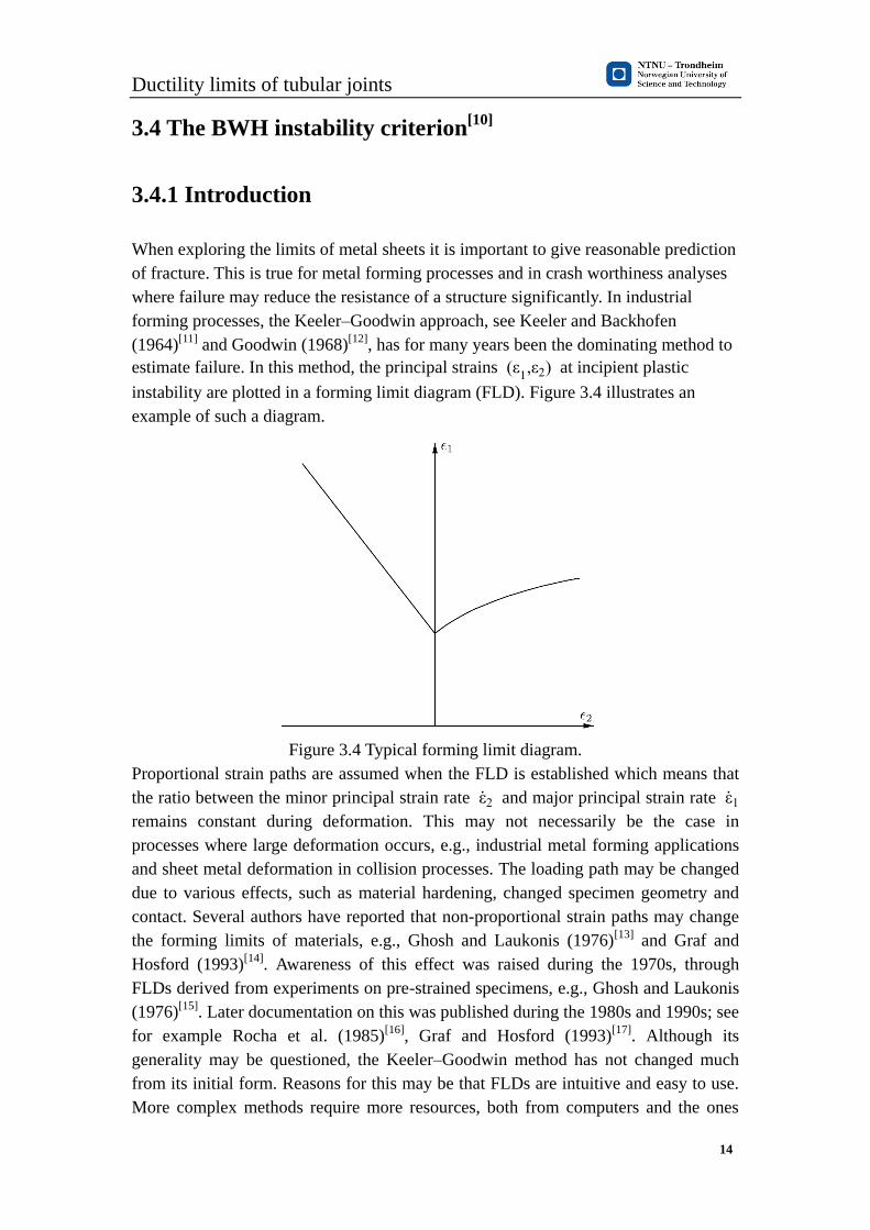
instability are plotted in a forming limit diagram (FLD). Figure 3.4 illustrates an
example of such a diagram.
Figure 3.4 Typical forming limit diagram.
Proportional strain paths are assumed when the FLD is established which means that
the ratio between the minor principal strain rate ε2 and major principal strain rate ε1
remains constant during deformation. This may not necessarily be the case in
processes where large deformation occurs, e.g., industrial metal forming applications
and sheet metal deformation in collision processes. The loading path may be changed
due to various effects, such as material hardening, changed specimen geometry and
contact. Several authors have reported that non-proportional strain paths may change
the forming limits of materials, e.g., Ghosh and Laukonis (1976)[13]
and Graf and
Hosford (1993)[14]
. Awareness of this effect was raised during the 1970s, through
FLDs derived from experiments on pre-strained specimens, e.g., Ghosh and Laukonis
(1976)[15]
. Later documentation on this was published during the 1980s and 1990s; see
for example Rocha et al. (1985)[16]
, Graf and Hosford (1993)[17]
. Although its
generality may be questioned, the Keeler–Goodwin method has not changed much
from its initial form. Reasons for this may be that FLDs are intuitive and easy to use.
More complex methods require more resources, both from computers and the ones

Ductility limits of tubular joints
15
applying them.
A simple alternative to strain based FLDs is stress based FLDs. Such diagrams were
first presented by Arrieux et al. (1982)[18]
, and later by Stoughton (2000, 2001)[19]
,
Stoughton and Zhu (2004)[20]
and Wu et al. (2005)[21]
. The idea is that stress based
criteria remains more or less unaffected by altered strain paths. Furthermore, the
nature of this type of formulation is simple and easily implemented into a finite
element (FE) code.
The BWH criterion is meant to offer a simplified way to estimate the onset of local
necking. The verification of the BWH criterion is carried out in two separate series of
analyses. The first one is a set of analytical considerations, which is compared with
FLDs found in literature. The second set of analyses is performed numerically using
the finite element code LS-DYNA, see Hallquist (2007a, b)[22]
. The finite element
simulations are further compared with benchmark tests (large scale bulge tests)
provided by Tornqvist (2003)[23]
.
3.4.2 The BWH instability criterion
The forming limit diagram, as it is most often presented, is an intuitive way of
displaying the limits of materials. However, as it has been highlighted, it is only
strictly valid for proportional straining, i.e., the strain rate ratio β=ε2/ε1 remains
constant. Ghosh and Laukonis (1976)[24]
and Graf and Hosford (1993)[25]
have shown
that for non-linear strain paths, the FLD may change. One simplified way of
circumventing this problem is to adopt stress based forming limit curves (FLC). This
methodology has been strongly argumented for by Stoughton, see for example
Stoughton (2000, 2001)[26]
and Stoughton and Zhu (2004)[27]
. Stresses can be directly
coupled to the plastic strain rates through the relations between the strain rates and the
conditions for yielding and plastic flow. If the yield function and the potential for
plastic flow are assumed identical, the relations between strain rates and stresses can
be found from the associated flow rule
εij=λ∂f
∂σij (3-13)
where εij and σij denotes plastic strain rate and stress tensor on index form, k is the
plastic multiplier, and f describes the yield function. If J2 flow theory and plane
stress conditions are assumed, the relation between the strain rate ratio b and the
principal stresses σ1 and σ2 can be expressed as
α=σ2
σ1=1+2β
β+2 (3-14)
Note that only for plastic strains is this relation valid. Elastic strains are neglected,
which is reasonable since plastic strains are much larger. In Figure 3.5, an example of

Ductility limits of tubular joints
16
a strain based FLD (a) and a stress FLD (b) is shown. The difference between these is
that the stress based FLC remains fixed in the stress space for non-linear strain paths,
while the strain based FLC may change for various combinations of non-proportional
straining.
3.4.2.1 Hill’s local necking criterion
Hill (1952)[28]
proposed a criterion for local necking in the negative β regime. He
assumed that a local neck will form with an angle ϕ to the direction of the major
principal stress. Within this neck, the strain increments along the narrow necking band
will be zero. The orientation of the neck may be expressed as ϕ=tan-1 (1/√-β), which
yields rational results only for negative values of b. At the instant a neck is formed,
the effects from strain hardening and the diminution in thickness balance each other
exactly. This means that the fractions within the material reach a maximum value at
the point of local necking. This gives traction increments equal to zero, dT1=0, at the
point of necking, which leads to the following local necking criterion
dσ1
dε1=σ1(1+β) (3-15)
Assuming that the material stress–strain curve can be represented by the power law
expression, σeq=Kεeqn , where (K, n) are material parameters and (σeq, εeq) are the
equivalent stress and strain, and that proportionality between stress rates and stresses
can be assumed, i.e.,
α=σ2
σ1=σ2
σ1 (3-16)
the equivalent strain at local necking can be expressed as
εeq=2n
√3
√β2+β+1
1+β (3-17)
Figure 3.5 Forming limit diagrams in (a) strain space, (b) stress space. Both figures

Ductility limits of tubular joints
17
illustrate the same materials. Note that the figure (b) is normalized by the powerlaw
parameter K in σeq=Kεeqn , where (σeq, εeq) are the equivalent stress and strain
If proportional straining is assumed, the familiar strain based Hill’s expression
appears
ε1*=
ε1
1+β (3-18)
Here ε1 is equal to the power law exponent n, although measured values may
sometimes yield better correlation with experiments. As equation Eq. 3-18 is based on
proportionality it has limited use. Alternatively, a path independent stress based FLC
may be found directly from Eq. 3-17 and the power law expression. This gives the
equivalent stress at local necking (note that also here refers to the power law exponent
n)
εeq=
(
2ε1
√3
√β2+β+1
1+β
)
n
(3-19)
This results in the following major principal stress
σ1=2K
√3
1+β2
√β2+β+1
(2
√3
ε1
1+β√β2+β+1)
n
(3-20)
A similar derivation has been shown by Stoughton and Zhu (2004)[29]
.
3.4.2.2 The Bressan–Williams shear instability criterion
Hill’s local necking criterion yields only rational results for negative β values. In the
positive regime, other methods of estimating the onset of local necking are needed. A
popular solution to this goes through the methodology established by Marciniak and
Kuczynski (1967) (M–K)[30]
. This procedure introduces pre-existing defects within
the material, which trigger local necking. The defects are often introduced as a groove
within a material element. During deformation, the strain field is solved incrementally.
Local necking is initiated once the material within the groove starts to strain at a
significantly higher rate than the surrounding material and the strain rate ratio b
within the emerging neck approaches zero (plane strain). The M–K method describes
in a physical way the initial stage of local necking and as for stress based approaches,
it does handle non-proportional straining. The drawback, however, is that it becomes
computationally demanding if used in finite element analyses. Either one has to apply
a high number of small elements in order to include small imperfections, or the M–K
procedure needs to be introduced into each finite element. Hence, a much simpler
stress based instability criterion known as the Bressan–Williams criterion (BW) is
adopted, Bressan and Williams (1983)[31]
. Contrary to the M–K method, the BW

Ductility limits of tubular joints
18
criterion may be solved analytically and can be used for failure estimation with
reasonable precision at a low cost.
In plasticity, the main mechanism of deformation comes from slip arising from shear
on certain preferred combinations of crystallographic planes. Furthermore, it has been
observed by experiments that failure planes in sheet metal lie close to the direction of
maximum shear stress, see Bressan and Williams (1983)[32]
. It is therefore reasonable
to assume that the instability may take place before any visual signs of local necking.
Thus, a shear stress based instability criterion may well be useful in estimating the
point of local necking. As presented by Bressan and Williams (1983), the BW
criterion has a simple expression and has been applied with good results. The basis for
the BW expression follows three basic assumptions. First of all, the shear instability is
initiated in the direction through the thickness at which the material element
experiences no change of length. This indicates a critical through thickness shear
direction. Secondly, the instability is triggered by a local shear stress which exceeds a
critical value. This means that the initiation of local necking is described as a material
property. Finally, elastic strains are neglected. This is reasonable since the elastic
strains are small compared to the plastic strains at local necking.
From Fig. 3, and from the assumptions above, a mathematical formulation for the BW
criterion can be found. As illustrated in Figure 3.6a, the inclined plane through the
element thickness at which shear instability occurs (indicated by the plane normal xn)
forms an angle π/2-θ to the shell plane. The material experiences zero elongation in
this direction, indicating that εt=0. This gives the following relation between the angle
of the inclined plane and the principal strain rates
εt= ε1+ ε2
2+ ε1- ε3
2cos 2 (θ+
π
2)=0 (3-21)
Where cos 2(θ+π/2)= cos 2θ, which further gives
cos 2θ = ε1+ ε3
ε1- ε3 (3-22)
Figure 3.6 (a) Local shear instability in a material element. Note that no elongation

Ductility limits of tubular joints
19
takes place in the xt direction. (b) Shows the stress components in a Mohr’s circle.
Assuming plastic incompressibility, ε3=- ε1(1+β), the angle θ can be found as a
function of the ratio β
cos 2θ =-β
2+β (3-23)
The corresponding stress state can be obtained from the rules of stress transformation,
or simply by drawing up Mohr’s circle, Figure 3.6b. This gives the following relation
between the inclined plane and the stresses involved
τcr=σ1
2sin 2θ (3-24)
where τcr is the critical shear stress. Finally, equations may be combined into the
expression which gives the BW criterion
σ1=2τcr
√1- (β2+β
)2
(3-25)
A similar derivation is given by Brunet and Clerc (2007)[33]
. Bressan and Williams
initially suggested calibration either from uniaxial tensile tests or biaxial tests.
Another alternative may be calibration at plane strain, β= 0, through notched
specimens or simply from Hill’s analysis. If the BW criterion is calibrated from Hill’s
expression at plane strain, the critical BW shear stress takes the following form
τcr=1
√3K (
2
√3ε1)
n
(3-26)
Also here, ε1 is equal to the power law exponent n.
3.4.2.3. The Bressan–Williams–Hill criterion
The BW criterion was initially intended for the positive quadrant of the FLD, but the
mathematical expression is also valid for negative values. However, as the strain rate
ratio becomes negative, the validity of the BW criterion becomes questionable. Hence,
in order to cover the full range of β, the Hill and BW criteria have been combined into
one criterion, from now on referred to as the BWH criterion. Formulated in terms of
the strain rate ratio, β, the criterion reads
σ1=2K
√3
1+12β
√β2+β+1
(2
√3
ε1
1+β√β2+β+1)
n
, β≤0

Ductility limits of tubular joints
20
σ1=2K
√3
(2
√3ε1)
n
√1- (β2+β
)2
, otherwise
The BWH criterion is illustrated in both strain and stress space in Figure 3.5 for
various hardening exponents, n.
3.5 Introduction of Nonlinear Analysis[34]
3.5.1. General
Structural analysis, the finite element method included, is based on the following
principles:
Equilibrium (expressed by stresses)
Kinematic compatibility (expressed by strains)
Stress-strain relationship
When doing linear analysis it is assumed that displacements are small and the material
is linear and elastic. When the displacements are small, the equilibrium equations can
be established with reference to the initial configuration, which means that the strains
and displacement gradients (derivatives) have linear relation corresponding to
Hooke’s law.
However when the ultimate strength of structures such that buckle and collapse is to
be calculated, small displacements and linear material assumptions are no longer
available and accurate. If the change of geometry is accounted for, when establishing
the equilibrium equations and calculating the strains from displacements, a
geometrical nonlinear behavior is accounted for. Analogously, material nonlinear
behavior is associated with nonlinear stress-strain relationship.
Nonlinearity may be also related to the boundary condition, i.e. when a large
displacement leads to contact. Boundary non-linearity occurs in most contact proble-
ms, in which two surfaces come into or out of contact. The displacements and stresses
of the contacting bodies are usually not linearly dependent on the applied loads. This
type of non-linearity may occur even if the material behavior is assumed linear and
the displacement are infinitesimal, due to the fact that that the size of the contact area
is usually not linearly dependent on the applied loads, i.e. doubling the applied loads
does not necessarily produce double the displacement. If the effect of friction is incl-

Ductility limits of tubular joints
21
uded in the analysis, then slick-slip behaviour may occur in the contact area which
adds a further nonlinear complexity that is normally dependent on the loading history.
There are several areas where nonlinear stress analysis may be necessary:
Direct use in design for ultimate and accidental collapse limit states. Modern
structural design codes refer to truly ultimate failure modes and not only first
yield and analogous modes.
Use in the assessment of existing structures whose integrity may be in doubt due
to (a) visible damage (crack, etc.) concern over corrosion or general ageing. The
above will largely relate to the ultimate limit state because, in many cases, the
serviceability limit state will already have been exceeded and yet key question
still remain such as: Is the structure safe? Should it be repaired and if so, how will
any proposed strengthening work? Can it be kept in service for a little time
longer?
Use to help to establish the causes of a structural failure.
Use in code development and research: (a) to help to establish simple ‘code
based’ methods of analysis and design, (b) to help understand basic structural
behavior and (c) to test the validity of proposed ‘material models’.
With the new generation of inexpensive yet powerful computers, solution cost is no
longer the major obstacle it has been. However, the complexity of nonlinear stress
analysis still remains to provide the ‘expert’ as well as the unwary novice with many
headaches.
Nonlinear analyses are applied in all the ways mentioned above. However, a signify-
cant increase in the use of nonlinear stress analyses in the assessment of existing stru-
ctures is envisaged and eventually in the direct design of more routine structures. This
will occur as hardware becomes cheaper and faster and software becomes more robust
and user-friendly.
It will simply become easier for an engineer to apply direct analysis rather than code
based charts. However, problems will arise because the latter often include ‘fiddle
factors’ relating to experience, uncertainty, etc. The advent of more computer-based
analysis procedures will lead to the need for a ‘surrounding’, probably computer
based, 'code' to incorporate the ‘partial factors’ including those factors (often now
hidden) relating to the degree of uncertainty of the analysis. The analysis would have
to be directly embedded in a statistical reliability framework.
3.5.2 Nonlinear material behavior
A material is called nonlinear if stresses σ and strains ε are related by a strain

Ductility limits of tubular joints
22
dependent matrix rather than a matrix of constants. Thus the computational difficulty
is that equilibrium equations must be written using material properties that depend on
strains, but strains are not known in advance. Plastic flow is often a cause of material
nonlinearity. The present section deals with formulation of elastic-plastic problems by
considering the one dimensional case.
Assume that yielding has already occurred, and then a strain increment dε takes place.
This strain increment can be regarded as composed of an elastic contribution dεe and
a plastic contribution dεpso that dε=dεe+dεp. The corresponding stress increment can
be written in various ways
dσ=Edεe=E(dε-dεp) dσ=Etdε and dσ=H'dεp
Where H' is called the plastic tangent modulus as given by ∂σ/∂εp. Substitution of
the first and third into the second yields
H'=1
1Et-1E
or Et=E (1-E
E+H') (3-27)
where Et is the tangent modulus. When written in this form, the expression for Et is
similar to a more general expression used for multiaxial states of stress. If E is finite
and Et=0, then H'=0, and the material is called “elastic-perfectly plastic”.
Figure 3.7 characteristic features of one-dimensional stress-strain relationships.
A summary of elastic-plastic action in uniaxial stress is as follows:
1) The yield criterion states that yielding begins when |σ| reaches σ , where in
practice σ is usually taken as the tensile yield strength. Subsequent plastic
deformations may alter the stress needed to produce renewed or continued yielding;
this stress exceeds the initial yield strength σ if Et>0.
2) A hardening rule, which describes how the yield criterion is changes by the history
of plastic flow. For example, imagine that the material first has been loaded to point B
Ductility limits of tubular joints
23
and then unloading occurs from point B to point C in Figure 3.7a. With reloading
from point C, response will be elastic until σ>σB, when renewed yielding occurs.
Assume then that unloading occurs from point B and progresses into a reversed
loading as shown in Figure 3.7b. If the yielding is assumed to occur at |σ|=σB the
hardening is said to be isotropic. However, for common metals, such a rule is in
conflict with the observed behavior that yielding reappears at a stress of approximate
magnitude σB-2σ when loading is reversed. Accordingly, a better match to observed
behavior is provided by the “kinematic hardening” rule, which (for uniaxial stress)
says that a total elastic range of 2σ is preserved.
3) A flow rule can be written in multidimensional problems. It leads to a relation
between stress increments dσ and strain increments dε. In uniaxial stress this relation
is simply dσ=Etdε, which describes the increment of stress produced by an increment
of strain. Note, however, that if the material has yet to yield or is unloading,
then dσ=Edε, (e.g., Figure 3.7a, complete unloading from point B leads to point C and
a permanent strain εp).
3.5.3 Solution techniques
While in linear analysis the solution always is unique, this may no longer be the case
in non-linear problems. Thus the solution achieved may not necessarily be the
solution sought.
The resultant of internal forces can be expressed as
Rint=∑(ai)TSi
i
(3-28)
and the total equilibrium can be expressed as
Rint=R (3-29)
Hence, the equations that need to be solved are formulated in terms of a total and an
incremental equation of equilibrium
∑(ai)TSi
i
=R (3-30)
KI(r)dr=dR (3-31)
For a given external load, R the displacement vector r is sought.
Various techniques for solving these non-linear problems exist. Herein three types of
methods will be briefly described, namely:
Euler-Cauchy method)
(Newton-Raphson method)
In this paper, these methods are not considered, but the advanced solution is
considered.

Ductility limits of tubular joints
24
3.5.4 Advanced solution procedures
General
The solution procedure described so far are combination of incremental load coupled
with full or modified Newton-Raphson iterations. Because the plastic flow rules are
incremental in nature elasto-plastic problems should strictly be solved using small
incremental steps. For, no matter how accurately flow rules and keeping on the yield
surface may be satisfied within an increment, the solution is only in equilibrium at the
end of each increment after equilibrium iterations. However, often acceptable
solutions can be obtained with large steps.
Although incremental-iterative techniques provide the basis for most nonlinear finite
element computer programs, additional sophistications are required to produce
effective, robust solution algorithms. An extensive of more refined methods are
discussed e.g. in Chapter 9 of Crisfield (1991). In this section a brief review of such
methods is given.
In the present section emphasis will be placed on arc-length techniques for solving
these problems. Prior to their introduction, analysts either used artificial springs,
switched from load to displacement control or abandoning equilibrium iteration in the
close vicinity of the limit point. In relation to structural analysis, the arc-length
method was originally introduced by Riks [1972] and Wempner [1971] with later
modifications being made by a number of authors.
The limit point represents the ultimate strength. There are several reasons:
i) In many cases it may be important to know not just the collapse load, but whether
or not this collapse is of a “ductile” or “brittle “nature.
ii) The structure with the characteristic displayed in Fig. 12.22 may represent a
component in structure. The ultimate behavior of a redundant structure consisting of
such components would depend upon the post-ultimate beyond limit point, L)
behavior of the component.
Method
As a starting point the global equilibrium equation is written as:
g(r, λ)=Rint(r)-λRref= (3-32)
where Rref is a fixed external load vector and the scalar λ is a load level parameter.
Equation above defines a state of “proportional loading” in which the loading pattern
is kept fixed. Non-proportional loading will be briefly mentioned later in this section.
The essence of the arc-length method is that the solution is viewed as the discovery of
a single equilibrium path in a space defined by the nodal variables, r and the loading
parameter, λ. Development of the solution requires a combined incremental (also
called predictor) and iterative (also called corrector) approach.
Ductility limits of tubular joints
25
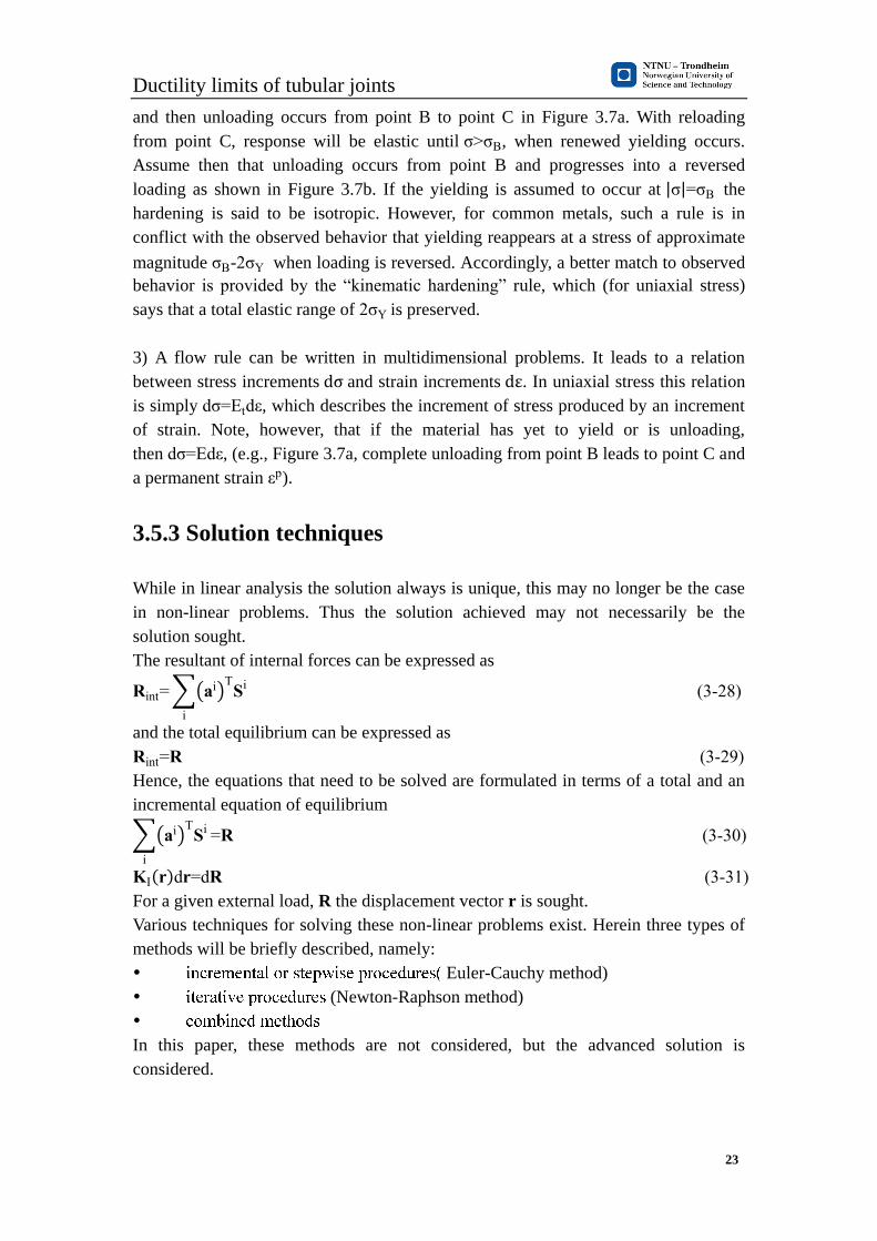
Many of the materials (and possibly loadings) of interest will have path-dependent
response. For these reasons, it is essential to limit the increment size. The increment
size is limited by moving given distance along the tangent line to the current solution
point and then searching for equilibrium in plane that passes through the point thus
obtained and that is orthogonal to the same tangent line (Figure 3.8c).
In figure 3.8c the arc-length control strategies in the solution of nonlinear equations
are illustrated and compared with load and displacement control. For instance if load
incrementation is applied, the iterations are carried out to correct the displacements.
When the arc-length method is applied the iterations are carried out with respect to
both the load and displacements.
Figure 3.8Geometric representation of different control strategies of non-linear
solution methods for single d.o.f.
a) Load control, b) state control, c) arc-length control
The arc length is formulated as an additional variable involving both the load and
displacement. The increment in the load-displacement space can be described by a
displacement vector r and a load increment parameter λ, such that R = λRref.
This formulation results in an additional equation to be solved. The advantage of the
extra equation is that the solution matrix never becomes ‘singular’ even at the limit
points. Therefore, the solution matrix is re-assembled with N+ 1 variable, where N is
the total number of the variables (degrees of freedom) of the system. However, the
disadvantage is that the solution matrix becomes unsymmetric in some formulations,
which may incur an increase in computing time and/or computer storage, particularly
for very large problems. First the increment (predictor) from the “First point” is made
along the tangent. Then, this solution is corrected iteratively to reach the “Second
point” and so on.
Several methods exist to obtain the arc length, for example by making the iteration
path follow a plane perpendicular to the tangent of the load-displacement curve, as
shown in Figure 3.9. Alternatively, instead of a normal plane, more sophisticated
paths such as spherical or cylindrical planes can be followed, and the solution matrix
can be manipulated to become symmetric (see, for example, Crisfield [1991]).

Ductility limits of tubular joints
26
Figure 3.9: Schematic representation of the arc-length technique.
A geometrical interpretation of the incremental iterative approaches by Riks
Wempner and Ramm is sketched in Figure 3.10. While in Ramm’s method the
iterative corrector is orthogonal to the current tangential plane during the iteration, it
is orthogonal to the incremental vector ( r0, r0)in the Riks-Wempner methods.
Figure 3.10 Arc-length control methods (Crisfield, 1991)
An alternative iterative method is so-called orthogonal trajectory iterations (Fried,
1984). the first step in this method can be illustrated by reference to Figure 3.8. The
first iteration is then assumed to be orthogonal to the vector S’P’ instead of SP. The
resulting iterative solution will appear as shown in Fig. 12.33.
Haugen (1994) found that this method was more efficient than the normal plane
iterations.

Ductility limits of tubular joints
27
Figure 3.11 Arc-length method with orthogonal trajectory iterations.
Automatic incrementation
To achieve computational efficiency the load increment should be chosen depending
upon the degree of nonlinearity of the problem. Methods have been established based
on the curvature of the nonlinear path (den Heijer and Rheinboldt, 1981) or the
so-called current stiffness parameter (Bergan et al, 1978):
Spi= r1
T R1
λ12
λi2
riT Ri
(3-33)
Spi refers to increment No.i.
The initial value of Spi (Sp
1) is 1.0. For stiffening system it will increase. For softening
system it will decrease. If Spi changes sign the sign of the increment should be changed.
Numerical experiments show that nearly the same numbers of iterations are requested
to restore equilibrium when the increments were chosen according to the approach of
Bergan et al.( 1978).
Ramm (1981) proposed another approach for estimating the necessary increment λ
(load incrementation) or λ (for arc-length method). The new arc-length, ln is
obtained by
ln= l0 (Id
I0)1/2
(3-34)
where 0 is the “old” arc-length, and Id and I0 are the desired number of iterations

Ductility limits of tubular joints
28
(given as input) and the number of iterations when the old arc-length was used. This
approach requires a suitable estimate of the initial arc-length.
An alternative tactic is to apply load incrementation for early increments and switch
to arc-length control once a limit point is approached.
The current stiffness parameter can be used to decide the switch from load
incrementation (or displacement control) to the arc-length method. An alternative
indicator of when the limit point is approached is the check of negative values on the
diagonal of the incremental stiffness matrix, i.e. negative pivot elements in the
solution algorithm.
In particular the current stiffness parameter may be used to control the solution
strategy at limit points or bifurcation points. Alternative changes may be made when
the current stiffness is below a limit value, namely
the sign of the incrementation is changed
iteration may be suppressed and a simple incrementation may be used. Iterations
are then resumed when 𝑖
increases beyond a specific limit (see Figure 3.12).
Figure 3.12 Possible choice of solution algorithm for a problem with limit point
Non-proportional loading
The solution procedures in this chapter have been based on the equilibrium

Ductility limits of tubular joints
29
relationship of (12.101) which implies a single loading (or displacing) vector, Rref, is
proportionally scaled via λ. For many practical structural problems, this loading
regime is too restrictive. For example, we often wish to apply the “dead load” or
“self-weight” and then monotonically increase the environmental load. Even more
general load conditions may be required. Fortunately, many such loading regimes can
be applied by means of a series of loading sequences involving two loading vectors,
one that will be scaled (the previous Rref) and one that will be fixed Rref. The external
loading can then be represented by
R= Rref+λ Rref (3-36)
so that the out-of-balance force vector becomes
g= Rint-Rref-λ Rref (3-37)
3.5.5 Direct integration methods
General
Up to now the methods for directly solving the statistic nonlinear equation have been
based on incrementation of loads or displacements possibly combined with iterative
methods. These are often considered standard methods for solving nonlinear problems
(e.g. in ABAQUS).
An alternative approach is to use so-called finite difference methods for direct
integration of the dynamic equation of motion:
r(t)+ r(t)+Kr(t)=R(t) (3-38)
to solve the static problem : Kr R. Nonlinear structural effects make K a function
of r, K(r) .This means that the loading R is increased (artificially) or as a function of
time. The loading time needs to be sufficiently long so that the inertia and damping
forces do not have an effect on the behavior on the static problem that is to be solved.
A finite difference approximation is used when the time derivatives of (12.106) (r
and r) are replaced by differences of displacement (r) at various instants of time.
The direct integration methods are alternatives to modal methods, and they can be
used to successfully treat both geometric and material non-linearities. The finite
difference methods are called explicit if the displacements at the new time step, t + t,
can be obtained by the displacements, velocities and accelerations of previous time
steps.
r(t+ t)=f{r(t),r(t),r(t),r(t- t),r(t- t),r(t- t), }
Or
ri+1=f{ri,ri,ri,ri-1,ri-1,ri-1, } (3-39)
This is as opposed to the implicit finite difference formulations where displacements
at the new time step + are expressed by the velocities and accelerations at the
new time step, in addition to the historical information at previous time steps.
ri+1=f{ri+1,ri+1,ri,ri,ri, }

Ductility limits of tubular joints
30
Many of the implicit methods are unconditionally stable and the restrictions on the
time step size are only due to requirements of accuracy. Explicit methods, on the other
hand, are only stable for very short time steps.
Central difference method
To illustrate this approach, one of the explicit solution methods, the central difference
method is described in the following. The central difference method is based on the
assumption that the displacements at the new time step, t+ t, and the previous time
step, t- t, can be found by Taylor series expansion.
ri+1=r0(t)+ tri+ t2
2ri+
t3
6ri+ (with r0(t)=ri) (3-40)
ri-1=ri- tri+ t2
2ri- t3
6ri+ (3-41)
The terms with time steps to the power of three and higher are neglected. Subtracting
Eq. (3-40) for Eq. (3-41) yields:
ri+1-ri-1=2 tri (3-42)
Adding Eq. (3-40,3-41) yields:
ri+1+ri-1=2r+ t2ri (3-43)
Rearranging Eq. (3-42, 3-43), the velocities and accelerations at the current time step
can be expressed as:
ri=1
2 t{ri+1-ri-1} (3-44)
ri=1
t2{ri+1-2ri(t)+ri-1} (3-45)
Finally inserting Eqs. (3-44, 3-45) into the dynamic equation of motion gives:
{1
t2 +
1
2 t } ri+1=Ri(t)-Kri(t)+
1
t2 {2ri-ri-1}+
1
2 t ri-1 (3-46)
If the mass matrix, , and the damping matrix, , are diagonal, the equations will be
uncoupled, and the displacements at the next time step, t+ t, can be optained without
solving simultaneous equations.
The characteristic features of Eq. (3-46) are best illustrated by an example. Let us
consider a system with three global directions of freedom. The mass matrix, and
damping matrix are assumed to be diagonal.
Eq. (3-46) may then be written as:
{1
t2[
M11 0 0
0 M22 0
0 0 M33
]+1
2 t[
C11 0 0
0 C22 0
0 0 C33
]} [
r1(i+1)r2(i+1)r3(i+1)
]= [
R1(i)R2(i)R3(i)
] - [
K11 K12 K13K21 K22 K23K31 K32 K33
] [
r1(i)r2(i)r3(i)
]+
Ductility limits of tubular joints
31
1
t2[
M11 0 0
0 M22 0
0 0 M33
] {2 [
r1(i)r2(i)r3(i)
] - [
r1(i-1)r2(i-1)r3(i-1)
]}+1
2 t[
C11 0 0
0 C22 0
0 0 C33
] [
r1(i-1)r2(i-1)r3(i-1)
] (3-47)
The first equation in Eq. (3-47) is explicitly written as:
{1
t2M11+
1
2 tC11} r1(i+1)=R1(t)-K11r1(i)-K12r2(i)-K13r3(i)+
1
t2M11{2r1(i)-r1(i-1)}+
1
2 tC11r1(i-1) (3-48)
This shows that ( +1) can be directly, explicity determined by the response at time t.
There is no coupling between displacements, (𝑖 )at the time + .
Because the expressions for the displacements are explicitly given, there is no need to
invert the tangent stiffness matrix at every time step. The explicit method also has the
advantage of drastically reducing the need for computer memory capacity. The
stiffness forces, or internal force vector, can be found by summation of element
contributions. The global stiffness vector, , need not to be stored in the computers
core memory.
As already mentioned, Eq. (3-49) is conditionally stable and requires that
t<2
max (3-49)
where max is the highest natural frequency of
det(K- 2 )=0 (3-50)
The maximum frequency of Eq. (3-50) is bounded by the maximum frequency of the
constituent unassembled and unsupported elements. When finding the maximum
natural frequency of an element, one will see that the time step, t, must be short
enough that information does not propagate across more than one element per time
step. The maximum allowable time step will therefore be limited by a characteristic
length, λe, of the element and the acoustic wave speed, c.
t<λe
c
Higher order elements yield higher maximum frequencies and should be avoided
when doing explicit integration. Many alternative methods exist.
Solution of static problems
The explicit method is very well suited to treat dynamic problems. As indicated above
the method can also be used to solve static problems.
It is obvious that the period of the loading, or the amount of time for the loading to
reach its maximum value, must be much larger than the largest Eigen period to avoid
dynamic effects as determined from the lowest Eigen frequency found for Eq.(3-50).
Ductility limits of tubular joints
32
The response of the structure is also dependent on the magnitude of the loading, not
only on the period, and this complicates the picture. In addition, failures due to
collapse or cracking of parts of the structure will cause vibrations. These events will
not be captured by a traditional static analysis.
All effects taken into account; if the time of the loading to reach its maximum level is
conservatively chosen to be 30 times the longest Eigen period of the system, the
dynamic effects have shown to be negligible.
Another problem with explicit analyses is that post-collapse behavior cannot be traced
if the loading is given as applied forces. In many cases this can be avoided by
switching to displacement control. If displacement control is not possible or desirable,
implicit solution procedures using arc length solution methods can be used.
An advantage with the explicit solution procedure is that it is very easy to use. The
user of an explicit finite element program is left with the difficulty of applying loads
sufficiently slowly to avoid dynamic phenomena and sufficiently fast to avoid too
large computational efforts times.
In static analyses, and even in dynamic analyses, the computational time van be
considerably reduced by changing mass densities in elements. The time step will be
governed by the smallest element in the model. Artificially increasing the mass of
small elements will reduce the acoustic wave speed and hence allow longer time steps.
Similarly very large elements can be given mass reduction and hence be less affected
by inertia forces. Systematic increase and reduction of element masses can be
performed to improve computational efficiency, but the details in these methods will
not be elaborated on.
3.6 Introduction to riks method in ABAQUS[35]
During the preparation when studying ABAQUS, a lot of documents are read. In order
to perform the post-buckling analysis, the method of riks needs to be used.
The Riks method:
is generally used to predict unstable, geometrically nonlinear collapse of a
structure
can include nonlinear materials and boundary conditions;
often follows an eigenvalue buckling analysis to provide complete information
about a structure's collapse;
can be used to speed convergence of ill-conditioned or snap-through problems
that do not exhibit instability.

Ductility limits of tubular joints
33
3.6.1 Unstable response
Geometrically nonlinear static problems sometimes involve buckling or collapse
behavior, where the load-displacement response shows a negative stiffness and the
structure must release strain energy to remain in equilibrium. Several approaches are
possible for modeling such behavior. One is to treat the buckling response
dynamically, thus actually modeling the response with inertia effects included as the
structure snaps. This approach is easily accomplished by restarting the terminated
static procedure and switching to a dynamic procedure when the static solution
becomes unstable. In some simple cases displacement control can provide a solution,
even when the conjugate load (the reaction force) is decreasing as the displacement
increases. Another approach would be to use dashpots to stabilize the structure during
a static analysis. Abaqus/Standard offers an automated version of this stabilization
approach for the static analysis procedures.
Alternatively, static equilibrium states during the unstable phase of the response can
be found by using the “modified Riks method.” This method is used for cases where
the loading is proportional; that is, where the load magnitudes are governed by a
single scalar parameter. The method can provide solutions even in cases of complex,
unstable response such as that shown in Figure 3.13.
Figure 3.13 complex, unstable response
The Riks method is also useful for solving ill-conditioned problems such as limit load
problems or almost unstable problems that exhibit softening.
In simple cases linear eigenvalue analysis (“Eigenvalue buckling prediction,” )may be
sufficient for design evaluation; but if there is concern about material nonlinearity,
geometric nonlinearity prior to buckling, or unstable postbuckling response, a
load-deflection (Riks) analysis must be performed to investigate the problem further.

Ductility limits of tubular joints
34
The Riks method uses the load magnitude as an additional unknown; it solves
simultaneously for loads and displacements. Therefore, another quantity must be used
to measure the progress of the solution Abaqus/Standard uses the “arc length,” l,
along the static equilibrium path in load-displacement space. This approach provides
solutions regardless of whether the response is stable or unstable.
3.6.2 Proportional loading
If the Riks step is a continuation of a previous history, any loads that exist at the
beginning of the step and are not redefined are treated as “dead” loads with constant
magnitude. A load whose magnitude is defined in the Riks step is referred to as a
“reference” load. All prescribed loads are ramped from the initial (dead load) value to
the reference values specified.
The loading during a Riks step is always proportional. The current load magnitude, ,
is defined by
Ptotal=P0+λ(Pref-P0)
Where 𝑃0 is the “dead load,” Pref is the reference load vector, and λ is the “load
proportionality factor.” The load proportionality factor is found as part of the solution.
Abaqus/Standard prints out the current value of the load proportionality factor at each
increment.
3.6.3 Incrementation
Abaqus/Standard uses Newton's method to solve the nonlinear equilibrium equations.
The Riks procedure uses only a 1% extrapolation of the strain increment.
You provide an initial increment in arc length along the static equilibrium path lin,
when you define the step. The initial load proportionality factor, λin, is computed as
λin= lin
lperiod
Where lperiod is a user-specified total arc length scale factor (typically set equal to 1).
This value of λin is used during the first iteration of a Riks step. For subsequent
iterations and increments the value of λ is computed automatically, so you have no
control over the load magnitude. The value of λ is part of the solution. Minimum and
maximum arc length increments, lmin and lmax , can be used to control the
automatic incrementation.
Ductility limits of tubular joints
35
3.6.4 Input File Usage:
*STATIC, RIKS
Abaqus/CAE Usage:
Step module: Create Step: General: Static, Riks
Direct user control of the increment size is also provided; in this case the incremental
arc length is kept constant. This method is not recommended for a Riks analysis since
it prevents Abaqus/Standard from reducing the arc length when a severe nonlinearity
is encountered.
Input File Usage:
*STATIC, RIKS, DIRECT
Abaqus/CAE Usage:
Step module: Create Step: General: Static, Riks: Incrementation: Type: Fixed
Ending a Riks analysis step
Since the loading magnitude is part of the solution, you need a method to specify
when the step is completed. You can specify a maximum value of the load
proportionality factor, or a maximum displacement value at a specified degree of
freedom. The step will terminate when either value is crossed. If neither of these
finishing conditions is specified, the analysis will continue for the number of
increments specified in the step definition.
3.6.5 Bifurcation
The Riks method works well in snap-through problems—those in which the
equilibrium path in load-displacement space is smooth and does not branch. Generally
you do not need take any special precautions in problems that do not exhibit
branching (bifurcation). “Snap-through buckling analysis of circular arches,” Section
1.2.1 of the Abaqus Example Problems Manual, is an example of a smooth
snap-through problem.
The Riks method can also be used to solve postbuckling problems, both with stable
and unstable postbuckling behavior. However, the exact postbuckling problem cannot
be analyzed directly due to the discontinuous response at the point of buckling. To
analyze a postbuckling problem, it must be turned into a problem with continuous
response instead of bifurcation. This effect can be accomplished by introducing an
initial imperfection into a “perfect” geometry so that there is some response in the
buckling mode before the critical load is reached.

Ductility limits of tubular joints
36
3.6.6 Introducing geometric imperfections
Imperfections are usually introduced by perturbations in the geometry. Unless the
precise shape of an imperfection is known, an imperfection consisting of multiple
superimposed buckling modes must be introduced (“Eigenvalue buckling
prediction,”). Abaqus allows you to define imperfections see “Introducing a
geometric imperfection into a model,” Section 11.3.1.
In this way the Riks method can be used to perform postbuckling analyses of
structures that show linear behavior prior to (bifurcation) buckling. An example of
this method of introducing geometric imperfections is presented in “Buckling of a
cylindrical shell under uniform axial pressure”.
By performing a load-displacement analysis, other important nonlinear effects, such
as material inelasticity or contact, can be included. In contrast, all inelastic effects are
ignored in a linear eigenvalue buckling analysis and all contact conditions are fixed in
the base state. Imperfections based on linear buckling modes can also be useful for the
analysis of structures that behave inelastically prior to reaching peak load.
3.6.7 Introducing loading imperfections
Perturbations in loads or boundary conditions can also be used to introduce initial
imperfections. In this case fictitious “trigger” loads can be used to initiate the
instability. The trigger loads should perturb the structure in the expected buckling
modes. Typically, these loads are applied as dead loads prior to the Riks step so that
they have fixed magnitudes. The magnitudes of trigger loads must be sufficiently
small so that they do not affect the overall postbuckling solution. It is your
responsibility to choose appropriate magnitudes and locations for such fictitious loads;
Abaqus/Standard does not check that they are reasonable.
3.6.8 Obtaining a solution at a particular load or
displacement value
The Riks algorithm cannot obtain a solution at a given load or displacement value
since these are treated as unknowns—termination occurs at the first solution that
satisfies the step termination criterion. To obtain solutions at exact values of load or
displacement, the solution must be restarted at the desired point in the step
Ductility limits of tubular joints
37
(“Restarting an analysis”) and a new, non-Riks step must be defined. Since the
subsequent step is a continuation of the Riks analysis, the load magnitude in that step
must be given appropriately so that the step begins with the loading continuing to
increase or decrease according to its behavior at the point of restart. For example, if
the load was increasing at the restart point and was positive, a larger load magnitude
than the current magnitude should be given in the restart step to continue this behavior.
If the load was decreasing but positive, a smaller magnitude than the current
magnitude should be specified.
3.6.9 Restrictions
1. A Riks analysis is subject to the following restrictions:
2. A Riks step cannot be followed by another step in the same analysis. Subsequent
steps must be analyzed by using the restart capability.
3. If a Riks analysis includes irreversible deformation such as plasticity and a restart
using another Riks step is attempted while the magnitude of the load on the structure
is decreasing, Abaqus/Standard will find the elastic unloading solution. Therefore,
restart should occur at a point in the analysis where the load magnitude is increasing if
plasticity is present.
4. For postbuckling problems involving loss of contact, the Riks method will usually
not work; inertia or viscous damping forces (such as those provided by dashpots)
must be introduced in a dynamic or static analysis to stabilize the solution.
3.6.10 Abaqus settings.
1. Initial conditions
Initial values of stresses, temperatures, field variables, solution-dependent state
variables, etc. can be specified “Initial conditions in Abaqus/Standard and
Abaqus/Explicit,” Section 32.2.1, describes all of the available initial conditions.
2. Boundary conditions
Boundary conditions can be applied to any of the displacement or rotation degrees of
freedom (1–6) or to warping degree of freedom 7 in open-section beam elements
Amplitude definitions cannot be used to vary the magnitudes of prescribed boundary
conditions during a Riks analysis.
3.Loads

Ductility limits of tubular joints
38
The following loads can be prescribed in a Riks analysis:
Concentrated nodal forces can be applied to the displacement degrees of freedom (1–
6);
Distributed pressure forces or body forces can be applied see “Distributed loads,”
Section 32.4.3. The distributed load types available with particular elements are
described in Part VI, “Elements.”
Since Abaqus/Standard scales loading magnitudes proportionally based on the
user-specified magnitudes, amplitude references are ignored when the Riks method is
chosen.
If follower loads are prescribed, their contribution to the stiffness matrix may be
unsymmetric; the unsymmetric matrix storage and solution scheme can be used to
improve computational efficiency in such cases.
4. Predefined fields
Nodal temperatures can be specified (see “Predefined fields,” Section 32.6.1). Any
difference between the applied and initial temperatures will cause thermal strain if a
thermal expansion coefficient is given for the material (“Thermal expansion,” Section
25.1.2). The loads generated by the thermal strain contribute to the “reference” load
specified for the Riks analysis and are ramped up with the load proportionality factor.
Hence, the Riks procedure can analyze postbuckling and collapse due to thermal
straining.
The values of other user-defined field variables can be specified. These values affect
only field-variable-dependent material properties, if any. Since the concept of time is
replaced by arc length in a Riks analysis, the use of properties that change due to
changes in temperatures and/or field variables is not recommended.
5. Material options
Most material models that describe mechanical behavior are available for use in a
Riks analysis. The following material properties are not active during a Riks analysis:
acoustic properties, thermal properties (except for thermal expansion), mass diffusion
properties, electrical properties, and pore fluid flow properties. Materials with history
dependence can be used; however, it should be realized that the results will depend on
the loading history, which is not known in advance.
The concept of time is replaced by arc length in a Riks analysis. Therefore, any effects
involving time or strain rate (such as viscous damping or rate-dependent plasticity)
are no longer treated correctly and should not be used.

Ductility limits of tubular joints
39
6. Elements
Any of the stress/displacement elements in Abaqus/Standard (including those with
temperature or pressure degrees of freedom) can be used in a Riks analysis (see
“Choosing the appropriate element for an analysis type,” Section 26.1.3). Dashpots
should not be used since velocities will be calculated as displacement increments
divided by arc length, which is meaningless.
7. Output
Output options are provided to allow the magnitudes of individual load components
(pressure, point loads, etc.) to be printed or to be written to the results file. The current
value of the load proportionality factor, LPF, will be given automatically with any
results or output database file output request. These output options are recommended
when the Riks method is used so that load magnitudes can be seen directly. All of the
output variable identifiers are outlined in “Abaqus/Standard output variable
identifiers,” Section 4.2.1.

Ductility limits of tubular joints
40
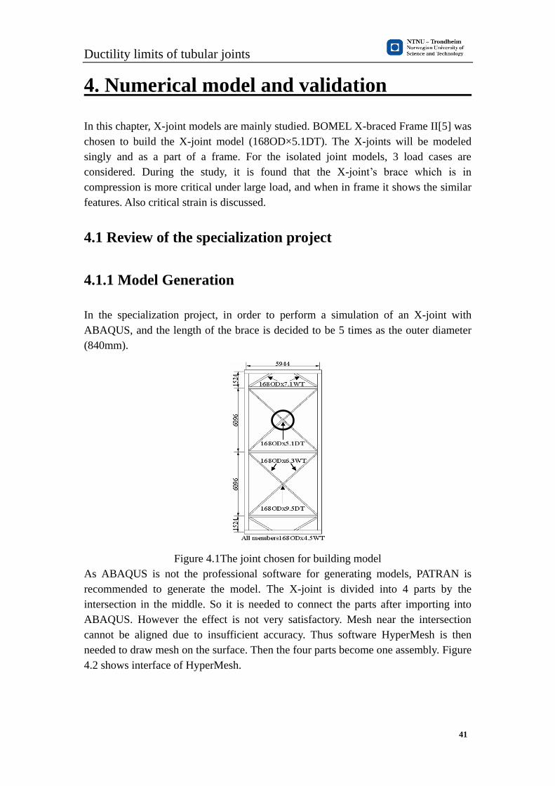
Ductility limits of tubular joints
41
4. Numerical model and validation
In this chapter, X-joint models are mainly studied. BOMEL X-braced Frame II[5] was
chosen to build the X-joint model (168OD×5.1DT). The X-joints will be modeled
singly and as a part of a frame. For the isolated joint models, 3 load cases are
considered. During the study, it is found that the X-joint’s brace which is in
compression is more critical under large load, and when in frame it shows the similar
features. Also critical strain is discussed.
4.1 Review of the specialization project
4.1.1 Model Generation
In the specialization project, in order to perform a simulation of an X-joint with
ABAQUS, and the length of the brace is decided to be 5 times as the outer diameter
(840mm).
Figure 4.1The joint chosen for building model
As ABAQUS is not the professional software for generating models, PATRAN is
recommended to generate the model. The X-joint is divided into 4 parts by the
intersection in the middle. So it is needed to connect the parts after importing into
ABAQUS. However the effect is not very satisfactory. Mesh near the intersection
cannot be aligned due to insufficient accuracy. Thus software HyperMesh is then
needed to draw mesh on the surface. Then the four parts become one assembly. Figure
4.2 shows interface of HyperMesh.

Ductility limits of tubular joints
42
Figure 4.2 Auto-meshing the joint by using HyperMesh
After Hypermesh, the four separate parts become together as one part, the intersection
places are connected well to each other. Now it can be imported to ABAQUS for
doing the analysis.
Figure 4.3 Mesh and model in ABAQUS
Three load cases are to be used which is shown in Figure 4.4
N1 is compression force and N2 is tension force.
Load case 1: N2=0,
Load case 2: N2=N1
Load case 3: N2=0.5N1

Ductility limits of tubular joints
43
Figure 4.4 Load distributions on the joint
4.1.2 Analysis results
First axial resistance defined by Norsok-004 is calculated by using the formulations
mentioned in Chapter 2.
The above geometry parameters of the model:
β=1, γ=168
10.2=16.47, τ=1, α=
2L
D=10, fy=345N/mm
2
NRd=fyT
2
γMsinθ
QuQf=345×5.12
1.15×1QuQf
Qβ=
0.3
β(1-0.833β)=0.3
0.167=1.7964
Qu=(2.8+14β)Q
β=16.8×1.7964=30.17952
A=C1 (σa,Sd
fy)
2
+C2 (σmy,Sd2 +σmz,Sd
2
1.62fy2
)=20× (200
345)2
+22×(1502×2
1.62×3452)=11.854
Qf=1.0
N1 N1
N2
N2

Ductility limits of tubular joints
44
NRd=fyT
2
γMsinθ
QuQf=345×5.12
1.0×1QuQf=270814.4N
Estimated values are made for σmy,Sd and σmz,Sd.
The history output is set to displacement of the reference point and Load proportional
factor. The displacement-load curves are plotted after the calculation. The
force-deformation behaviour of the joint in different cases is shown in Fig. 4.5.
Figure 4.5 Displacement-LPF curves
From Figure 4.5 we can see that the curves’ tendencies are similar: at the first stage
displacement changes little while the LPF rises sharply, and then the slope of the
curves become smaller. At the end the slope becomes near to zero, i.e. the
displacement is increasing while the LPF doesn’t change much, which corresponds to
the plastic deformation. Also the figure indicates the comparison with resistance
calculated by Norsok004. We can see that the Norsork004 resistance is much smaller
than the magnitude of the inflection point of the curves, which indicates that the code
calculated values are conservative. More reasonable measures may be recommended.
The three curves are compared also. From Figure 4.5 we can see the capacity of the
joints is more sufficient when no axial tension load is applied on them. When axial
tension load is added to the joints, the LPF is smaller at the same displacement than
the one without tension load. The larger the tension load is, the less sufficient capacity
the joints show.
N2=0N1
N2=0.5N1
N2=N1
Resistance calculated by
norsok-004

Ductility limits of tubular joints
45
However, the curves obtained are not so satisfactory because the curve is always on
the rise without descent stage, which is inconsistent with the actual reality.
4.2 Work in master thesis
In the master thesis project, a lot more work has been done for this joint model. And
the curves obtained in specialization project are proved to be not so correct, though
deformation type is similar with the experimental test. The major reason of this is due
to non-linear effects not taken into account.
4.2.1 The application of Riks method
The line-perturbation is the eigenvalue analysis of buckling. It is a linear analysis,
while non-linear buckling analysis is to be performed. In order to do so, initial
imperfection is to be imported.
ABAQUS has three methods to identify initial imperfection: taking a linear
combination of the branch buckling model, taking the results based on static analysis,
specifying directly. The first method is normally used, and the procedures are as
follows:
1. Write the eigenmodes in the default global system to the results file as nodal data
2. Add the eigenmodes to the perfect geometry as the initial imperfection, and the
associated scale factor is largest in the 1st modeshape. The scale factor is usually taken
as the multiple of the geometry parameters, for example, 0.1 times of the shell
thickness, etc.
3. Analyze by using the riks method.
Defining an imperfection based on eigenmode data
Input File Usage:
*IMPERFECTION, FILE=results file, STEP=step, NSET=name
Defining an imperfection based on static analysis data
In order to use the eigenvalue file, the model keywords of the buckle is to be
modified.
*node file,
*u
Add these two sentences to the keywords. The location is shown in figure below.

Ductility limits of tubular joints
46
4.2.2 Model generation
First, the material is optimized by adding hardening area in order to make it closer to
the reality.
The yield criterion states that yielding begins when stress reaches yield stress, in
practice usually taken as the tensile yield strength. Subsequent plastic deformation
may alter the stress needed to produce renewed or continued yielding
Yield Stress Plastic Strain
1 355 0
2 410 0.05
3 450 0.1
4 480 0.15
Figure 4.6 Material stress and strain relation curve
As required in the master thesis task, analysis is to be performed with single joints and
0
100
200
300
400
500
600
-0.02 0 0.02 0.04 0.06 0.08 0.1 0.12 0.14 0.16
Str
ess/
MP
a
Strain

Ductility limits of tubular joints
47
joints as a part of a frame system plane frame system, so a model of single joint as a
part of a frame system is built as shown in Figure 4.7. And a push-over analysis is to
be performed.
Figure 4.7 Single joint as a part of a frame system
The dimension of the frame are shown in Figure 4.8
Figure 4.8 Dimension

Ductility limits of tubular joints
48
The constraint type of coupling is used as the interaction between the frame edges and
the joint (See Figure 4.9).
Figure 4.9 Interaction used between frame and joint
In reality, a through member is usually used when a joint is built by the same method
mentioned, i.e. the joint consists of a through member and two separate braces welded
to the through member, which is shown in Figure 4.10.
Figure 4.10 new joint model with a through member
Similarly, a model of this single joint as a part of a frame system is built with the
same dimension.
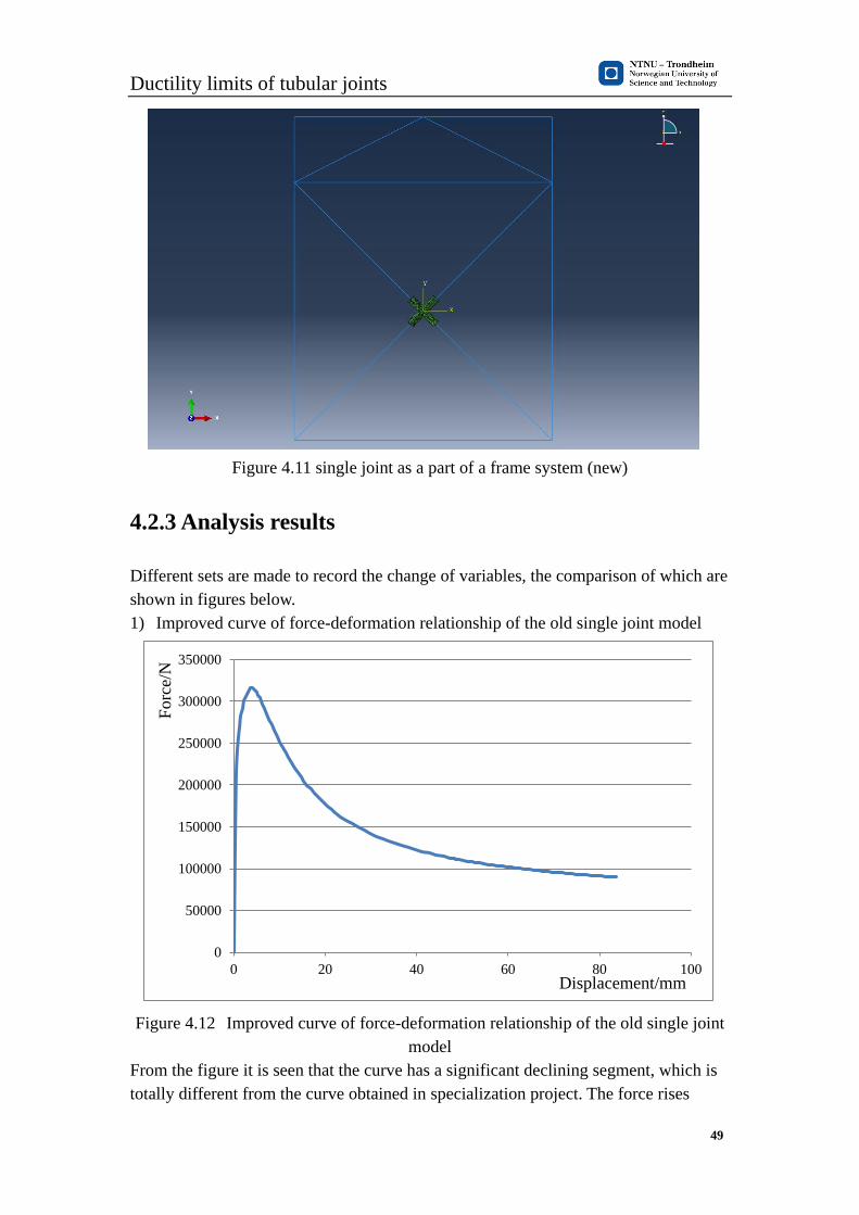
Ductility limits of tubular joints
49
Figure 4.11 single joint as a part of a frame system (new)
4.2.3 Analysis results
Different sets are made to record the change of variables, the comparison of which are
shown in figures below.
1) Improved curve of force-deformation relationship of the old single joint model
Figure 4.12 Improved curve of force-deformation relationship of the old single joint
model
From the figure it is seen that the curve has a significant declining segment, which is
totally different from the curve obtained in specialization project. The force rises
0
50000
100000
150000
200000
250000
300000
350000
0 20 40 60 80 100
Forc
e/N
Displacement/mm

Ductility limits of tubular joints
50
sharply at the first stage until it reaches the critical load, after which it declined
rapidly with the increase of the displacement. The difference can be explained by
whether non-linear effects are taken into account or not, which, in ABAQUS, is
reflected by choosing nlgeom or not (geometry in non-linear).
The deformation and plot of stresses of the joint in different stages are shown in
Figure 4.13.
Figure 4.13 the deformation and plot of stresses of the joint in different stages
As shown in the figure 4.13, the joint has a very obvious buckling, as the compression
brace warps and compresses the tension braces.
2) The curve of force-deformation relationship of the new single joint model
Figure 4.14 the curve of force-deformation relationship of the new single joint model
The curve of force-deformation relationship of the new single joint model shows the
same trend as the old single one, also the deformation and plot of stresses of the joint
in different stages.
Figure 4.15 the deformation and plot of stresses of the joint in different stages
0
50000
100000
150000
200000
250000
300000
350000
400000
0 20 40 60 80 100 120 140
Forc
e/N
Displacement/mm

Ductility limits of tubular joints
51
3) Comparison of the two curves of the two different models.
Figure 4.16 Comparison of the force-displacement relation curve of the old and new
joint model
From the figure it is seen that the new joint model has a larger critical load than the
old one, which proves that the through member makes a contribution to the capacity
of the joints.
4) The old single joint as a part of a frame system
The LPF and global displacement relation curve is shown in Figure 4.17
Figure 4.17 the LPF and global displacement relation
From the Figure 4.17 it is seen that in the curve at the first stage displacement changes
little while the LPF rises sharply, and then the slope of the curves become smaller.
This is similar with the result of the specialization project. But in fact they are
different, for which non-linear effect has been taken into account, and the result can
be explained by the figures below.
0
50000
100000
150000
200000
250000
300000
350000
400000
0 20 40 60 80 100 120 140
old joint model
new joint model
0
0.1
0.2
0.3
0.4
0.5
0.6
0.7
0 100 200 300 400
Forc
e/N
Displacement/mm
LP
F
Displacement/mm
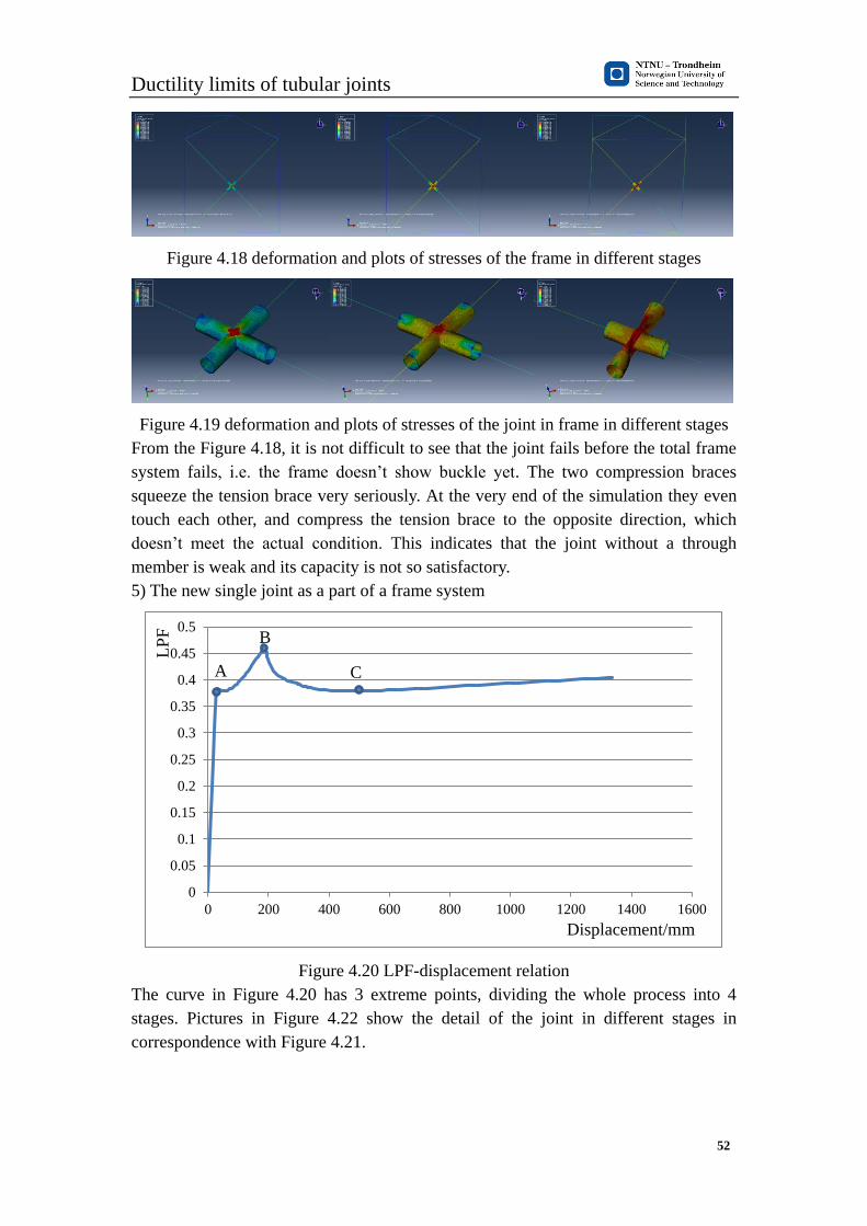
Ductility limits of tubular joints
52
Figure 4.18 deformation and plots of stresses of the frame in different stages
Figure 4.19 deformation and plots of stresses of the joint in frame in different stages
From the Figure 4.18, it is not difficult to see that the joint fails before the total frame
system fails, i.e. the frame doesn’t show buckle yet. The two compression braces
squeeze the tension brace very seriously. At the very end of the simulation they even
touch each other, and compress the tension brace to the opposite direction, which
doesn’t meet the actual condition. This indicates that the joint without a through
member is weak and its capacity is not so satisfactory.
5) The new single joint as a part of a frame system
Figure 4.20 LPF-displacement relation
The curve in Figure 4.20 has 3 extreme points, dividing the whole process into 4
stages. Pictures in Figure 4.22 show the detail of the joint in different stages in
correspondence with Figure 4.21.
0
0.05
0.1
0.15
0.2
0.25
0.3
0.35
0.4
0.45
0.5
0 200 400 600 800 1000 1200 1400 1600
A
B
C
LP
F
Displacement/mm

Ductility limits of tubular joints
53
a.1st stage b.2
nd stage
c. 3
rd stage d. 4
th stage
Figure 4.21 deformation and plots of stresses of the frame in different stages
In Figure 4.21(a), the whole frame starts to deform, and yielding occurs in the joint,
which corresponds to point A in Figure 4.20.
In Figure 4.21(b), the frame has tilted to a certain extent, and the lower brace in
compression starts to buckle and can take no more load corresponding to point B in
Figure 4.20.
In figure 4.21(c), the frame system starts to regain strength because the rest of braces
take the load instead, which corresponds to point C.
Figure 4.21(d) shows the end of the simulation, and the frame system has undergone a
drastic shift compared to the initial position.
a. 1st stage b. 2
nd stage

Ductility limits of tubular joints
54
c. 3rd
stage d. 4th
stage
Figure 4.22 the detail of the joint in frame in different stages in correspondence with
Figure 4.20
Figure 4.23 the relationship of the axial force of the upper compression brace and the
length of the compression joint brace
Figure 4.23 shows the relationship of the axial force of the upper compression brace
and the length of the compression joint brace (rotate deformation of the joint
neglected). Similar with the force-displacement curve of new single joint as a part of a
frame system, it has also 3 extreme points (Yielding occurs at Point A, Buckle starts at
Point B, and the brace starts regaining strength at Point C).
6) Strain development of the joint
In order to study the strain of the joint, 3 sets are created to observe the strain
development of different position of the joint, the positions of which are shown in Fig.
4.24.
0
100000
200000
300000
400000
500000
600000
670720770820
Forc
e/N
Length/mm
A B
C
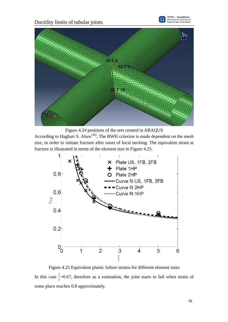
Ductility limits of tubular joints
55
Figure 4.24 positions of the sets created in ABAQUS
According to Hagbart S. Alsos[36]
, The BWH criterion is made dependent on the mesh
size, in order to imitate fracture after onset of local necking. The equivalent strain at
fracture is illustrated in terms of the element size in Figure 4.25.
Figure 4.25 Equivalent plastic failure strains for different element sizes
In this case l
t=0.67, therefore as a estimation, the joint starts to fail when strain of
some place reaches 0.8 approximately.
SET 8
SET 9
SET 10
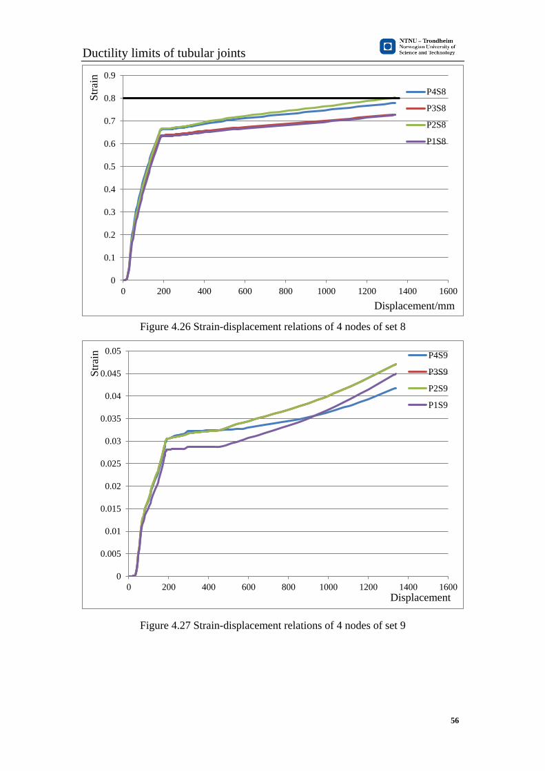
Ductility limits of tubular joints
56
Figure 4.26 Strain-displacement relations of 4 nodes of set 8
Figure 4.27 Strain-displacement relations of 4 nodes of set 9
0
0.1
0.2
0.3
0.4
0.5
0.6
0.7
0.8
0.9
0 200 400 600 800 1000 1200 1400 1600
P4S8
P3S8
P2S8
P1S8
0
0.005
0.01
0.015
0.02
0.025
0.03
0.035
0.04
0.045
0.05
0 200 400 600 800 1000 1200 1400 1600
P4S9
P3S9
P2S9
P1S9
Displacement/mm
Str
ain
Displacement
Str
ain
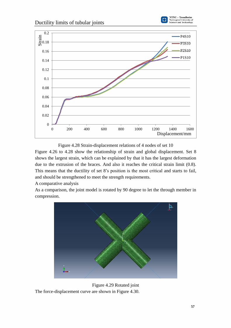
Ductility limits of tubular joints
57
Figure 4.28 Strain-displacement relations of 4 nodes of set 10
Figure 4.26 to 4.28 show the relationship of strain and global displacement. Set 8
shows the largest strain, which can be explained by that it has the largest deformation
due to the extrusion of the braces. And also it reaches the critical strain limit (0.8).
This means that the ductility of set 8’s position is the most critical and starts to fail,
and should be strengthened to meet the strength requirements.
A comparative analysis
As a comparison, the joint model is rotated by 90 degree to let the through member in
compression.
Figure 4.29 Rotated joint
The force-displacement curve are shown in Figure 4.30.
0
0.02
0.04
0.06
0.08
0.1
0.12
0.14
0.16
0.18
0.2
0 200 400 600 800 1000 1200 1400 1600
P4S10
P3S10
P2S10
P1S10
Str
ain
Displacement/mm

Ductility limits of tubular joints
58
Figure 4.30 Comparison of the force-displacement curves
From the figure it is easy to see that if through member is made in compression, the
critical load when yielding occurs is larger than when it is made in tension. And the
displacement of the frame is much smaller than the previous one. This is because the
buckling of the braces is out-of-plane buckling, while the previous one is in-plane
buckling. That means that this kind of frame is more stable than previous one.
Figure 4.31 out-of-plane buckling
0
200000
400000
600000
800000
1000000
1200000
1400000
0 200 400 600 800 1000 1200 1400 1600
through member in
tension
through member in
compressionForc
e/N
Displacement/mm
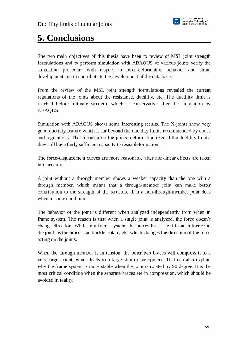
Ductility limits of tubular joints
59
5. Conclusions
The two main objectives of this thesis have been to review of MSL joint strength
formulations and to perform simulation with ABAQUS of various joints verify the
simulation procedure with respect to force-deformation behavior and strain
development and to contribute to the development of the data basis.
From the review of the MSL joint strength formulations revealed the current
regulations of the joints about the resistance, ductility, etc. The ductility limit is
reached before ultimate strength, which is conservative after the simulation by
ABAQUS.
Simulation with ABAQUS shows some interesting results. The X-joints show very
good ductility feature which is far beyond the ductility limits recommended by codes
and regulations. That means after the joints’ deformation exceed the ductility limits,
they still have fairly sufficient capacity to resist deformation.
The force-displacement curves are more reasonable after non-linear effects are taken
into account.
A joint without a through member shows a weaker capacity than the one with a
through member, which means that a through-member joint can make better
contribution to the strength of the structure than a non-through-member joint does
when in same condition.
The behavior of the joint is different when analyzed independently from when in
frame system. The reason is that when a single joint is analyzed, the force doesn’t
change direction. While in a frame system, the braces has a significant influence to
the joint, as the braces can buckle, rotate, etc. which changes the direction of the force
acting on the joints.
When the through member is in tension, the other two braces will compress it to a
very large extent, which leads to a large strain development. That can also explain
why the frame system is more stable when the joint is rotated by 90 degree. It is the
most critical condition when the separate braces are in compression, which should be
avoided in reality.

Ductility limits of tubular joints
60

Ductility limits of tubular joints
61
6. Recommendations for further work
Far from enough verification and validation is done. Also more variables need to be
controlled and analyzed.
In this paper, only X-joints are analyzed, and the X-joints are the simplest ones, i.e.
the two braces are of same length, diameter and wall thickness. In the future, other
types of joints such as T joints or K joints may also be analyzed and compared. Also
different brace geometry can be applied to see the effect they have to the joints
capacity.
Due to limited time, analysis of the frame with usfos nonlinear joint has not been
finished. So it is necessary to do it in the future.
In addition, the conservativeness concluded in this paper shows that current codes and
regulations may be recommended to modify to reduce the conservativeness.

Ductility limits of tubular joints
62

Ductility limits of tubular joints
63
Reference
[1] NORSOK STANDARD, N-004 Rev. 2, October 2004, Design of steel structures.
[2] OMAE2011, Proceedings of the ASME201130th International Conference on
Ocean, Offshore and Arctic Engineering, June 19-24, 2011, OMAE2011-49874,
Safety Format and Acceptance Criteria for Analysis of Marine Structures Using
Non-linear Methods.
[3]-[7] Jørgen Amdahl, FRAME STUDY, Chapter 8.
[8] Van der Vegte, G.J. (1995). The static strength of uniplanar and multiplanar
tubular T- and X-joints, PhD thesis, Delft University of Technology, The Netherlands.
[9] USFOS Manual, USFOS Joint Capacity Theory, Description of use Verification.
[10]Hagbart S.Alsos (2007) Analytical and numerical analysis of sheet metal
instability using a stress based criterion
[11] Keeler, S.P., Backhofen,W.A., 1964. Plastic instability and fracture in sheet
stretched over rigid punches. ASM Transactions Quarterly 56,
25–48.
[12] Goodwin, G.M., 1968. Application of strain analysis to sheet metal forming in
the press shop. In: SAE paper 680093.
[13][15][24]Ghosh, A.K., Laukonis, J.V., 1976. The influence of strain path changes
on the formability of sheet steel. In: 9th Biennial Congress of the IDDRG, Sheet
Metal Forming and Energy Conservation. ASM Publication.
[14][17][25] Graf, A.F., Hosford, W.F., 1993. Calculations of forming limit diagrams
for changing strain paths. Metal Transactions A 24, 2497–2501.
[16] Barata da Rocha, A., Barlat, F., Jalinier, J.M., 1985. Prediction of the forming
limit diagram of anisotropic sheets in linear and non-linear loading. Materials Science
and Engineering 68, 151–164.
[18] Arrieux, R., Bedrin, C., Boivin, M., 1982. Determination of an intrinsic forming
limit stress diagram for isotropic metal sheets. In:Proceedings of the 12th Biennial
Congress IDDRG, pp. 61–71.
[19][26] Stoughton, T.B., 2001. Stress-based forming limits in sheet metal forming.
Journal of Engineering Materials and Science 123, 417–422.
[20][27][29]Stoughton, T.B., Zhu, X., 2004. Review of theoretical models of the
strain-based fld and their relevance to the stress-based fld. International Journal of
Plasticity 20, 1463–1486.
[21] Wu, P.D., Graf, MacEwen, S.R., Lloyd, D.J., Jain, M., Neale, K.W., 2005. On
forming limit stress diagram analysis. International Journal of Solids and Structures
42, 2225–2241.
[22] Hallquist, J., 2007a. Ls-dyna keyword users manual—ls971. Technical report,
Livemore Software.
Hallquist, J., 2007b. Ls-dyna theory manual— ls971. Technical report, Livemore
Software.

Ductility limits of tubular joints
64
[23] Tornqvist, R., 2003. Design of crashworthy ship structures. Ph.D. thesis, DTU.
[28] Hill, R., 1952. On discontinuous plastic states with special reference to localized
necking in thin sheets. Journal of the Mechanics and Physics of Solids 1, 19–30.
[30] Marciniak, Z., Kuczynski, K., 1967. Limit strains in processes of stretch forming
sheet metal. Journal of Mechanical Sciences 9, 609–620.
[31] [32] Bressan, J.D., Williams, J.A., 1983. The use of a shear instability criterion to
predict local necking in sheet metal deformation. International Journal of Mechanical
Science 25, 155–168.
[33] Brunet, M., Clerc, P., 2007. Two prediction methods for ductile sheet metal
failure. In: ESAFORM Conference on Material Forming.
[34] TMR4305 Chapter 12 - Nonlinear Analysis
[35] ABAQUS Users’ Manual
[36] Hagbart S. Alsos , Ship Grounding,Analysis of Ductile Fracture, Bottom
Damage and Hull Girder Response, PHD Thesis, NTNU On the resistance to
penetration of stiffened plates, Part II – Numerical analysis