Ab InitioAb Initio Molecular Dynamics with a Molecular Dynamics with a

Continuum Solvation ModelContinuum Solvation Model

Ab InitioAb Initio Molecular Dynamics with a Molecular Dynamics with a

Continuum Solvation ModelContinuum Solvation Model

Hans Martin Senn, Tom Ziegler

University of Calgary

CSC 2002 Conference, Vancouver, BC, 2 June 2002

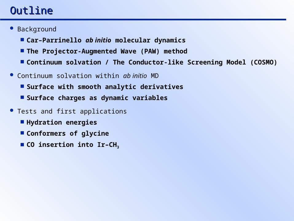
OutlineOutline

Background Car–Parrinello ab initio molecular dynamics The Projector-Augmented Wave (PAW) method Continuum solvation / The Conductor-like Screening Model (COSMO)

Continuum solvation within ab initio MD Surface with smooth analytic derivatives Surface charges as dynamic variables

Tests and first applications Hydration energies Conformers of glycine

CO insertion into Ir–CH3

Ab initio molecular dynamics

Ab initio molecular dynamicsForces on nuclei derived from

instantaneous electronic structure

Ab initio molecular dynamicsForces on nuclei derived from

instantaneous electronic structure

Ab InitioAb Initio Molecular Dynamics Molecular DynamicsR. Car, M. Parrinello, Phys. Rev. Lett. 1985, 55,

2471Nuclei

Classical mechanics

ElectronsDensity-functional

theory

€

MJ ˙ ̇ R J = −∂E {RI},{c i}[ ]

∂RJ

mc ˙ ̇ c j = −dE {RI},{c i}[ ]

d c j+ c i L iji∑

Car–Parrinello scheme for ab initio MD Fictitious dynamics of the wavefunctions Simultaneous treatment of atomic and electronic structure

Friction dynamics for minimizations

€

+ =T −V = 12

M J˙ R J

2J∑

nuclear kin. energy1 2 4 3 4

+ mc˙ c i

˙ c ii∑fictitious kin. energyof the wavefunctions

1 2 4 4 3 4 4 − E {RI },{c i}[ ]

DFT total energy1 2 4 4 3 4 4

+ c i c j −dij( )L jii, j∑orthonormality constraint

1 2 4 4 4 4 3 4 4 4 4

Basis set: Augmented plane waves Spatial decomposition of the wavefunction according to its shape

Smooth plane-wave expansion far from nuclei

Rapidly oscillating augmentation functions around the nuclei

Integrations for total energy and matrix elements decompose accordingly Smooth parts in Fourier representation

One-centre parts on radial grids in spherical harmonics expansions

All-electron method Frozen-core approximation

c = ˜ c + f k ˜ p k ˜ c −

k∑ ˜ f k ˜ p k ˜ c k∑

The Projector-Augmented Wave (PAW) MethodThe Projector-Augmented Wave (PAW) MethodP.E. Blöchl, Phys. Rev. B 1994, 50,

17953

€

˜ c (r) = c (G)eiG rG∑ Plane-wave expansion

f k (r) = x k Yl ,m Numerical, atomic-orbital-like functions

˜ f k (r) Smoothened atomic orbitals

˜ p k (r) Projector functions

Continuum Solvation ModelsContinuum Solvation Models

Implicit electrostatic solvation “Solvent” = homogeneous, isotropic dielectric medium

Fully characterized by relative permittivity (r)

Electrostatic interactions

1. Solute polarizes the dielectric ( reaction field) Epol > 0

2. Solute charge density interacts with polarized medium Eint < 0

3. Solute electronic and atomic structure adapt (“back-polarization”) ∆Een > 0

4. Repeat to self-consistency!

€

Gdiel = Eint + Epol = 12 Eint

€

Gdiel = Eint + Epol = 12 Eint

Electrostatic free energy For a linear dielectric:

The Solvation EnergyThe Solvation Energy

Non-electrostatic contributions Cavity formation Dispersion and exchange-repulsion Approximately proportional to cavity surface area

€

Gsol = Eensol +Gdiel + Gnp

ΔsolvG = Gsol − Eeng = Gdiel +Gnp + DEen

€

Gsol = Eensol +Gdiel + Gnp

ΔsolvG = Gsol − Eeng = Gdiel +Gnp + DEen

€

Gnp = b +gA

€

Gnp = b +gA

Free energy of solvation

Neglect changes in thermal motion upon solvation

The Conductor-Like Screening Model (COSMO)The Conductor-Like Screening Model (COSMO)

Main approximations in COSMO

1. Dielectric with infinite permittivity (r ∞)

No volume polarization; polarization expressed as surface charge density only

Vanishing potential at the cavity boundary

€

Gdiel∞ s[ ] = d3r d2s

r (r)s (s)r − sS∫V∫ +

12

d2s d2 ′ s s (s)s ( ′ s )

s − ′ s S∫S∫

€

Gdiel∞ s[ ] = d3r d2s

r (r)s (s)r − sS∫V∫ +

12

d2s d2 ′ s s (s)s ( ′ s )

s − ′ s S∫S∫

€

f ∞(s) =dGdiel

∞

dss

= d3rr (r)r − sV∫ + d2 ′ s

s ( ′ s )s − ′ s S∫ = 0

€

f ∞(s) =dGdiel

∞

dss

= d3rr (r)r − sV∫ + d2 ′ s

s ( ′ s )s − ′ s S∫ = 0

€

GdielCOSMO = fGdiel

∞ s[ ]

s (s) = fs (s)

€

GdielCOSMO = fGdiel

∞ s[ ]

s (s) = fs (s)

€

GdielCOSMO {qi}( ) = qi d3r

r (r)r − siV∫

i∑ +

12 f

qiq j

si − s ji, j( j≠i )

∑ +1.07 4p

2 fqi

2

aii∑

€

GdielCOSMO {qi}( ) = qi d3r

r (r)r − siV∫

i∑ +

12 f

qiq j

si − s ji, j( j≠i )

∑ +1.07 4p

2 fqi

2

aii∑

2. Recover true dielectric behaviour by scaling Derived for rigid multipoles in spherical cavity

f = f(r) = (r – 1) / (r + x) [x = 0, 1/2 for monopole, dipole]

3. Discretize cavity surface and surface charge Surface segments carrying point charges qi

Energy expression is variational in qi

Surface Charges as Dynamic VariablesSurface Charges as Dynamic Variables Extended Lagrangean including solvation

Equations of motion for charges

€

+ =+ CP + mq ˙ q i2

i∑ − Gdiel

COSMO {RJ},{q j}( ) −Gnp {RJ}( )

€

+ =+ CP + mq ˙ q i2

i∑ − Gdiel

COSMO {RJ},{q j}( ) −Gnp {RJ}( )

€

mq˙ ̇ q i =∂ +∂qi

−mq ˙ q zq

€

mq˙ ̇ q i =∂ +∂qi

−mq ˙ q zq

Additional forces acting on the nuclei Surface segments and charges implicitly depend on atomic positions via the surface

construction

Forces obtained as analytic derivatives

Energy-conserving dynamics requires smooth derivatives Segments/charges must not vanish or be created during the simulation

Each segment/charge must be unambiguously assigned to an atom

Conventional schemes for building the cavity are not compatible with this!

Surface ConstructionSurface Construction

A surface construction compatible with AIMD

1. Surface = union of atomic spheres

2. Each sphere is triangulated

3. All segments and charges are retained

Each segment/charge moves rigidly along with its atom

€

GdielCOSMO = qiQ i d3r

r (r)r − siV∫

i∑ +

12 f

qiQ iq jQ j

si − sji, j( j≠i)

∑ +1.07 p

fqi

2Q i2

aii∑

4. A switching function effectively removes charges lying within another

sphere from the energy expression

i = 1 if the charge is exposed on the molecular surface

i = 0 if the charge is buried

Smooth transition between “on” and “off”

Total switching function

Charge is smoothly switched off if it lies within any one of the other spheres

Switching FunctionsSwitching Functions

Building the switching function Rectangular pulse

Centred at d0 = Rsolv – c

Vanishes smoothly at d0

€

h(d, d0) =1 − exp − d −d0( )

2n ⎡

⎣ ⎢ ⎢

⎤

⎦ ⎥ ⎥, n∈N

€

h(d,d0) =1 − exp − d −d0( )

2n ⎡

⎣ ⎢ ⎢

⎤

⎦ ⎥ ⎥, n∈N

n = 1n = 10n = 24

d0 Rsolv

€

uJ,i =h RJ − si ,dJ

0( ) for RJ − si > dJ

0

0 for RJ − si ≤ dJ0

⎧ ⎨ ⎪

⎩ ⎪

€

uJ,i =h RJ − si ,dJ

0( ) for RJ − si > dJ

0

0 for RJ − si ≤ dJ0

⎧ ⎨ ⎪

⎩ ⎪

d

€

Qi = uJ ,iJ

(J ≠I(i))

∏

€

Qi = uJ ,iJ

(J ≠I(i))

∏

Atomic switching function

RAsolv

RBsolv

Rounding the Edges…Rounding the Edges…

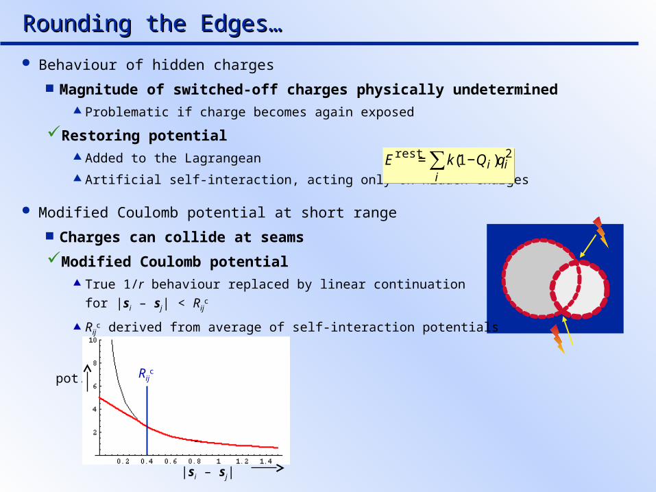
Behaviour of hidden charges Magnitude of switched-off charges physically undetermined

Problematic if charge becomes again exposed

Restoring potential Added to the Lagrangean

Artificial self-interaction, acting only on hidden charges

€

Erest = k(1−Qi )qi2

i∑

€

Erest = k(1−Qi )qi2

i∑

pot.

|si – sj|

Rijc

Modified Coulomb potential at short range Charges can collide at seams

Modified Coulomb potential True 1/r behaviour replaced by linear continuation

for |si – sj| < Rijc

Rijc derived from average of self-interaction potentials

Representation of the Solute DensityRepresentation of the Solute Density

Decoupling of periodic images Plane-wave-based methods always create periodic images

Artificial in molecular calculations

Electrostatic decoupling scheme in PAW Model density

Superposition of atom-centred Gaussians

Coefficients determined by fit to true density

Reproduces long-range behaviour

Surface charges couple to model density Not instrumental Computationally convenient

3–5 Gaussians per atom

Fitting procedure relays forces acting on the wave functions due to the charges

€

ˆ r (r) = QI ,mgI ,m (r)I ,m∑

€

ˆ r (r) = QI ,mgI ,m (r)I ,m∑

€

Es–m =qiQ iQI ,m

RI − sierf RI − si rI ,m

c[ ]

i,I ,m∑

€

Es–m =qiQ iQI ,m

RI − sierf RI − si rI ,m

c[ ]

i,I ,m∑

Parameterization Free energies of hydration

Parameters: Solvation radii RIsolv, non-polar parameters ,

Fit set: Neutral organic molecules containing C, H, O, N

Mean unsigned error (MUE) over whole set: 4.1 kJ/mol On par with similar DFT/COSMO results

5.2 kJ/mol4.2 kJ/molMUE: 3.2 kJ/mol

Parameterization and ValidationParameterization and Validation

CH4

H

H

OH

OH

OH

O

O

H

O

O

OH

O

O

OH

OH

OH O

H

NH3

H2N

NH N

N

NH2

NO2

NH

O

NH2

ONH

O

NH

O

Conformers of GlycineConformers of Glycine

H-bonding patterns

Relative stabilities (kJ/mol)

Hydration energies (kJ/mol)

A

BC Z

Gas phase Aqueous phaseMethod C A B Method Z A BPAW 0 4.1 9.6 PAW/COSMO 0 49 55Other pure DFT 0 1.1…4.6 6.8 Other pure DFT 0 36…39Hybrid DFT 0 –1.6…–1.1 4.7…5.6 Hybrid DFT 0 13Expt. 0 –5.9 Expt. 30…32

Method ∆hydGA(g) → A(a )q A(g) → Z(a )q

PAW/COSMO –57 –105Ot her pureDFT –54 –91Hybri d DFT –49…–42 –61…–57Expt. –80

Zwitterion in solution Most stable conformer

Not present in the gas phase

Energy ConservationEnergy Conservation

Conservation of total energy Glycine without and with continuum solvation

∆t = 7 a.u., T ≈ 300 K (no thermostats, no friction)

Drift in total energy: solvation off +2.78  5 Eh/ps per atom

solvation on 1.43  5 Eh/ps per atom

Energy is conserved

A First ApplicationA First Application

Carbonylation of methanol “Monsanto” / ”Cativa” acetic-acid process

M = Rh, Ir

Via [MI3(CH3)(CO)2]– [MI3(COCH3)(CO)]–

AIMD simulation of CO insertion step Solvent: iodomethane; T = 300 K

Slow-growth thermodynamic integration along d(CMe–CCO)

∆A‡ = 111  (128) kJ/mol∆E‡ = 126  (155) kJ/mol; ∆S‡ = 60  (91) J/(K mol)

Dissociation of I– trans to incipient acyl! Only in solution at finite temperature

Enthalpy of Ir–I bond traded for entropy of free (solvated) I–

MeOHCO

MeCOOHcat. [MI2(CO)2]

–, HI, H2OMeOH

COMeCOOH

cat. [MI2(CO)2]–, HI, H2O

RC

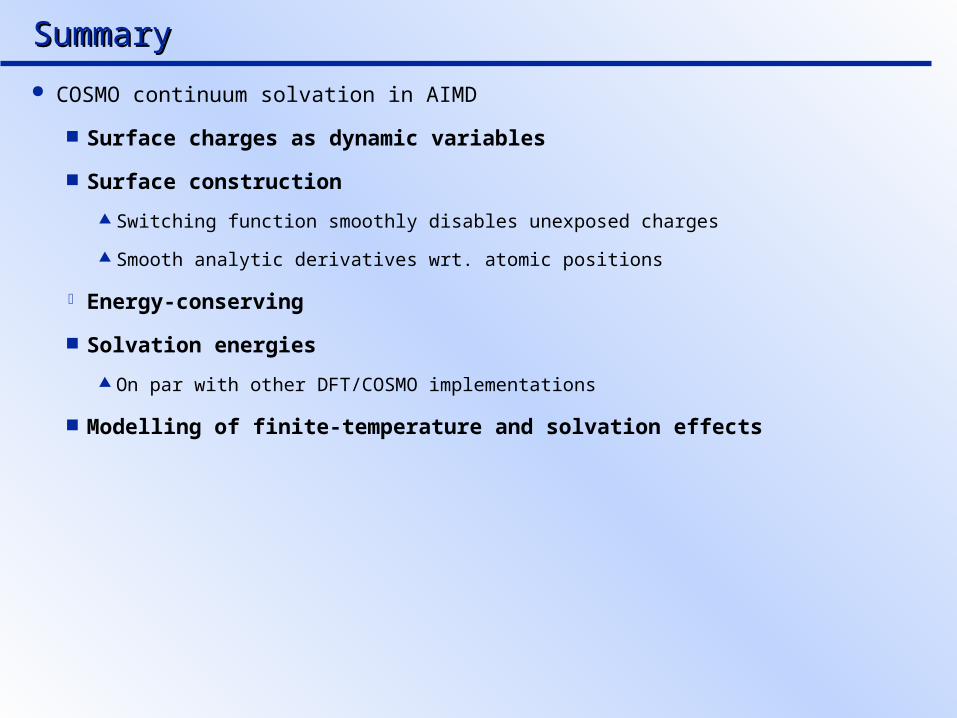
SummarySummary

COSMO continuum solvation in AIMD

Surface charges as dynamic variables

Surface construction

Switching function smoothly disables unexposed charges

Smooth analytic derivatives wrt. atomic positions

Energy-conserving

Solvation energies

On par with other DFT/COSMO implementations

Modelling of finite-temperature and solvation effects

AcknowledgmentsAcknowledgments

Peter E. Blöchl,Institute of Theoretical Physics, Clausthal University of Technology, Germany

Peter M. Margl,Corporate R&D Computing, Modeling and Information Sciences, Dow

Rochus Schmid,Institute of Inorganic Chemistry, Munich University of Technology, Germany

$ Swiss National Science Foundation

$ NSERC

$ Petroleum Research Fund