Aalborg Universitet Feature Based Control of Compact Disc ...
199
Aalborg Universitet Feature Based Control of Compact Disc Players Odgaard, Peter Fogh Publication date: 2004 Document Version Også kaldet Forlagets PDF Link to publication from Aalborg University Citation for published version (APA): Odgaard, P. F. (2004). Feature Based Control of Compact Disc Players. Aalborg Universitet. General rights Copyright and moral rights for the publications made accessible in the public portal are retained by the authors and/or other copyright owners and it is a condition of accessing publications that users recognise and abide by the legal requirements associated with these rights. ? Users may download and print one copy of any publication from the public portal for the purpose of private study or research. ? You may not further distribute the material or use it for any profit-making activity or commercial gain ? You may freely distribute the URL identifying the publication in the public portal ? Take down policy If you believe that this document breaches copyright please contact us at [email protected] providing details, and we will remove access to the work immediately and investigate your claim. Downloaded from vbn.aau.dk on: December 27, 2020
Transcript of Aalborg Universitet Feature Based Control of Compact Disc ...

Aalborg Universitet
Feature Based Control of Compact Disc Players
Odgaard, Peter Fogh
Publication date:2004
Document VersionOgså kaldet Forlagets PDF
Link to publication from Aalborg University
Citation for published version (APA):Odgaard, P. F. (2004). Feature Based Control of Compact Disc Players. Aalborg Universitet.
General rightsCopyright and moral rights for the publications made accessible in the public portal are retained by the authors and/or other copyright ownersand it is a condition of accessing publications that users recognise and abide by the legal requirements associated with these rights.
? Users may download and print one copy of any publication from the public portal for the purpose of private study or research. ? You may not further distribute the material or use it for any profit-making activity or commercial gain ? You may freely distribute the URL identifying the publication in the public portal ?
Take down policyIf you believe that this document breaches copyright please contact us at [email protected] providing details, and we will remove access tothe work immediately and investigate your claim.
Downloaded from vbn.aau.dk on: December 27, 2020
Feature Based Control of CompactDisc Players
Ph.D. Thesis
by
Peter Fogh Odgaard
Department of Control EngineeringAalborg University
Fredrik Bajers Vej 7C, DK-9220 Aalborg Ø, Denmark.

ISBN 87-90664-19-1Doc. no. D-04-4750September 2004
Copyright 2001–2004c©Peter Fogh Odgaard
This thesis was typeset using LATEX2ε in report document class.MATLAB is a registered trademark of The MathWorks, Inc.

Preface
This thesis is submitted in partial fulfilment of the requirements for the Ph.D degreeat the Department of Control Engineering, Institute of Electronic Systems, AalborgUniversity, Denmark. The work has been carried out in the period from July 2001 toSeptember 2004 under the supervision of Professor Jakob Stoustrup and Associate Pro-fessor Palle Andersen.The Ph.D. project forms the part of the WAVES-project which deals with improvementof playability of Compact Disc players regarding surface faults based on wavelets orwavelet-like methods. This project has been conducted in cooperation with Bang &Olufsen A/S and Philips. The WAVES-project is supported by the Danish TechnicalScience Foundation (STVF) grant no. 56-00-0143.
Aalborg University, September 2004Peter Fogh Odgaard
iii


Acknowledgements
This thesis is the final product of the Ph.D project, and the work has been an exceptionalexperience. At times frustrating but fortunately the majority of the period has been avery positive experience. It has given me a possibility to do some interesting studies andresearch. In addition to this I have had pleasant experiences personally. I do especiallythink of my visits to St. Louis and Eindhoven. It has been three very good years, and Iwould like to thank all who made this work possible, helped and supported me duringmy Ph.D project.
First of all I would like to say thank you to my supervisors Professor Jakob Stoustrupand Associate Professor Palle Andersen, whom I have known both of you since I was anundergraduate Student and from this work I must say that you form a supervisor-teamwhich is second-to-none. A former colleague who has been to great help is Enrique Vi-dal Sánchez, my predecessor as a Ph.D student working with CD-players, (now at Bang& Olufsen A/S). I would like to thank you for helping me with the experimental setup,and for the interesting talks and discussions concerning our projects. Also thank youto colleagues at the Dept. of Control Engineering and in the WAVES project, technicalstaff, and secretaries for support. Especially I would like to thank Karen Drescher forhelping with transforming this thesis to be readable. I would also like to thank Hen-rik Fløe Mikkelsen from B&O A/S for practical help and for guiding the project in arelevant direction.
My stay abroad at Department of Mathematics, Washington University in St. Louis,USA, was a very pleasant experience both professionally and personally. I address mywarmest thanks to my host Professor Mladen Victor Wickerhauser for help and guidancein my work, and from you Victor, Pia and I we learned what hospitality really is. Iwould also like to thank staff and faculty members at Dept. of Mathematics, WashingtonUniversity in St. Louis for making Pia and me feel very welcome. Pia and I wouldalso like to say thanks to an another person in St. Louis, who made our stay there verypleasant namely Irene Kalnins whom we got to know have learn to know through RotaryInternational. Thank you for taking care of us, and spending your weekends by showingus around in St. Louis.
I would like to thank the people I have met a couple of times at TU Eindhoven forsome interesting discussions both professionally and privately when drinking a beer, es-
v
vi
pecially Jan Van Helvoirt, Assistant Professor Pieter Nuij and Professor Maarten Stein-buch. I would also like to thank peoples I have met at Philips CFT and Philips Compo-nents Marcel Heertjes and George Leenknegt, and those at Philips Research who madeour small but fruitful project possible: Henk Goossens and Koos Den Hollander. Wehave had some interesting discussions and cooperation also when finishing the project.Also I my warmest thanks to my family Hanne, Ole, Rikke and Olga for their moralsupport somehow. I would also like to thank my brother-in-law Jesper for proof readingthis thesis.Finally, but certainly not least, dear Pia I would like to thank for infinite support duringthese three years. I know it has not always been easy to live with me and my project.It was wonderful that you stayed with me in St. Louis. A big moment during thesethree years, was on the CDC03 conference on Maui, looking on the sunset on the beach,where I proposed to you, and you replied : “JA” (YES).

Abstract
Several new types of optical disc standards have reached the market during the pastyears, from the well known Compact Disc (CD), and its computer version CD-ROM,through the Digital Versatile Disc (DVD) to the new high density discs, eg. Blu-Raydiscs. All these standards have potential problems with surface faults like scratches andfingerprints. Many users have suddenly encountered the problem that a CD-player, a PCor a DVD-player could not play a given disc, since this disc has become too faulty. Themain topic of this thesis is to improve the CD-players’ capability to play these discs withsurface faults, by improving the two controllers which keep the CD-player positionedon the CD. Some parts of this Ph.D project has been specialised for a specific CD-player. However, the achieved results can be generalised to the other optical disc playerstandards. The problem in handling these surface faults is that they result in a faultysignal component in the position signals which are used for positioning the CD-player.The basic idea behind this study is to use feature extraction to remove this faulty signalcomponent from the measured position signals.
This Ph.D study contributes with six major technical contributions, which are all de-scribed in this thesis. Traditionally the optical parts of CD-players are modelled withsimple linear models. However, these models are not ideal for detecting and handlingsurface faults. Instead a more detailed non-linear model of the optical part of the Com-pact Disc player is developed. Based on this new optical model and a simple modelof the surface faults, a pair of residuals are defined. These residuals have shown betterfault detection properties compared with the normally used residuals. In order to com-pute these new residuals a method to compute the inverse map of the non-linear opticalmodel is introduced. Using this inverse map together with a Kalman estimator, the resid-uals can be estimated as well as an estimate of the position signals which are more validduring surface faults.
Based on the residuals, time-frequency based methods are designed for detecting thesurface faults. The results, however, have shown that a better strategy is to improvestandard thresholding algorithms. Time-frequency based methods are used to extractfeatures from the surface faults. First of all the faults are classified among differentfault classes, and even more importantly, the faults are approximated by the use of time-frequency based methods. These approximations are used for two purposes. The first
vii

viii
one is to simulate surface faults based on statistics of surface faults. The second usage ofthe approximation is in the feature based control strategy which removes the influencesfrom the fault from the position signals by subtracting an estimate of the fault fromthe position signals. The feature based control strategy is tested by simulations and byexperimental work. The results are conclusive in showing that a clear improvement isachieved, since the use of the feature based control scheme results in an improvement ofthe controller’s ability to not to react on the tested scratches.

Resume
I løbet af de seneste år er adskillige nye optiske disk-standarder blevet lanceret, fra denbedst kendte Compact Disc (CD), og dens computer version CD-ROM, via Digital Ver-satile Disc (DVD) til de nyeste højtætheds diske, såsom Blu-Ray. Overfladefejl på di-skene, bl.a. ridser og fingeraftryk, er et problem for alle disse typer af diske. Mange harnetop oplevet dette problem med deres CD-afspiller, PC eller DVD-afspiller, at disseikke har kunne afspille en disk fordi den havde overfladefejl. Hovedemnet i denne af-handling er hvorledes optiske diske med overfladefejl kan afspilles bedre. I dette arbejdeer en bestemt CD-afspiller benyttet, men resultaterne forventes at kunne generaliseres tilde andre optiske disk-afspillere. Problemet i at håndtere disse overfladefejl er, at over-fladefejlene introducerer fejlsignaler på servosignaler. Den basale ide i dette projekt erat benytte feature extraction til at fjerne disse fejlsignal komponenter fra de målte servo-signaler.
I denne Ph.D-afhandling er 6 tekniske bidrag præsenteret. Traditionelt er den optiske delaf CD-afspillerne blevet modelleret med en simpel lineær model. Denne model er ikkeideel. I stedet for er en mere detaljeret model af den optiske del af CD-afspilleren udvik-let. Et nyt par residualer er defineret baseret på denne optiske model og en simpel mo-del af overfladefejlene. Residualerne har vist betydelige forbedringer mht. fejl-detektionsammenlignet med de normalt brugte residualer. For at beregne disse nye residualer erdet nødvendigt at beregne den inverse afbildning af den ikke lineære optiske model.Benyttes den inverse afbildning sammen med en designet Kalman estimator kan residu-alerne estimeres.
Tids-frekvens baserede metoder er designet for at detektere overfladefejl i residualerne.Disse metoder resulterer i filtre, der uheldigvis bliver for snævre i frekvensbåndet til,at de kan benyttes til at detektere alle de overfladefejl metoden er testet på. I stedethar eksperimentale resultater vist, at en bedre strategi er at forbedre en almindelig tær-skelværdimetode. Tids-frekvensbaserede metoder er derimod benyttet med succes i ud-trækning af features fra de fejlbehæftede signaler. Først og fremmest benyttes de til atklassificere fejlene i ligeledes definerede fejlklasser, dernæst benyttes de til at approksi-mere fejlkomposanterne med. Disse approksimationer benyttes til to formål. Den førsteer at lave syntetiske ridser til brug i en simuleringsmodel, der simulerer regulatorernesevner til at håndtere CDer med overfladefejl. Det andet formål, er den “featurebaserede-
ix

x
regulering strategi”, der fjerner indflydelsen fra overfladefejlene i servosignalerne ved atsubtrahere approksimationerne fra de målte servosignaler. Denne metode er verificeretved simulationer og eksperimentelt arbejde, med det resultat at metoden medfører enklar forbedring af servoernes evne til ikke at reagere på de testede ridser.
Contents
Preface ii
Acknowledgements v
Abstract vii
Resume ix
Nomenclature xix
List of Figures xxi
List of Tables xxv
1 Introduction 11.1 Motivation of the problem . . . . . . . . . . . . . . . . . . . . . . . . . . . . . 11.2 Overview of previous and related work . . . . . . . . . . . . . . . . . . . . . . 2
1.2.1 Background at Aalborg University. . . . . . . . . . . . . . . . . . . . 21.3 Basic idea of the Ph.D project . . . . . . . . . . . . . . . . . . . . . . . . . . . 31.4 Contributions . . . . . . . . . . . . . . . . . . . . . . . . . . . . . . . . . . . 31.5 Outline. . . . . . . . . . . . . . . . . . . . . . . . . . . . . . . . . . . . . . . 4
2 Description of Compact Disc players 72.1 Optical disc formats . . . . . . . . . . . . . . . . . . . . . . . . . . . . . . . . 72.2 The optical disc . . . . . . . . . . . . . . . . . . . . . . . . . . . . . . . . . . 92.3 The optical disc player . . . . . . . . . . . . . . . . . . . . . . . . . . . . . . . 112.4 Optical principles . . . . . . . . . . . . . . . . . . . . . . . . . . . . . . . . . 142.5 The optical pick-up . . . . . . . . . . . . . . . . . . . . . . . . . . . . . . . . 162.6 Optical measurements . . . . . . . . . . . . . . . . . . . . . . . . . . . . . . . 16
2.6.1 Focus distance measurements .. . . . . . . . . . . . . . . . . . . . . . 172.6.2 Radial distance measurements. . . . . . . . . . . . . . . . . . . . . . 19
2.7 Optical disc servos . . . . . . . . . . . . . . . . . . . . . . . . . . . . . . . . . 212.8 Performance, disturbances and defects . . . . . . . . . . . . . . . . . . . . . . 23
2.8.1 Performance requirements . .. . . . . . . . . . . . . . . . . . . . . . 232.8.2 Disturbances and defects . . .. . . . . . . . . . . . . . . . . . . . . . 24
xi

xii Contents
2.8.3 Surface faults. . . . . . . . . . . . . . . . . . . . . . . . . . . . . . . 262.8.4 Playability. . . . . . . . . . . . . . . . . . . . . . . . . . . . . . . . . 27
2.9 Proposed feature based control strategy. . . . . . . . . . . . . . . . . . . . . . 272.10 Summary . . . . . . . . . . . . . . . . . . . . . . . . . . . . . . . . . . . . . 28
3 Model of a Compact Disc Player 313.1 Experimental test setup . . . . . . . . . . . . . . . . . . . . . . . . . . . . . . 323.2 Model structure . . . . . . . . . . . . . . . . . . . . . . . . . . . . . . . . . . 353.3 Electro-magnetic-mechanical model . .. . . . . . . . . . . . . . . . . . . . . . 35
3.3.1 Electro-magnetic part. . . . . . . . . . . . . . . . . . . . . . . . . . . 363.3.2 Mechanical part. . . . . . . . . . . . . . . . . . . . . . . . . . . . . . 383.3.3 General electro-magnetic model. . . . . . . . . . . . . . . . . . . . . 38
3.4 Optical model . . . . . . . . . . . . . . . . . . . . . . . . . . . . . . . . . . . 403.4.1 The three beam single Foucault detector principle. . . . . . . . . . . . 413.4.2 The focus and radial models . .. . . . . . . . . . . . . . . . . . . . . . 433.4.3 Measurements and parameter identification. . . . . . . . . . . . . . . . 51
3.5 Surface fault model. . . . . . . . . . . . . . . . . . . . . . . . . . . . . . . . 533.6 Summary . . . . . . . . . . . . . . . . . . . . . . . . . . . . . . . . . . . . . 58
4 Fault Residuals Based on Estimations of the Optical Model 594.1 The structure of the inverse map solver . . . . . . . . . . . . . . . . . . . . . . 604.2 Solutions of the inverse map . . . . . . . . . . . . . . . . . . . . . . . . . . . . 63
4.2.1 The scaling projection method. . . . . . . . . . . . . . . . . . . . . . 634.2.2 Simulation of the inverse map solution. . . . . . . . . . . . . . . . . . 66
4.3 Kalman estimator . . . . . . . . . . . . . . . . . . . . . . . . . . . . . . . . . 674.4 Decoupled residuals and improved time localisation. . . . . . . . . . . . . . . 724.5 Summary . . . . . . . . . . . . . . . . . . . . . . . . . . . . . . . . . . . . . 75
5 Time-Frequency Analysis 775.1 Motivation of different time-frequency bases. . . . . . . . . . . . . . . . . . . 775.2 Wavelet basis . . . . . . . . . . . . . . . . . . . . . . . . . . . . . . . . . . . 825.3 Wavelet packet basis . . . . . . . . . . . . . . . . . . . . . . . . . . . . . . . . 855.4 Discrete cosine basis . . . . . . . . . . . . . . . . . . . . . . . . . . . . . . . . 905.5 Karhunen-Loève basis. . . . . . . . . . . . . . . . . . . . . . . . . . . . . . . 905.6 Summary . . . . . . . . . . . . . . . . . . . . . . . . . . . . . . . . . . . . . 92
6 Time Localisation of the Surface Faults 936.1 Online computation. . . . . . . . . . . . . . . . . . . . . . . . . . . . . . . . 946.2 Time localisation based on Fang’s segmentation . . . . . . . . . . . . . . . . . 956.3 Cleaning of residuals and extended threshold . . . . . . . . . . . . . . . . . . . 100
6.3.1 Experimental results of extended threshold. . . . . . . . . . . . . . . . 1036.3.2 Summary of time localisation by extended threshold. . . . . . . . . . . 104
6.4 Wavelet packet based time-localisation of the surface faults . . . . . . . . . . . 1056.5 Summary . . . . . . . . . . . . . . . . . . . . . . . . . . . . . . . . . . . . . 111

Contents xiii
7 Time-Frequency Based Feature Extraction of Surface Faults 1137.1 Interesting features . . . . . . . . . . . . . . . . . . . . . . . . . . . . . . . . 1137.2 Fault classes and fault classification . . . . . . . . . . . . . . . . . . . . . . . . 114
7.2.1 Discriminating algorithm . . .. . . . . . . . . . . . . . . . . . . . . . 1157.2.2 The test discrimination bases .. . . . . . . . . . . . . . . . . . . . . . 1167.2.3 Finding the discriminating basis vectors. . . . . . . . . . . . . . . . . 1187.2.4 Results of fault classification .. . . . . . . . . . . . . . . . . . . . . . 1197.2.5 Summary of fault classes and fault classification. . . . . . . . . . . . . 122
7.3 Approximation of surface faults with Karhunen-Loève base. . . . . . . . . . . 1227.4 Summary . . . . . . . . . . . . . . . . . . . . . . . . . . . . . . . . . . . . . 123
8 A Simulation Model 1258.1 Model . . . . . . . . . . . . . . . . . . . . . . . . . . . . . . . . . . . . . . . 1268.2 Surface fault synthesiser . . . . . . . . . . . . . . . . . . . . . . . . . . . . . . 126
8.2.1 Disturbances and references . .. . . . . . . . . . . . . . . . . . . . . . 1298.2.2 Signal converter. . . . . . . . . . . . . . . . . . . . . . . . . . . . . . 1298.2.3 Controller . . . . . . . . . . . . . . . . . . . . . . . . . . . . . . . . . 130
8.3 Simulations of a CD-player playing a CD with surface faults . . . . . . . . . . . 1318.4 Summary . . . . . . . . . . . . . . . . . . . . . . . . . . . . . . . . . . . . . 132
9 Feature Based Control of Compact Disc Players 1359.1 Feature based control versus fault tolerant control . . . . . . . . . . . . . . . . . 1359.2 Fault accommodation by removal of the surface fault. . . . . . . . . . . . . . . 137
9.2.1 Synchronisation of the fault removal. . . . . . . . . . . . . . . . . . . 1399.2.2 The algorithm of the feature based control strategy. . . . . . . . . . . . 1409.2.3 Practical implementation of the algorithm. . . . . . . . . . . . . . . . 141
9.3 Stability and performance of the feature based control scheme. . . . . . . . . . 1429.3.1 Stability . . . . . . . . . . . . . . . . . . . . . . . . . . . . . . . . . . 1429.3.2 Performance of feature based control scheme. . . . . . . . . . . . . . . 144
9.4 Simulations of the Feature based controls scheme . . . . . . . . . . . . . . . . . 1459.5 Experimental results . . . . . . . . . . . . . . . . . . . . . . . . . . . . . . . . 1479.6 Summary . . . . . . . . . . . . . . . . . . . . . . . . . . . . . . . . . . . . . 151
10 Conclusion 15310.1 Conclusions. . . . . . . . . . . . . . . . . . . . . . . . . . . . . . . . . . . . 15310.2 Future work . . . . . . . . . . . . . . . . . . . . . . . . . . . . . . . . . . . . 155
Bibliography 157
A Electro-magnetic-mechanical model 167
B Optical model 168B.0.1 Polynomials. . . . . . . . . . . . . . . . . . . . . . . . . . . . . . . . 169
C Kalman estimators 171
D Controllers 172


Nomenclature
Acronyms
BRD Blu-Ray Disc
CD Compact Disc
CD-ROM Compact Disc- Read Only Memory
CIRC Cross Interleaved Reed-Solomon
DPD Differential Phase Detection
DTD Differential Time Detection
DVD Digital Versitale Disc
EFM Eighteen-to-Fourteen Modulation
FDI Fault Detection and Isolation
HD High Density
LQG Linear Quadric Gaussian
OPU Optical Pick-up Unit
PC Personal Computer
PID Proportional, Integral, Derivative controller
PLL Phase Lock Loop
RC Reed-Solomon
TOC Table Of Contents
WAVES Wavelets in Audio Visual Electronic Systems
xv

xvi Contents
WORM Write Once Read Many
Constants/Variables
γbeg,low Low threshold for detecting the beginning of the surfacefaults, which is used if a fault is located.
γbeg Threshold for detecting the beginning of the surface faults.
γend Threshold for detecting the end of the surface faults.
λlaser Wave length of the laser
B Flux density of the magnetic field.
µad Air/disc refractive index
ρland Reflection rate of a land.
ρpit Reflection rate of a pit.
ACD Area of the laser spot covering area around the informationtrack.
ak Physical offset from main to side spots.
Al Area of the laser beam at the lens what passes through.
Atrack Area of the laser spot covering the information track.
b Damper constant.
c A constant.
dtrack Diameter of the focused laser spot on the information track
F1 Focus point near the source and detectors.
k Spring constant.
Kpd Power driver gain.
L Inductance in the coils
lu Distance from source to the lens.
lx Dobbelt distance from lens to the disc surface.
NA Numerical Aperature
R Resistance in the coils

Contents xvii
Definitions
f(ef [n], er[n]) Vector function defining the optical model.
fe(ef [n], er[n], βf [n], βr[n]) Vector function defining the combined optical and faultmodel.
g Details wavelet filter.
h Approximation wavelet filter.
I Identity matrix.
D Disturbance set.
Φ Continous scaling function.
Φj,n Discrete scaling function at scalingj and translationn.
Ψ Continous mother wavelet.
Ψj,n Discrete mother wavelet at scalingj and translationn.
g Dual details wavelet filter.
h Dual approximation wavelet filter.
eL The lifted distance vector.
DP Fault handling performance.
K(·) Informational cost function.
NP Nominal performance.
P(·) The feature based control scheme.
PL The lifted feature based control scheme.
∆ One revolution delay.
ν Lifting operator.
AFC(n) Averaged frequency change function at samplen.
G1 Class of small scratches.
G2 Class of disturbance-like faults.
G3 Class of large scratches.

xviii Contents
IFC(n) Instantaneous frequency change function at samplen.
K Nominal controller.
P Period of revolution.
S The sensitivity of the nominal servo system.
SL The lifted sensitivity of the nominal servo system.
T Complemtary sensitivity of the nominal servo system.
T L The lifted complemtary sensitivity of the nominal servo sy-stem.
Signals
α[n] Vector of the scaling residuals.
β[n] Vector of the scaling fault parameters.
e[n] Vector of surface fault components in the distance signals.
x(t) Acceleration of the OPU.
x(t) Velocity of the OPU.
e[n] Vector of the cleaned distance signals.
f [n] Dynamic estimate of the discrete time signalf [n]
dm[n] Vector of the mechanical disturbances.
ds[n] Vector of the self pollutions.
e[n] Vector of distances from the OPU to the track.
f [n] =[ff [n]fr[n]
]is a vector of the focus and radial signal components.
fs[n] Vector of surface faults.
r[n] Vector of the orthogonal fault parameters.
s[n] =[D1[n] D2[n] S1[n] S2[n]
]TVector of the four photo detector signals.
sm[n] Vector of measured detector signals.
u[n] Vector of control to the OPU.
x[n] Vector of the position of the OPU.

Contents xix
e1 Vector of the simulation output in the surface fault free case.
e2 Vector of the simulation output in the case of the surfacefaults.
kf Focus correction block.
kr Radial correction block.
x(t) Position of the OPU.
f [n] Static estimate of the discrete time signalf [n]
f(t) Continous time signal
f [n] Discrete time signal
aj [n] Wavlet approximation at scalej.
dj [n] Wavlet details at scalej.
fd[n] Vector of fault detection signals.


List of Figures
2.1 The most common types of optical discs. CDs, DVDs and HDs grouped into discproduction types.. . . . . . . . . . . . . . . . . . . . . . . . . . . . . . . . . 9
2.2 General structure of optical discs illustrates the placement of the three areas:lead-in, program and lead out. . . . . . . . . . . . . . . . . . . . . . . . . . . 10
2.3 Cross section of the disc. This disc has only one information layer as CDs, eventhough some other optical discs have several information layers.. . . . . . . . 11
2.4 A block diagram of general structure of the optical disc player. The broad arrowsillustrate the data path, and the narrow arrows handling and control. The dashedarrows are logical signals which handles special operations, such as start-up,track jump etc. The OPU is the Optical Pick-up Unit which is used to emit anddetect the laser beam. . . . . . . . . . . . . . . . . . . . . . . . . . . . . . . . 13
2.5 The general principle of the optical pick-up. . . . . . . . . . . . . . . . . . . . 172.6 Illustration of the astigmatic principles. In the top an illustration where the disc
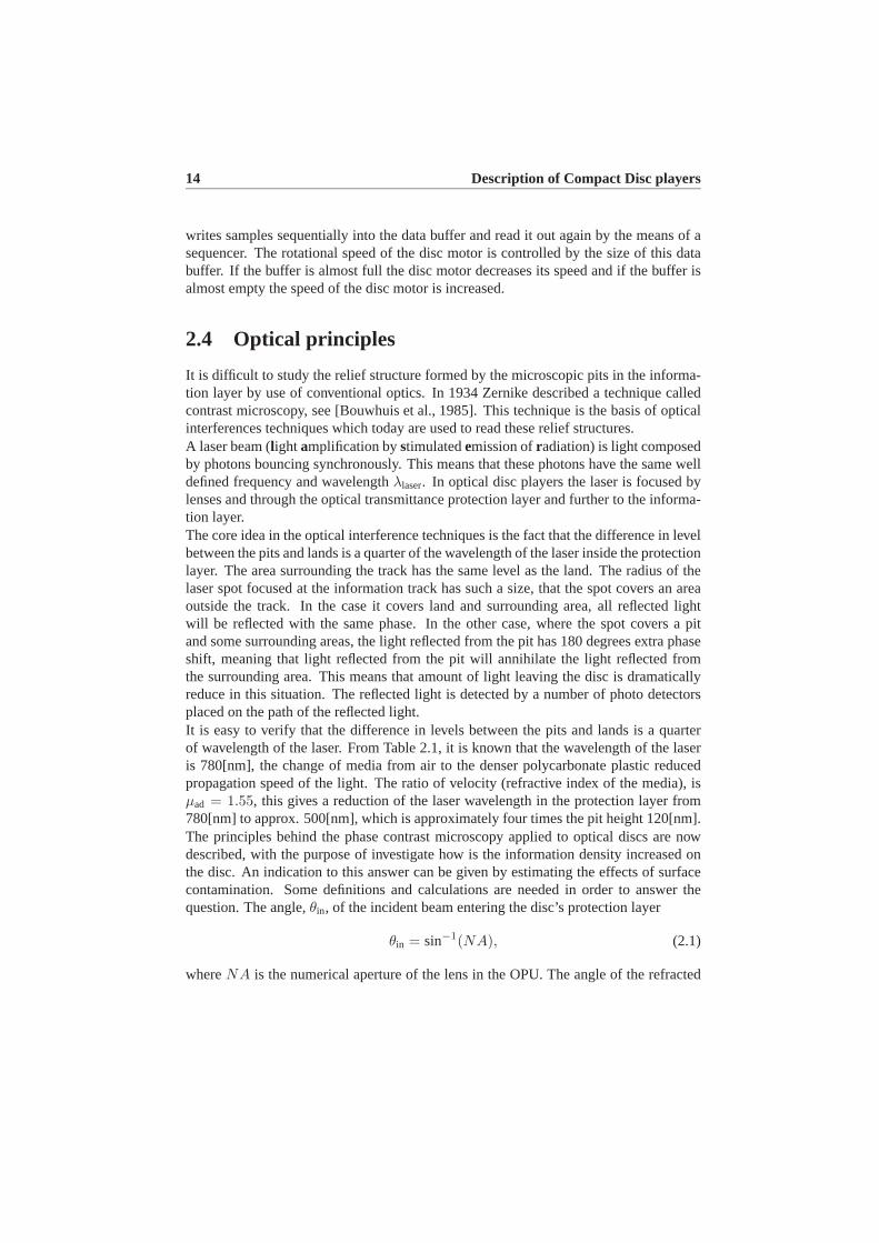
is too close, in middle the disc is in focus and at the bottom the disc is too far away. 182.7 Illustration of the Single Foucault focus detector principle. For simplicity this
illustration is based on point source laser, the principle in real world lasers is thesame. . . . . . . . . . . . . . . . . . . . . . . . . . . . . . . . . . . . . . . . 19
2.8 An illustration of some focus optical mappings.. . . . . . . . . . . . . . . . . 202.9 Illustration on how the three beams are positioned relative to each other on the
disc surface. . . . . . . . . . . . . . . . . . . . . . . . . . . . . . . . . . . . 212.10 Graphic representation of the maximum focus and radial deviations on CD. . . 242.11 Illustration of the main disturbances and defects affecting the focus and radial
loops. . . . . . . . . . . . . . . . . . . . . . . . . . . . . . . . . . . . . . . . 252.12 Illustration of the structure of the feature based control scheme, to handle surface
faults as faults.sm is vector of the measured detector signals,α is a vector of theresiduals,e is a vector of the static estimates of the distances,ff is a vector thefault features,e is a vector of the dynamical estimates of the distances,e is avector of the corrected distances,u is a vector of the control signals. . . . . . . 28
3.1 Overview of the experimental setup. . . . . . . . . . . . . . . . . . . . . . . . 333.2 Photo of the experimental test setup. . . . . . . . . . . . . . . . . . . . . . . . 343.3 Illustration of general model structure of the combined focus and radial model. . 363.4 Illustration of 2-axis device. . . . . . . . . . . . . . . . . . . . . . . . . . . . 363.5 Sketch of the driver part of the model.. . . . . . . . . . . . . . . . . . . . . . 37
xxi

xxii List of Figures
3.6 Free body diagram of the mass-spring-damper system.. . . . . . . . . . . . . 393.7 Illustration of the single Foucault focus detector principle. . . . . . . . . . . . 413.8 Illustration of the light intensity. . . . . . . . . . . . . . . . . . . . . . . . . . 423.9 Illustration on how the three beams are placed relative to each other.. . . . . . 433.10 The optical path with three lenses (f1, f2, f3) and a simplification. . . . . . . 453.11 Illustration on how the half disc is approximated.. . . . . . . . . . . . . . . . 463.12 Illustration on how much light emitted from the detector at heighthop is absorbed
by the knife. . . . . . . . . . . . . . . . . . . . . . . . . . . . . . . . . . . . 473.13 Illustration on how the reflected light covers the detector and area outside the
detector. . . . . . . . . . . . . . . . . . . . . . . . . . . . . . . . . . . . . . 483.14 Illustration of the laser spot placement over the track.. . . . . . . . . . . . . . 503.15 Illustration of the laser spot placement over the track.. . . . . . . . . . . . . . 513.16 Measurements off1(c · ef , 0) andf2(c · ef , 0). . . . . . . . . . . . . . . . . . 523.17 The focus detector as a function of the radial distance.. . . . . . . . . . . . . . 533.18 The radial detector as functions of the focus distance.. . . . . . . . . . . . . . 543.19 An illustration of the comparison of the measured and simulated radial detectors
dependence of the radial distances. . . . . . . . . . . . . . . . . . . . . . . . . 543.20 AD1 + D2 sequence of a scratchy disc, notice the spikes which are the scratches. 553.21 A 2-dimensional illustration of the disturbance set.. . . . . . . . . . . . . . . 563.22 A 2-dimensional illustration of an orthogonal fault model.. . . . . . . . . . . 563.23 A 2-dimensional illustration of a scaling fault model.. . . . . . . . . . . . . . 57
4.1 3-D plot ofβf in sequential fault encounters.. . . . . . . . . . . . . . . . . . . 614.2 The principles of the model of the CD-player.. . . . . . . . . . . . . . . . . . 614.3 The structure of the method described in this chapter. . . . . . . . . . . . . . . 624.4 Due to a fault the measured detector signal,sm, lies outside the output set of the
optical model. . . . . . . . . . . . . . . . . . . . . . . . . . . . . . . . . . . 624.5 Illustration of the principles of the scaling projection method.. . . . . . . . . . 644.6 Simulated optical detector signals without faults.. . . . . . . . . . . . . . . . 664.7 The focus and radial residualsαf andαr time series. . . . . . . . . . . . . . . . 674.8 Simulation of the four detector signals,D1[n], D2[n], S1[n] andS2[n], with
surface faults and measurement noises. . . . . . . . . . . . . . . . . . . . . . 684.9 Estimation of the four detector signals,D1, D2, S1 andS2 by the use of the
scaling projection method.. . . . . . . . . . . . . . . . . . . . . . . . . . . . 694.10 Bode plot of the Kalman estimator’s transfer function.. . . . . . . . . . . . . . 714.11 The statically and dynamically estimated focus distance signals.. . . . . . . . 714.12 The static and dynamic estimated radial distance signals.. . . . . . . . . . . . 724.13 Measured detector signalsD1[n], D2[n], S1[n] and S2[n] while passing the
scratch. . . . . . . . . . . . . . . . . . . . . . . . . . . . . . . . . . . . . . . 734.14 αf plotted together with detection signals. . . . . . . . . . . . . . . . . . . . . 744.15 αr plotted together with detection signals . . . . . . . . . . . . . . . . . . . . 74
5.1 The time-frequency plane of the Dirac basis in the discrete case.. . . . . . . . 785.2 The time-frequency plane of the Fourier basis in the discrete case.. . . . . . . 785.3 The time-frequency plane of the Short Time Fourier basis in the discrete case. . 805.4 The time-frequency plane of a Wavelet basis in the discrete case.. . . . . . . . 81
List of Figures xxiii
5.5 Principle time-frequency plane of an example of a Wavelet packet basis in thediscrete case. . . . . . . . . . . . . . . . . . . . . . . . . . . . . . . . . . . . 81
5.6 Illustration of the cascade filter implementation of the wavelet transform. . . . . 845.7 The mother wavelet and scaling function of the Daubechies 1-4, wavelets. . . . 855.8 Illustration of the cascade filter implementation of the wavelet packet transform. 865.9 Illustration of the possible basis of a wavelet packet tree of 3 levels. . . . . . . 875.10 An illustration of the best basis search.. . . . . . . . . . . . . . . . . . . . . . 895.11 Windowing functions. . . . . . . . . . . . . . . . . . . . . . . . . . . . . . . 915.12 The local cosine and the window function.. . . . . . . . . . . . . . . . . . . . 91
6.1 βf of a small scratch from a number of encounters of the same fault.. . . . . . 956.2 Illustration of the eye shaped scratch. . . . . . . . . . . . . . . . . . . . . . . 966.3 An example on Fang’s algorithm for segmentation of the time axis. . . . . . . . 976.4 An illustration of the first fault in the residual and theAFC(n) of the residual. . 986.5 An illustration of the second fault in the residual and theAFC(n) of the residual. 996.6 An illustration of the second fault in the residual and theAFC(n) of the residual. 996.7 The two residualsαf [n] andαr[n] computed for a disc with a scratch and a skew-
ness problem. . . . . . . . . . . . . . . . . . . . . . . . . . . . . . . . . . . . 1016.8 Illustration of the skewness of the disc. . . . . . . . . . . . . . . . . . . . . . 1026.9 The skewness component is removed from the two residuals.. . . . . . . . . . 1026.10 The two residuals computed of sampled signals with surface faults and eccen-
tricity problems. . . . . . . . . . . . . . . . . . . . . . . . . . . . . . . . . . 1046.11 The part of the tree of variance ofαf . . . . . . . . . . . . . . . . . . . . . . . 1076.12 The frequency amplitude plot of filter consisting of three times Haar low-pass
filtering followed by one time Haar high-pass filtering.. . . . . . . . . . . . . 1076.13 The part of the tree of variance ofαr. . . . . . . . . . . . . . . . . . . . . . . 1086.14 The frequency amplitude plot of a filter consisting of two times Haar low-pass
filtering followed by one time Haar high-pass filtering.. . . . . . . . . . . . . 1096.15 The output of using the joint best basis wavelet filters to locate the faults.. . . . 1096.16 A zoom on a scratch inef [n] filtered with three Haar low-pass filters followed by
one high-pass filter. . . . . . . . . . . . . . . . . . . . . . . . . . . . . . . . . 110
7.1 Illustration of the Karhunen-Loève approximation ofαf which contains a typicalscratch. . . . . . . . . . . . . . . . . . . . . . . . . . . . . . . . . . . . . . . 117
7.2 The 8 generalised Haar basis vectors.. . . . . . . . . . . . . . . . . . . . . . 1187.3 Illustration of the decision rule of the discriminator. . . . . . . . . . . . . . . . 1197.4 Illustration of the Karhunen-Loève approximation ofef + mn,f which contains a
typical scratch. . . . . . . . . . . . . . . . . . . . . . . . . . . . . . . . . . . 123
8.1 Illustration of the structure of the CD-player simulations model.. . . . . . . . 1278.2 Bode plot of the nominal focus controller.. . . . . . . . . . . . . . . . . . . . 1298.3 Bode plot of a focus controller with lower bandwidth. . . . . . . . . . . . . . . 1308.4 The upper plot is a zoom on a surface fault inef , for both controllers. . . . . . . 132
9.1 Illustration of the signals used the feature based control. . . . . . . . . . . . . . 1389.2 Illustration on the fault location and the interval in which the fault is located. . . 1409.3 Illustration of the feature based control scheme illustrated as a state machine. . . 140

xxiv List of Figures
9.4 Illustration of the closed loop with the feature based correctionP. . . . . . . . 1429.5 Closed loop of the feature based control system. . . . . . . . . . . . . . . . . . 1449.6 Simulations of the fault accommodation based onem − e handling a scratch. . . 1469.7 Simulations of the fault accommodation based onem handling the a scratch. . . 1469.8 A plot of the measured normalised focus difference, while the feature based cor-
rection algorithm is applied with the use of prediction of the fault location. . . . 1489.9 A plot of the measured normalised focus difference while the correction algo-
rithm is applied with the use of fault detection. . . . . . . . . . . . . . . . . . 1499.10 A zoom on the 1st and 5th encounter of the fault shown in Fig. 9.9.. . . . . . . 1509.11 A plot of the measured normalised radial difference while the fault correction
algorithm is applied with the use of thresholding in a predicted interval. . . . . 1509.12 A zoom on the 2nd and 4th encounter of the fault shown in Fig. 9.11.. . . . . . 151

List of Tables
2.1 The most interesting specifications in the CD, DVD and BRD standards. . . . . . 122.2 The calculated optical parameters for CD, DVD and BRD. . . . . . . . . . . . . 152.3 Standardised focus deviations from nominal position of the information layer. . . 232.4 Standardised radial deviations from nominal position of the information layer. . . 24
5.1 The number of possible bases in the wavelet packet tree for 1-8 levels.. . . . . . 87
6.1 The four examples of the time localisation based on the proposed methods. . . . 1056.2 The time localisation of the four scratch examples. . . . . . . . . . . . . . . . . 110
7.1 The results of the discriminator based on the 3 to 6 most discriminating Karhunen-Loève basis vectors are shown in this table. . . . . . . . . . . . . . . . . . . . . 120
7.2 The results of the discriminator based on 3 to 6 most discriminating Haar basisvectors are shown in this table. . . . . . . . . . . . . . . . . . . . . . . . . . . 121
7.3 The results of the discriminator based on the mean of class set of the order 3, thisset has only 3 vectors, shown in this table. . . . . . . . . . . . . . . . . . . . . 121
8.1 Table of the fault handling performanceDP and the nominal performanceNP. . 132
9.1 Table of the fault handling performanceDP, for both the feature based controlmethods.. . . . . . . . . . . . . . . . . . . . . . . . . . . . . . . . . . . . . . 147
B.1 Identified parameters inh1(·) andh2(·). . . . . . . . . . . . . . . . . . . . . . 168B.2 Identified parameters inh3(·) andh4(·). . . . . . . . . . . . . . . . . . . . . . 169B.3 Identified parameters ing1(·). . . . . . . . . . . . . . . . . . . . . . . . . . . . 169B.4 Identified parameters ing3(·) andg4(·). . . . . . . . . . . . . . . . . . . . . . . 170
xxv


Chapter 1
Introduction
Compact Disc (CD) players have been on the market since the beginning of the eighties,and now every home has at least one CD-player. The development of CD-players havebeen carried out through a number of different research areas. One of these areas iscontrol engineering. This research area together with signal processing is the main partof this thesis, and these areas are used to improve the CD-player’s aviability to play CDwith surface faults like scratches.
In Section 1.1 the problem of handling surface faults in CD-players are shortly describedand motivated. A overview of previous related work is given in Section 1.2. The problemdealt with in this project and how it is done is described in Section 1.3, the contributionsof this Ph.D project are presented in Section 1.4. An outline of this thesis is given inSection 1.5.
1.1 Motivation of the problem
The music is retrieved from the CD by the use of an Optical Pick-Up. This Optical Pick-Up has no physical contact with the data track on the CD. Therefore control is needed forthe Pick-Up to follow the track and to focus the laser beam at the track. By use of smartoptics the Pick-Up generates approximations of position errors of the Pick-Up relativeto the track. This sensor strategy is very usable in cases of healthy CDs, but if surfacefaults occur on the disc, these faults will influence the position sensor signals. In otherwords during surface faults it is not a good strategy to rely on the position sensors, orat least fully rely on them. This is in conflict with the specification of the controller forhandling disturbances like mechanical shocks etc, which the controller should suppressmeaning that a high bandwidth is needed. The idea of this Ph.D project is to solve thisnon-trivial problem of handling both surface faults and disturbances at the same time.
1
2 Introduction
1.2 Overview of previous and related work
CD-players have been on the market since 1982, where Philips and Sony launchedtheir first players. However the publication of research results on control of CD-players was delayed with a decade. From the beginning of the nineties research incontrol of CD-players has been intense, especially in the usage of adaptive and ro-bust controller. [Steinbuch et al., 1992] is the first example on aµ-controller to aCD-player based on DK-iterations. An example of an adaptive control design is[Draijer et al., 1992] where a self-tuning controller is suggested. In the followingyears a large number of different control strategies were applied to the CD-players.[Dötch et al., 1995] suggested an adaptive repetitive method, quantitative feedback the-ory is suggested in [Hearns and Grimble, 1999], rejection of non/repeatable distur-bances is suggested in [Li and Tsao, 1999], fuzzy control is used in [Yen et al., 1992],hybrid fuzzy control is used in [Yao et al., 2001], linear quadratic Gaussian con-trol is used in [Weerasooriya and Phan, 1995] and disturbance observer is used in[Fujiyama et al., 1998]. [Wook Heo and Chung, 2002] uses vibration absorber to dampthe mechanical disturbances.The development of DVD-players has implied some attention to this application. In[Zhou et al., 2002] sliding mode control is used to improve the performance against me-chanical disturbances if compared with a traditional PID controller. [Filardi et al., 2003]applied a robust control strategy to the DVD-player. [Zhu et al., 1997] uses iterativelearning control to perform the radial tracking in a DVD-player.The research is still focused on the CD-player application, this is illustrated in Ph.Ddissertations finished from the late nineties to now. [Dötsch, 1998] studied systemidentification for control design in CD-players, and in the same year [Lee, 1998] usedCD-players as a case study in his study of robust repetitive control. More recently,[Dettori, 2001] used LMI techniques to solve: multi-objective design and gain schedul-ing. [Vidal Sánchez, 2003] dealt with two problems, uncertainties of the CD-player bythe use ofµ-control and implementation of a controller tolerant towards surface faults.A clear majority of the research done in the area of optical drives is focused on min-imising the disturbances channel from mechanical disturbances/disc deviations to theposition error. Only [Vidal Sánchez, 2003] addresses the problem of handling surfacefaults such as scratches, fingerprints etc. The surface faults impose an upper limit onthe controller bandwidth, which is in conflict with the minimisation of the disturbanceschannels, since minimisation of the disturbances require high controller bandwidths.[Heertjes and Sperling, 2003] and [Heertjes and Steinbuch, 2004] indirectly handle thesurface faults by the use of non-linear filters to improve controller sensibility withoutmaking the controllers more sensitive towards the surface faults.
1.2.1 Background at Aalborg University
In 1997 Department of Control Engineering at Aalborg University and Bang & Olufsenstarted a co-operation in advanced control of CD-players. The start was a master stu-

1.3 Basic idea of the Ph.D project 3
dent project, see [Vidal et al., 1998]. This student project showed the need for a largerresearch project (OPTOCTRL). OPTOCTRL dealt with the use of advanced controltechniques for improving the reproduction of sound in CD-players. This was the subjectof Enrique Vidal Sánchez’s Ph.D thesis [Vidal Sánchez, 2003], and in a number of stu-dent projects. OPTOCTRL did also host a project of low cost optical active sensors, see[la Cour-Harbo, 2002]. In this work joint time and frequency based methods were usedto improve optical detectors. In [Vidal Sánchez, 2003] it was concluded that the use ofadvanced control techniques can improve quality of reproduced sound in case of faultson the CD surface.In 2001 another research project was founded partly based on OPTOCTRL. This projectcalled Wavelets in Audio/Visual Electronics Systems (WAVES), contains a work pack-age handling surface faults on CDs with the use of joint time/frequency based featureextraction to improve the advanced controllers. This Ph.D project that makes the basisof this thesis is the work packages (Feature based control of Optical Disc players).
1.3 Basic idea of the Ph.D project
The idea is to handle the surface faults such as scratches and fingerprints without de-creasing the suppression of disturbances. This can be achieved by viewing this controlproblem of handling surface faults in CD-players as a fault tolerant control problem,where the surface faults are viewed as fault which can be handled by the use of an ac-tive fault tolerant controller, where the surface defects components are removed fromthe measurement signals. This adaption are done by the use of feature extraction ofthe defect, where time-frequency analysis method are used to extract these features, see[Mallat, 1999].
1.4 Contributions
In the following list the main contributions of the author are summarised, most of thesecontributions have been or are going to be published in international conference pro-ceedings and international journals.
• A model of the optical detector system, including cross-couplings between focusand radial detectors see [Odgaard et al., 2003c]. This model is non-linear andshows a clear coupling between focus and radial detectors.
• A method for computing the locally defined inverse map of the optical model ispresented in [Odgaard et al., 2004a]. This computes a static estimates of focusand radial positions and decoupled residuals for detection of surface faults.
• A Kalman estimator is used to compute dynamical estimates of focus and ra-dial positions based on the static estimates, see [Odgaard et al., 2003b] and[Odgaard et al., 2003a].

4 Introduction
• An advanced version of the threshold method is developed in order to improvethe time localisation of the surface faults, [Odgaard and Wickerhauser, 2004],based on the decoupled residuals. In addition two time-frequency based meth-ods are designed based on Fang’s algorithm, [Odgaard and Wickerhauser, 2004],and wavelet packet filters, [Odgaard et al., 2004e].
• A local discriminating basis is found, the most discriminating basis vec-tors of this basis are used to discriminate among different classes of faults,[Odgaard and Wickerhauser, 2003]. The members of these defect classes can beapproximated by use of a few most approximating Karhunen-Loève basis vectors[Odgaard and Wickerhauser, 2003]. The coefficients as well of these basis vectorsare the extracted features.
• A model of surface faults is formed see [Odgaard et al., 2003a] and[Odgaard et al., 2004d]. This model can be used to design Fault Toler-ant Controllers, and to simulate CD-player playing a disc with surfacefaults [Odgaard et al., 2004d]. This model is implemented in MATLAB ,[Odgaard et al., 2003d].
• A Fault Tolerant Control scheme is developed. This scheme handles sur-face faults by the use of the extracted features [Odgaard et al., 2004c] and[Odgaard et al., 2004b].
1.5 Outline
The remaining parts of the thesis are organised as follow:
Description of Compact Disc players introduces the Compact Disc technologyfor the reader. Other optical disc formats are also introduced to give an idea ofwhy the result achieved at the CD-players can be generalised to other disc formats.The Optical Pick-Up and positioning servos are described and explained. Finallythe interesting control problems in the CD-player are discussed and explained.This leads to a proposed structure of the feature based controller scheme.
Model of Compact Disc players introduces and describes the Test Setup usedin this work. This is followed by a description of the overall model structure andmodel of CD-player containing the dynamical model of the electro-magnetic part,the non-linear static model of the optical part and a model of surface faults.

1.5 Outline 5
Fault Residuals based on Estimations of the Optical model derives a local so-lution to inverse map of the combined optical model of the CD-player and modelof the surface faults. The solution gives estimates of the fault parameters (residu-als) and the actual position of the optical pick-up.
Time-Frequency analysis introduces some relevant time-frequency theoriesand bases, these theories and bases are of large importance in the remainder ofthis thesis.
Time localisation of surface faults describes three developed methods for lo-cating and detecting the surface faults. These methods uses the new derived faultresiduals as the basis of the localisation and detection of the surface faults. Thethree methods are based: on Fang’s algorithm for segmentation of the time axis,joint best basis wavelet packet filters and en extended version of the normally usedthresholding method. These methods are all validated by the use of experimentaldata.
Time-frequency based feature extraction of Surface Faults describes thegeneral idea of extracting features, especially is given an explanation of whichfeatures are interesting for the control of the CD-player. Two different kinds offeatures are extracted: class of fault, and approximating coefficients.
A Simulation model develops a simulation model of CD-players playing discswith defective surfaces. This simulation model is based on a model of a CD-player, the model of surface faults, and time-frequency based features extracted inthe previous chapter.
Feature based control of Compact Disc players describes the basic idea of thisfeature based control scheme. The scheme is related to the general fault tolerantcontrol scheme. Moreover this control scheme is derived based on the extractedfeatures of surface fault. These features are used in order to remove the faultsinfluence on the positioning servos. Stability issues of the scheme is discussedand the scheme is proven to be stable. Finally the scheme is validated throughsimulations and experimental tests.
Conclusion gives concluding remarks on this thesis and some suggestions forfuture work in this field.


Chapter 2
Description of Compact Discplayers
In this chapter the optical disc player in general and the CD-player in particular aredescribed. This description makes it possible to identify the challenging control prob-lems in the optical disc players. This leads to a description of the main topic in thisPh.D project: handling of surface defects based on a feature based fault tolerant controlscheme. In Section 2.1 the different optical disc formats are described, this leads to adescription of the optical discs, see Section 2.2. In Section 2.3 the optical disc playeris described. Some basic optical principles are the topics in Section 2.4. These princi-ples are used to compare the different kinds of optical disc formats, which are followedby the basics in the optical pick-up, see Section 2.5. In Section 2.6 some of the mostused optical measurement principles are described. The servo loops are described inSection 2.7. In Section 2.8 the performance requirements, disturbances and defects arediscussed. Finally, in Section 2.9 the specific fault tolerant control scheme used in thiswork is described.
2.1 Optical disc formats
Even though this thesis is focused on the Compact Disc (CD), the most well knownoptical disc formats will shortly be described and compared to the CD. The first opticaldata storage technique was announced by Philips in 1972. The first optical discs wereanalog optical discs see [Bouwhuis et al., 1985]. Almost a decade later in 1981 Philipsand Sony proposed a digital standard, the Compact Disc Digital Audio standard (CD-DA), which was coded in the so-called red book [Philips and Sony Corporation, 1991].The year after in 1982 Philips and Sony launched their first CD-players on the market.Almost 10 years later in 1991 the sale of CDs exceeded the sale of audio-cassettes, and
7

8 Description of Compact Disc players
the long play records, its predecessor as the high quality music storage media.In addition to audio application of CDs, the CDs have also been developed in otherversions for other applications. The most well known other application is for binarydata storage on computers, CD-ROM. Another application is CD-video where the CDmedia is used to storage videos, movies etc. The CD-videos have never conquered alarge part of the video market, since one disc with the in the standard used compressioncannot contain an entire movie. To day with the use of standard computers and newcompression algorithms it is possible to store an entire movie on a CD-ROM. Todaysfast computers can decompress and play the stored movie in real-time.The next generation of optical disc players, the Digital Video/Versatile Disc (DVD) hasthe capacity to store an entire movie in a good quality on one disc. A CD has the storagecapacity of 650/700 MB and the DVD upto 25 times as much. The DVD can be used forthe three applications audio, video and ROM as well as the CD.The generation of optical discs which are the successors of the DVD is now in the phaseof development, this type of optical discs are typically called High Density OpticalDiscs. For the time being four different standards have been proposed, with a typi-cally storage capacity from 20 GB to 50 GB. (Approximately 30 to 75 times the CDcapacity). These four standards are: the Blu-ray disc (BRD)[Hitachi, Ltd. et al., 2002],the advanced optical disc [Toshiba Corporation and NEC Corporation, 2002], the Blue-HD (High Density) disc [AOSRA, 2003] and the HD-DVD-9 disc [Warner Bros, 2002].They are all re-writable discs.In addition to the large variety of disc types, the CD and DVD are available in a massreplicated moulded disc, Write Once Readable Memory (WORM), and re-writable discs.These different types of discs are shortly described below.
Mass replication moulded discs These discs are prerecorded CDs or DVDs contain-ing audio, video or data. The information is stored on these discs in a mass duplicationprocess by the use of stamping. This stamped surface is following coated with an ultrathin layer of reflective material such as copper, aluminium, gold or silver. The produc-tion of the disc is finalised with a layer of transparent protection material. It is clear fromthe description that this disc cannot be re-recorded.
WORM discs These Write Once Read Many times discs are a group of discs con-taining a recordable CD (CD-R) and a recordable DVD (DVD-R). These discs are inmany ways much alike the first group of discs, but deviate in one important way. Theyhave a layer of photosensitive dye covered by a reflective metallic layer. The discs arerecorded by burning the photosensitive material in the dye by a laser. This process is notreversible and only durable once, meaning this burning is permanent.
Re-writable discs In these discs the WORM discs’ photosensitive dye layer is re-placed with a special phase-change compound. The phase of this compound can be

2.2 The optical disc 9
changed due to the amount of energy applied by the laser. This means that it is possi-ble to erase and rewrite the disc. These discs lifetime measured in numbers of rewrit-ings varies from a 1000 times (CD-RW, DVD-RW, DVD+RW) to 100,000 times (DVD-RAM). All the proposed High Density discs are in principle re-writable. However, ROMversions of the High Density discs are being discussed.
These descriptions give a brief overview of the wide variety of optical discs on themarket, this overview is illustrated in Fig. 2.1. The competition of the leading positionon the re-writable DVD market has not declared a winner yet. One could say that thecompetition on the High Density disc marked has not really started, since the competingstandards have not been completely established. The optical principles behind all thesediscs are similar. In the following sections these principles are described by focusing onCDs. During this description some of the important differences between the differentkinds of discs are mentioned.
Mass replication
optical discsRe−writable
WORM discs
moulded discs
High Density Optical Discs
DVD−RW
DVD+RW
DVD−RAM
DVD−R
DVD−ROM
DVD−VIDEO
DVD−AUDIO
CD−RW
CD−R
CD−AUDIO
CD−VIDEOCD−ROM
Figure 2.1: The most common types of optical discs. CDs, DVDs and HDs grouped intodisc production types.
2.2 The optical disc
The diameters of the CD and the DVD are for both 120 mm, some of the HD discs aresmaller, and some of them do have a diameter on 120 mm. The data is on all discsstored in a clockwise spiral track starting from the centre of the disc. The spiral consistsof microscopic pits. The length of the pits and the area between them form the recorded
10 Description of Compact Disc players
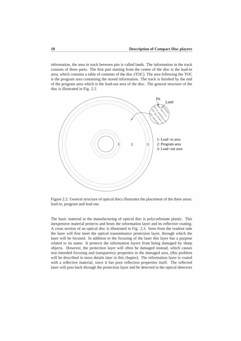
information, the area in track between pits is called lands. The information in the trackconsists of three parts. The first part starting from the centre of the disc is the lead-inarea, which contains a table of contents of the disc (TOC). The area following the TOCis the program area containing the stored information. The track is finished by the endof the program area which is the lead-out area of the disc. The general structure of thedisc is illustrated in Fig. 2.2.
1 2 3
LandPit
1: Lead−in area2: Program area3: Lead−out area
Figure 2.2: General structure of optical discs illustrates the placement of the three areas:lead-in, program and lead out.
The basic material in the manufacturing of optical disc is polycarbonate plastic. Thisinexpensive material protects and hosts the information layer and its reflective coating.A cross section of an optical disc is illustrated in Fig. 2.3. Seen from the readout sidethe laser will first meet the optical transmittance protection layer, through which thelaser will be focused. In addition to the focusing of the laser this layer has a purposerelated to its name: It protects the information layers from being damaged by sharpobjects. However, the protection layer will often be damaged instead, which causesnon intended focusing and transparency properties in the damaged area, (this problemwill be described in more details later in this chapter). The information layer is coatedwith a reflective material, since it has poor reflection properties itself. The reflectedlaser will pass back through the protection layer and be detected in the optical detectors

2.3 The optical disc player 11
Reflective coat
Readout side
Information layer
layerprotectiontransmittanceOptical
Figure 2.3: Cross section of the disc. This disc has only one information layer as CDs,even though some other optical discs have several information layers.
(optical sensors). In dual layer DVDs the upper information layer is covered with a semi-reflective material, through which it is possible to focus the laser. In addition the upperlayer has a lower density compared to a conventional layer such as the lower layer. Byusing this lower density the Signal Noise Ratio (SNR) can be kept low. The side oppositethe readout side is normally called the label side where a label can be printed on the disc.But in case of a double sided discs this label has to be transparent for the laser beam.Some interesting key specifications of the different generations of optical discs arecompared in Table 2.1, based on [Philips and Sony Corporation, 1991], [ECMA, 2001],[Hitachi, Ltd. et al., 2002]. As a representative of the group of High Density opticaldiscs the Blu-Ray Disc (BRD) is chosen. Other standards in this group may have otherspecifications. All the HD discs standards except HD-DVD-9, increase the informationdensity by the use of blue lasers. The HD-DVD-9 increases the density by use of a moreefficient data coding algorithm.
2.3 The optical disc player
A block diagram of the optical disc player is shown in Fig. 2.4. This block diagramillustrates the most important parts of an optical disc player. The OPU is the OpticalPick-up Unit which emits and focus the laser at the disc surface, it also detects the laserbeam reflected back from the information layer in its photo detectors. The remaining sy-stem can naturally be divided into three subsystems: the data path, control/servo systemand the logic block. The logic block serves the role as being interface between the userand the servo part and performs the required logic in order to keep the correct sequencesof operation. The purposes of the two other subsystems can shortly be described. The

12 Description of Compact Disc players
CD DVD BRD
Disc Diameter [mm] 120 120 120Disc thickness [mm] 1.2 1.2 1.2Tracking pitch [µm] 1.6 0.74 0.32Optical transmittance 1.17 0.6 0.1protection layer [mm]Laser wavelength [nm] 780 (infrared) 650 (red) 405 (blue-violet)Numerical aperature (NA) 0.45 0.6 0.85Air/disc refractive index (µad) 1.55 1.55 1.55Data layers 1 1 or 2 1 or 2Readout sides 1 1 or 2 1 or 2Data capacity [GBytes] 0.65 or 0.7 4.7-17.0 23.3-50
Table 2.1: The most interesting specifications in the CD, DVD and BRD standards.The BRD has been chosen as an example of the High Density Disc standards, as thespecifications are available at this time.
control/servo system has to positing the OPU such that it can generate some signals de-pending on the information stored in the information layer. The job of the data path is toconvert these retrieved signals into the data stored in the information layer. The sledgeservo moves the OPU for coarse radial adjustments and focus and radial servos are usedfor fine positing of the OPU. The disc motor has the important function to spin the discaround at the adequate speed.
The OPU generates the self-clocking waveform data from the disc. This signal is re-ferred to as High Frequency (HF) signal. This signal can be coded in different waysdepending on the type of disc. In CDs the Eight-to-Fourteen Modulation (EFM) chan-nel code is used for coding the data. 8 bit data are represented on the disc by 14 channelbits plus 3 additional bits. The length of the pits and lands is in the interval from 3 chan-nel bits to 11 channels bits, see [Stan, 1998]. The DVDs use an advanced version of theEFM coding called EFM+, where the 8 data bits are represented by 17 channel bits onthe disc. The Data Separator separates the HF signal into: subcode bytes, data samples,clock signal. The subcode is a kind of a time stamp on each data sample, which is usedby the logic unit to locate the required data samples in the correct order. The PLL lockis used to decode the EFM signal, for more information see [Stan, 1998].
The separated data samples are fed to the Error Corrector, in which the redundant dataare used to check and eventually correct erroneous data. The error correcting methodin CDs is Cross Interleaved Reed-Solomon code (CIRC). This error correction methodis based on the work by Reed and Solomon, see [Reed and Solomon, 1960]. Its maxi-mum correction length is 4000 bits which are approximately 2.5[mm] track. The Reed-Solomon (RS) product code, a variant of the CIRC, is used for error correction in DVDs,is capable of handling errors relating to approximately 6[mm] track. The deinterleaver

2.3 The optical disc player 13
Disc
motorDisc
SledgeOPU
unit Interface
and deinterleave
Data buffer
(variable bit rate)
DataVideoAudio
PLL Lock
SubcodeUser
Error correction
Logic
separatorData
movementsSledge
adjustRadial
Focus adjust
motor
Radialservo servo
Discservo
SledgeFocusservo
Figure 2.4: A block diagram of general structure of the optical disc player. The broadarrows illustrate the data path, and the narrow arrows handling and control. The dashedarrows are logical signals which handles special operations, such as start-up, track jumpetc. The OPU is the Optical Pick-up Unit which is used to emit and detect the laserbeam.
14 Description of Compact Disc players
writes samples sequentially into the data buffer and read it out again by the means of asequencer. The rotational speed of the disc motor is controlled by the size of this databuffer. If the buffer is almost full the disc motor decreases its speed and if the buffer isalmost empty the speed of the disc motor is increased.
2.4 Optical principles
It is difficult to study the relief structure formed by the microscopic pits in the informa-tion layer by use of conventional optics. In 1934 Zernike described a technique calledcontrast microscopy, see [Bouwhuis et al., 1985]. This technique is the basis of opticalinterferences techniques which today are used to read these relief structures.A laser beam (light amplification bystimulatedemission ofradiation) is light composedby photons bouncing synchronously. This means that these photons have the same welldefined frequency and wavelengthλlaser. In optical disc players the laser is focused bylenses and through the optical transmittance protection layer and further to the informa-tion layer.The core idea in the optical interference techniques is the fact that the difference in levelbetween the pits and lands is a quarter of the wavelength of the laser inside the protectionlayer. The area surrounding the track has the same level as the land. The radius of thelaser spot focused at the information track has such a size, that the spot covers an areaoutside the track. In the case it covers land and surrounding area, all reflected lightwill be reflected with the same phase. In the other case, where the spot covers a pitand some surrounding areas, the light reflected from the pit has 180 degrees extra phaseshift, meaning that light reflected from the pit will annihilate the light reflected fromthe surrounding area. This means that amount of light leaving the disc is dramaticallyreduce in this situation. The reflected light is detected by a number of photo detectorsplaced on the path of the reflected light.It is easy to verify that the difference in levels between the pits and lands is a quarterof wavelength of the laser. From Table 2.1, it is known that the wavelength of the laseris 780[nm], the change of media from air to the denser polycarbonate plastic reducedpropagation speed of the light. The ratio of velocity (refractive index of the media), isµad = 1.55, this gives a reduction of the laser wavelength in the protection layer from780[nm] to approx. 500[nm], which is approximately four times the pit height 120[nm].The principles behind the phase contrast microscopy applied to optical discs are nowdescribed, with the purpose of investigate how is the information density increased onthe disc. An indication to this answer can be given by estimating the effects of surfacecontamination. Some definitions and calculations are needed in order to answer thequestion. The angle,θin, of the incident beam entering the disc’s protection layer
θin = sin−1(NA), (2.1)
whereNA is the numerical aperture of the lens in the OPU. The angle of the refracted

2.4 Optical principles 15
CD DVD BRDIncident angleθin [◦] 27 37 58Refracted angleθout [◦] 17 23 33Readout beam sizeDbeam[mm] 0.72 0.51 0.13Focused beam size at information layerdtrack [µm] 0.87 0.54 0.24
Table 2.2: The calculated optical parameters for CD, DVD and BRD.
beam can be computed by
θout = sin−1
(sin(θin)
µad
), (2.2)
whereµad is the refraction index which can be seen in Table 2.1. [Bouwhuis et al., 1985]gives the diameter of the focused laser spot at the information track,dtrack,
dtrack =λlaser
2 · NA. (2.3)
After computing the spot diameter at the information track it is possible by the use ofgeometric computations to compute the diameter of the readout beam,Dbeam, at the discsurface. It is given by the following equation
Dbeam=2 · Tl
tan(90◦ − θout)+ dtrack [m], (2.4)
whereTl is the thickness of the protection layer, and is given in Table 2.1.The density of information on an optical disc can be approximated, see[Bouwhuis et al., 1985] by
density=(
NA
λlaser
)2
, (2.5)
(2.5) indicates two possibilities to increase the information density on the optical disc,either by increasing theNA and/or decreasing the wavelength of the laser beam. In-creasing theNA and/or decreasingλlaser results in a decreased focused spot size. Theseoptical changes also introduce a side effect of an increased optical aberration (distor-tion), which is compensated by reducing in thickness of the optical transmittance pro-tection layer. One consequence of the reduction of thickness of the optical transmittanceprotection layer, is clear. The maximum depth of a scratch in the disc surface withoutdamaging the information layer is decreased as the thickness of the optical transmittanceprotection layer decreases, since the laser spot size at the disc surface also decreases sur-face defects would appear larger as well. To study this phenomenon more detailed thefigures of the above principle calculations are performed for: CD, DVD and BRD, asrepresentative of the high density optical disc, see Table 2.2.

16 Description of Compact Disc players
Examples on some surface defects as dust particles and a human hair on the disc surfaceare by rule of thumb considered to be of the respective sizes: 40[µm] and 75[µm]. Bycomparing these sizes withDbeam of the different medias in Table 2.2 it is seen that ahair or a dust particle are not an obstacle in the readout on a CD, due to the high ratiobetweenDbeamand the size of the defect. This ratio decreases from CDs to DVDs wherethese kind of defects tend to be an obstacle in the readout process, and for the BRDthese defects are almost as large as the laser beam itself, and are thereby even a largerobstacle.
2.5 The optical pick-up
The standards of optical disc players do not describe much concerning the optical pick-up, they only give a set of requirements to the wave length of the laser beam and thenumerical apperature of the lens. These few requirements to the optical pick-up give alarge degree of freedom for the designers of the optical pick-up; as a consequence thegeneral principles will be described, and are illustrated in Fig. 2.5.The laser beam is emitted by the laser diode. The light beam will following meet anobjective lens before it meets a polarising prism with a defined transmittion plane. Thelight is following phase shifted with a phase of 90◦ in the Quarter-wave plane. The laserbeam is focus at the information layer by the use of the 2-axis moving objective lens;the light beam reflected back from the informations layer also passes through this lens.The quarter-wave plane again phase shifts the reflected light with 90◦. The light beamis following reflected in the polarising prism towards the photo diodes (photo detectors).An objective lens is used to focus the light beam at the photo diodes. An alternativeimplementation is to implement all the optical elements, except the 2-axis moving lens,laser and photo detectors in a hologram. In addition the laser and the photo detectors canbe placed in the same housing as the hologram, this implementation is often used sinceit is more environmentally and mechanically stable. The optical pick-up is in addition toreadout of data also used to measure the focus and radial distances. The implementationof these indirect measurements variates from players and design; some of the most usedprinciples are described in the next section. In the following the Optical Pick-up Unit,will be denoted as OPU.
2.6 Optical measurements
As a consequence of the lack of physical contact between the OPU and the optical discsurface, it is needed to measure the position of the OPU relative to the informationtrack in two directions: in the focus direction and in the radial direction. There is alarge variety in the methods and principles used for measuring these distances. In thefollowing some of the most used ones are shortly described, starting with the focusdistance measurements.

2.6 Optical measurements 17
����
����
��������
Disc
2−axis
lensmoving
Quarterwave plate
Polarisingprism
Lens
Laserdiode
PhotoDetectors
Hologram
��
�� ��
�� ��
��
Figure 2.5: The general principle of the optical pick-up.
2.6.1 Focus distance measurements
The four most used focus distance measurements are shortly described, starting withthe astigmatic principle, followed by single Foucault, double Foucault and spot-sizedetections. The general principles behind all these methods are to place some kind ofasymmetry in the path of light reflected from the disc.
Astigmatic principle The astigmatic principle is illustrated in Fig. 2.6. A cylindricallens is placed in front of the photo detectors. This lens has two focus points, one infront of the photo detectors and one behind them. The image of the laser beam on thephoto detectors will be an ellipse whose aspect ratio changes as a function of the focusdistances. In the cases of the focus distance being equal to zero, the image will becircular, since the cylindric lens is designed in such a way that zero focus distance is inbetween of the two foci of the cylindric lens. The focus distance is measured by dividingthe photo detectors into four quadrants. When these are connected as shown in Fig. 2.6the focus distance is computed. The data readout is the sum of the high frequency signal

18 Description of Compact Disc players
from all these four photo detectors. The mapping from the focus distance to astigmaticmeasurement of the focus distances is shown in Fig. 2.8 where it is compared with theSingle Foucault mapping.
+−
v>0
+−
+−
Disc in focusv=0
Disc too far
Disc too close
v<0
Figure 2.6: Illustration of the astigmatic principles. In the top an illustration where thedisc is too close, in middle the disc is in focus and at the bottom the disc is too far away.
Single Foucault principle The Single Foucault principle is also called the knife-edgemethod since a knife edge introduces the asymmetry in the light path. The light beamwill be detected by two photo detectors. The knife edge is placed in a position that givesboth photo detectors the same level of light energy in the case of zero focus distance, asillustrated in Fig. 2.7. In the cases where the light beams is out of focus, the knife edgewill change the ratio of detected light at the photo detectors, which is illustrated in Fig.2.8. The absorption of light increases as the numerical focus distance increases.Based on the description it is clear that the placement of the knife edge is highly impor-tant. Just a small misplacement can result in large measurement errors. This problem isoften solved by implementing the knife edge in a hologram together with the lenses.The mappings of the Single Foucault principle and the astigmatic principle are shownin Fig. 2.8. In principle these curves are different as in Fig. 2.8, see [Stan, 1998] and
2.6 Optical measurements 19
"In focus"
"Too far"
"Too close"
D1−D2=0
D1−D2<0
D1−D2>0
D2
D1
D2
D1
D1
D2
Figure 2.7: Illustration of the Single Foucault focus detector principle. For simplicitythis illustration is based on point source laser, the principle in real world lasers is thesame.
[Vidal Sánchez, 2003]. These assume, however, the Single Foucault photo detectors tobe of infinite size. This is of course not the case in real applications. The designers willoften choose to minimise these detectors. As the focus distance increases, the size ofthe laser spot both on the disc surface and photo detectors increases too. A consequenceof this is that the amount of energy detected decreases dramatically towards zero, see[Odgaard et al., 2003c] and Section 3.4.
Double Foucault principle In this principle the knife edge is replaced with a prism.The prism is used to split the light beam along the optical axis. Two pairs of photodetectors are used to obtain the distance error signal based on the split laser beam. TheDouble Foucault principle is rarely used, it is replaced by its counterpart the SingleFoucault principle, [Stan, 1998].
Spot-size detection principle This method also uses a prism and two split detectors,and is still used in some CD-ROM drives, [Stan, 1998]. This principle measures thechange in spot size since the spot size depends linearly on the focus distance.
2.6.2 Radial distance measurements
The radial distance can be measured in a number of ways. In the following some of themost commonly used ones are shortly presented.

20 Description of Compact Disc players
�����������������������
�����������������������
(2)
(1)
focus distance [m]de
tect
or d
iffe
renc
e [V
]
Figure 2.8: An illustration of the theoretical Single Foucault (1) and practically SingleFoucault and Astigmatic, (2), optical mappings.ef is the focus distance,u is the photodetector difference. Notice that these two method generates in theory different opticalmappings, the practically Single Foucault mappings is alike the Astigmatic mapping.
Three beams principle In addition to the main beam used for data readout and focusdistance measurements two additional laser beams are used. This method is also calledtwin-spot radial detection. The two additional laser beams are derived from the mainlaser beam by a grating structure, the side spots are placed aside the main beam, withan offsetak, as illustrated in Fig. 2.9. If a spot is fixed over the track, the received highfrequently photo detector signal will have an amplitude depending on the pits and landsin the track. However, a low frequently signal will be of constant value for a constantradial distance, since the sensor signals are low-passed filtered the pits and lands are notof any interest in this process of computing the radial distance. These can be removedfrom the photo detector signals by low-pass filtering these detector signals. When low-pass filtered, the radial error can be approximated by the difference between the two sidephoto detectors as illustrated in Fig. 2.9.
Track Wobble principle The idea behind this principle is to feed a sinusoidal signalto the radial servo, causing a radial oscillation of the radial distance of a few decades ofnanometers. This modulates the envelope of the readout signal. This modulation can beused to obtain the radial distance.
Push-pull principle The push-pull principle uses a diffraction pattern to analyse thereflected beam. In the case the OPU is out of radial tracking, (the radial distance differentfrom zero), one of the photo detectors will see larger pit/land modulation than the other.

2.7 Optical disc servos 21
Side spot
Side spot
Main spot
Track
S1
S2
er
er + ak
dtrack
Figure 2.9: Illustration on how the three beams are positioned relative to each other onthe disc surface.S1 andS2 are the two side detectors,dtrack is the track width,er is theradial distance, andak is the offset of the side detectors.
Differential time detection principle The three beams principle is often used in CD-players, where the two other principles mentioned above are also used. However, theyall have some severe disadvantages which disqualify them for use in DVD and HDdrives. Instead another method is preferred called Differential Time Detection (DTD),or a variant called Differential Phase Detection (DPD). The idea is to detect the time orphase change of the high-frequency signals as a function of the radial distance of thescanning spot. These time or phase changes arise in a four quadrant photo detector. Byprocessing the four signals detected in the four photo detectors the radial distance canbe obtained, for more details on DPD/DTD see [Braat et al., 2002]. In practise the DTDis used, since the measuring of the differential phase change is more complicated.
2.7 Optical disc servos
Servo loops are in the optical disc players used to control three states: focus and ra-dial distances and either the linear or angular speed of the OPU relative to the track.There is a number of different actuator configurations for the adjustment of focus andradial distances, see [Stan, 1998] and [Bouwhuis et al., 1985]. In the following only theconfiguration from the used CD-player is described. One servo is used to adjust focusdistance. This servo is called the focus servo. Two servos are used to handle the radialcorrections. The radial servo is used to do the fine adjustments of the radial distance andthe larger adjustments are handled by the sledge servo. Finally one servo controls thedisc speed.

22 Description of Compact Disc players
Focus servo A linear electro-magnetic actuator performs the corrections in the focusdistances, by positioning the moving lens in the focus direction. The control signalto the focus actuator is computed based on the focus distance measurement. Due tothe non-linearity of the focus measurement, it is of high importance to keep the focusdistance close to zero and at least in the linear area of the focus measurement mapping;for more details on the performance requirements see Section 2.8.1. The disturbanceswhich move OPU out of focus have many different natures, see Section 2.8.2. It isvery important to strongly suppress the disturbances, due to the small dimensions of thetrack, lands and pits. If the disturbance is not suppressed, the OPU will get out of focusand it is not possible to retrieve any information from the disc before the OPU has beenfocused again.
Radial servo The fine adjustments of the radial distances are performed in the sameway as the focus adjustments, except that the radial linear electro-magnetic actuatormoves the moving lens in the radial direction instead. The working range of the radialactuator is only a few hundred tracks, meaning that another servo is needed for the largercorrections in the radial directions, this servo is called the sledge servo, and will be de-scribed in the next paragraph. The focus and radial servos are designed to be decoupled,since the linear magnetic actuators are placed orthogonal to each other, however in prac-tise cross-couplings can occur, see [Dettori, 2001] and [Yeh and Pan, 2000]. For singlespeed optical disc drives such as the CD-Audio, these cross-couplings can be neglected.
Sledge servo The sledge servo performs the larger radial corrections by moving theOPU in the radial direction, as illustrated in Fig. 2.4. The OPU is mounted on this sledgewhich is driven by motorised gears enabling the movements of the OPU in the entireprogram area of the optical disc. Ideally the sledge servo performed slow continuousadjustments while the radial servo handles the high frequent adjustments, meaning thatthe sledge servo do not introduce perturbations on the radial position, or in other wordsdo disturb the radial servo. Unfortunately, this is not the case in practise, since where is aclear self-pollution in the radial servo originating from the sledge servo. Variations andimperfections in the sledge actuators can cause severe disturbances in the radial servo. Insome cases of severe disturbances these can result in a loss of track situation. The hierar-chy of the radial and sledge servos is often such that the sledge servo react on the radialcontrol signal if it is too large. [Aangenent, 2002] and [Dzanovic and Lauritsen, 2003]did some dedicated work on the cross-coupling between the radial and sledge servos.
Disc servo The data in optical discs are recorded using a constant channel clock. Asa consequence the disc servo should control the readout speed of the disc to be a Con-stant Linear Velocity (CLV) of 1.3 [m/s]). This results in a feeding of data to the dataseparator with a constant throughput at 150[Kb/s], also called 1xspeed. With CLV rota-tion frequency decreases from the lead in area to the lead out area (9[Hz]-3[Hz]). Therotation speed is in practise controlled by the use of fullness of a data buffer, which is
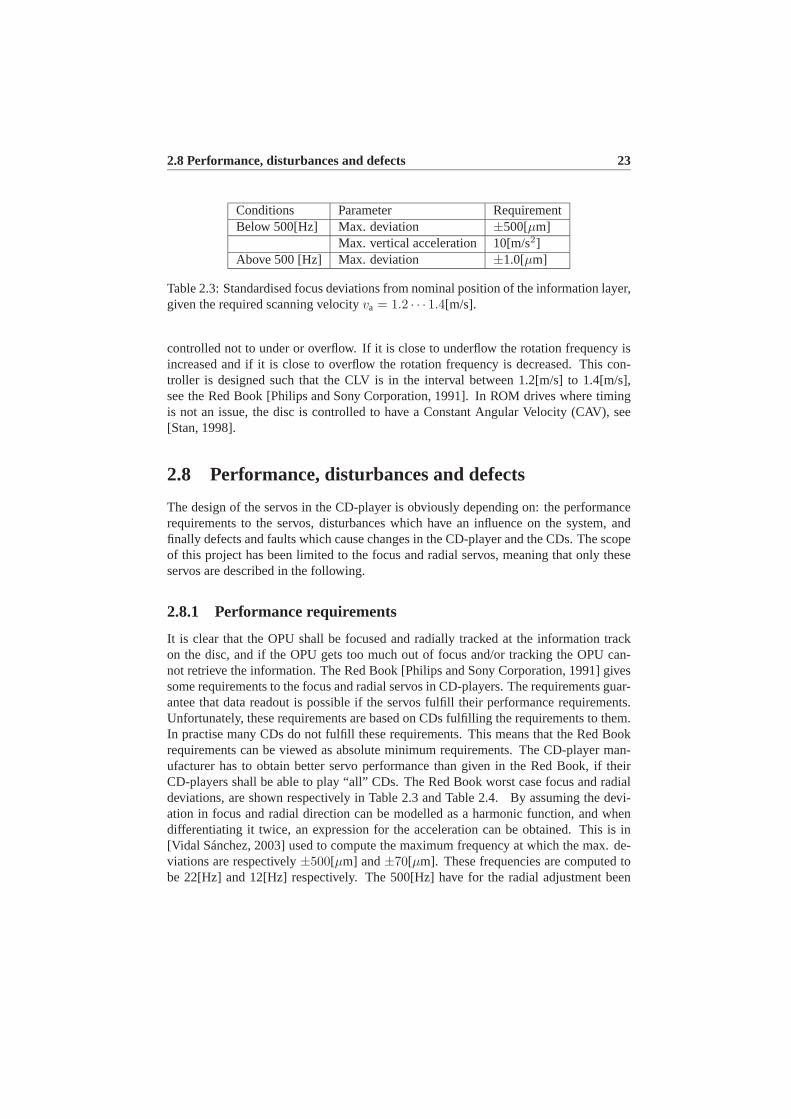
2.8 Performance, disturbances and defects 23
Conditions Parameter RequirementBelow 500[Hz] Max. deviation ±500[µm]
Max. vertical acceleration 10[m/s2]Above 500 [Hz] Max. deviation ±1.0[µm]
Table 2.3: Standardised focus deviations from nominal position of the information layer,given the required scanning velocityva = 1.2 · · · 1.4[m/s].
controlled not to under or overflow. If it is close to underflow the rotation frequency isincreased and if it is close to overflow the rotation frequency is decreased. This con-troller is designed such that the CLV is in the interval between 1.2[m/s] to 1.4[m/s],see the Red Book [Philips and Sony Corporation, 1991]. In ROM drives where timingis not an issue, the disc is controlled to have a Constant Angular Velocity (CAV), see[Stan, 1998].
2.8 Performance, disturbances and defects
The design of the servos in the CD-player is obviously depending on: the performancerequirements to the servos, disturbances which have an influence on the system, andfinally defects and faults which cause changes in the CD-player and the CDs. The scopeof this project has been limited to the focus and radial servos, meaning that only theseservos are described in the following.
2.8.1 Performance requirements
It is clear that the OPU shall be focused and radially tracked at the information trackon the disc, and if the OPU gets too much out of focus and/or tracking the OPU can-not retrieve the information. The Red Book [Philips and Sony Corporation, 1991] givessome requirements to the focus and radial servos in CD-players. The requirements guar-antee that data readout is possible if the servos fulfill their performance requirements.Unfortunately, these requirements are based on CDs fulfilling the requirements to them.In practise many CDs do not fulfill these requirements. This means that the Red Bookrequirements can be viewed as absolute minimum requirements. The CD-player man-ufacturer has to obtain better servo performance than given in the Red Book, if theirCD-players shall be able to play “all” CDs. The Red Book worst case focus and radialdeviations, are shown respectively in Table 2.3 and Table 2.4. By assuming the devi-ation in focus and radial direction can be modelled as a harmonic function, and whendifferentiating it twice, an expression for the acceleration can be obtained. This is in[Vidal Sánchez, 2003] used to compute the maximum frequency at which the max. de-viations are respectively±500[µm] and±70[µm]. These frequencies are computed tobe 22[Hz] and 12[Hz] respectively. The 500[Hz] have for the radial adjustment been
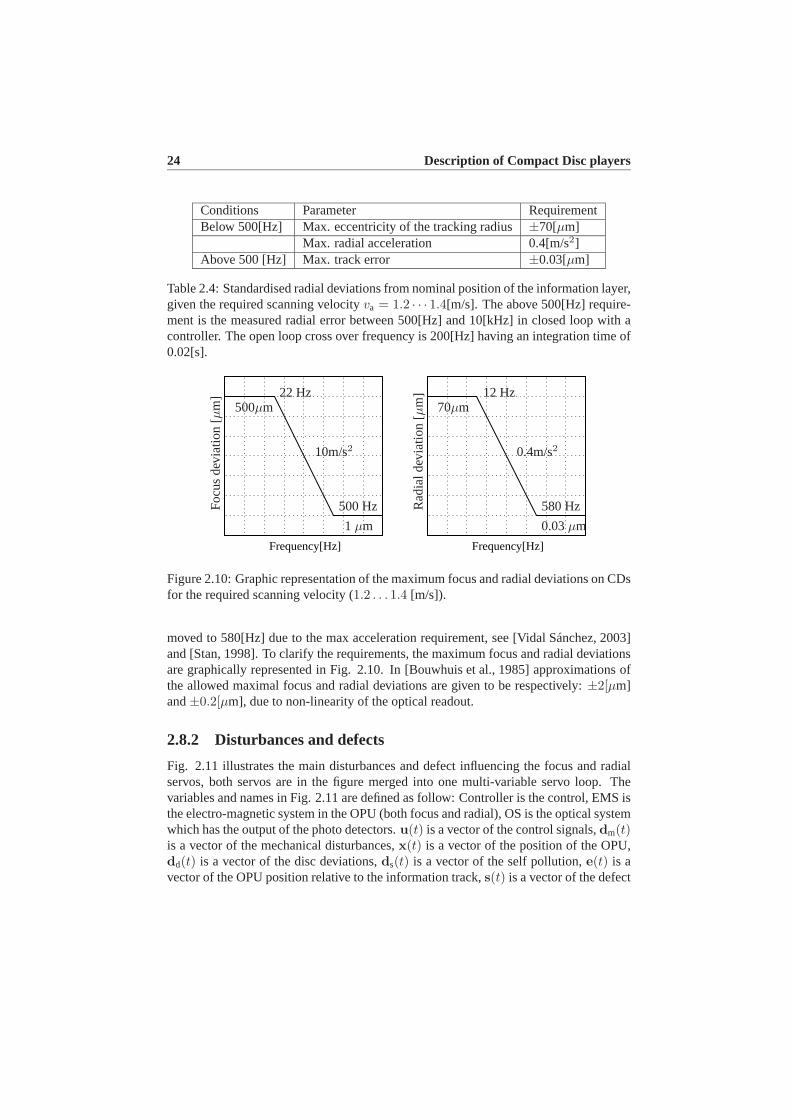
24 Description of Compact Disc players
Conditions Parameter RequirementBelow 500[Hz] Max. eccentricity of the tracking radius±70[µm]
Max. radial acceleration 0.4[m/s2]Above 500 [Hz] Max. track error ±0.03[µm]
Table 2.4: Standardised radial deviations from nominal position of the information layer,given the required scanning velocityva = 1.2 · · · 1.4[m/s]. The above 500[Hz] require-ment is the measured radial error between 500[Hz] and 10[kHz] in closed loop with acontroller. The open loop cross over frequency is 200[Hz] having an integration time of0.02[s].
Frequency[Hz] Frequency[Hz]
Foc
usde
viat
ion
[µm
] 22 Hz500µm
10m/s2
500 Hz
1 µm
Rad
iald
evia
tion
[µm
] 12 Hz70µm
0.4m/s2
580 Hz
0.03µm
Figure 2.10: Graphic representation of the maximum focus and radial deviations on CDsfor the required scanning velocity (1.2 . . . 1.4 [m/s]).
moved to 580[Hz] due to the max acceleration requirement, see [Vidal Sánchez, 2003]and [Stan, 1998]. To clarify the requirements, the maximum focus and radial deviationsare graphically represented in Fig. 2.10. In [Bouwhuis et al., 1985] approximations ofthe allowed maximal focus and radial deviations are given to be respectively:±2[µm]and±0.2[µm], due to non-linearity of the optical readout.
2.8.2 Disturbances and defects
Fig. 2.11 illustrates the main disturbances and defect influencing the focus and radialservos, both servos are in the figure merged into one multi-variable servo loop. Thevariables and names in Fig. 2.11 are defined as follow: Controller is the control, EMS isthe electro-magnetic system in the OPU (both focus and radial), OS is the optical systemwhich has the output of the photo detectors.u(t) is a vector of the control signals,dm(t)is a vector of the mechanical disturbances,x(t) is a vector of the position of the OPU,dd(t) is a vector of the disc deviations,ds(t) is a vector of the self pollution,e(t) is avector of the OPU position relative to the information track,s(t) is a vector of the defect
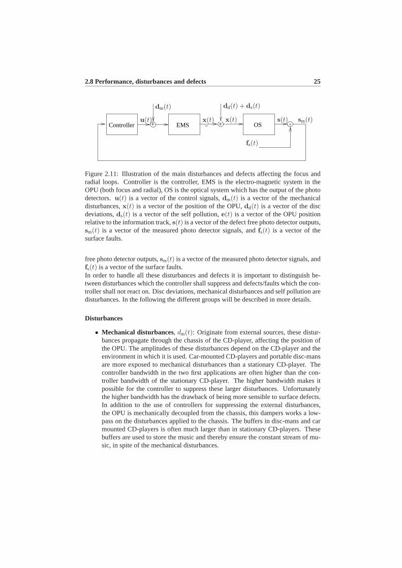
2.8 Performance, disturbances and defects 25
OS−Controller EMS+ +u(t)
dm(t)
x(t)
dd(t) + ds(t)
x(t) s(t) sm(t)
fs(t)
Figure 2.11: Illustration of the main disturbances and defects affecting the focus andradial loops. Controller is the controller, EMS is the electro-magnetic system in theOPU (both focus and radial), OS is the optical system which has the output of the photodetectors.u(t) is a vector of the control signals,dm(t) is a vector of the mechanicaldisturbances,x(t) is a vector of the position of the OPU,dd(t) is a vector of the discdeviations,ds(t) is a vector of the self pollution,e(t) is a vector of the OPU positionrelative to the information track,s(t) is a vector of the defect free photo detector outputs,sm(t) is a vector of the measured photo detector signals, andfs(t) is a vector of thesurface faults.
free photo detector outputs,sm(t) is a vector of the measured photo detector signals, andfs(t) is a vector of the surface faults.In order to handle all these disturbances and defects it is important to distinguish be-tween disturbances which the controller shall suppress and defects/faults which the con-troller shall not react on. Disc deviations, mechanical disturbances and self pollution aredisturbances. In the following the different groups will be described in more details.
Disturbances
• Mechanical disturbances, dm(t): Originate from external sources, these distur-bances propagate through the chassis of the CD-player, affecting the position ofthe OPU. The amplitudes of these disturbances depend on the CD-player and theenvironment in which it is used. Car-mounted CD-players and portable disc-mansare more exposed to mechanical disturbances than a stationary CD-player. Thecontroller bandwidth in the two first applications are often higher than the con-troller bandwidth of the stationary CD-player. The higher bandwidth makes itpossible for the controller to suppress these larger disturbances. Unfortunatelythe higher bandwidth has the drawback of being more sensible to surface defects.In addition to the use of controllers for suppressing the external disturbances,the OPU is mechanically decoupled from the chassis, this dampers works a low-pass on the disturbances applied to the chassis. The buffers in disc-mans and carmounted CD-players is often much larger than in stationary CD-players. Thesebuffers are used to store the music and thereby ensure the constant stream of mu-sic, in spite of the mechanical disturbances.

26 Description of Compact Disc players
• Self pollution, ds(t): is caused by internal factors inside the CD-player, e.g. crosscouplings between focus and radial actuators, sledge and radial, and disc servo tothe other loops.
• Disc deviations, dd(t): This group is due to deformations of the CD or CD-playerin a way that cause position deviations of the information track. Some examplesare: disc warp, skew discs and eccentric discs. These disturbances result in peri-odic disturbance with a natural frequency equal the rotation frequency of the disc.The maximal amplitudes, see [Philips and Sony Corporation, 1991], are given bythe specifications in Tables 2.3 and 2.4. In addition inaccuracies in the mechanicalclamping of the CD in the CD-player can also cause deviations in the position ofthe information track.
Defects
• Surface defects, fs(t): The remaining challenges in control of CD-players arein this group. These surface defects change the read-out from the disc by im-ply changes on the disc surface and these surface defects are: scratches, finger-prints, dust and other surface debris, coating defects, birefringence due to moldingproblems, air bubbles, thickness irregularities, etc. The three defects: scratches,fingerprints and dust are of interest in the remainder of this thesis.
2.8.3 Surface faults
Scratches, fingerprints and dust are following denoted surface faults. The surface faultsinfluence the photo detectors signal in such a way that the generated feedback signalalso contains a faulty part due to the surface faults. During a surface fault the controllerswill base their computation of the control signalu(t) on the feedback signal containinga faulty component due to the surface fault. The controllers can force the OPU out offocus and / or radial tracking due to this fault feedback signal component. Almost allCD-players have implemented some kind of fault handling, it is often implemented bydetecting the faults based on a fast drop in detected light energy. During a surface faultthe feedback signals are not entirely reliable, this means that a simple way to handlethem is to sample with a low enough sample frequency such that the surface fault canbe placed between two samples, in practice this i done by decreasing the controllerbandwidth during the occurrence of the surface fault. When the fault is detected thecontroller bandwidth is decreased, in practise the feedback signal is often fixed at zero,which introduces some unwanted controller reactions to this step in the feedback signal.At the detection of the end of the fault the bandwidth is put back to the normal, see[Philips, 1994], [Andersen et al., 2001] and [Vidal et al., 2001b]. However, this switchback to normal control does often cause more severe problems than the handling ofthe surface faults. The handling of both surface faults and mechanical disturbances isclearly conflicting, since the handling of surface fault requries a low bandwidth which

2.9 Proposed feature based control strategy 27
is in conflict with the requirement of a high bandwidth for handling disturbances. Thefact that disturbances and surface faults are non separable in time domain and frequencydomain also increase the complexity of solving this control problem. The error codingdescribed in the Red Book allows faults of a size up to 2.5 [mm], and the used handlingstrategies do not handle anything near to that size. The handling of these surface faultsis of the interest in the remainder of this thesis.
2.8.4 Playability
The Red Book defines the maximal physical tolerances of CDs, as well as gives speci-fications to the CD-players. These specifications ensure compatibility between the CDsand the CD-players. This means that it can be said that the playability is ensured as longas the Red Book requirements are fulfilled. In [Vidal Sánchez, 2003] a more broaderdefinition is given as
Definition 2.1 (Playability) the ability to reproduce the information from non-idealdiscs in non-ideal circumstances.
[Vidal Sánchez, 2003] also divides the playability constraints into three major groups:HF signal, data channel and servo. This Ph.D work focus on improvement of the playa-bility by addressing the servo part. The servo part of the playability problem can againbe divided into the disturbances and faults described in Section 2.8.2. The remainder ofthe thesis is focused on improving the playability regarding surface faults without low-ering the playability towards the other servo issues. The work will especially be focusedon the handling of surface faults originating from the use of the CDs, such as scratchesand fingerprints, and not surface faults originating from the production of the CDs likeblack or white dots.
2.9 Proposed feature based control strategy
In order to improve the playability of discs with surface faults without lowering theplayability of other servo issues, a fault tolerant control strategy seems to be a wellsuited choice. This is supported by the work in [Vidal Sánchez, 2003]. It might also bea good idea to use a joint time/frequency analysis to extract features used to detect andhandle the surface faults. The general structure of the suggested strategy, called featurebased control, is illustrated in Fig. 2.12.The CD-player feeds the photo detectors signals to the residual generator, which com-putes fault residuals. These residuals and the distance measurements are following usedto locate the faults and to extract features of the fault which can be used to accommo-date the controller to handle the fault. The fault is first located in time, (also called faultdetection), followed by the extraction of the useful features. Due to the small distance
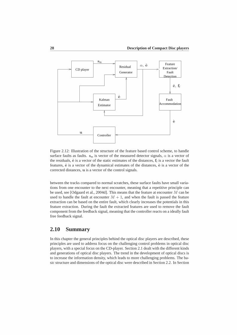
28 Description of Compact Disc players
Generator
Residual
AccommodationFault
FeatureExtraction/
FaultDetection
Kalman
Estimator
CD player
Controller
smα, e
e
u
e, ff
e
Figure 2.12: Illustration of the structure of the feature based control scheme, to handlesurface faults as faults.sm is vector of the measured detector signals,α is a vector ofthe residuals,e is a vector of the static estimates of the distances,ff is a vector the faultfeatures,e is a vector of the dynamical estimates of the distances,e is a vector of thecorrected distances,u is a vector of the control signals.
between the tracks compared to normal scratches, these surface faults have small varia-tions from one encounter to the next encounter, meaning that a repetitive principle canbe used, see [Odgaard et al., 2004d]. This means that the feature at encounterM can beused to handle the fault at encounterM + 1, and when the fault is passed the featureextraction can be based on the entire fault, which clearly increases the potentials in thisfeature extraction. During the fault the extracted features are used to remove the faultcomponent from the feedback signal, meaning that the controller reacts on a ideally faultfree feedback signal.
2.10 Summary
In this chapter the general principles behind the optical disc players are described, theseprinciples are used to address focus on the challenging control problems in optical discplayers, with a special focus on the CD-player. Section 2.1 dealt with the different kindsand generations of optical disc players. The trend in the development of optical discs isto increase the information density, which leads to more challenging problems. The ba-sic structure and dimensions of the optical disc were described in Section 2.2. In Section

2.10 Summary 29
2.3 the general structure of the optical disc players was revealed. Some required basicoptical principles are described in Section 2.4, where these are used to reveal some ofoptical differences in the different generations of optical discs. This lead to a descrip-tion of the optical pick-up, see Section 2.5. Due to the lack of physical contact betweenthe optical pick-up and the information track on the optical disc, control is needed tofocus and radially track the optical pick-up at the information track on the optical disc.Section 2.6 described the indirect measurement of the feedback signals used to posi-tion the optical pick-up - These feedback signals are used in servo loops to positioningthe optical pick-up. The servo loops were the topic of Section 2.7. These servos arerequired to fulfill some performance requirements. The servo shall also suppress distur-bances such as mechanical disturbances and disc deviations, and handle surface faultssuch as scratches by not reacting to these, see Section 2.8. These requirements are highlyconflicting since disturbances and faults partly coexist in the same frequency and timeregion. A way to handle this control problem is to address it by a feature based faulttolerant control scheme. The control scheme is introduced in Section 2.9.

Chapter 3
Model of a Compact Disc Player
This chapter deals with the modelling of focus and radial actuators and sensors in theCD-player, these models are derived with the purpose of designing focus and radialcontrollers in a given CD-player. Normally these controllers in the servos are designedbased on dynamical models of the mechanical and electro-magnetic parts of the CD-players. The optics are normally modelled by a simple linear static model, which issufficient for the design of nominal controllers for the focus and radial servos. However,in the case of fault detection, there are some optical cross-couplings which makes earlydetection of the surface faults impossible if an optical model is not used.A large effort is put in modelling and identification of the mechanical and electro-magnetic parts of CD-players. [Bouwhuis et al., 1985] focuses on the modelling of theseparts of the system and [Vidal et al., 2001c] describes a simple method to perform openloop system identification. Both [Yeh and Pan, 2000] and [Dettori, 2001] perform somework on modelling the cross-couplings in the mechanical and electro-magnetic partsbetween focus and radial loop. Regarding the optical part of the system the present con-trol strategies are based on simple linear models which do not concern the optical crosscoupling [Bouwhuis et al., 1985] and [Stan, 1998], although some work has been doneregarding the optical model. [Yeh and Pan, 2000] has some considerations about the op-tical cross-couplings. [Vidal et al., 2001b] and [Vidal et al., 2001a] deal with models ofthe optical signal of focus distance without consideration about the cross coupling withthe radial loop. This model is used for detection of surface faults on the disc. The prin-ciple behind the optical pick-up applied in this work is the single Foucault three beamprinciple, which is described in [Stan, 1998], [Bouwhuis et al., 1985]. Based on theseprinciples and measurements on a CD-player test setup, a model of a three beam singleFoucault optical detector system is made. This model maps from focus and radial dis-tances to focus sensors and radial sensor signals. The model includes the cross-couplingsbetween focus and radial loops. This optical model is followed by a model of the surfacefaults.The used experimental test setup is described in Section 3.1. In Section 3.2 a model
31

32 Model of a Compact Disc Player
structure of the focus and radial servos is given, in Section 3.3 the mechanical andelectro-magnetic model is derived. This leads to the main novel contributions in thischapter: the optical model in Section 3.4 and the surface fault model in Section 3.5.
3.1 Experimental test setup
Some of the results of this thesis were tested on an experimental test setup which will bedescribed in this section, with a focus on the possibilities and limitations this experimen-tal test system gives. A stereo music system with a CD-drive is used as main part of theexperimental test system. The stereo system has implemented internal focus and radialPID controllers. These controllers are digitally implemented with a fixed size and struc-ture. As a consequence it is only possible to change the parameters in these controllers.These limitations can be bypassed by using a PC-based experimental setup, as illustratedin Fig. 3.1. A photo of the experimental test setup is shown in Fig. 3.2. This experimen-tal test setup is the same as used in [Vidal Sánchez, 2003], which again is based on aprevious design documented in [Vidal et al., 1998] and [Andersen and Karlsson, 2000].The original CD-drive is separated from the stereo music system, but still connectedthrough the communication link such that the music stereo system can be operatedas normal. The built-in PID controllers receive as inputs the four detector signals:D1, D2, S1, S2. The control signals computed by these PID controllers,uf andur
conducted through the PC-controlled switches to the CD-drive, which closes the controlloops. An alternative to this setup is that the focus and radial positions are controlledby the controllers in the PC. The photo diode signals are fed through the PCI 9118-DGI/O-card to the PC. The photo diode signals are in this process amplified, low-pass fil-tered and discretised by the I/O-card. In the PC two control signals are computed andpassed following through an attenuator stage. The PC also changes the PC-controlledswitches so the CD-drive can be controlled by the PC instead of the built-in controllers.In addition the control signals computed by the internal PID controllers are also sampledby the PC.In the following the relevant specifications of the experimental test setup are listed. Aconsequence of the relative old PC and I/O-card is the trade-off regarding the samplefrequency and bandwidth of the anti-aliasing filter. Even though these are higher inindustrial players, these are chosen due to computational limitations of the PC and I/O-card. However, the listed data are acceptable and usable trade-offs.
• Amplifier gain: Photo diode gain: 60 [dB], Control signal measurement gain: 40[dB].
• Anti-aliasing filter: First order low pass filter with a 8 [kHz] bandwidth.
• Attenuation factor for control output: -54 [dB].
• PCI 9118-DG I/O-card: 8 12 bit±5 [V] analog inputs with on-chip sample-and-hold. 2 12 bit±10 [V] analog outputs. 35 [kHz] sample frequency for each

3.1 Experimental test setup 33
Developedhardware
PC
Stereo music system
LinkCommunication
CD−Drive
Radial PID
Focus PID
Attenuator Amplifier
FilterLowpass
PCI 9118−DG I/O card
Ready
Software
Control
CD−Player
D1,D2, S1, S2
uf ur
Figure 3.1: Overview of the experimental setup. The CD-drive of the stereo system isconnected through the developed hardware to a PC. The focus and radial position can becontrolled by either the internal PID controllers or by controllers implemented in the PC.One should notice that it is possible to control one position with the internal controllerand the other position with the external controller.
channel. Direct Memory Access (DMA) data transfer.
• Personal Computer: AMD Athlon PC 1100 MHz with Dos 6.1 operating systeminstalled and C-compiler.
The amplifier is the most critical part of the experimental setup. The OPU generatescurrent signals below 12 [µA] which can not be sampled by the I/O-card. In additionsignals with such a low signal power are very sensitive to measurement noises. Measure-ment noises is a problem due to a long wire between the OPU and hardware. Amplifiersare used to convert these signals to voltages in the range of the I/O-card.

34 Model of a Compact Disc Player
Figure 3.2: Photo of the experimental test setup.
CD-drive The CD-drive used in the experimental test setup is based on the followingprinciples: A holographic optics arrangement, which implements the focus and radialoptical detectors. The used focus detector principle is the single Foucault principle, andthe used radial detector principle is the Three-beam method. The optics are positionedusing a 2-axis device mounted on a sledge.These detector and actuator principles are described in this chapter 2, and modelled laterin this chapter.
Limitations An on-the-fly switch from the internal to the external controller is onlypossible in the focus loop. At the time of switching, any difference between the internaland external controller’s output introduces a step on the control signals applied to theactuators. The focus loop accepts large errors (±6[µm]) before loosing focus and hasshown in practice to be robust towards these steps. The radial loop on the other hand hasshown to be much more sensitive towards these steps. This is a consequence of the factthat a change larger than 0.8µm results in a jump to the next track. The built-in logic inthe stereo music system tries to correct that by jumping back to the previous revolution.However, this is not possible, since the radial position is controlled by the PC. The built-in logic will as a result generate a failure which stops the CD-player immediately. Away to work-around this problem is to implement the radial controller when the stereomusic system is in test mode, where no actions are taken in case the presence of jumpin tracks. It has the drawback that the sledge controller is not applied, meaning that the
3.2 Model structure 35
radial controller can work only in a few seconds before it reaches the saturation limits.The low-budget PCI9118-DG I/O-card does also introduce some limitations in the testsystem. It is designed to be used in applications where data is sampled in a row andturn-around delay is not critical. In closed-loop systems these delays lead to instabilityand severe limitations in the performance. These delays should as a consequence beavoided. The used software on the PC was created in a way such that the delay islimited to two sample periods. A better alternative is used in [Dettori, 2001] where theexperimental setup is based on dSpace, which offers a powerful design tool for control,but at a high price. In [Dettori, 2001] a hardware-software based solution where theradial controller can be changed on-the-fly with out the limitations of the experimentalsetup of the present Ph.D work.
3.2 Model structure
The lack of physical contact between the OPU and the information track on the CD,results in the need of focusing and radial tracking of the OPU. These are performedby the use of two servo loops, where the physical adjustments are performed by the2-axis device, which enables positions adjustments in both the focus and radial direc-tion. A number of alternative implementations of this devices are also used. Only the2-axis device used in the test setup, in this work, will be described. This 2-axis deviceuses two linear electro-magnetic actuators to adjust the OPU in the focus and radialdirection. These actuators are by design placed orthogonal to each other, resulting intheory in non-electro-magnetic cross-couplings between the two actuators. The OPUis suspended on four parallel arms, as illustrated in Fig. 3.4. The actuators enable theadjustments of the OPU, but are also necessary to measure the focus and radial distancesin order to adjust them to be zero. By the use of smart optics, the OPU generates someindirect measurements of these distances. The indirect measurements can be performedin a number of ways. In this work the single Foucault method is used to measure thefocus distance and the three beam principle is used to measure the radial distances. Themain problem to solve in this Ph.D project is to handle surface faults that are impossibleto handle by normally used methods. It is anticipated that the use of a model of surfacefaults would make this possible. This gives the third model block, enabling an illustra-tion of the overall model structure. This model structure is illustrated in Fig. 3.3. Thethree sub-models are the electro-magnetic-mechanical model, the optical model and thesurface fault model.
3.3 Electro-magnetic-mechanical model
The focus and radial actuators are in principle identical, meaning they can be describedwith the same model. As a consequence only the focus actuator will be described inthe following. The electro-magnetic part of the OPU is again composed by two parts, a

36 Model of a Compact Disc Player
SF−EMS OS++u(t)
dm(t)
x(t)
dm(t) + dd(t) + ds(t)
xcd(t) s(t) sm(t)
Figure 3.3: Illustration of general model structure of the combined focus and radialmodel. EMS is a model of the electro-magnetic-mechanical system in the OPU, OS isthe optical model which has the output of the photo detectors, and SF is a model of thesurface faults.u(t) is a vector of the control signals,dm(t) is a vector of mechanicaldisturbances,x(t) is a vector of the positions of the OPU,dd(t) is a vector of the discdeviations,ds(t) is a vector of the self pollutions,xcd(t) is a vector of the OPU positionsrelative to the information track,s(t) is a vector of the fault free photo detector outputs,sm(t) is a vector of the measured photo detector signals, andfs(t) is a vector of thesurface faults.
Top viewSide view
ef+
ef−
er+
er−
LensLens
Radial CoilRadial Coil Focus CoilFocus Coil
Radial SpringRadial Spring
Focus SpringFocus Spring
Figure 3.4: Illustration of 2-axis device suspended on four parallel arms, where twolinear electro-magnetic actuators are used for the focus and radial adjustments.
driver part and a mechanical part. These two parts are described in more details in thefollowing two subsections, ending up with a transfer function for the electro-magneticmodel.
3.3.1 Electro-magnetic part
The driver performs the conversion from the applied control voltageu(t) to the forceacting on the mechanical part of the actuatorF (t). The active part in this actuator is thecoil which is driven by a current. The power driver convertsu(t) to the currenti(t). Thepower driver is modelled by a constant gainKpd and results in a different voltage acrossthe linear electro-magnetic actuator,ucoil(t). The power driver is not physically placedin the OPU, but is considered to be a part of it, and is as a consequence a part of thedriver part. A sketch of the driver part is drawn in Fig. 3.5.

3.3 Electro-magnetic-mechanical model 37
+
−
+
−Driver
Poweru(t)ucoil(t)
R L
em(t)i(t)F (t)
Figure 3.5: Sketch of the driver part of the model. The applied control voltageu(t) isconverted into a currenti(t). The current runs through the coil and in the magnetic fieldthis results in a forceF (t). ucoil(t) is the voltage over the coil,em(t) is the inducedvoltage,R is the resistance in the coils, andL is the inductance in the coils.
This linear electro-magnetic actuator behaves like a direct-current (dc) motor for re-stricted displacements, which is the case of the normal use of the actuator. The dc motorequivalent electrical diagram is shown in Fig. 3.5. The equivalent is composed by a re-sistanceR, an inductanceL and the induced voltage sourceem(t). By using Kirchhoff’svoltage lawucoil(t) can be computed
u(t) · Kpd = ucoil(t) = R · i(t) + L · i(t) + em(t). (3.1)
The induced voltageem(t) is a result of the coil movements relative to the magneticfield. em(t) is described by the following equation
em(t) = (x(t) × B) · l, (3.2)
wherex(t) is the velocity of the coil in the magnetic field,B is the flux density of themagnetic field andl is the length of the moving coil. In practice this cross product canbe replaced by a scalar product since the three vectors are mutually orthogonal. Thisresults in a simplification of (3.2)
em(t) = B · l · x(t). (3.3)
i(t) can be calculated by substitutingem from (3.3) into (3.1), followed by an isolationof i(t)
i(t) =u(t) · Kpd − B · l · x(t)
R + L · s . (3.4)
A different physical law governs the electrical induced force,F (t). The conductor isassumed to be fixed for simplicity. The current through the conductor in interactionswith the magnetic field generates a force on the conductor. It can be described by thefollowing equation
F(t) = i(t) · (B × l). (3.5)

38 Model of a Compact Disc Player
Again the vectors are mutually orthogonal, meaning that (3.5) can be simplified to
F (t) = B · i(t) · l. (3.6)
By assuming the system to be linear a transfer function in the laplace domain can bestated, by laplace transform (3.4) into (3.6).F (s) can now be calculated by substitutingi(s) in the two laplace transformed equations.
F (s) = B · l · u(s) · Kpd − B · l · s · x(s)R + l · s . (3.7)
3.3.2 Mechanical part
The force generated by the electro-magnetic part,F (t) is applied to the OPU of themassm. A simple model of the mechanical part is suggested in [Bouwhuis et al., 1985].Assume the effects from friction, elasticity, etc. to be neglectable, then this system willact like a double integrator, described by Newton’s second law,F = mx, wherex is theacceleration of the OPU. The position follows by integrating the acceleration twice. Themechanical parts are assumed to be linear, and it is whereby possible to state the forceto position transfer function in the Laplace domain given as
x(s)F (s)
=1
m · s2. (3.8)
In principles all optical disc players have mechanical parts which can be modelled asbeing double integrators, see [Bouwhuis et al., 1985]. However, the OPU is not floatingas assumed in (3.8), it is suspended on leaf-springs. Taking the these leaf-springs intoaccount the mechanical part can be modelled by a mass-spring-damper model, as illus-trated in Fig. 3.6.m is the mass of the moving OPU,x(s) is the displacement,b andk isrespectively the damping and spring constant, andF (s) is the applied force. This givesa new transfer function
x(s)F (s)
=1
m · s2 + b · s + k. (3.9)
This model structure is used in this work, even though a more precise model would be tointroduce an parasite mass-spring-damper system. The pole which the additional mass-spring-damper introduces is placed at a high frequency where this work does not need aprecise model. This means that the transfer function in (3.9) is used as a model of themechanical part of the system.
3.3.3 General electro-magnetic model
This model can be achieved if the models of the mechanical part and the electro-magnetic part are merged. In order to achieve a transfer function in the Laplace domain,the electro-magnetic part of this model is assumed to be linear. The transfer function

3.3 Electro-magnetic-mechanical model 39
F (t)
x(t)
m
spring,k
damper,b
mass
Figure 3.6: Free body diagram of the mass-spring-damper system.
from the applied focus control voltageuf(s) to the focus distanceef(s) can be found bysubstituting the force from (3.7) into (3.9), and followed by an isolation of the requiredvariables. The transfer function is derived as
ef(s)uf(s)
= Kpd ·B·lm·R
LR · s · (s2 + b
m · s + km
)+
(s2 +
((B·l)2m·R + b
m
)· s + k
m
) . (3.10)
The radial transfer function fromur(s) to the radial distanceer(s), can be derived inthe same way. The test-setup used is the same as used in [Vidal Sánchez, 2003]. Thepole related to the inductanceL is in [Vidal Sánchez, 2003] approximated to above10[kHz] for both the focus and radial actuators, which are above the typical closedloop bandwidth of both the focus and radial loops in CD-players, since the interval oftypical closed loop bandwidth is 0.5-2[kHz], (see for example [Steinbuch et al., 1994],[Yokoyama et al., 1994], [Chait et al., 1994], [Huang et al., 1999], [Moon et al., 1996]and [Dettori et al., 1999]). This means that the inductor can be neglected.
Model adapted to the test-setup drive By neglecting the pole due to the inductance,both the focus and radial actuators can be described with second order transfer functions.The focus transfer function is
ef(s)uf(s)
= Kpd,f ·Bf ·lfRf ·mf
s2 +(
bfmf
+ (Bf ·lf)2
mf ·Rf
)· s + kf
mf
, (3.11)
where:Kpd,f is the focus power driver gain,Bf is the magnetic flux density in the focusactuator,lf is the length of the moving coil in the focus actuator,Rf is the resistance in

40 Model of a Compact Disc Player
the focus actuator,mf is the mass which is moved by the focus actuator,kf is the springconstant of the focus actuator andbf is the damper constant of the focus actuator. Theradial transfer function is
er(s)ur(s)
= Kpd,r ·Br·lrRr·mr
s2 +(
brmr
+ (Br·lr)2
mr·Rr
)· s + kr
mr
, (3.12)
where:Kpd,r is the radial power driver gain,Br is the magnetic flux density in the radialactuator,lr is the length of the moving coil in the radial actuator,Rr is the resistance inthe radial actuator,mr is the mass which is moved by the radial actuator,kr is the springconstant of the radial actuator andbr is the damper constant of the radial actuator. In[Vidal Sánchez, 2003] these model parameters are estimated, and since Vidal performedthis parameters estimation on the same test setup as used in this work, the parametersestimated in [Vidal Sánchez, 2003] are used. The models can be seen in Appendix A.
3.4 Optical model
The often used model of the optical systems of the CD-player is a simple model,assuming the focus and radial distances to be linearly dependent on the differenceon their respectively photo detectors, see [Bouwhuis et al., 1985], [Stan, 1998] and[Pohlmann, 1992]. Doing so one neglects the optical cross-coupling and the non-linearbehaviour of the optical system. This optical cross-coupling is not so important in theestimations of the focus and radial distances. It is much more important in the detectionof surface faults. The normal strategy is to detect fast changes in the received energy, see[Andersen et al., 2001] and [Philips, 1994]. The amount of received energy can approx-imated by the sum of the two focus detectors or the two radial detectors. Unfortunately,the optical cross-coupling has a clear contribution to these sum signals, meaning that thefocus sum depends on the radial distance, and the radial sum depends on the focus dis-tance. This indicates that a model of the optical system mapping from focus and radialdistances to the four detector signal would be of good use.The modelling of CD-players have been focused on the electro-magnetic parts ofthe CD-player, although some work has been done regarding the optical model.[Yeh and Pan, 2000] have some considerations about the optical cross-couplings.[Vidal et al., 2001b] and [Vidal et al., 2001a] deal with models of the optical signal ofthe focus error without consideration about the cross-couplings with the radial loop. Thismodel is used for detection of surface faults on the disc. In DVD-players [Filardi, 2003]and [Hnilicka et al., 2002] have modelled the focus and radial mappings without tak-ing any cross-couplings into account. Focus has been put on the optical model of theread-out process, see [Honguh, 2002] and [Kojima and Wakabayashi, 1997], which isnot the same as the modelling of the optical detectors, even though some similaritiesdo occur. The optical model of the CD-player used in this Ph.D project can be foundin [Odgaard et al., 2003c], which models a CD-player with three beam single Foucault
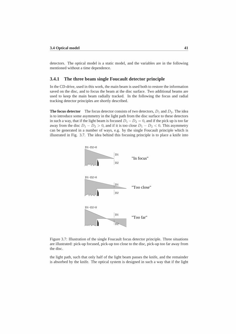
3.4 Optical model 41
detectors. The optical model is a static model, and the variables are in the followingmentioned without a time dependence.
3.4.1 The three beam single Foucault detector principle
In the CD-drive, used in this work, the main beam is used both to restore the informationsaved on the disc, and to focus the beam at the disc surface. Two additional beams areused to keep the main beam radially tracked. In the following the focus and radialtracking detector principles are shortly described.
The focus detector The focus detector consists of two detectors,D1 andD2. The ideais to introduce some asymmetry in the light path from the disc surface to these detectorsin such a way, that if the light beam is focusedD1−D2 = 0, and if the pick up is too faraway from the discD1 − D2 > 0, and if it is too closeD1 − D2 < 0. This asymmetrycan be generated in a number of ways, e.g. by the single Foucault principle which isillustrated in Fig. 3.7. The idea behind this focusing principle is to place a knife into
"In focus"
"Too far"
"Too close"
D1−D2=0
D1−D2<0
D1−D2>0
D2
D1
D2
D1
D1
D2
Figure 3.7: Illustration of the single Foucault focus detector principle. Three situationsare illustrated: pick-up focused, pick-up too close to the disc, pick-up too far away fromthe disc.
the light path, such that only half of the light beam passes the knife, and the remainderis absorbed by the knife. The optical system is designed in such a way that if the light

42 Model of a Compact Disc Player
Spread of the beam
0.5
light energyNormalised
1
diameterSpot
����������������������
����������������������
Figure 3.8: Illustration of the light intensity, and the approximation by assuming thelight source being a disc with the radius equal to the radius of the half-intensity level.
beam is focused on the disc it would also be focused on the detectors. In the cases wherethe pick-up is either too close to or too far away from the disc, the beam focus pointwould be either behind or in front of the detectors. The principle illustrated in Fig. 3.7is based on the assumption that the light source is point source. A better description ofthe source, however, is to use the energy distribution of the laser beam which is shapedlike a sinc function, see [Stan, 1998] and [Bouwhuis et al., 1985], as illustrated in Fig.3.8. This is simplified by assuming the light source being a disc with a radius equal tothe radius of the half-intensity level, and with a uniform light intensity.The disc shaped light source results in light being detected on bothD1 andD2 in almostall situations, but the principle is the same as illustrated in Fig. 3.7. The sign of thedifference betweenD1 andD2 is the same as in Fig. 3.7.
Radial detector Fig. 3.9 illustrates how the three beams, (main beam and the two sidebeamsS1 andS2), are placed relative to each other on the disc surface. The main spot isplaced in the middle of the track and the two others placed one to each side of the track,with a distance from their centre to the middle of the track calledak. If the pick-up islocated symmetrically over the track, the two side spots will cover equal areas of the
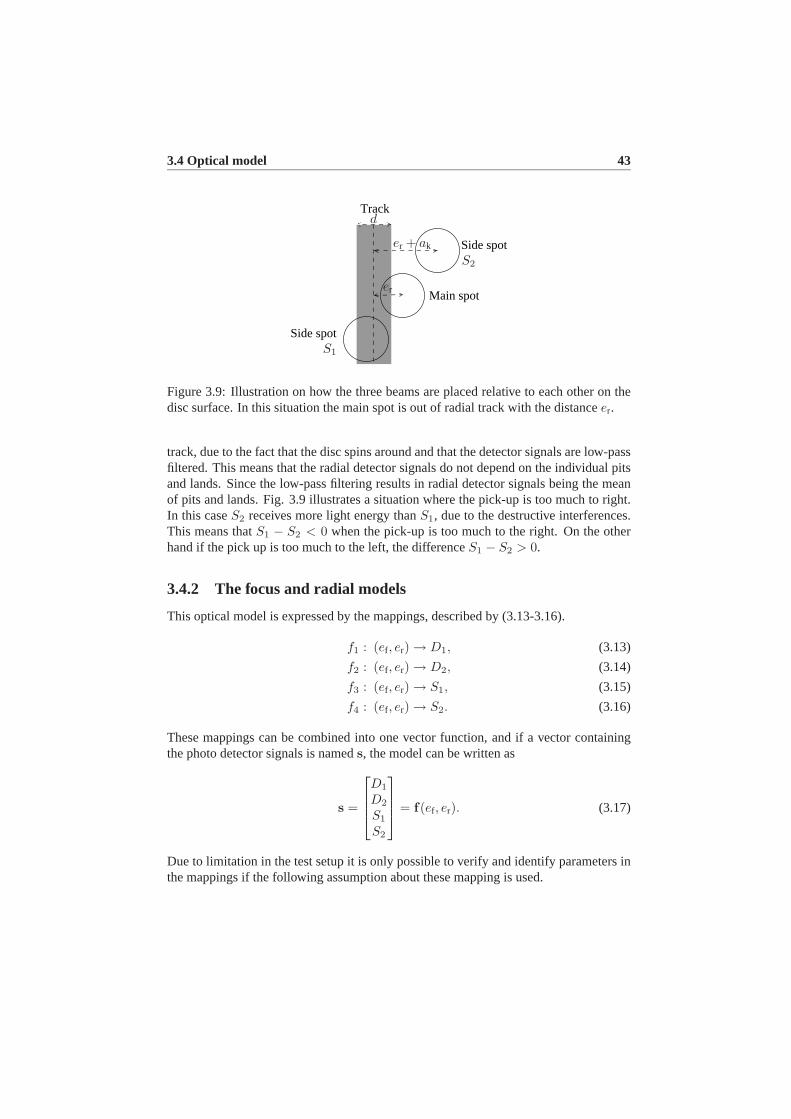
3.4 Optical model 43
Side spot
Side spot
Main spot
Track
S1
S2
er
er + ak
d
Figure 3.9: Illustration on how the three beams are placed relative to each other on thedisc surface. In this situation the main spot is out of radial track with the distanceer.
track, due to the fact that the disc spins around and that the detector signals are low-passfiltered. This means that the radial detector signals do not depend on the individual pitsand lands. Since the low-pass filtering results in radial detector signals being the meanof pits and lands. Fig. 3.9 illustrates a situation where the pick-up is too much to right.In this caseS2 receives more light energy thanS1, due to the destructive interferences.This means thatS1 − S2 < 0 when the pick-up is too much to the right. On the otherhand if the pick up is too much to the left, the differenceS1 − S2 > 0.
3.4.2 The focus and radial models
This optical model is expressed by the mappings, described by (3.13-3.16).
f1 : (ef , er) → D1, (3.13)
f2 : (ef , er) → D2, (3.14)
f3 : (ef , er) → S1, (3.15)
f4 : (ef , er) → S2. (3.16)
These mappings can be combined into one vector function, and if a vector containingthe photo detector signals is nameds, the model can be written as
s =
D1
D2
S1
S2
= f(ef , er). (3.17)
Due to limitation in the test setup it is only possible to verify and identify parameters inthe mappings if the following assumption about these mapping is used.

44 Model of a Compact Disc Player
fi(ef , er) ≈ hi(ef) · gi(er), (3.18)
where
i ∈ {1, 2, 3, 4}. (3.19)
This assumption means that the radii of the spots at the disc is constant, even though theradii of the spots depend onef . However, an increase in the actual area of the spot is notimportant for this model. The important thing is the ratio between the area of the spotcovering the track,Atrack, and the area of the part of the spot covering some of the areabetween the tracks,ACD. This ratio is almost constant. This means that influence ofef
ong(·) can be neglected as a consequence, see [Odgaard et al., 2003c].(3.18) can be interpreted as follows. Thegi(er) function computes the maximal detectedenergy for a given value ofer. Thehi(ef) computes how large a ratio of the reflectedenergy in the spot which is detected at the photo detectors. In the following expressionsfor thehi(ef) andgi(er) functions are derived.
The hi(ef) mappings will be derived in the following, starting withh1(ef) andh2(ef).These two mappings are related in the following way:
h1(ef) = h2(−ef), (3.20)
due to the linear movement of the focus point relative to the detectors. As a consequenceof (3.20) it is only needed to model one of these function,h1(ef) is modelled. This modelof how ef influences the diode signals, consists of two factors,h1(ef) = h
′1(ef) · η1(ef).
The first factor,h′1(ef), is due to the single Foucault principle. The light beam at the
detector would have some kind of half disc shape, due to the single Foucault principle.The radius of the half disc,r, increases linearly withef . Factor number two,η1(ef), isthe ratio of light energy detected at the detectors compared to the amount of light energyintended to be detected. The ratio decreases, since the detectors have to be relativelysmall due to the implementation and in order to minimise the noise received throughthe detectors. As a consequence the light beam covers more and more area outside thedetector asef increases.The modelling of the optical detectors can now be started with,h
′1(ef), the first factor in
the model. First all the lenses in the light path from light source to the disc surface aremerged into one lens,F . This simplification is illustrated in Fig. 3.10The distance from the lens to the disc surface and back to the lens again, is denotedlx:
lx = lx,0 − 2 · ef . (3.21)
The distance from the source to the lens,lu is:
lu = lu,0 + ef , (3.22)
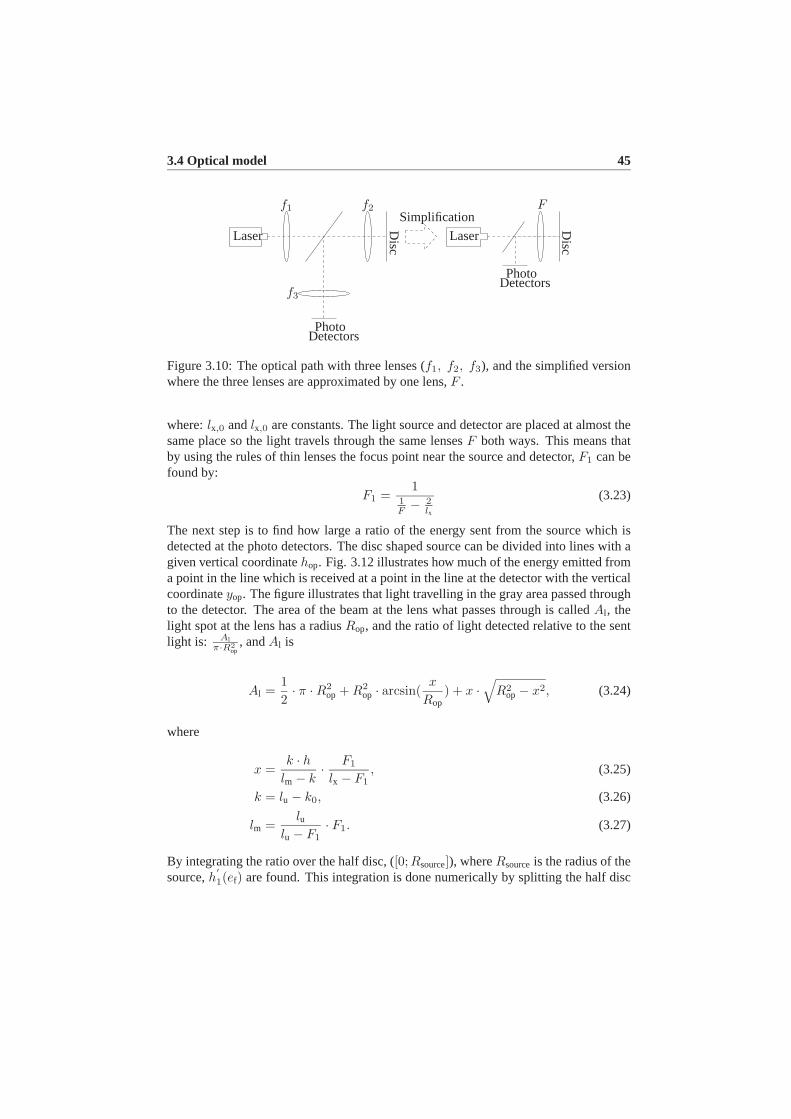
3.4 Optical model 45
f1 f2
f3
F
LaserLaser
Simplification
Disc
Disc
Photo
Photo
Detectors
Detectors
Figure 3.10: The optical path with three lenses (f1, f2, f3), and the simplified versionwhere the three lenses are approximated by one lens,F .
where:lx,0 andlx,0 are constants. The light source and detector are placed at almost thesame place so the light travels through the same lensesF both ways. This means thatby using the rules of thin lenses the focus point near the source and detector,F1 can befound by:
F1 =1
1F − 2
lx
(3.23)
The next step is to find how large a ratio of the energy sent from the source which isdetected at the photo detectors. The disc shaped source can be divided into lines with agiven vertical coordinatehop. Fig. 3.12 illustrates how much of the energy emitted froma point in the line which is received at a point in the line at the detector with the verticalcoordinateyop. The figure illustrates that light travelling in the gray area passed throughto the detector. The area of the beam at the lens what passes through is calledAl , thelight spot at the lens has a radiusRop, and the ratio of light detected relative to the sentlight is: Al
π·R2op
, andAl is
Al =12· π · R2
op + R2op · arcsin(
x
Rop) + x ·
√R2
op − x2, (3.24)
where
x =k · h
lm − k· F1
lx − F1, (3.25)
k = lu − k0, (3.26)
lm =lu
lu − F1· F1. (3.27)
By integrating the ratio over the half disc, ([0;Rsource]), whereRsourceis the radius of thesource,h
′1(ef) are found. This integration is done numerically by splitting the half disc

46 Model of a Compact Disc Player
123
i
4
Figure 3.11: Illustration on how the half disc approximated with rectangles with centresin xi and with the areasai.
up into approximation rectangles, and summing these. Fig. 3.11 is an illustration of theapproximation of the half disc with rectangles. The height of the rectangles,hop is givenby:
hop =Rsource
Pop, (3.28)
wherePop is the number of rectangles used for the approximation. These thin rectanglestend to a line asPop increases and thereby approximates the lines with a constant verticalcoordinatex. This method results inPop x values, i.e.xi, i ∈ [1, 2, · · · , Pop]. A relativearea function is defined as a function ofi, Arel(i). This relative area tells how large apart of the energy in the laser which is in a given vertical line. It is now possible toapproximate the integration over all the lines a given vertical constant, by summarisingall theAl(xi) multiplied withArel(i):
h′1(ef) =
12
+Pop∑0
R2op arcsin ( xi
Rop) + xi ·
√R2
op − x2i
π · R2op
· Arel(i). (3.29)
The modelling ofη1(ef) is basically to find the ratio of the light energy detected at thedetector relative to the energy intended to be detected. The shape of the detector isassumed to be a rectangle(bop × 2bop). Fig. 3.13 illustrates the three possible situationson how the reflected spot covers the detector. By inspecting Fig. 3.13, the expression ofη1(ef) can be found to be:
η1(ef) =
1 if a)12 ·πr(ef)
2−r(ef)2·(2θ1(ef)−sin(2·θ1(ef)))12 ·πr(ef)2
if b)2·b2
12 ·π·r(ef)2
if c)
, (3.30)
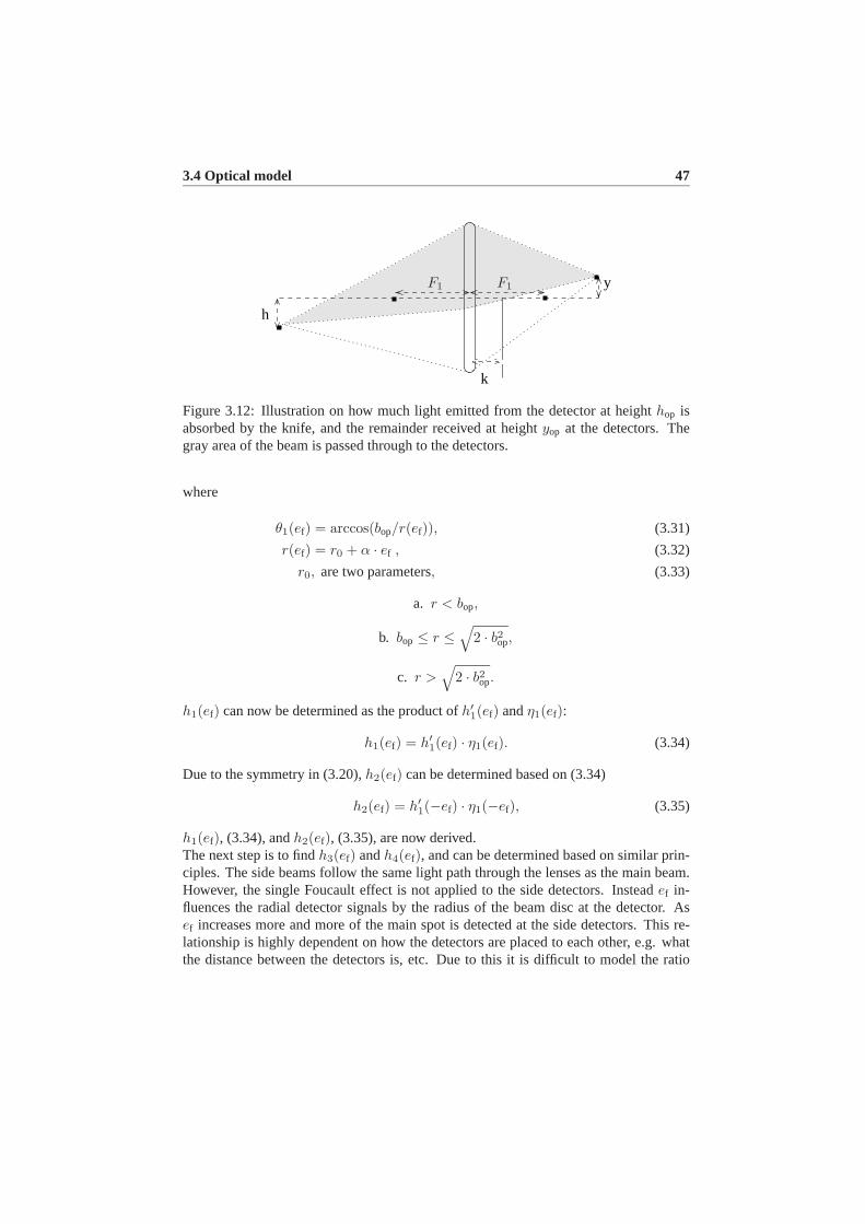
3.4 Optical model 47
y
k
h
F1F1
Figure 3.12: Illustration on how much light emitted from the detector at heighthop isabsorbed by the knife, and the remainder received at heightyop at the detectors. Thegray area of the beam is passed through to the detectors.
where
θ1(ef) = arccos(bop/r(ef)), (3.31)
r(ef) = r0 + α · ef , (3.32)
r0, are two parameters, (3.33)
a. r < bop,
b. bop ≤ r ≤√
2 · b2op,
c. r >√
2 · b2op.
h1(ef) can now be determined as the product ofh′1(ef) andη1(ef):
h1(ef) = h′1(ef) · η1(ef). (3.34)
Due to the symmetry in (3.20),h2(ef) can be determined based on (3.34)
h2(ef) = h′1(−ef) · η1(−ef), (3.35)
h1(ef), (3.34), andh2(ef), (3.35), are now derived.The next step is to findh3(ef) andh4(ef), and can be determined based on similar prin-ciples. The side beams follow the same light path through the lenses as the main beam.However, the single Foucault effect is not applied to the side detectors. Insteadef in-fluences the radial detector signals by the radius of the beam disc at the detector. Asef increases more and more of the main spot is detected at the side detectors. This re-lationship is highly dependent on how the detectors are placed to each other, e.g. whatthe distance between the detectors is, etc. Due to this it is difficult to model the ratio

48 Model of a Compact Disc Player
r
c)
b)a)
b
br
rb
Figure 3.13: Illustration on how the reflected light covers the detector and area outsidethe detector as radius of the reflected half disc beam increases. a)r < bop, b) bop ≤ r ≤√
2 · b2op and c)r >
√2 · b2
op
of the energy from the main spot is placed at the side detectors asef increases. Insteadthis part is approximated by a polynomial as a function ofef , meaningh
′3,4(ef) = p(ef).
Based on data this effect seems to dominate while the side spots are inside their de-tectors, they seems to grow out of there detectors at larger focus distance than for thetwo focus detectors. However, when the side spots start to grow out of their detectors theηi(ef)-function, see (3.30), this effect is clearly the main contribution to mapping. Thesetwo model cases are merged into one model, by using the polynomial for small valuesof ef and using the other part for larger values ofef . In Section 3.4.3 the parameters inthe models are identified based on measurements. The expression is as follows:
h3(ef) =
p(ef) if a)12 ·πr(ef)
2−r(ef)2·(2θ1(ef)−sin(2·θ1(ef)))12 ·πr(ef)2
· ks if b)2·b2
12 ·π·r(ef)2
· ks if c)
, (3.36)
where
θ1(ef) = arccos(bs/r(ef)), (3.37)
r(ef) = r0 + α · ef , (3.38)
p(ef) is a polynomial function ofef , (3.39)
ks = p(bs − r0
α), (3.40)
bs is the height of the detector. (3.41)
(3.42)
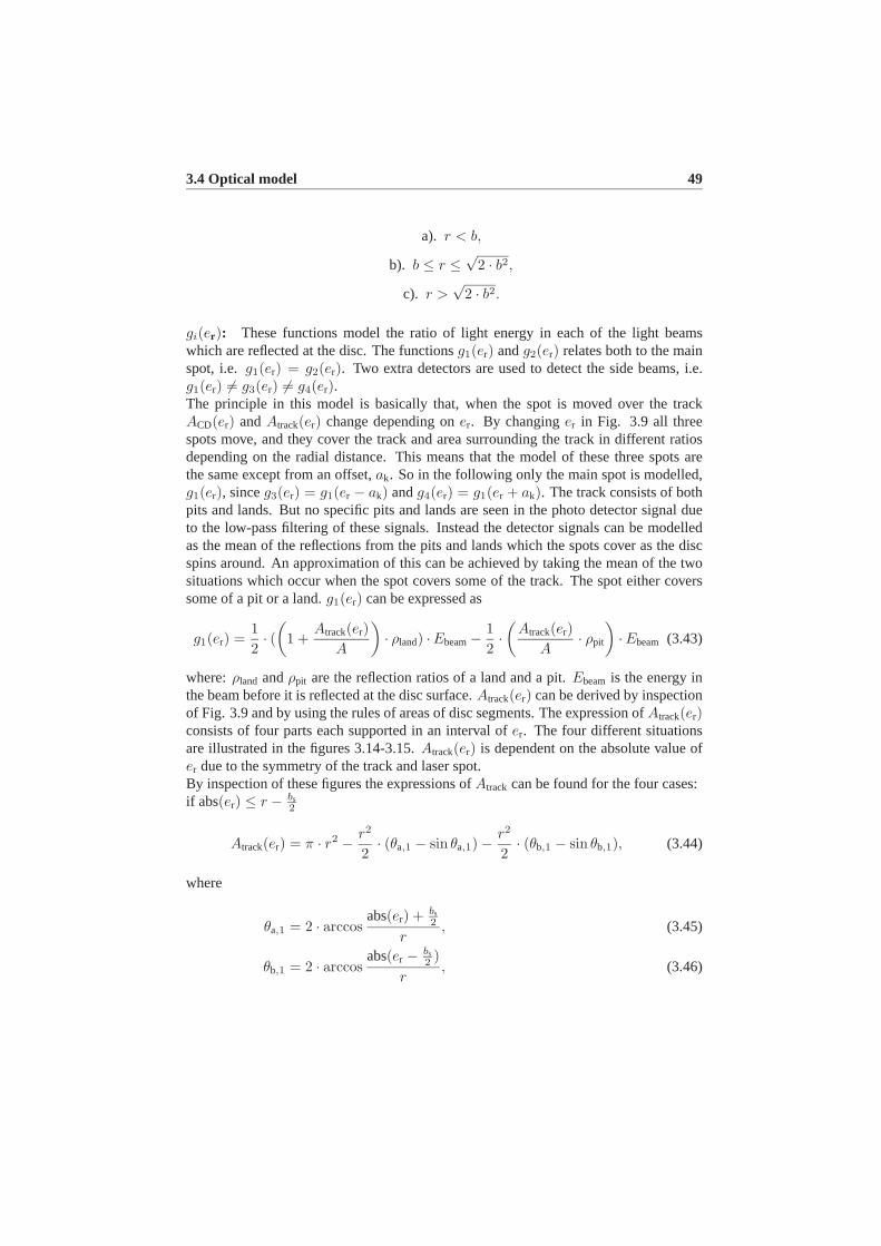
3.4 Optical model 49
a). r < b,
b). b ≤ r ≤√
2 · b2,
c). r >√
2 · b2.
gi(er ): These functions model the ratio of light energy in each of the light beamswhich are reflected at the disc. The functionsg1(er) andg2(er) relates both to the mainspot, i.e. g1(er) = g2(er). Two extra detectors are used to detect the side beams, i.e.g1(er) 6= g3(er) 6= g4(er).The principle in this model is basically that, when the spot is moved over the trackACD(er) andAtrack(er) change depending oner. By changinger in Fig. 3.9 all threespots move, and they cover the track and area surrounding the track in different ratiosdepending on the radial distance. This means that the model of these three spots arethe same except from an offset,ak. So in the following only the main spot is modelled,g1(er), sinceg3(er) = g1(er − ak) andg4(er) = g1(er + ak). The track consists of bothpits and lands. But no specific pits and lands are seen in the photo detector signal dueto the low-pass filtering of these signals. Instead the detector signals can be modelledas the mean of the reflections from the pits and lands which the spots cover as the discspins around. An approximation of this can be achieved by taking the mean of the twosituations which occur when the spot covers some of the track. The spot either coverssome of a pit or a land.g1(er) can be expressed as
g1(er) =12· (
(1 +
Atrack(er)A
)· ρland) ·Ebeam− 1
2·(
Atrack(er)A
· ρpit
)·Ebeam (3.43)
where:ρland andρpit are the reflection ratios of a land and a pit.Ebeamis the energy inthe beam before it is reflected at the disc surface.Atrack(er) can be derived by inspectionof Fig. 3.9 and by using the rules of areas of disc segments. The expression ofAtrack(er)consists of four parts each supported in an interval ofer. The four different situationsare illustrated in the figures 3.14-3.15.Atrack(er) is dependent on the absolute value ofer due to the symmetry of the track and laser spot.By inspection of these figures the expressions ofAtrack can be found for the four cases:if abs(er) ≤ r − bs
2
Atrack(er) = π · r2 − r2
2· (θa,1 − sin θa,1) − r2
2· (θb,1 − sin θb,1), (3.44)
where
θa,1 = 2 · arccosabs(er) + bs
2
r, (3.45)
θb,1 = 2 · arccosabs(er − bs
2 )r
, (3.46)
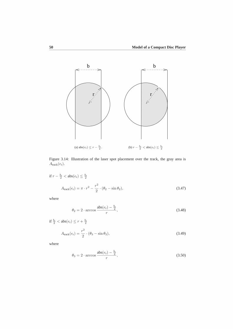
50 Model of a Compact Disc Player
b
r
(a) abs(er) ≤ r − bs2
.
b
r
(b) r − bs2
< abs(er) ≤ bs2
Figure 3.14: Illustration of the laser spot placement over the track, the gray area isAtrack(er).
if r − bs2 < abs(er) ≤ bs
2
Atrack(er) = π · r2 − r2
2· (θ2 − sin θ2), (3.47)
where
θ2 = 2 · arccosabs(er) − bs
2
r, (3.48)
if bs2 < abs(er) ≤ r + bs
2
Atrack(er) =r2
2· (θ3 − sin θ3), (3.49)
where
θ3 = 2 · arccosabs(er) − bs
2
r, (3.50)
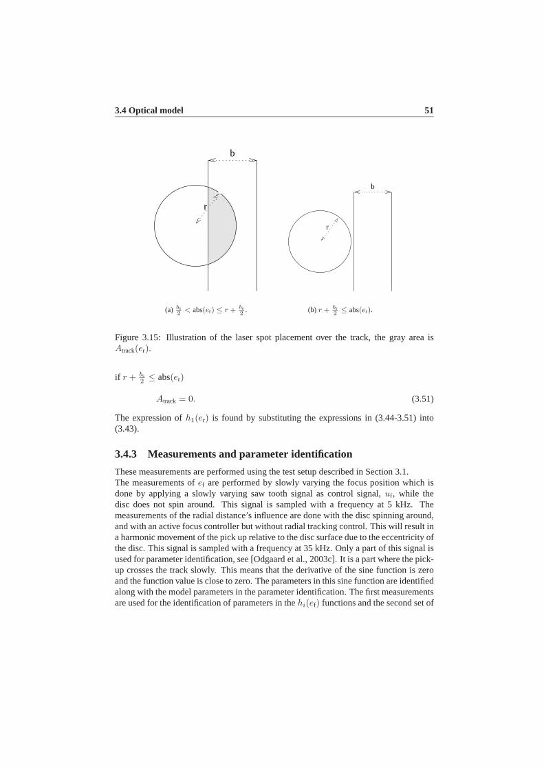
3.4 Optical model 51
b
r
(a) bs2
< abs(er) ≤ r + bs2
.
b
r
(b) r + bs2
≤ abs(er).
Figure 3.15: Illustration of the laser spot placement over the track, the gray area isAtrack(er).
if r + bs2 ≤ abs(er)
Atrack = 0. (3.51)
The expression ofh1(er) is found by substituting the expressions in (3.44-3.51) into(3.43).
3.4.3 Measurements and parameter identification
These measurements are performed using the test setup described in Section 3.1.The measurements ofef are performed by slowly varying the focus position which isdone by applying a slowly varying saw tooth signal as control signal,uf , while thedisc does not spin around. This signal is sampled with a frequency at 5 kHz. Themeasurements of the radial distance’s influence are done with the disc spinning around,and with an active focus controller but without radial tracking control. This will result ina harmonic movement of the pick up relative to the disc surface due to the eccentricity ofthe disc. This signal is sampled with a frequency at 35 kHz. Only a part of this signal isused for parameter identification, see [Odgaard et al., 2003c]. It is a part where the pick-up crosses the track slowly. This means that the derivative of the sine function is zeroand the function value is close to zero. The parameters in this sine function are identifiedalong with the model parameters in the parameter identification. The first measurementsare used for the identification of parameters in thehi(ef) functions and the second set of

52 Model of a Compact Disc Player
measurements are used forgi(er). Before doing the identification thehi(ef) andgi(er)are multiplied with a parameter due to the amplification in the detector and an offset isadded to this also due to the detectors.
The parameter identifications were done by using the MATLAB functionfminsearch to minimise the squared error of the difference between the mea-surements and model output, by changing the parameters. The initial parameters werefound partly in [Stan, 1998] and partly by trial and error. The model obtained withthe identified parameters is compared with the measurements in Figs. (3.16-3.19) asfunctions of eitherc · ef or er.
−10 −5 0 5 100
0.5
1
1.5
2
2.5
3
c*ef [v]
f 1 [v]
approximationmeasurements
(a)f1(c · ef , 0)
−10 −5 0 5 100
0.5
1
1.5
2
2.5
3
c*ef [v]
f 2 [v]
approximationmeasurements
(b) f2(c · ef , 0)
Figure 3.16: Measurements off1(c · ef , 0) andf2(c · ef , 0) compared with the simulatedf1(c · ef , 0) andf2(c · ef , 0). These two functions model the two focus detector signalsdependency of the focus distance.
The Figs. (3.16-3.19) show how the models in general have almost the same responseto the given inputs as the optical system. But due to some of the simplifications in themodel/assumptions, the models do not describe all phenomena in the optical detectorsystem. In Figs. 3.16(a), 3.16(b), 3.18(a) and 3.18(b) there are some bumps for largedisplacement, due to light from the other detector beams, which are not modelled. How-ever, these differences are not so important, concerning the purpose of this model, whichis in the control area. It can be corrected together with another model problem whichemerges in the further use of the optical model. This model is non differentiable at somepoints, even though the real optical system do not show such a behaviour. This is due topiecewise structure of the model. In [Odgaard et al., 2004a] and [Odgaard et al., 2003a],these problems are handled by approximating thehi(·) andgi(·) by cubic splines.
All the identified parameters can be seen in Appendix B.

3.5 Surface fault model 53
−4 −2 0 2 4 6
x 10−7
2.6
2.8
3
3.2
3.4
3.6
3.8
4
er [m]
f 1 [v]
approximationmeasurements
Figure 3.17: The focus detector as a function of the radial distance,f1(0, er), showingthe measured and simulated values.
3.5 Surface fault model
The purpose of the surface fault model and its related fault parameters are to use themfor fault detection and classification. In the following a realistic and simple model isfound. This model is as the optical model a static model, so the time variation of thevariables has been disregarded,
sm =
D1m
D2m
S1m
S2m
= fe(ef , er, αf , αr), (3.52)
sm is a vector of the measured photo detector signals. This model is related to the opticalmodel (3.17) by the following
fe(ef , er, 0, 0) = f(ef , er). (3.53)
It is seen by inspection that a fault decreasesD1 + D2 andS1 + S2. An example ofD1 + D2 sequence of a scratchy disc, Fig. 3.20. From this figure is it clear that a faultdecreasesD1 + D2.In [Odgaard et al., 2004a] a disturbance set is defined.
3.1 Definition (The disturbance set)The disturbance setD ∈ R4 is defined as the setin which any samplesm in R4 of the detector signals, will be if only disturbances occur.

54 Model of a Compact Disc Player
−10 −5 0 5 100
0.2
0.4
0.6
0.8
1
1.2
1.4
c*ef [v]
f 3 [v]
approximationmeasurements
(a)f3(c · ef , 0).
−10 −5 0 5 100
0.2
0.4
0.6
0.8
1
1.2
1.4
1.6
c*ef [v]
f 4 [v]
approximationmeasurements
(b) f4(c · ef , 0).
Figure 3.18: The radial detector as functions of the focus distance,f3(c · ef , 0) andf4(c · ef , 0). The figures compare the measured and simulated functionsf3(c · ef , 0) andf4(c · ef , 0).
−4 −2 0 2 4
x 10−7
0.7
0.8
0.9
1
1.1
1.2
1.3
1.4
1.5
er [m]
f 3 [v]
(a)f3(0, er).
−4 −2 0 2 4
x 10−7
0.5
1
1.5
er [m]
f 4 [v]
ApproximationMeasurements
(b) f4(0, er).
Figure 3.19: An illustration of the comparison of the measured and simulated radialdetectors dependence of the radial distances,f3(0, er) andf4(0, er).

3.5 Surface fault model 55
0 0.5 1 1.5 2 2.5 3
x 104
2.3
2.4
2.5
2.6
2.7
2.8
2.9
3
3.1
3.2
Samples [n]
D1+
D2 [V
]
Figure 3.20: AD1 + D2 sequence of a scratchy disc, notice the spikes which are thescratches.
To illustrate this disturbance set, a 2-dimensional version, where the two focus detectorsD1 andD2 are plotted in Fig. 3.21. The detector would be in the normal region ofD,if the focus distance is kept inside the normal operation region, the linear part of theoptical model. A fault can be viewed as a movement of the detector signals outside thisdisturbance set,D. In order to derive a model of the surface faults it is important todetermine the structure behind these movements outsideD.In [Odgaard et al., 2004a] two models are suggested. The first model is based on theassumption that the fault is orthogonal toD, at the point((ef , er), f(ef , er)). This orthog-onal model is illustrated in Fig. 3.22.The parameters in this fault model are two orthogonal distances:rf andrr, defined as:
rf =∥∥∥∥D1 − D1
D2 − D2
∥∥∥∥ , rr =∥∥∥∥S1 − S1
S2 − S2
∥∥∥∥ . (3.54)
These two parameters are also residuals, since they are equal to zero when no faultsoccur and increase as the fault increases.However, in cases of focus or radial distances unequal to 0 during the fault, the orthog-onal model will not be a good description of the fault, since experimental work in the2-dimensional case, in [Vidal et al., 2001a], indicates what all detector signals tend to-wards the origin during a fault. This could indicate that it would be better to model thefault with a scale,β, multiplied with s, as the first parameter andγ which is the modelerror as the second parameter:
sm ≈ β · s, γ = ||sm − β · s||, (3.55)

56 Model of a Compact Disc Player
Normal region
D1
D2
Figure 3.21: A 2-dimensional illustration of the disturbance set.D2 as a function ofD1
for small focus distances, inside the normal operation region. The dashed line illustratesdetector signal path outside the normal region.
Normal region
Defect
direc
tion
D1
D2
Figure 3.22: A 2-dimensional illustration of an orthogonal fault model. The fault movesthe detector signals outside the normal operation region. The dashed line illustratesdetector signal path outside the normal region.

3.5 Surface fault model 57
Normal region
Defect d
irecti
on
D1
D2
Figure 3.23: A 2-dimensional illustration of a scaling fault model. The fault moves thedetector signals outside the normal operation region. The dashed line illustrates detectorsignal path outside the normal region.
β is not a residual since it is 1 if no fault occurs and decreases as the fault develops.Instead a residual,α, can be found based onβ by:
α = 1 − β. (3.56)
This scaling model is illustrated in Fig. 3.23. Since only one fault variable is used, thisfault model does not guarantee thatsm can be reconstructed based onef , er, β. As aconsequence other model structures were tested. These experiments showed that a wellsuited model structure is to use one scaling for the focus detectors and another scalingfor the radial detectors.
sm =[βf · I 00 βr · I
]· s, (3.57)
and the residuals based onβf andβr can be constructed as[αf
αr
]=
[1 − βf
1 − βf
]. (3.58)
These two residuals can be used for fault detection, with a clear improving potential, seeSection 4.4, [Odgaard et al., 2003b] and [Odgaard et al., 2003a].These fault parameters parameterise the main part of the surface faults. Unfortunatelythe surface faults also contribute with energy in the focus and radial distances, or in

58 Model of a Compact Disc Player
other words surface faults introduce additional faulty focus and radial distance signalcomponents. If these faulty focus and radial distance components are denoted:ef ander, a fault model can be defined as
sm =[βf · I 00 βr · I
]· f (ef + ef , er + er) . (3.59)
Notice thatβf andβr are very useful for fault detection etc, but it isef ander which causethe problem for the controllers during a surface fault.
3.6 Summary
This chapter was devoted to the modelling of the focus and radial servos in a CD-player,with a main focus on the optical model and a model of surface faults. The model isdeveloped to model the used experimental test setup. This experimental test setup isdescribed in Section 3.1. The general model structure was described in Section 3.2. InSection 3.3 a simple dynamical model of the electro-magnetic-mechanical system wassummarised. An often missed part of the focus and radial servos, the optical system wasmodelled with cross-couplings in Section 3.4. In Section 3.5 a model structure of thesurface faults was presented.
Chapter 4
Fault Residuals Based onEstimations of the Optical Model
In this chapter the inverse map of the combined optical and surface fault model is solved.To understand the importance of this inverse map, one should notice the following re-marks on the modelling done in the previous chapter. In Chapter 3 the focus and radialservos were modelled. The dynamic model of the electro-magnetic-mechanical systemwas first derived. Normally the detector signals are used directly to compute the feed-back signals and the residuals. These computations are based on simple linear modelsof the optical system in the OPU, and without any models of the surface faults. Thehandling of these surface faults is the main topic in this work. A static non-linear modelof the optical system was derived in Chapter 3 together with a static model of the surfacefaults. These two models are defined by mappings from the focus and radial distancesand the two fault parameters to the four detector signals. The inverse map of this map-ping gives focus and radial distances together with some fault parameters. The faultparameters defined in Section 3.5 are decoupled from the cross-coupling from the otherservo loop. The sum signals depend on the respective other focus or radial distancesdue to the optical cross-couplings. As a consequence it is problematic to use these sumsignals as residuals, but they are used due to the lack of better alternatives. This problemwith the optical cross-couplings can be avoided by solving the inverse map and insteaduse the fault parameters and their derived residuals. Unfortunately, the non-linear opticalmodel does not have a globally defined solution. Instead an iterative method to computethe inverse map is used, based on Newton-Raphson’s method and a Kalman estimator.In Section 4.1, the structure of this inverse problem solver is described. This is followedby the solution of the inverse map based on an iterative method, see Section 4.2. AKalman estimator is introduced and designed in Section 4.3, in order to estimate the realfocus and radial distances during surface faults. In Section 4.3 the method is used onsome experimental data. In Section 4.4 the potentials of the new decoupled residuals are
59

60 Fault Residuals Based on Estimations of the Optical Model
illustrated by a fault detection example.
4.1 The structure of the inverse map solver
In the normal servo system indirect measures of focus and radial distances are used.These indirect measures of the distances are found by taking the normalised differencebetween the two focus and the two radial detector signals. It is important to distinguishbetween disturbances, which the controller shall reject and faults which the controllershall not react to. If preconditioning of the measurements are not used it might make theseparation of disturbances from faults more difficult. There are two problems with themeasures. The first problem is that there are cross-couplings between the focus distanceand the radial detector signals and between the radial distance and focus detector signals.The second problem is that the mappings from the distances to the indirect measures arelinear only for small distances. Both these problems lead to the fact that it would bebetter to establish estimates of focus and radial distances for the controlling of the focusand radial distances, by solving the inverse map of the optical model. It is at least asimportant that this inverse map can be used to compute some residuals with a clearseparation property compared with the normally used ones.By solving the inverse map of the combined optical and fault model, (3.59), one gets:βf [n], βr[n], ef [n] + ef [n] ander[n] + er[n]. A Kalman estimator can following be usedto estimate the physical focus and radial distances:ef [n] ander[n], which result in thedynamical estimates of focus and radial distances:ef [n] and er[n]. In other words theKalman estimator opens the closed loop, the two remainders are the open loop faults anddisturbances. The two remainders contain more than the faulty distance components dueto the surface faults,ef [n] ander[n], the remainder also contain measurement noises anddisturbances as well. The measurement noises and disturbances can be assumed to bestochastic. The surface faults do not vary much from encounter to encounter, see Fig.4.1 and [Odgaard et al., 2004d].The used Kalman estimator is a Kalman estimator with an internal reference model. Theinternal reference model is a model of the eccentricity and skewness of the disc. TheKalman estimatesef [n] ander[n] can e.g. be used as partial state estimates to a controller,or fed into the optical model, with the purpose of estimating the detector signals,s[n],the difference from these estimates to the measured distances are open loop estimates offaults and disturbances influencing the system. This dynamical estimate of the detectorsignals can together withef [n] and er[n] be used for extraction of the fault parametersand residuals.A method is suggested for extraction and estimation of focus and radial distances andfault parameters/residuals. These signals can be used to improve the performance of thenominal and the feature based controllers for a CD-player. The system is illustrated inFig. 4.3. The inverse map solver finds static estimates of optical distances from sampleddetector signals.

4.1 The structure of the inverse map solver 61
0 20 40 60 80 100 120 140 1600
20
40
60
80
2.7
2.8
2.9
3
3.1
3.2
3.3
3.4
3.5
x
z
y
Figure 4.1: 3-D plot ofβf [n] in sequential fault encounters. The duration and depth ofthe fault increases. The x-axis is samples ofyth encounter, (the y-axis is the encounternumber), and the z-axis isβf [n].
Surface FaultsystemOptical
Electro−
magneticsystem
u
d
dref
s smef , er
Figure 4.2: The principles of the model of the CD-player. The CD-player consists offour parts. The electro-magnetic-mechanical system and the optical system, the vectorof unknown referencesdref(t) and the surface fault.u(t) is a vector of the control signalto the electro-magnetic system,d(t) is a vector of the unknown disturbances to theelectro-magnetic-mechanical system,dref(t) is a vector of the unknown reference to thesystem,ef(t) is a vector of the focus distance,er(t) is a vector of the radial distance,sm(t) is a vector of the measured detector signals, ands(t) is a vector of detector signalswithout surface faults.

62 Fault Residuals Based on Estimations of the Optical Model
InverseMap Estimator
Kalman CD player
u sm ef , er
ef , erαf , αr
Figure 4.3: The structure of the method described in this chapter. The method consistsof two parts, which estimate fault parameters, (αf , αr), focus distance and radial distancefrom the detector signals. The parts of the method are: inverse map solver and Kalmanestimator.u is a vector of the control signals to the CD-player, see Fig. 4.2,sm is avector of the measured detector signals,ef , er is the static estimated focus and radialdistances, andef , er is the dynamical estimated focus and radial distances.
S1
S2
ssm
f
Figure 4.4: Due to a fault the measured detector signal,sm[n], lies outside the output setof the optical model,f(·). This is illustrated with the detector signalsS1 andS2, whereef = 0 implying thatf(·) is a curve in theS1-S2 plane and constant inD1 andD2.
The method consists of two parts each depending on each other. The first part is theinverse map of the optical and the fault model.The four detector signals can be described as in (3.59).fe(·) is an extended modelcombining the optical model and a fault model.f(·) is the optical model, which mapsinto a 2-dimensional manifold embedded in a 4-dimensional space.Combining the model and the four detector signals gives four equations with 2 variablesconcerning the computation of the two distances. In order to describe the 4-dimensionalspace two extra variables are used to describe the deviation. These variables are theimplicit fault model, parameterised byαf [n] andαr[n]. This means that the solution tothis problem is to compute the inverse map offe(·). The inverse is not globally defined,meaning that the solver only finds a local solution.In Definition 3.1 in Section 3.5 the disturbance setD ∈ R4 was defined.
4.2 Solutions of the inverse map 63
The extended model output for two detector signals is illustrated in Fig. 4.4. This figureillustrates a sampling ofS1 andS2, outsideD due to a fault.
4.2 Solutions of the inverse map
The solution of the inverse map can be found based on the use of the fault model and theoptical model. The method and algorithm are described in [Odgaard et al., 2004a] and[Odgaard et al., 2003a]. The method is based on the following facts. Due to low passfiltering nature of the OPU the following limits are relevant:|ef [n]− ef [n+1]| < µf and|er[n]−er[n+1]| < µr, wheren is any sample, andµf andµr are the maximum changesin ef [n] ander[n], see [Odgaard et al., 2004a] and [Odgaard et al., 2003a]. Based on thestandard requirements to the CD-player servos, see [Stan, 1998], the maximum deviationof focus and radial positions from sample to sample can be calculated to:µf = µr ≈0.014µm.In the following an approach is described, which locally computes the inverse map andthereby find the right candidate point, and use this to compute the fault parameters andrelated residuals.
4.2.1 The scaling projection method
The problem is to find the point,f(e[n]) in D, wheree[n] =[ef [n] er[n]
]T. If the
model output is substituted into (3.57) the following is achieved
sm[n] = B[n] · f(e[n]), (4.1)
where
B[n] =[βf [n] · I 0
0 βr[n] · I]
. (4.2)
For computational reasons, a new matrixB∗[n] is defined,
B∗[n] =[β−1
f [n] · I 00 β−1
r [n] · I]
. (4.3)
Unfortunately, due to the shape ofD in R4, there are a number of points inD forwhich (4.1) will be true. However, due to the system’s low-pass-filtering effecte[n] isexpected to be neare[n−1], this means that if an iterative algorithm is used to finde[n],e[n−1] can be used as a starting value of the algorithm. Experiments have shown that itimproves results if the dynamically estimated distances are used as this start value. I.e:
e0[n] =[ef [n] er[n]
]T. Using these low-pass-filtered-estimated distances as initial
values for the algorithm, noises etc. are removed from the initial value. This results in
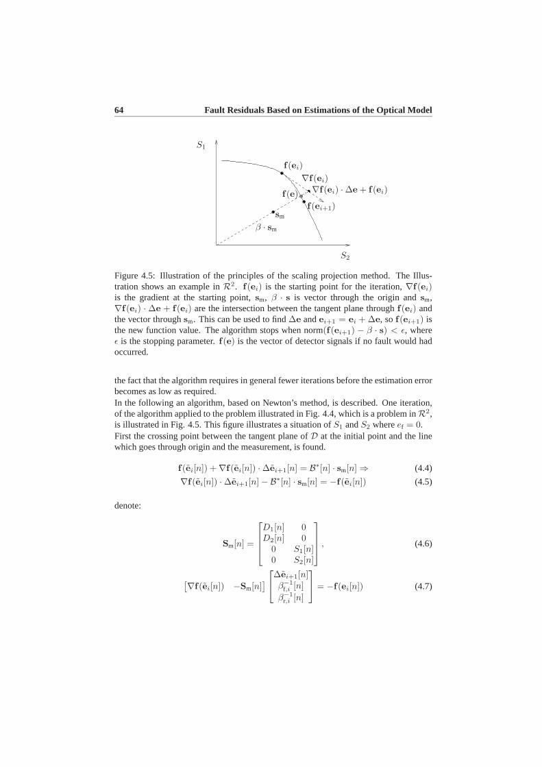
64 Fault Residuals Based on Estimations of the Optical Model
f(ei)∇f(ei)
sm
β · sm
f(ei+1)f(e) ∇f(ei) · ∆e + f(ei)
S1
S2
Figure 4.5: Illustration of the principles of the scaling projection method. The Illus-tration shows an example inR2. f(ei) is the starting point for the iteration,∇f(ei)is the gradient at the starting point,sm, β · s is vector through the origin andsm,∇f(ei) · ∆e + f(ei) are the intersection between the tangent plane throughf(ei) andthe vector throughsm. This can be used to find∆e andei+1 = ei + ∆e, sof(ei+1) isthe new function value. The algorithm stops when norm(f(ei+1) − β · s) < ε, whereε is the stopping parameter.f(e) is the vector of detector signals if no fault would hadoccurred.
the fact that the algorithm requires in general fewer iterations before the estimation errorbecomes as low as required.In the following an algorithm, based on Newton’s method, is described. One iteration,of the algorithm applied to the problem illustrated in Fig. 4.4, which is a problem inR2,is illustrated in Fig. 4.5. This figure illustrates a situation ofS1 andS2 whereef = 0.First the crossing point between the tangent plane ofD at the initial point and the linewhich goes through origin and the measurement, is found.
f(ei[n]) + ∇f(ei[n]) · ∆ei+1[n] = B∗[n] · sm[n] ⇒ (4.4)
∇f(ei[n]) · ∆ei+1[n] − B∗[n] · sm[n] = −f(ei[n]) (4.5)
denote:
Sm[n] =
D1[n] 0D2[n] 0
0 S1[n]0 S2[n]
, (4.6)
[∇f(ei[n]) −Sm[n]] ∆ei+1[n]
β−1f,i [n]
β−1r,i [n]
= −f(ei[n]) (4.7)

4.2 Solutions of the inverse map 65
The left most matrix in (4.7) is in practice invertible, since it has full rank, except from afew situations of low dimension. These situations can be avoided if the initial point forthe iterations is in the nominal range of operations.
∆ei+1[n]
β−1f,i [n]
β−1r,i [n]
= − ([∇f(ei[n]) −Sm[n]
])−1 · f(ei[n]). (4.8)
Using all four parameters to model the received detector signals, the detector signalswill be fully parameterised and is possible to achieve a zero model error. The algorithmwill converge to the solution if it is in the vicinity of the solution, which it is due to thelimited change in focus and radial distances from sample to sample. This means that thesuggested algorithm will converge as follows:limi→∞ ei[n] = e[n], limi→∞ ef,i[n] =ef [n], limi→∞ er,i[n] = er[n].It is thereby relevant to use theL2 norm of the difference between estimated and mea-sured detector signals, as the stop criteria for the algorithm:∥∥(f(e[n]) − β[n] · sm[n])
∥∥2
< ε. (4.9)
If the stop criteria is fulfilled, the algorithm stops, and if not fulfilled, the computeddistances are used as initial guess for the next iteration. When the algorithm is stoppedthe residuals are computed.
From fault parameters to residuals In fault detection residuals are used to detectfaults (surface faults). In this terminology a residual means more than just a differencebetween two signals, e.g. the difference between measured and estimated system out-puts. In [Chen and Patton, 1991] a residual is defined to be zero for the fault-free caseand nonzero for the fault free case. In this case the fault parametersβf [n] andβr[n] areequal to 1 in the fault free case and decreases towards 0 in case of a fault. The faultparameters can be converted to residualsαf [n] andαr[n][
αf [n]αr[n]
]=
[1 − βf [n]1 − βr[n]
]. (4.10)
4.2.1.1 The algorithm
1. Find the gradient,∇f(ei[n]) to the point(ei[n], f(ei[n])).
2. Compute:ei+1[n]
βf,i[n]βr,i[n]
=
ei[n]
00
− ([∇f(ei[n]) −Sm[n]
])−1 · f(ei[n]).
3. Compute:γ[n] =∥∥Bi[n]sm[n] − f(ei+1[n])
∥∥2
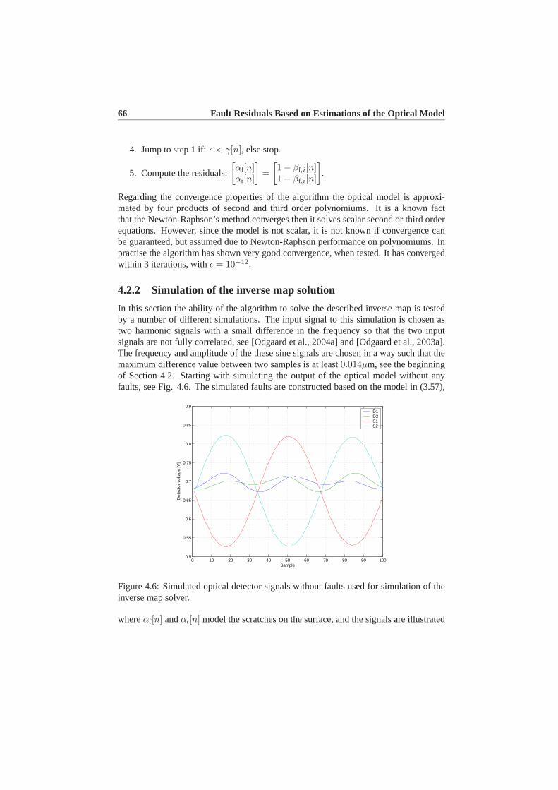
66 Fault Residuals Based on Estimations of the Optical Model
4. Jump to step 1 if:ε < γ[n], else stop.
5. Compute the residuals:
[αf [n]αr[n]
]=
[1 − βf,i[n]1 − βf,i[n]
].
Regarding the convergence properties of the algorithm the optical model is approxi-mated by four products of second and third order polynomiums. It is a known factthat the Newton-Raphson’s method converges then it solves scalar second or third orderequations. However, since the model is not scalar, it is not known if convergence canbe guaranteed, but assumed due to Newton-Raphson performance on polynomiums. Inpractise the algorithm has shown very good convergence, when tested. It has convergedwithin 3 iterations, withε = 10−12.
4.2.2 Simulation of the inverse map solution
In this section the ability of the algorithm to solve the described inverse map is testedby a number of different simulations. The input signal to this simulation is chosen astwo harmonic signals with a small difference in the frequency so that the two inputsignals are not fully correlated, see [Odgaard et al., 2004a] and [Odgaard et al., 2003a].The frequency and amplitude of the these sine signals are chosen in a way such that themaximum difference value between two samples is at least0.014µm, see the beginningof Section 4.2. Starting with simulating the output of the optical model without anyfaults, see Fig. 4.6. The simulated faults are constructed based on the model in (3.57),
0 10 20 30 40 50 60 70 80 90 1000.5
0.55
0.6
0.65
0.7
0.75
0.8
0.85
0.9
Sample
Det
ecto
r vo
ltage
[V]
D1D2S1S2
Figure 4.6: Simulated optical detector signals without faults used for simulation of theinverse map solver.
whereαf [n] andαr[n] model the scratches on the surface, and the signals are illustrated

4.3 Kalman estimator 67
0 10 20 30 40 50 60 70 80 90 1000.84
0.86
0.88
0.9
0.92
0.94
0.96
0.98
1
1.02
Sample
Gai
n
Figure 4.7: The focus and radial residualsαf [n] andαr[n] time series, which are used asthe surface faults in this simulation.
in Fig. 4.7, in this simulationαf [n] = αr[n]. Using the fault model and the fault signal inFig. 4.7, the simulation series of samples with surface faults are computed and illustratedin Fig. 4.8. Before using the algorithm on these test data, independent random noisesare added to the four detector signals, to simulate disturbances and measurement noises.The next step in the simulation is to apply the signal from Fig. 4.8 to the algorithm.In this simulation the detector signals shown in Fig. 4.8 are fed to the algorithm. Theresults are shown in Fig. 4.9. In Fig. 4.9f(e[n]) is illustrated. From this plots it is clearthat the scaling projection method is well suited for solving this inverse map with thegiven fault model.
4.3 Kalman estimator
In Fig. 4.9 the measurement noises, faulty focus and radial distances components areremaining after the solution of the inverse map. The computed focus and radial distancesare when mapped through the optical model before its appearance in Fig. 4.9. In order toremove these measurement noises and faulty focus and radial distance components fromthe computed focus and radial distances, a Kalman estimator is designed to estimate thefocus and radial distances as a response of the control signals. In addition this Kalmanestimator can be used to give an estimate of the faults and disturbances with the systemresponse to these.The reference signals to focus and radial loops are unknown. The nature of these ref-

68 Fault Residuals Based on Estimations of the Optical Model
0 10 20 30 40 50 60 70 80 90 1000.45
0.5
0.55
0.6
0.65
0.7
0.75
0.8
0.85
0.9
Sample
Det
ecto
r vo
ltage
[V]
D1D2S1S2
Figure 4.8: Simulation of the four detector signals,D1[n], D2[n], S1[n] andS2[n], withsurface faults and measurement noises.
erences is eccentricity and skewness of disc etc. However, it is known that the first andmost dominant harmonic of the unknown reference is the angular velocity of the disc.The interval of the angular velocity can be retrieved from [Stan, 1998] to be4 − 9Hz.One way to model the reference is by a bandpass filter with the bandpass region between4 and 9 Hz. The model will be of the structure:
ηref(t) = Aref · ηref(t) + Eref · qref(t), (4.11)
dref(t) = Cref · ηref(t), (4.12)
where:ηref(t) is the state vector of the internal reference model,dref(t) is the reference,qref(t) is the input to internal reference model which is a white noise signal.
The focus and radial electro-magnetic-mechanical models given in (3.11 -3.12) are trans-form to a states-pace representation. It is following possible to merge the internal refer-ence model with focus and radial models.
ηCD(t) = ACD · ηCD(t) + BCD · uCD(t) + E · qref(t), (4.13)[ef(t)er(t)
]= CCD · ηCD(t), (4.14)

4.3 Kalman estimator 69
0 10 20 30 40 50 60 70 80 90 1000.5
0.55
0.6
0.65
0.7
0.75
0.8
0.85
0.9
Sample
Det
ecto
r vo
ltage
[V]
Est. D1
Est. D2
Est. S1
Est. S2
Figure 4.9: Illustration of the estimation of the four detector signals,D1[n], D2[n], S1[n]andS2[n] by the use of the scaling projection method.
where
ACD =
Af 0 0 00 Ar,f 0 0,0 0 Ar 00 0 0 Ar,r
∈ R8×8, (4.15)
BCD =
Bf 00 00 Br,0 0
∈ R8×2, (4.16)
CCD =[Cf Cr,f 0 00 0 Cr Cr,r
]∈ R2×8, (4.17)
E =
0 0Er,f 00 000 Er,r
∈ R8×2, (4.18)
whereAf ,Bf ,Cf are the model matrices in the focus model, andAr,Br,Cr are themodel matrices in the radial model.Ar,f,Cr,f,Er,f are the matrices of the focus referencemodel, andAr,r,Cr,r,Er,r are the matrices of the radial reference model.Before designing the Kalman estimator, the dynamical model of the electro-magnetic-mechanical system is discretised and expanded to include state and measurement noises
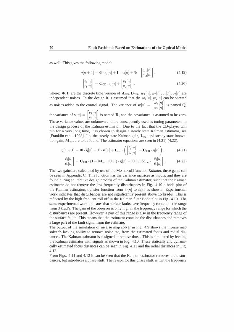
70 Fault Residuals Based on Estimations of the Optical Model
as well. This gives the following model:
η[n + 1] = Φ · η[n] + Γ · u[n] + Ψ ·[w1[n]w2[n]
], (4.19)[
ef [n]er[n]
]= CCD · η[n] +
[v1[n]v2[n]
], (4.20)
where:Φ,Γ are the discrete time version ofACD,BCD. w1[n], w2[n], v1[n], v2[n] areindependent noises. In the design it is assumed that thew1[n], w2[n] can be viewed
as noises added to the control signal. The variance ofw[n] =[w1[n]w2[n]
]is namedQ,
the variance ofv[n] =[v1[n]v2[n]
]is namedR, and the covariance is assumed to be zero.
These variance values are unknown and are consequently used as tuning parameters inthe design process of the Kalman estimator. Due to the fact that the CD-player willrun for a very long time, it is chosen to design a steady state Kalman estimator, see[Franklin et al., 1998]. I.e. the steady state Kalman gain,L∞, and steady state innova-tion gain,M∞, are to be found. The estimator equations are seen in (4.21)-(4.22):
η[n + 1] = Φ · η[n] + Γ · u[n] + L∞ ·([
ef [n]er[n]
]− CCD · η[n]
), (4.21)[
ef [n]er[n]
]= CCD · (I − M∞ · CCD) · η[n] + CCD · M∞ ·
[ef [n]er[n]
]. (4.22)
The two gains are calculated by use of the MATLAB functionKalman, these gains canbe seen in Appendix C. This function has the variance matrices as inputs, and they arefound during an iterative design process of the Kalman estimator, such that the Kalmanestimator do not remove the low frequently disturbances In Fig. 4.10 a bode plot ofthe Kalman estimators transfer function fromef [n] to ef [n] is shown. Experimentalwork indicates that disturbances are not significantly present above 15 krad/s. This isreflected by the high frequent roll off in the Kalman filter Bode plot in Fig. 4.10. Thesame experimental work indicates that surface faults have frequency content in the rangefrom 3 krad/s. The gain of the observer is only high in the frequency range for which thedisturbances are present. However, a part of this range is also in the frequency range ofthe surface faults. This means that the estimator contains the disturbances and removesa large part of the fault signal from the estimate.The output of the simulation of inverse map solver in Fig. 4.9 shows the inverse mapsolver’s lacking ability to remove noise etc, from the estimated focus and radial dis-tances. The Kalman estimator is designed to remove those. This is simulated by feedingthe Kalman estimator with signals as shown in Fig. 4.10. These statically and dynami-cally estimated focus distances can be seen in Fig. 4.11 and the radial distances in Fig.4.12.From Figs. 4.11 and 4.12 it can be seen that the Kalman estimator removes the distur-bances, but introduces a phase shift. The reason for this phase shift, is that the frequency

4.3 Kalman estimator 71
Frequency (rad/sec)
Pha
se (
deg)
; Mag
nitu
de (
dB)
Bode Diagrams
−30
−20
−10
0
10
100
101
102
103
104
105
106
−80
−60
−40
−20
0
20
Figure 4.10: Bode plot of the Kalman estimator’s transfer function fromef [n] to ef [n].
0 10 20 30 40 50 60 70 80 90 100−1
−0.8
−0.6
−0.4
−0.2
0
0.2
0.4
0.6
0.8
1x 10
−6
Samples [n]
Foc
us d
ista
nce
[m]
efef
Figure 4.11: The statically and dynamically estimated focus distance signals used in thesimulation of the inverse mapping solver.
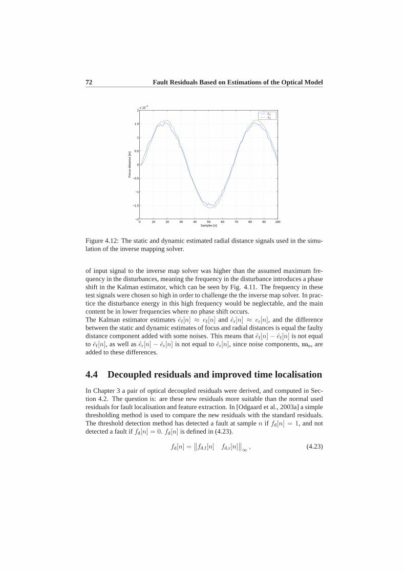
72 Fault Residuals Based on Estimations of the Optical Model
0 10 20 30 40 50 60 70 80 90 100−2
−1.5
−1
−0.5
0
0.5
1
1.5
2x 10
−8
Samples [n]
Foc
us d
ista
nce
[m]
erer
Figure 4.12: The static and dynamic estimated radial distance signals used in the simu-lation of the inverse mapping solver.
of input signal to the inverse map solver was higher than the assumed maximum fre-quency in the disturbances, meaning the frequency in the disturbance introduces a phaseshift in the Kalman estimator, which can be seen by Fig. 4.11. The frequency in thesetest signals were chosen so high in order to challenge the the inverse map solver. In prac-tice the disturbance energy in this high frequency would be neglectable, and the maincontent be in lower frequencies where no phase shift occurs.The Kalman estimator estimatesef [n] ≈ ef [n] and er[n] ≈ er[n], and the differencebetween the static and dynamic estimates of focus and radial distances is equal the faultydistance component added with some noises. This means thatef [n] − ef [n] is not equalto ef [n], as well aser[n] − er[n] is not equal toer[n], since noise components,mn, areadded to these differences.
4.4 Decoupled residuals and improved time localisation
In Chapter 3 a pair of optical decoupled residuals were derived, and computed in Sec-tion 4.2. The question is: are these new residuals more suitable than the normal usedresiduals for fault localisation and feature extraction. In [Odgaard et al., 2003a] a simplethresholding method is used to compare the new residuals with the standard residuals.The threshold detection method has detected a fault at samplen if fd[n] = 1, and notdetected a fault iffd[n] = 0. fd[n] is defined in (4.23).
fd[n] =∥∥fd,f [n] fd,r[n]
∥∥∞ , (4.23)

4.4 Decoupled residuals and improved time localisation 73
0 100 200 300 400 500 600 700 8000.35
0.4
0.45
0.5
0.55
0.6
0.65
0.7
0.75
samples
scal
ed d
etec
tor
sign
als
D1D2S1S2
Figure 4.13: Measured detector signalsD1[n],D2[n], S1[n] andS2[n] while passing thescratch.
where
fd,i[n] =
{1 if ri[n] > λi,
0 if ri[n] < λi,(4.24)
i ∈ {f, r}, (4.25)
where r[n] is the residual tested, in the tests two sets of residuals are tested,{αf [n], αr[n]} and {Sf [n], Sr[n]}. λi is the thresholds.{Sf [n], Sr[n]} are the nor-mally used residuals for surface fault detection - they are defined as followsSf [n] =D1[n] + D2[n] andSr[n] = S1[n] + S2[n]. This pair of residuals are also a represen-tation of the light reflection rate, but without taking cross couplings and non-linearitiesinto account. The new residuals are compared to these coupled residuals by the used ofa normal thresholding algorithm. The original scratch can be seen in Fig. 4.13. Theseresults can be seen in Figs. 4.14 and 4.15. Fig. 4.14 illustrates the localisation basedon the normal and new focus residual, and Fig. 4.15 illustrates the localisation basedon the normal and new radial residual. The original scratch can be seen in Fig. 4.15.The thresholds for the given signals are found such that they detect as much of the faultas possible and without making any false detections on the test data. These thresholdsare found by a trial and error method. Starting with Fig. 4.13 which illustrates thescaled detector signals, since it is easy from this figure to do a visual detection of thescratch. The real scratch is the part of the signals where the values are decreased. Itlasts approximately from sample 230 to sample 670. The ideal fault detection algorithmwill end up with these beginning and end detections of the scratch which, however, is a

74 Fault Residuals Based on Estimations of the Optical Model
225 230 235 240 245−0.02
0
0.02
0.04
0.06
0.08
0.1
samples [n]
scal
e [ ]
660 662 664 666 668 670 672 674 676 678 680−0.02
0
0.02
0.04
0.06
0.08
0.1
samples [n]
scal
e [ ]
αf
Detect 1Detect 2
αf
Detect 1Detect 2
Figure 4.14:αf [n] plotted together with detection signals based on bothαf [n] (Detect 1)andSf [n] (Detect 2). The upper plot shows the beginning detection of the scratch, andthe lower plot shows the end detection
225 230 235 240 245−0.02
0
0.02
0.04
0.06
0.08
0.1
samples [n]
scal
e [ ]
660 662 664 666 668 670 672 674 676 678 680−0.02
0
0.02
0.04
0.06
0.08
0.1
samples [n]
scal
e [ ]
αr
Detect 1Detect 2
αr
Detect 1Detect 2
Figure 4.15:αr[n] plotted together with detection signals based on bothαr[n] (Detect 1)andSr[n] (Detect 2). The upper plot shows the beginning detection of the scratch, andthe lower plot shows the end detection.

4.5 Summary 75
hard requirement to fulfill. Figs. 4.14 and 4.15 illustrates the beginning and end of thescratch seen in Fig. 4.13.From Figs. 4.14 and 4.15 it can be seen thatSf [n], Sr[n], αr[n] andαr[n] are goodfault parameters/ residuals for detection of the fault, since the size of the variations inthe residuals during the scratch are significantly larger than the variations due to noisesoutside the scratch. Based on these residuals a threshold detection is implemented, byusing a threshold which gives the earliest detection of the scratch without giving falsedetections, (the thresholds were found by lowering these thresholds until false detectionswere present). The detections based on the four residuals are: theαs : n = [233−668],the Ss : n = [239 − 665]. From these it can be seen that fault detection based onthe new decoupled residualsαf [n] and αf [n] give a more clear detection than if thetwo other residuals were used, since the background noise level is lower. The newresiduals have an improvement of 6 samples in the beginning and 3 samples in the end.This improvement seems less significant compared to duration of the scratch which is441 samples, but many practical experiments with fault tolerant control in CD-playershave shown that an improvement of a few samples of the fault detection means a lotin the achieved controller performances. One should also note that the new method fordetection is very close to the fault localisation by the visual inspection. If these twomethods are compared one can see that the extended threshold method has an error of3 samples in the beginning and only 2 sample in the end, on the other hand the faultdetection based on the normal residuals had an error of 9 samples in the beginning and5 in the end.In additionαf [n] andαr[n] are by construction decoupled from the respective radial andfocus distances, see [Odgaard et al., 2004a]. As it has been shown earlier the sum signalshave a non-linear coupling. In this example the thresholds used for the sum signals werenot chosen in the way that the detection is robust towards the optical cross-couplings,meaning that if the detection should be robust towards the cross-couplings the thresholdwould need to be increased. In turn this would imply that the beginning of the faultwould be detected later and the end earlier.This example makes it clear that it worthwhile to use these new residuals in the timelocalisaton and feature extraction of the faults in the following chapters, this time local-isation and feature extraction will be the topic, starting with some required theory in thefield of time/frequency analysis.
4.5 Summary
In this chapter, a method to solve the inverse map of the combined non-linear optical andfault models, was described. By solving this inverse map, two fault parametersβf [n] andβr[n] can be computed as well as an estimate of focus and radial distancesef [n] ander[n].These four parameters parameterise the four dimensional detector space.βf [n] andβr[n]are transformed into two related residualsαf [n] andαr[n].In Section 4.1 the overall solver structure is presented, where a Newton-Raphson based

76 Fault Residuals Based on Estimations of the Optical Model
iterative method is used to solve the inverse map, see Section 4.2, and a Kalman esti-mator is used to estimate the focus and radial distances, based on the solution to theinverse map, see Section 4.3. The potentials of the new residuals are illustrated by thefault detection example in Section 4.4.

Chapter 5
Time-Frequency Analysis
In the previous chapter a pair of decoupled residuals were derived, since the surfacefaults have clearly limited duration, it might be useful to use time-frequency analysis toextract some useful features from the residuals and the distance signals. An exampleof this is [Schneiders, 2001], where wavelets are used to detect surface faults on CDs.In order to do this time-frequency based time localisation and feature extraction, sometheory is required. In this chapter the required theory is presented, before it is used fortime localisation in Chapter 6 and feature extraction in Chapter 7. In Section 5.1 theback-ground for the time-frequency theory is given as well as a motivation for the usageof the four following bases. The wavelet basis is presented in Section 5.2, the waveletpacket basis is presented in Section 5.3, discrete cosine basis is presented in Section 5.4and Karhunen-Loève basis is presented in Section 5.5.
5.1 Motivation of different time-frequency bases
The standard bases used for analysis of signals in the field of control engineering are: theDirac basis (time basis) and the Fourier basis (frequency basis). (Since these analyses inpractice are performed on finite signals, one needs to assume that this signal is periodic,and the analysed signal sequence, is multipla of periods of the signal.) These bases arenot always well suited to represent the analysed signals. The Dirac basis has good timeresolution, but no frequency resolution, on the other hand the Fourier basis has no timeresolution, but a good frequency resolution, see [Hess-Nielsen and Wickerhauser, 1996].These two bases are plotted in a time-frequency plane in the discrete case in Fig. 5.1 forthe Dirac basis and in Fig. 5.2 for the Fourier basis.If one uses these bases to analyse a fault can result in wrong conclusions. A surfacefault like a scratch, has a small time duration compared to the time duration of onerevolution. This means that even though a fault local in time introduces large levelsof energy at certain frequencies, this can hardly be seen in a Fourier analysis of one
77

78 Time-Frequency Analysis
Freq
uenc
ies
Time
Figure 5.1: The time-frequency plane of the Dirac basis in the discrete case. Each of theblocks illustrates the projection of the basis vectors on the time axis, and their Fouriertransforms projection on the frequency axis, illustrated by an example of the gray-scaledblock.
Freq
uenc
ies
Time
Figure 5.2: The time-frequency plane of the Fourier basis in the discrete case. Eachof the blocks illustrates the projection of the basis vectors on the time axis, and theirFourier transforms projection on the frequency axis, illustrated by an example of thegray-scaled block.

5.1 Motivation of different time-frequency bases 79
or more revolutions. On the other hand if one performs the Fourier analysis of a timeblock which only contains the scratch and assumes it to be periodic with the length ofthe scratch as one period, these increased energy levels at certain frequencies can beseen. However, this kind of analysis removes all information about the frequencies ofthe remaining part of the revolution. If a time analysis was performed on the same signal,it would be impossible to separate low frequently variations in the signals (eccentricityand skewness) from a surface fault. If a block in time consisting of several samples isanalysed, the frequency information in this block is needed in order to determine if afault is present or not.
This makes it difficult to separate normal signals from faulty ones, and thereby detectthe fault. It would be much more interesting to use a joint time and frequency analysiswhich both have time and frequency resolutions. One way to achieve this is by using amethod which can give frequency information of time blocks not much larger than thescratch.
The best known of these joint time-frequency analysis methods is the Short TimeFourier Transform (STFT), where a Fourier transform is performed of a windowingfunction convoluted with the original signal, by assuming this block to be periodic, see[Mallat, 1999] and [Vetterli and Kovacevic, 1995]. The window is following shiftedin time such that the entire signal is covered by these windows. A time-frequencyplot of this STFT basis can be seen in Fig. 5.3. A problem with the STFT is itintroduces a boundary problem by the windowing of the signal, see [Mallat, 1999].Another important thing one should notice about this figure, is the fact that eventhough this basis gives resolution in both time and frequency the time-frequencyresolution blocks, called atoms, have the same shape in the entire time-frequencyplane, see [Mallat, 1999] and [Hess-Nielsen and Wickerhauser, 1996]. In the analysisof a given signal it might be better suited to have different shapes of these atomsdepending on their placement in the time-frequency plane. One should notice that,the sizes of the atoms always have a minimum, due to Heisenberg’s uncertaintyprinciple, see [Mallat, 1999] and [Wickerhauser, 1994a]. The wavelet transformis such a time-frequency based transform, which has time-frequency atoms of dif-ferent shapes depending on the placement in the time-frequency plane, it has highfrequency resolution at low frequencies and as consequence poor time resolutionat low frequencies. The frequency resolution decreases and the time resolutionincreases as the frequency is increased, see Fig. 5.4. The wavelet transform hasbeen used in many different applications: Detection and classification of faults inpower delivery systems, [Mokhtari et al., 2002], [Parameswariah and Cox, 2002],[Xiangxun, 2002], and detection and classification of ECG signals: [Li et al., 1995]and [Dokur et al., 1999], fault detection: [Ye et al., 2004], [Ye et al., 2003],[Lopez et al., 1994] and [Ye et al., 2002], system identification for non-linear con-trol: [Sureshbabu and Farrell, 1999], detection and feature extraction of geographic andmeteorologic data: [Gamba and Marazzi, 1997] and [Ulfarsson et al., 2002], signal andimage compression: [Strang and Nguyen, 1997], [Vetterli and Kovacevic, 1995], and
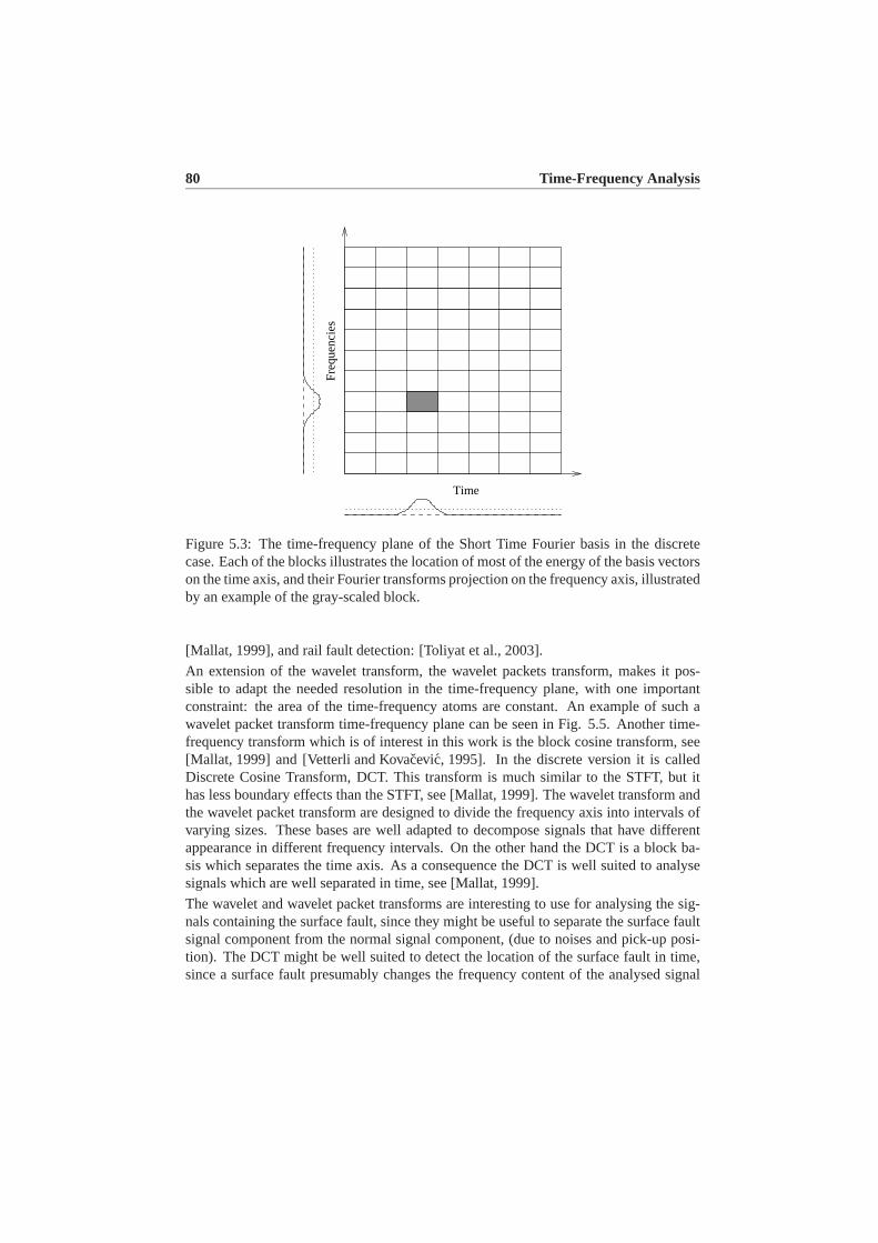
80 Time-Frequency Analysis
Time
Freq
uenc
ies
Figure 5.3: The time-frequency plane of the Short Time Fourier basis in the discretecase. Each of the blocks illustrates the location of most of the energy of the basis vectorson the time axis, and their Fourier transforms projection on the frequency axis, illustratedby an example of the gray-scaled block.
[Mallat, 1999], and rail fault detection: [Toliyat et al., 2003].
An extension of the wavelet transform, the wavelet packets transform, makes it pos-sible to adapt the needed resolution in the time-frequency plane, with one importantconstraint: the area of the time-frequency atoms are constant. An example of such awavelet packet transform time-frequency plane can be seen in Fig. 5.5. Another time-frequency transform which is of interest in this work is the block cosine transform, see[Mallat, 1999] and [Vetterli and Kovacevic, 1995]. In the discrete version it is calledDiscrete Cosine Transform, DCT. This transform is much similar to the STFT, but ithas less boundary effects than the STFT, see [Mallat, 1999]. The wavelet transform andthe wavelet packet transform are designed to divide the frequency axis into intervals ofvarying sizes. These bases are well adapted to decompose signals that have differentappearance in different frequency intervals. On the other hand the DCT is a block ba-sis which separates the time axis. As a consequence the DCT is well suited to analysesignals which are well separated in time, see [Mallat, 1999].
The wavelet and wavelet packet transforms are interesting to use for analysing the sig-nals containing the surface fault, since they might be useful to separate the surface faultsignal component from the normal signal component, (due to noises and pick-up posi-tion). The DCT might be well suited to detect the location of the surface fault in time,since a surface fault presumably changes the frequency content of the analysed signal

5.1 Motivation of different time-frequency bases 81
Time
Freq
uenc
ies
Figure 5.4: The time-frequency plane of a Wavelet basis in the discrete case. Each of theblocks illustrates the location of most of the energy of the basis vectors on the time axis,and their Fourier transforms projection on the frequency axis, illustrated by an exampleof the gray-scaled block.
Time
Freq
uenc
ies
Figure 5.5: Principle time-frequency plane of an example of a Wavelet packet basis inthe discrete case. Each of the blocks illustrates the location of majority of the energyof the basis vectors on the time axis, and their Fourier transforms projection on thefrequency axis, illustrated by an example of the gray-scaled block.

82 Time-Frequency Analysis
almost instantaneously.Another interesting basis for Time-Frequency based approximation of the surface faultsis the Karhunen-Loève basis. Given a set of signals, the Karhunen-Loève transformof this set is derived based on the set and minimises the average linear approximationerror, see [Mallat, 1999]. The Karhunen-Loève basis is related to the wavelet packetbasis in the way that if one finds the wavelet packet basis in a special way, it canbe proven that it is a fast computed approximation of the Karhunen-Loève basis, see[Wickerhauser, 1994a].In the following the four bases: wavelet, wavelet packet, discrete cosine and Karhunen-Loève, are described in more details, with the purpose of getting the reader to understandthe use of them in feature extraction of surface faults, which again is followed by adescription of the basis.
5.2 Wavelet basis
The wavelet basis is an orthogonal basis ofL2(R), which is formed by scalings andtranslations of the mother wavelet,Ψ(t) ∈ L2(R), with zero average:∫ +∞
−∞Ψ(t)dt = 0. (5.1)
The mother wavelet is normalised such that:∥∥Ψ
∥∥ = 1, and it is centred in the vicinityof t = 0. A family of orthogonal functions can be formed by scalingΨ with s andtranslating it byu
Ψu,s(t) =1√sΨ
(t − u
s
). (5.2)
These new functions do remain normalised as the mother wavelet. The wavelet trans-form of f ∈ L2(R) at timeu and scales is, see [Mallat, 1999]:
Wf(u, s) = 〈f,Ψu,s〉 =∫ +∞
−∞f(t)
1√(s)
Ψ∗(
t − u
s
)dt. (5.3)
Wf(u, s) is only known fors < s0 to recoverf a complement to the informationcorresponding toWf(u, s) is needed fors > s0. This is called the scaling function,Φthat is an aggregation of the mother wavelet at scale larger than 1, see [Mallat, 1999].The low frequent approximation off at the scale s is
Lf(u, s) = 〈f,Φu,s〉 =∫ +∞
−∞f(t)
1√(s)
Φ(
t − u
s
)dt. (5.4)
This continuous wavelet transform is computationally heavy to use, due to the integral,whereas the Discrete Wavelet Transform, DWT, can be implemented by the use of filterbanks. This transform is described and used by many authors, some examples on theseare: [Mallat, 1999], [Jensen and la Cour-Harbo, 2001], [Strang and Nguyen, 1997],[Vetterli and Kovacevic, 1995], [Wickerhauser, 1994a].
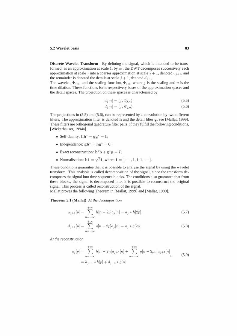
5.2 Wavelet basis 83
Discrete Wavelet Transform By defining the signal, which is intended to be trans-formed, as an approximation at scale 1, bya1, the DWT decomposes successively eachapproximation at scalej into a coarser approximation at scalej + 1, denotedaj+1, andthe remainder is denoted the details at scalej + 1, denoteddj+1.The wavelet,Ψj,n, and the scaling function,Φj,n, wherej is the scaling andn is thetime dilation. These functions form respectively bases of the approximation spaces andthe detail spaces. The projection on these spaces is characterised by
aj [n] = 〈f,Φj,n〉 (5.5)
dj [n] = 〈f,Ψj,n〉 . (5.6)
The projections in (5.5) and (5.6), can be represented by a convolution by two differentfilters. The approximation filter is denotedh and the detail filterg, see [Mallat, 1999].These filters are orthogonal quadrature filter pairs, if they fulfill the following conditions,[Wickerhauser, 1994a].
• Self-duality:hh∗ = gg∗ = I;
• Independence:gh∗ = hg∗ = 0;
• Exact reconstruction:h∗h + g∗g = I;
• Normalisation:h1 =√
21, where1 = {· · · , 1, 1, 1, · · · }.
These conditions guarantee that it is possible to analyse the signal by using the wavelettransform. This analysis is called decomposition of the signal, since the transform de-composes the signal into time sequence blocks. The conditions also guarantee that fromthese blocks, the signal is decomposed into, it is possible to reconstruct the originalsignal. This process is called reconstruction of the signal.Mallat proves the following Theorem in [Mallat, 1999] and [Mallat, 1989].
Theorem 5.1 (Mallat) At the decomposition
aj+1[p] =+∞∑
n=−∞h[n − 2p]aj [n] = aj ∗ h[2p], (5.7)
dj+1[p] =+∞∑
n=−∞g[n − 2p]aj [n] = aj ∗ g[2p]. (5.8)
At the reconstruction
aj [p] =+∞∑
n=−∞h[n − 2n]aj+1[n] +
+∞∑n=−∞
g[n − 2pn]aj+1[n]
= aj+1 ∗ h[p] + dj+1 ∗ g[p]
, (5.9)

84 Time-Frequency Analysis
↓ 2 ↓ 2
↓ 2 ↓ 2
aj
aj+1
aj+2
dj+1
dj+2
g
g
h
h
Figure 5.6: Illustration of the cascade filter implementation of the wavelet transform.his the low-pass filter andg is the low-pass filter.aj is the approximation at levelj, anddj is the details at levelj.
wherex[n] = x[−n] and x[n] =
{x[p] if n = 2p0 if n = 2p + 1
. Notice the summation goes
from −∞ to ∞ even though the filters and signals in practice are finite. The theoremis still valid with finite signals, but some boundary effects can occur if the boundariesare not handled in an optimal way. The cascade filtering implementation of the DWT isillustrated in Fig. 5.6. This cascade filtering can continue as long asaj can be decom-posed, which means that if one would like to decomposeaj , the length ofaj is requiredto be larger than 2.After this definition of the wavelet decomposition and reconstruction, some differentwavelets functions are investigated. The choice of the wavelet is of high importance inthe analysis of a signal. E.g. if the scope of an analysis is to detect a given signal com-ponent, it could be a scratch in the residuals. It is clearly a good idea to use a waveletthat has an appearance similar to the scratch. As a consequence of the importance ofthe wavelets on the achieved analysis results, there is defined a high number of differ-ent wavelets. In Fig. 5.7 the wavelet and scaling functions of the Daubechies 1-4 are
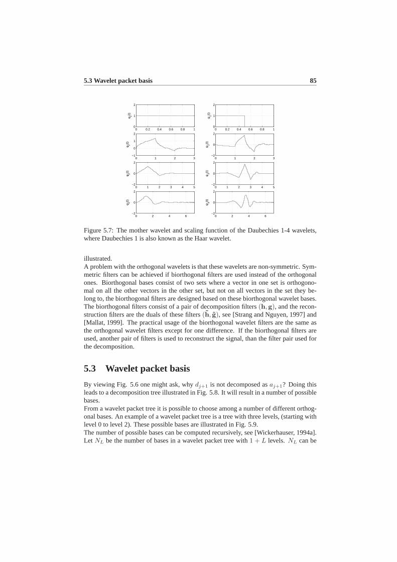
5.3 Wavelet packet basis 85
0 0.2 0.4 0.6 0.8 10
1
2
φ 1(t)
0 0.2 0.4 0.6 0.8 10
1
2
ψ1(t
)
0 1 2 3−1
0
1
2
φ 2(t)
0 1 2 3−2
0
2
ψ2(t
)
0 1 2 3 4 5−2
0
2
φ 3(t)
0 1 2 3 4 5−2
0
2
ψ3(t
)
0 2 4 6−2
0
2
φ 4(t)
0 2 4 6−2
0
2
ψ4(t
)
Figure 5.7: The mother wavelet and scaling function of the Daubechies 1-4 wavelets,where Daubechies 1 is also known as the Haar wavelet.
illustrated.A problem with the orthogonal wavelets is that these wavelets are non-symmetric. Sym-metric filters can be achieved if biorthogonal filters are used instead of the orthogonalones. Biorthogonal bases consist of two sets where a vector in one set is orthogono-mal on all the other vectors in the other set, but not on all vectors in the set they be-long to, the biorthogonal filters are designed based on these biorthogonal wavelet bases.The biorthogonal filters consist of a pair of decomposition filters(h,g), and the recon-struction filters are the duals of these filters(h, g), see [Strang and Nguyen, 1997] and[Mallat, 1999]. The practical usage of the biorthogonal wavelet filters are the same asthe orthogonal wavelet filters except for one difference. If the biorthogonal filters areused, another pair of filters is used to reconstruct the signal, than the filter pair used forthe decomposition.
5.3 Wavelet packet basis
By viewing Fig. 5.6 one might ask, whydj+1 is not decomposed asaj+1? Doing thisleads to a decomposition tree illustrated in Fig. 5.8. It will result in a number of possiblebases.From a wavelet packet tree it is possible to choose among a number of different orthog-onal bases. An example of a wavelet packet tree is a tree with three levels, (starting withlevel 0 to level 2). These possible bases are illustrated in Fig. 5.9.The number of possible bases can be computed recursively, see [Wickerhauser, 1994a].Let NL be the number of bases in a wavelet packet tree with1 + L levels. NL can be

86 Time-Frequency Analysis
↓ 2 ↓ 2
↓ 2 ↓ 2 ↓ 2 ↓ 2
aj
aj+1
aj+2,1 aj+2,1
dj+1
dj+2,1 dj+2,1
g
g g
h
h h
Figure 5.8: Illustration of the cascade filter implementation of the wavelet packet trans-form. h is the low-pass filter andg is the low-pass filter.aj is the approximation at levelj, anddj is the details at levelj.
computed recursively by the use of (5.10) and (5.11).
N0 = 1, (5.10)
and
NL+1 = 1 + N2L. (5.11)
A simple estimate ofNL+1 is NL+1 > 22L
for all L > 1, [Wickerhauser, 1994a]. Thenumber of possible bases for wavelet packet trees with 1-8 levels are shown in Table 5.1.These high numbers of possible bases for such small number of levels in the waveletpacket tree indicate the need for a fast algorithm to find the best basis in thewavelet packet tree, given a wavelet basis, information cost function and trainingsignal. The best basis search is such a method, see [Wickerhauser, 1994a] and[Coifman and Wickerhauser, 1992].

5.3 Wavelet packet basis 87
d)
b)
e)
c)
a)
Figure 5.9: Illustration of the possible basis of a wavelet packet tree of 3 levels. Thegray area illustrates the possible bases in the five wavelet packet trees. a) is the basis ofthe original signal, where b)-e) are the remaining four possible wavelet packet bases.
Number of levels in tree Number of possible bases1 12 23 54 265 6776 4583307 2100663889018 44127887745906175987802
Table 5.1: The number of possible bases in the wavelet packet tree for 1-8 levels, see[Jensen and la Cour-Harbo, 2001]

88 Time-Frequency Analysis
Best basis search The best basis obviously depends on the application of which itshould be found. In order to measure how suitable the basis is, an information costfunction is introduced. Such a cost function measures the cost of a given representation,where the best basis has the smallest cost. The cost function,K(·) must fulfill somespecific properties.
1. K(·) ∈ R2. K ([
v w])
= K(v) + K(w), for finite length vectorsv andw.
3. K(0) = 0.
Some of the commonly used information cost functions are: Number above a giventhreshold, Concentration inlp, Entropy, and Logarithm of energy.Having the information cost function in mind, it is possible to describe the best basissearch, [Wickerhauser, 1994a].
1. Compute the cost function of all elements in the wavelet packet tree, see Fig. 5.8.
2. Mark all elements on the bottom levelJ
3. Letj = J
4. Letk = 0
5. Compare the cost valuev1 of elementk, (counting from the left), on levelj − 1to the sumv2 of the cost values of the elements2k and2k + 1 on levelj.
(a) If v1 ≤ v2, all the marks below elementk on levelj − 1 is deleted, andelementk is marked.
(b) If v1 > v2, the cost valuev1 of elementk is replaced withv2.
6. k = k +1. If there are more elements on levelj(if k < 2j−1 − 1), jump to step 5.
7. j = j + 1. If j > 1, jump to step 4.
8. The marked basis has the lowest possible cost value. This value is fund at the topelement.
The best basis search algorithm is illustrated by an example, which can be found in Fig.5.10 where a signal of length 8 is decomposed, with the Haar basis, the decompositiontree can be seen in the top of the figure. Next the information cost function values arecomputed for all the elements, with the cost function: counting numbers in each elementbeing absolute larger than 1. The algorithm is carried out for this example in the lowerpart of the figure. The use of this algorithm ends up with a best basis representation ofthe original signal being:
[∣∣10 6 22 6∣∣ ∣∣−1
∣∣ ∣∣1∣∣ ∣∣3 3∣∣].

5.3 Wavelet packet basis 89
11
4
1
4
7
11 0 1
2 2 1 13)
7
4
6
−3
6 −6 −2
8 14 2 8 0 −2 6 0
11 5 −3 −1 1 6
1)
16 24
2)4
5)
5
4 1
1 1 1 1 0 0 1 1
10224)
7
0
0
−2
6
4)4)2
1 1 1 1 0 0 1 1
122
4 1
1 1 1 1 0 0 1 1
102
44 0 12 20 8
10 6 22
Figure 5.10: An illustration of the best basis search. The threshold above 1 is used ascost function and the Haar wavelet is the used wavelet, where 1) is the original waveletpacket tree, 2) is the computed informational costs, 3)-5) are the iterations in the bestbasis algorithm, ending up within a best basis representation of the signal being: [|10, 6,22, 6|,|-1|,|1|,|3, 3|]
This best basis is computed based on one signal, cost function and wavelet. One canchoose among the usable informational cost functions and wavelet bases. However,using only one signal to find the best basis is not always useful in practical applications.This can be illustrated by an example. The problem is to detect a given fault in a residual,N time sequences of measurements of this residual containing a fault is available. AlltheseN time sequences of measurement are probably not all alike. This means that itcould happen that the chosen signal for training the best basis, is a poor representationof other signals in the set of all the measured signals. It would be better to base the bestbasis search on more than one signal from the data set. Ideally the best basis searchshould be based on the entire data set.
Joint best basis The joint best basis is a method which takes the entire data set intoaccount when finding the best basis. The joint best basis search finds the best basisgiven a set of signals, of the same length. It could be a number of signals with the samefault. The joint best basis algorithm computes the jointly best bases given: the set ofsignals, an information cost function and a wavelet basis, see [Wickerhauser, 1994a],[Coifman and Wickerhauser, 1992] and [Saito, 1998]. The algorithm is as follows:
1. Compute the full wavelet packet tree of all the signals in the signal set.
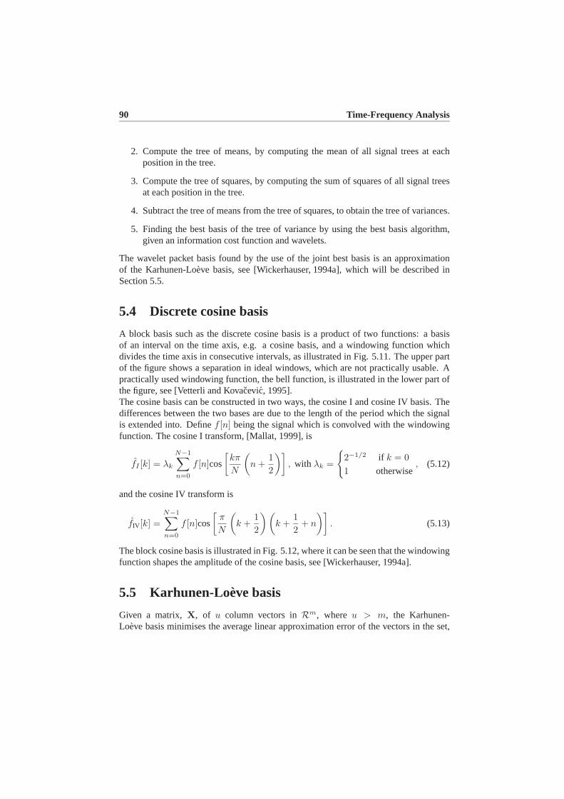
90 Time-Frequency Analysis
2. Compute the tree of means, by computing the mean of all signal trees at eachposition in the tree.
3. Compute the tree of squares, by computing the sum of squares of all signal treesat each position in the tree.
4. Subtract the tree of means from the tree of squares, to obtain the tree of variances.
5. Finding the best basis of the tree of variance by using the best basis algorithm,given an information cost function and wavelets.
The wavelet packet basis found by the use of the joint best basis is an approximationof the Karhunen-Loève basis, see [Wickerhauser, 1994a], which will be described inSection 5.5.
5.4 Discrete cosine basis
A block basis such as the discrete cosine basis is a product of two functions: a basisof an interval on the time axis, e.g. a cosine basis, and a windowing function whichdivides the time axis in consecutive intervals, as illustrated in Fig. 5.11. The upper partof the figure shows a separation in ideal windows, which are not practically usable. Apractically used windowing function, the bell function, is illustrated in the lower part ofthe figure, see [Vetterli and Kovacevic, 1995].The cosine basis can be constructed in two ways, the cosine I and cosine IV basis. Thedifferences between the two bases are due to the length of the period which the signalis extended into. Definef [n] being the signal which is convolved with the windowingfunction. The cosine I transform, [Mallat, 1999], is
fI [k] = λk
N−1∑n=0
f [n]cos
[kπ
N
(n +
12
)], with λk =
{2−1/2 if k = 01 otherwise
, (5.12)
and the cosine IV transform is
fIV [k] =N−1∑n=0
f [n]cos
[π
N
(k +
12
)(k +
12
+ n
)]. (5.13)
The block cosine basis is illustrated in Fig. 5.12, where it can be seen that the windowingfunction shapes the amplitude of the cosine basis, see [Wickerhauser, 1994a].
5.5 Karhunen-Loève basis
Given a matrix,X, of u column vectors inRm, where u > m, the Karhunen-Loève basis minimises the average linear approximation error of the vectors in the set,
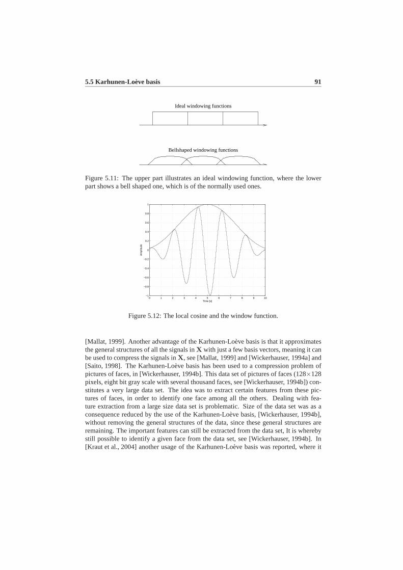
5.5 Karhunen-Loève basis 91
Ideal windowing functions
Bellshaped windowing functions
Figure 5.11: The upper part illustrates an ideal windowing function, where the lowerpart shows a bell shaped one, which is of the normally used ones.
0 1 2 3 4 5 6 7 8 9 10−1
−0.8
−0.6
−0.4
−0.2
0
0.2
0.4
0.6
0.8
1
Time [s]
Am
plitu
de
Figure 5.12: The local cosine and the window function.
[Mallat, 1999]. Another advantage of the Karhunen-Loève basis is that it approximatesthe general structures of all the signals inX with just a few basis vectors, meaning it canbe used to compress the signals inX, see [Mallat, 1999] and [Wickerhauser, 1994a] and[Saito, 1998]. The Karhunen-Loève basis has been used to a compression problem ofpictures of faces, in [Wickerhauser, 1994b]. This data set of pictures of faces (128×128pixels, eight bit gray scale with several thousand faces, see [Wickerhauser, 1994b]) con-stitutes a very large data set. The idea was to extract certain features from these pic-tures of faces, in order to identify one face among all the others. Dealing with fea-ture extraction from a large size data set is problematic. Size of the data set was as aconsequence reduced by the use of the Karhunen-Loève basis, [Wickerhauser, 1994b],without removing the general structures of the data, since these general structures areremaining. The important features can still be extracted from the data set, It is wherebystill possible to identify a given face from the data set, see [Wickerhauser, 1994b]. In[Kraut et al., 2004] another usage of the Karhunen-Loève basis was reported, where it

92 Time-Frequency Analysis
was used for efficient estimations of tropospheric refractivity using radar clutter.The Karhunen-Loève basis is computed based onX, first of all it is assumed that thecolumn vectors inX has zero mean, if not a preliminary step is introduced in order tofulfill that assumption. The Karhunen-Loève basis,K, can be defined as
K = {v1, · · · , vm}, (5.14)
is an orthornomal basis of eigenvectors of the matrixXXT , ordered in such a way thatvn is associated with the eigenvectorλn, andλi ≥ λj for i > j. A matrix of the basisvectors can following be defined as
KL =[vm, vm−1, · · · , vi
](5.15)
So in other words the Karhunen-Loève basis is the eigen vectors of the autocorrelationof X. The eigenvalues of the autocorrelation have the values of the variances of therelated Karhunen-Loève basis vectors. The approximating properties of the Karhunen-Loève basis vectors are sorted in increasing order, that means that if the basis consistsof p vectors the basis vectorp is the most approximating basis vector. In addition thegeneral structures in all the vectors inX are represented by only a few basis vectors.The remaining basis vectors represent the signal parts which are not general forX, i.e.noises in the signal, etc.It can be proven that
X = KlΣLl , (5.16)
where
Σ =[Σ 00 0
], (5.17)
Σ = diagonal(σ1, · · · , σp), (5.18)
σ1 ≥ σ2 ≥ · · · ≥ σp ≥ 0, (5.19)
andLl is a unitary matrix. From this it can clearly be seen that this decomposition is theSingular Value Decomposition.
5.6 Summary
In this chapter the necessary back-ground theory in the field of time-frequency analysishas been described, starting with a general description of the field of time-frequencyanalysis, see Section 5.1. This is followed by the description of four different interestingbases. The wavelet basis is described in Section 5.2, and the wavelet packet basis isdescribed in Section 5.3, where both the best basis search and the joint best basis searchare described. The discrete cosine basis is described in Section 5.4, which describesboth DCT-I and DCT-IV. The Karhunen-Loève basis is described in Section 5.5.

Chapter 6
Time Localisation of the SurfaceFaults
After the introduction to time-frequency based bases in Chapter 5, and the construc-tion of decoupled residuals in Chapter 4, the increased fault detection powers of theseresiduals have been illustrated in Section 4.4. These bases can be useful in the timelocalisation of the surface faults. The time location of the surface faults is found basedon analysis of the residualsαf [n] andαr[n]. The next problem is to locate the surfacefaults (fault detection) in time based on the residuals. Thresholding is often used to de-tect and locate the fault in the residual. [Basseville and Nikiforov, 1993] present meth-ods to compute the thresholds based on statistical information. Schneiders has usedwavelet analysis to detect surface faults in optical disc players, see [Schneiders, 2001]as well as [Goossens and Odgaard, 2003], however, inpsecting these one can come tothe conclusion that it would be better to use wavelet packet fitlers instead. In this chap-ter some other methods are used: detection of frequency change, extended thresholding,and wavelet packet filters.However, before these fault time localisation methods are described, some online com-putational remarks are given regarding the application, see Section 6.1.The frequency content of the residuals change during surface faults. This makes it obvi-ous to use a method to detect and locate the fault, which is based on time-frequencyanalysis, instead of the statistics of the residuals with and without faults. A time-frequency based method in this case might be able to detect the beginning of a faultfrom the background noise. This detection of the change in frequency content is simi-lar to the vocal segmentation problem described in [Wesfreid and Wickerhauser, 1999],where Fang’s algorithm for segmentation of the time axis was used, [Fang, 1994] and[Wesfreid and Wickerhauser, 1999]. This method is described in Section 6.2On the other hand if a thresholding method is used, see Section 6.3, it needs to be adaptedto some applicational problems. Some additional problems are encountered when sur-
93

94 Time Localisation of the Surface Faults
face faults shall be detected. Signal noises are different from one disc to another, as aconsequence the thresholds need to be adapted to the given noise level. The skewness ofthe disc influences the residuals by changing the received fraction of energy in the OPU.This eccentricity part is mainly due to the angular velocity of the CD-player, which re-sults in a low frequent component in the residuals. It is also important to have a goodlocalisation of the beginning and end of the faults. From experiences it is known thata poor fault localisation can result in severe problems for the controllers. Finally, it isof high importance to avoid false positive detections of faults, since the fault accommo-dation will somehow make the controllers non sensible to the frequency content of thefaults. This means that the controllers cannot suppress disturbances in that frequencyrange during a detection of a fault. A consequence of that is that the time duration of thefault accommodation shall be reduced as much as possible.The final method used to locate the fault in time, see Section 6.4, is wavelet packet filtersdesigned partly based on the joint best basis search, where the best wavelet packet basisis found, based on a training set of measurements of real surface faults.
6.1 Online computation
It is problematic to use advanced signal processing online in a control system, sinceoutput of this signal processing is required at the time the fault is occurring. However,a surface fault such as a scratch has only small variations from an encounter to the nextencounter, this is due to the small distance from track to track, (the distance is only 1.6[µm]). This fact has been validated by experimental work, in [Odgaard et al., 2004d].βf [n], (the focus fault parameter, see (3.59)), of some sequently following encountersof a fault were plotted, and this plot clearly validates the point that a fault has a smallvariation from encounter to encounter. This can be seen from Fig. 6.1 and Fig. 4.2.This means the time-location and features extracted from the surface fault at an en-counter can be used when the same fault is occurring again at the next encounter. I.e.notice the two following important remarks: first of all the computations in the featureextraction can be spread out in longer time period and thereby make use of more ad-vanced algorithms possible, since these algorithms are too computationally demandingto compute them at once. It is at least important to have the entire fault available whenthe time-location and features are extracted. It would be difficult, if not to say impossi-ble to extract the frequency content of a fault based on just a few samples, or to classifythe fault based on a couple of samples. It is a requirement that the time-location and fea-tures are instantly available if they are used to handle the faults in a closed loop controlscheme. This can guaranteed if the time localisation from the last encounter of the faultis used together with a prediction of the length of one revolution.Even though surface faults have small variations from encounter to encounter they dovary over a larger number of encounters. This means that surface faults are small in thebeginning and being no problem to handle by the nominal controller, and develop over alarge number of tracks to be a large fault, which is problematic to handle by the nominal

6.2 Time localisation based on Fang’s segmentation 95
0 50 100 150 200 250 3000.8
0.85
0.9
0.95
1
1.05
1.1
1.15
Samples [n]
β f
Figure 6.1: βf [n] of a small scratch from a number of encounters of the same fault.Notice the small variation from encounter to encounter.
controller. Some experimental works could indicate that many scratches have an eyeshape, as illustrated in Fig. 6.2.To validate this eye shape, a 3-dimensional plot of a scratch on a disc is plotted in Fig.4.1.In this figureβf [n] is plotted with a number of sequential following fault encounters, thedepth and duration of the fault increase from encounter number 1 to the last encounter.
6.2 Time localisation based on Fang’s segmentation
Fang’s algorithm, [Fang, 1994], has not been published by its inventor, but it has beenpresented by other authors e.g. [Wesfreid and Wickerhauser, 1999]. This algorithm iswell suited to locate changes in the frequency content of a signal. This algorithm consistsof three parts:
• The instantaneous frequency change function at a given sample,n, IFC(n).
• An averaged frequency change function at the sample,n, AFC(n) which is anaveraged version ofIFC(n).
• A locator of the change in frequencies. The change in frequencies can be locatedby finding local extrema in theAFC(n) signal.
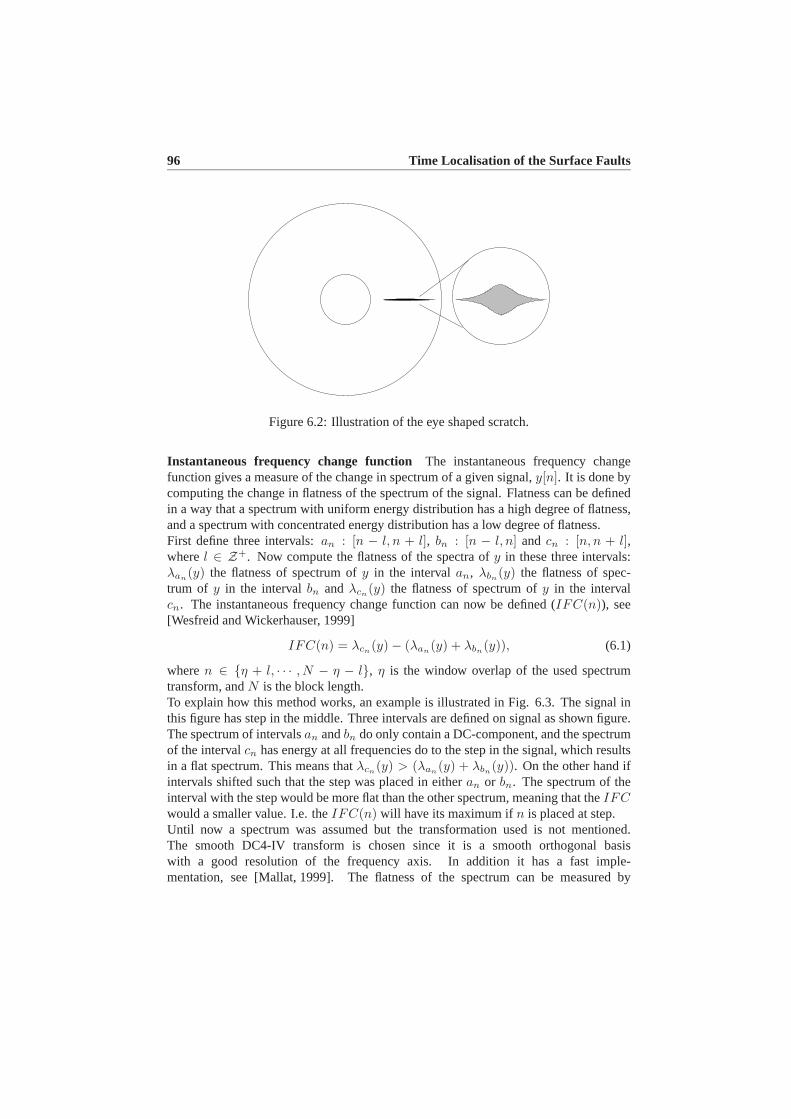
96 Time Localisation of the Surface Faults
Figure 6.2: Illustration of the eye shaped scratch.
Instantaneous frequency change function The instantaneous frequency changefunction gives a measure of the change in spectrum of a given signal,y[n]. It is done bycomputing the change in flatness of the spectrum of the signal. Flatness can be definedin a way that a spectrum with uniform energy distribution has a high degree of flatness,and a spectrum with concentrated energy distribution has a low degree of flatness.First define three intervals:an : [n − l, n + l], bn : [n − l, n] and cn : [n, n + l],wherel ∈ Z+. Now compute the flatness of the spectra ofy in these three intervals:λan
(y) the flatness of spectrum ofy in the intervalan, λbn(y) the flatness of spec-
trum of y in the intervalbn andλcn(y) the flatness of spectrum ofy in the interval
cn. The instantaneous frequency change function can now be defined (IFC(n)), see[Wesfreid and Wickerhauser, 1999]
IFC(n) = λcn(y) − (λan
(y) + λbn(y)), (6.1)
wheren ∈ {η + l, · · · , N − η − l}, η is the window overlap of the used spectrumtransform, andN is the block length.To explain how this method works, an example is illustrated in Fig. 6.3. The signal inthis figure has step in the middle. Three intervals are defined on signal as shown figure.The spectrum of intervalsan andbn do only contain a DC-component, and the spectrumof the intervalcn has energy at all frequencies do to the step in the signal, which resultsin a flat spectrum. This means thatλcn
(y) > (λan(y) + λbn
(y)). On the other hand ifintervals shifted such that the step was placed in eitheran or bn. The spectrum of theinterval with the step would be more flat than the other spectrum, meaning that theIFCwould a smaller value. I.e. theIFC(n) will have its maximum ifn is placed at step.Until now a spectrum was assumed but the transformation used is not mentioned.The smooth DC4-IV transform is chosen since it is a smooth orthogonal basiswith a good resolution of the frequency axis. In addition it has a fast imple-mentation, see [Mallat, 1999]. The flatness of the spectrum can be measured by
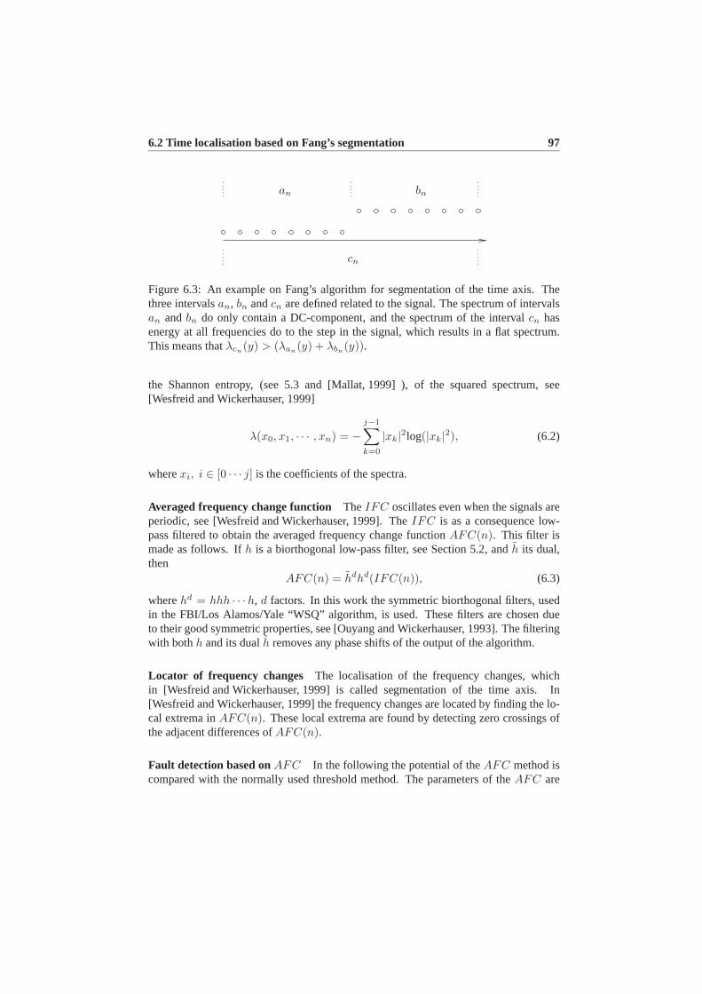
6.2 Time localisation based on Fang’s segmentation 97
an bn
cn
Figure 6.3: An example on Fang’s algorithm for segmentation of the time axis. Thethree intervalsan, bn andcn are defined related to the signal. The spectrum of intervalsan andbn do only contain a DC-component, and the spectrum of the intervalcn hasenergy at all frequencies do to the step in the signal, which results in a flat spectrum.This means thatλcn
(y) > (λan(y) + λbn
(y)).
the Shannon entropy, (see 5.3 and [Mallat, 1999] ), of the squared spectrum, see[Wesfreid and Wickerhauser, 1999]
λ(x0, x1, · · · , xn) = −j−1∑k=0
|xk|2log(|xk|2), (6.2)
wherexi, i ∈ [0 · · · j] is the coefficients of the spectra.
Averaged frequency change function TheIFC oscillates even when the signals areperiodic, see [Wesfreid and Wickerhauser, 1999]. TheIFC is as a consequence low-pass filtered to obtain the averaged frequency change functionAFC(n). This filter ismade as follows. Ifh is a biorthogonal low-pass filter, see Section 5.2, andh its dual,then
AFC(n) = hdhd(IFC(n)), (6.3)
wherehd = hhh · · ·h, d factors. In this work the symmetric biorthogonal filters, usedin the FBI/Los Alamos/Yale “WSQ” algorithm, is used. These filters are chosen dueto their good symmetric properties, see [Ouyang and Wickerhauser, 1993]. The filteringwith bothh and its dualh removes any phase shifts of the output of the algorithm.
Locator of frequency changes The localisation of the frequency changes, whichin [Wesfreid and Wickerhauser, 1999] is called segmentation of the time axis. In[Wesfreid and Wickerhauser, 1999] the frequency changes are located by finding the lo-cal extrema inAFC(n). These local extrema are found by detecting zero crossings ofthe adjacent differences ofAFC(n).
Fault detection based onAFC In the following the potential of theAFC method iscompared with the normally used threshold method. The parameters of theAFC are

98 Time Localisation of the Surface Faults
found by iterations, in a way that filters are focused on the changes in the frequencycontent of the fault, and not on the general frequency content of the signal. The usedparameters are:η = 16, l = 32 andd = 4. The two first parameters primarily determinethe location of the frequency region and the last parameter determines the width of thisfrequency change detection.The comparison of the algorithms is done by using computed residuals from three datasequences with representative faults, see Figs. 6.4-6.6.
2.658 2.659 2.66 2.661 2.662 2.663 2.664 2.665 2.666 2.667
x 104
−0.02
0
0.02
0.04
0.06
0.08
(a) The residual with first fault.
2.658 2.659 2.66 2.661 2.662 2.663 2.664 2.665 2.666 2.667 2.668
x 104
−2.78
−2.76
−2.74
−2.72
−2.7
−2.68
−2.66
−2.64
−2.62
−2.6x 10
−3
Sample [n]
AF
C(n
)
Begining
End
(b) TheAFC(n) of the residual with the firstfault.
Figure 6.4: An illustration of the first fault in the residual and theAFC(n) of the re-sidual. The abscissis is in samples. Note the markings of the beginning and end of thescratch. These locations of the beginning and the end of the fault based onAFC(n) arevery suitable.
By inspection it can be seen that finding the local minima, (due to a sign differencecompared with the original algorithm), of theAFC in Fig. 6.4(b), gives very goodindication of the beginning and end of the fault illustrated in Fig. 6.4(a). It is also seenthat theAFC in Fig. 6.5(b) cannot be used to locate the start and end of the fault,since its minimum does not locate the beginning and end of the fault. This means thatthe change in frequencies in the signal is not measured by theAFC function since thefrequencies changing are not in the interval of frequencies for which the algorithm isdesigned to measure changes. Instead, theAFC in this example looks like a low-passversion of the residual itself, and could be time located by the use of a simple thresholdmethod. On the other hand if the design is based on the fault in Fig. 6.5(a), it results in adesign which cannot be used to detect the beginning and end of the fault in Figs. 6.4(a)and 6.6(a). A design based on the fault in Fig. 6.6(a) was also tried, with the result thatit was well suited to locate the fault in Fig. 6.6(a) but not the fault in Figs. 6.5(a) and

6.2 Time localisation based on Fang’s segmentation 99
2.47 2.48 2.49 2.5 2.51 2.52 2.53
x 104
−0.04
−0.02
0
0.02
0.04
0.06
0.08
0.1
0.12
0.14
(a) The residual with second fault.
2.46 2.47 2.48 2.49 2.5 2.51 2.52 2.53 2.54
x 104
−3.4
−3.2
−3
−2.8
−2.6
−2.4
−2.2
x 10−3
(b) TheAFC(n) of the residual with the sec-ond fault.
Figure 6.5: An illustration of the second fault in the residual and theAFC(n) of theresidual. The abscissis is in samples. Note the lack of markings of the beginning andend of the scratch. This means that thisAFC(n) cannot be used to locate the faults intime.
2.592 2.594 2.596 2.598 2.6 2.602 2.604 2.606 2.608
x 104
−0.05
0
0.05
0.1
0.15
0.2
(a) The residual with third fault.
2.59 2.592 2.594 2.596 2.598 2.6 2.602 2.604 2.606 2.608 2.61
x 104
−3.05
−3
−2.95
−2.9
−2.85
−2.8
−2.75
−2.7
−2.65
−2.6x 10
−3
Sample [n]
AF
C(n
)
Begining
(b) TheAFC(n) of the residual with the thirdfault.
Figure 6.6: An illustration of the third fault in the residual and theAFC(n) of theresidual. The abscissis is in samples. Note the markings of the beginning of the scratch.TheAFC(n) can in this example only be used to locate the beginning and not the endof the fault and is as a consequence not usable in the given situation.

100 Time Localisation of the Surface Faults
6.4(a). The last example, Fig. 6.6(a), looks like the first one, Fig. 6.4(a), but theAFCof this signal has only one minimum, see Fig. 6.6(b), even though this minimum locatesthe start of the fault, this signal cannot be used to detect the end of it, since there is onlyone extrema in this signal.This means that using theAFC of the residuals in some cases gives a much better timelocalisation of the fault than by using thresholds since the thresholds have to be largerthan the signal noise. As a consequence the beginning of the fault cannot be localisedwell. TheAFC of the first fault seems to do exactly this. Unfortunately it does nothave the same good results in the other examples, for the second example, see Fig.6.5(a). TheAFC looks like a low-pass filtered version of the original example. Thefault could be located by using a threshold. However, the DCT used in theAFC isa computationally demanding algorithm. The design of theAFC algorithm results inan over trained filter, which is too narrow banded to localise other surface faults. Thisproblem is also mentioned in [Ye et al., 2004] and [Ye et al., 2003], where too narrowbanded parity filters used for fault detection results in a high level of non-detections.One way to use this method for time localisation of faults is to use a previous classifi-cation of the faults, and adapt a number ofAFC filters to the different classes of faults.This is usable since the faults slowly but steadily are evolved for each revolution of thedisc from being no problem to handle to be a problem, meaning it is possible to classifythe fault before using theAFC filters to locate the fault in time.
Summary of time localisation by the use of Fang’s algorithm This means that eventhough there is a clear potential of theAFC based detection for some faults see Fig.6.4(a), it do not shows the same good potentials in situations like in Fig. 6.5(a). Itcannot be concluded that using oneAFC filter is recommendable in general for timelocalisation of surface faults on optical discs, since the required filters are too narrowbanded for locating all the surface faults. A strategy could be to implement a numberof AFC filters, where each is adapted to a given class of faults. This strategy wouldprobably have an improved time localisation of the surface faults, but would require ahigh amount of computations.
6.3 Cleaning of residuals and extended threshold
Cleaning of residuals Skew discs introduces a problem if thresholds are used for thetime localisation of the surface fault. The skewness of the disc results in oscillatingreferences to the focus and radial distances, which are handled by the controllers. Theused residuals are designed in a way such that they should be decoupled from these dis-tances. However, in addition to these variations the skewness also results in oscillationsin the received amount of energy at the detectors. This can be seen as oscillations in theresidualsαf [n] andαr[n]. The skewness is illustrated in Fig. 6.8, from this figure it isseen that a skew disc does not reflect all the light back to the OPU. A couple of residualswith a clear skewness problem is illustrated by an example from a disc with a scratch
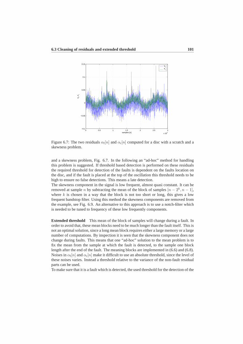
6.3 Cleaning of residuals and extended threshold 101
0 0.5 1 1.5 2 2.5 3
x 104
−0.1
−0.05
0
0.05
0.1
0.15
samples [n]
α f, αr
αf
αr
Figure 6.7: The two residualsαf [n] andαr[n] computed for a disc with a scratch and askewness problem.
and a skewness problem, Fig. 6.7. In the following an “ad-hoc” method for handlingthis problem is suggested. If threshold based detection is performed on these residualsthe required threshold for detection of the faults is dependent on the faults location onthe disc, and if the fault is placed at the top of the oscillation this threshold needs to behigh to ensure no false detections. This means a late detection.The skewness component in the signal is low frequent, almost quasi constant. It can beremoved at samplen by subtracting the mean of the block of samples[n − 2k, n − 1],wherek is chosen in a way that the block is not too short or long, this gives a lowfrequent bandstop filter. Using this method the skewness components are removed fromthe example, see Fig. 6.9. An alternative to this approach is to use a notch-filter whichis needed to be tuned to frequency of these low frequently components.
Extended threshold This mean of the block of samples will change during a fault. Inorder to avoid that, these mean blocks need to be much longer than the fault itself. This isnot an optimal solution, since a long mean block requires either a large memory or a largenumber of computations. By inspection it is seen that the skewness component does notchange during faults. This means that one “ad-hoc” solution to the mean problem is tofix the mean from the sample at which the fault is detected, to the sample one blocklength after the end of the fault. The meaning blocks are implemented in (6.6) and (6.8).Noises inαf [n] andαr[n] make it difficult to use an absolute threshold, since the level ofthese noises varies. Instead a threshold relative to the variance of the non-fault residualparts can be used.To make sure that it is a fault which is detected, the used threshold for the detection of the

102 Time Localisation of the Surface Faults
OPU
ef
Figure 6.8: Illustration of the skewness of the disc. Notice that not all the reflected lightreaches the OPU.
0 0.5 1 1.5 2 2.5 3
x 104
−0.1
−0.05
0
0.05
0.1
0.15
samples [n]
α f, αr
αf
αr
Figure 6.9: The skewness component is removed from the two residualsαf [n] andαr[n]computed for a disc with a scratch and a skewness problem.
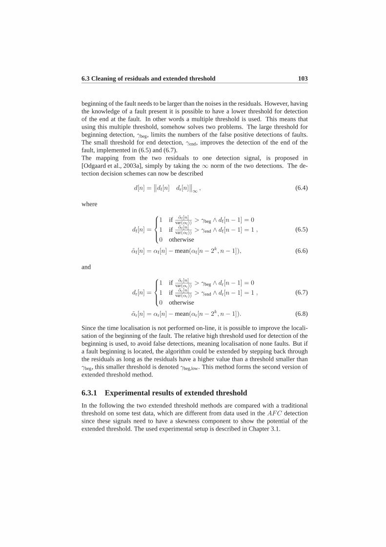
6.3 Cleaning of residuals and extended threshold 103
beginning of the fault needs to be larger than the noises in the residuals. However, havingthe knowledge of a fault present it is possible to have a lower threshold for detectionof the end at the fault. In other words a multiple threshold is used. This means thatusing this multiple threshold, somehow solves two problems. The large threshold forbeginning detection,γbeg, limits the numbers of the false positive detections of faults.The small threshold for end detection,γend, improves the detection of the end of thefault, implemented in (6.5) and (6.7).The mapping from the two residuals to one detection signal, is proposed in[Odgaard et al., 2003a], simply by taking the∞ norm of the two detections. The de-tection decision schemes can now be described
d[n] =∥∥df [n] dr[n]
∥∥∞ , (6.4)
where
df [n] =
1 if αf [n]var(αf))
> γbeg∧ df [n − 1] = 0
1 if αf [n]var(αf))
> γend∧ df [n − 1] = 1
0 otherwise
, (6.5)
αf [n] = αf [n] − mean(αf [n − 2k, n − 1]), (6.6)
and
dr[n] =
1 if αr[n]var(αr))
> γbeg∧ dr[n − 1] = 0
1 if αr[n]var(αr))
> γend∧ dr[n − 1] = 1
0 otherwise
, (6.7)
αr[n] = αr[n] − mean(αr[n − 2k, n − 1]). (6.8)
Since the time localisation is not performed on-line, it is possible to improve the locali-sation of the beginning of the fault. The relative high threshold used for detection of thebeginning is used, to avoid false detections, meaning localisation of none faults. But ifa fault beginning is located, the algorithm could be extended by stepping back throughthe residuals as long as the residuals have a higher value than a threshold smaller thanγbeg, this smaller threshold is denotedγbeg,low. This method forms the second version ofextended threshold method.
6.3.1 Experimental results of extended threshold
In the following the two extended threshold methods are compared with a traditionalthreshold on some test data, which are different from data used in theAFC detectionsince these signals need to have a skewness component to show the potential of theextended threshold. The used experimental setup is described in Chapter 3.1.

104 Time Localisation of the Surface Faults
0 0.5 1 1.5 2 2.5 3
x 104
−0.1
−0.05
0
0.05
0.1
0.15
0.2
0.25
samples [n]
α f
0 0.5 1 1.5 2 2.5 3
x 104
−0.1
−0.05
0
0.05
0.1
0.15
0.2
0.25
samples [n]
α r
Figure 6.10:αf [n] andαr[n] computed of sampled signals with surface faults and eccen-tricity problems.
Results on the extended threshold method Residuals of the test data are presentedin Fig. 6.10.Both the simple and the extended threshold methods were used for four different faultsin the residuals illustrated in Fig. 6.10. The thresholds are found such that false positivedetections are avoided, meaning that standard and first extended version methods shouldgive almost the same beginning detection but both extended methods should give a betterdetection of the end of the fault, and the second version of the extended method shouldalso improve the localisation of the beginning of the fault. The results are shown inTable 6.1. From the results in Table 6.1 it can be seen that both extended thresholdmethods perform better in the localisation of the end of the faults, which is expecteddue to the multiple thresholds. The second version of the extended threshold methoddoes also improve the localisation of the beginning of the fault, whereas the first versionof the extended method performs as well as the normal threshold. The potential ofthe extended method regarding removal of the eccentricity is only revealed in the lastexample. In this example both extended methods localise the beginning and end of thefault based onαf [n] close to the beginning found by inspection. The normal thresholdmethod has a larger general locating error.
6.3.2 Summary of time localisation by extended threshold
The threshold method is extended to improve its handling of disc eccentricity and touse multiple thresholds, meaning that one is used for detection at the beginning and asmaller one is used for detection at the end. This gives a better time localisation at the

6.4 Wavelet packet based time-localisation of the surface faults 105
αf , αr Inspection Normal Extended v.1 Extended v.2
αf 2830-2870 2843-2865 2844-2867 2833-2867αr 2830-2870 2837-2863 2837-2870 2834-2870
αf 6752-6780 6754-6776 6754-6778 6754-6778αr 6752-6780 6757-6773 6757-6775 6755-6775
αf 13202-13227 13204-13223 13204-13227 13203-13227αr 13202-13227 13205-13222 13205-13224 13204-13224
αf 13424-13470 13445-13465 13427-13469 13426-13469αr 13424-13470 13446-13464 13446-13465 13445-13465
Table 6.1: The four examples of the time localisation based on the two threshold meth-ods, and the localisation by visual inspection.
end of the surface fault. Since the time localisation of the faults is performed off-line,the second version of the extended threshold is implemented by using a small beginningthreshold, if a fault has been located.
6.4 Wavelet packet based time-localisation of the sur-face faults
It might be a good idea to use the wavelet and wavelet packet bases to locate thesurface faults in time. This has been done, e.g. see [Schneiders, 2001], who useswavelets to detect the surface faults, and in a different setup, the DVD-player, a waveletpacket based method is used for fault detection, which in principle is time localisa-tion of the fault. This fault detection is a part of method to handle surface faults, see[Goossens and Odgaard, 2003]. Both methods are based on the normally used residuals,(the sum signals) and not the decoupled residuals derived in this thesis. The wavelet andwavelet packet filters designed in [Schneiders, 2001] and [Goossens and Odgaard, 2003]are based on only one training signal. This can result in a problem. If another fault isapplied to the filter it does clearly not detect this fault as well as the surface fault usedfor the design of the filter.This over-training to the faults in the training set results in wavelet filters which havea too narrow-pass band, meaning that the main energy of the other faults are outsidethe pass band of the designed wavelet filters. This is more or less the same conclusionobtained in [Ye et al., 2004] and [Ye et al., 2003], where it is concluded that a too narrowbanded filter used for fault detection results in a clear increase in the non detected faults.This problem of designing a wavelet packet filter to detect surface faults which is notentirely alike, can be handled better by using the joint best basis search, instead of thebest basis search, which only finds the best basis given one signal and not a number of

106 Time Localisation of the Surface Faults
signals.
Training data From the focus and radial residuals,αf [n] andαr[n], faults are extractedbased on the algorithm described in [Odgaard and Wickerhauser, 2004]. Each detectedfault is extracted into a column vector with the length of 256=28 samples. This lengthis chosen since all faults in the dataset are shorter than 256 samples. The faults areextracted with symmetric geometric centre intended to be in the middle of the faultvector. Each vector can contain several faults (especially fingerprints). In addition thecentralisation is not totally successfully due to implementation. It was chosen that agiven fault is only contained in one fault vector. I.e. the centre is not always in themiddle of the vectors.This extraction gives two matrices with faults. The faults inαf [n] are collected inFf
and the faults inαr[n] are collected inFr, where each column in the matrices is a faultvector.
Joint best basis A joint best basis is following found forFf and Fr, where somedifferent wavelets also are tried. The problem in using the joint best basis algorithmdirectly is the choice of information cost function and the best basis search. Then usedto fault detection, the scope is to find a band-pass filter which separates the surface faultfrom the background noises in the residuals. Instead, a heuristic based method is used.The method takes its starting point in the tree of variances, used in the joint best basisalgorithm, see [Odgaard et al., 2004e]. The used method consists of the following steps:
1. Compute the tree of variances.
2. Search down the levels in the tree to find a level where the approximations anddetails both contain energy.
3. Use these details for the fault detection.
This method is following used onαf [n] andαr[n]. Starting withαf [n], the Haar waveletis used, since it is well suited for detection changes in the signal, and is short. By usingthe heuristic method, the interesting part of the tree of variance can be seen in Fig. 6.11.The figure starts with the original signal. The remaining figure parts are located bydenoting a low-pass filtering withh and high-pass filtering withg, meaning that twolow-pass filterings followed by one high-pass, are denotedhhg. The second plot ish,the third ishh, the fourth ishhh, the fifth ishhhh and the last one ishhhg. Noticethe large change fromhhh to hhhh, which results in a significant signal inhhhg. Thissignal is useful for fault detection, since it has relatively large signal parts, and does notcontain the near zero frequencies, where disturbances are dominating.This means that a useful filter for fault detection inαf [n] is found. It is three Haar lowpass filters followed by one Haar high-pass filter. The frequency amplitude plot of thisfilter is illustrated in Fig. 6.12.

6.4 Wavelet packet based time-localisation of the surface faults 107
0 50 100 150 200 250 3000
0.05
α f
0 20 40 60 80 100 120 1400
0.02
0.04a 1
0 10 20 30 40 50 60 700
0.02
0.04
a 2
0 5 10 15 20 25 30 350
0.05
a 3
0 2 4 6 8 10 12 14 160
0.05
0.1
a 4
0 2 4 6 8 10 12 14 160
0.02
0.04
d 4
Figure 6.11: The part of the tree of variance ofαf [n], which is interesting in the usedmethod. The figure starts with the original signal. The remaining figure parts are locatedby denoting a low-pass filtering withh and high-pass filtering withh, meaning that twolow-pass filterings followed by one high-pass, are denotedhhg. The second plot ish,the third ishh, the fourth ishhh, the fifth ishhhh and the last one ishhhg.
0 0.5 1 1.5 2 2.5 3 3.5 4
x 104
−100
−80
−60
−40
−20
0
20
Frequency [Hz]
Am
plitu
de
Figure 6.12: The frequency amplitude plot of filter consisting of three times Haar low-pass filtering followed by one time Haar high-pass filtering.
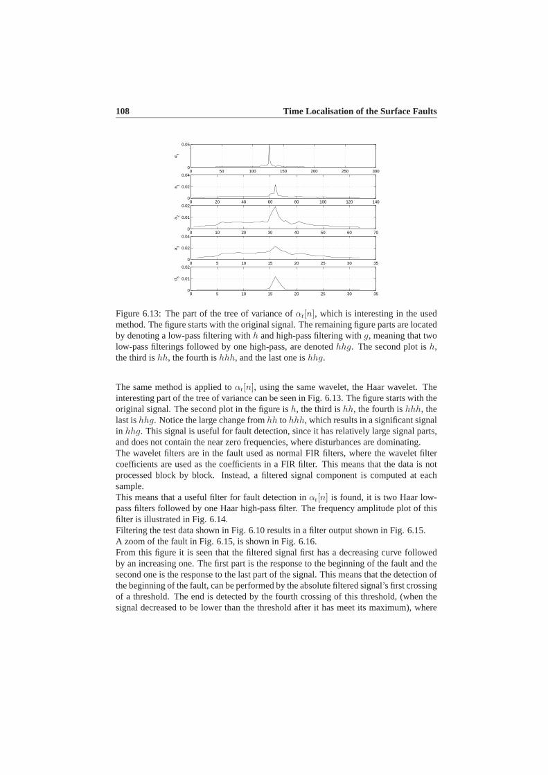
108 Time Localisation of the Surface Faults
0 50 100 150 200 250 3000
0.05
α f
0 20 40 60 80 100 120 1400
0.02
0.04a 1
0 10 20 30 40 50 60 700
0.01
0.02
a 2
0 5 10 15 20 25 30 350
0.02
0.04
a 3
0 5 10 15 20 25 30 350
0.01
0.02
d 3
Figure 6.13: The part of the tree of variance ofαr[n], which is interesting in the usedmethod. The figure starts with the original signal. The remaining figure parts are locatedby denoting a low-pass filtering withh and high-pass filtering withg, meaning that twolow-pass filterings followed by one high-pass, are denotedhhg. The second plot ish,the third ishh, the fourth ishhh, and the last one ishhg.
The same method is applied toαr[n], using the same wavelet, the Haar wavelet. Theinteresting part of the tree of variance can be seen in Fig. 6.13. The figure starts with theoriginal signal. The second plot in the figure ish, the third ishh, the fourth ishhh, thelast ishhg. Notice the large change fromhh to hhh, which results in a significant signalin hhg. This signal is useful for fault detection, since it has relatively large signal parts,and does not contain the near zero frequencies, where disturbances are dominating.The wavelet filters are in the fault used as normal FIR filters, where the wavelet filtercoefficients are used as the coefficients in a FIR filter. This means that the data is notprocessed block by block. Instead, a filtered signal component is computed at eachsample.This means that a useful filter for fault detection inαr[n] is found, it is two Haar low-pass filters followed by one Haar high-pass filter. The frequency amplitude plot of thisfilter is illustrated in Fig. 6.14.Filtering the test data shown in Fig. 6.10 results in a filter output shown in Fig. 6.15.A zoom of the fault in Fig. 6.15, is shown in Fig. 6.16.From this figure it is seen that the filtered signal first has a decreasing curve followedby an increasing one. The first part is the response to the beginning of the fault and thesecond one is the response to the last part of the signal. This means that the detection ofthe beginning of the fault, can be performed by the absolute filtered signal’s first crossingof a threshold. The end is detected by the fourth crossing of this threshold, (when thesignal decreased to be lower than the threshold after it has meet its maximum), where
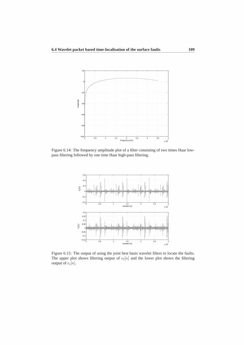
6.4 Wavelet packet based time-localisation of the surface faults 109
0 0.5 1 1.5 2 2.5 3 3.5 4
x 104
−100
−80
−60
−40
−20
0
20
Frequency [Hz]
Am
plitu
de
Figure 6.14: The frequency amplitude plot of a filter consisting of two times Haar low-pass filtering followed by one time Haar high-pass filtering.
0 0.5 1 1.5 2 2.5 3
x 104
−0.4
−0.2
0
0.2
0.4
0.6
samples [n]
d 3(αf)
0 0.5 1 1.5 2 2.5 3
x 104
−0.15
−0.1
−0.05
0
0.05
0.1
0.15
0.2
samples [n]
d 2(αr)
Figure 6.15: The output of using the joint best basis wavelet filters to locate the faults.The upper plot shows filtering output ofef [n] and the lower plot shows the filteringoutput ofer[n].

110 Time Localisation of the Surface Faults
6700 6750 6800 6850−0.4
−0.3
−0.2
−0.1
0
0.1
0.2
0.3
0.4
0.5
samples [n]
d 3(αf)
d3(α
f)
threshold
Detection ofbeginning
Detection ofend
Figure 6.16: A zoom on a scratch inef [n] filtered with three Haar low-pass filters fol-lowed by one high-pass filter.
αf , αr Inspection Normal WP based
αf 2830-2870 2843-2865 2836-2866αr 2830-2870 2837-2863 2835-2866
αf 6752-6780 6754-6776 6753-6779αr 6752-6780 6757-6773 67554-6776
αf 13202-13227 13204-13224 13204-13226αr 13202-13227 13205-13222 13204-13224
αf 13424-13470 13445-13465 13430-13467αr 13424-13470 13446-13464 13445-13467
Table 6.2: The time localisation of the four scratch examples, where the wavelet packetbased method is compared with time localisation based on visual inspection.
the absolute filtered signal is lower than the threshold. This approach is illustrated byFig. 6.16.A threshold is following used on these signals to locate the surface faults in time, seeFig. 6.16, or in other words to detect the faults. To compare with the extended thresholdmethod with the same examples used in Table 6.1, are used in this test see Table 6.2.Comparing the results of the extended threshold method and the wavelet packet basedmethod, it can be seen that the wavelet packet filter detection is almost as good as theextended threshold methods. However, this method is not preferable since it is not as

6.5 Summary 111
good as the extended thresholding method, and it might be sensible to which faultsit shall detect. On the other hand the use of other wavelets might improve the timelocalisation achieved by the use of this method.
6.5 Summary
The topic of this chapter has been time localisation of the surface faults. In the pre-vious chapter, Chapter 5, some interesting time-frequency theories are described, thesetheories are used in this chapter to perform the time localisation. Section 6.1 has thefocus placed on the fact that the surface faults do not vary much from one encounterto the next encounter. In the following three sections, three different methods are usedto detect and locate the surface fault based on the decoupled residualsα[n]. In Section6.2 Fang’s segmentation algorithm was used, and in Section 6.3 a simple thresholdingalgorithm was extended in order to cope with the CD-player, and finally in Section 6.4wavelet packet filters were designed to detect the faults. The conclusion on these threedetection and localisation methods is that: Fang’s segmentation algorithm is not usefulin this application since the achieved filters are too narrow-banded to be used for all sur-face faults, the extended thresholding method gives a clear improvement of localisationof the surface faults. The wavelet packet filters give an improvement in the localisationof the fault, but not as good as the extended threshold method. However, the use of otherwavelet packet filters might improve the achieved results.

Chapter 7
Time-Frequency Based FeatureExtraction of Surface Faults
Some work has been performed in handling surface faults. Vidal, see[Vidal Sánchez, 2003], uses robust estimation to estimate the surface faults. However,this estimation was not based on a time-frequency basis. In the Chapter 5 four differenttime-frequency bases were described. These bases are interesting since they make anal-ysis of the surface faults possible where both time and frequency information are used.This means that the usage of these bases makes it possible to extract some interestingfeatures from the residuals, focus and radial distances which describe the surface faults.Since these features in some way describe the surface faults they can be used to handlethe surface faults. These features can be used to remove the effect from for examplea scratch on a CD by subtracting an estimate of the fault from the measurements. Thefeature extract do also provide a classification of the surface faults. In this chapter thefeature extraction will be described, starting with a definition of the extracted features,see Section 7.1. The first feature extracted is the fault classification of the surface faults,see Section 7.2, and following by approximating coefficients are computed in Section7.3.
7.1 Interesting features
In order to use feature extraction to adapt the feature based controller to handle thesurface faults, it is needed first of all to identify the usable features for the feature basedcontroller. This feature based controller is in principles an active fault tolerant controlscheme is used, meaning that the controllers are accommodated to handle the fault whenit occurs. This accommodation is performed based on a fault detection and isolationperformed on the residuals. By using a signal processing terminology, detection of the
113

114 Time-Frequency Based Feature Extraction of Surface Faults
fault it the same as time localisation of the fault, which was the topic of Chapter 6.The group of all surface faults are a large group and the members of the group varysignificantly in time duration and frequency content. In order to adapt the feature basedcontroller to the given fault, it might be a good idea to classify the fault and use thisclassification to adapt the controller to this given fault class Another important featurefor the handling of the faults is approximating coefficients of the faults, which at thesame time are poorly approximation of the disturbances etc. The approximation of thesurface faults can be used to remove surface fault from the distance measurements, aswell as simulations of CD-player playing a CD with a surface fault. This leads to thefollowing features, which will be described in more details together with the extractionof them later in this chapter.
• Classification of the fault
• Approximating coefficients of the fault
7.2 Fault classes and fault classification
In this section the faults will be classified. The set of all surface faults is a large set andthe design of one controller handling all faults would in general be a conservative con-troller. Instead, it would be better to discriminate the detected and time located faults intoa number of classes, and use controllers adapted to the given fault group. Some work hasbeen done on automatic classification of surface faults, see [van Helvoirt et al., 2004].In this work four classes of surface faults has defined based on experimental data. Twoof these normally encountered faults classes fingerprints and small scratches, can bemerged into one class since fingerprints seen from the control loops appear as a collec-tion of small scratches. Larger scratches have a longer time duration and other frequencycontents. This means that the optimal handling of these two classes is not the same. Thelast class is a class of disturbances like faults, they are caused by other disc faults suchas eccentricity, non constant reflection rate of the disc etc. Their frequency contents arein a lower frequency range than the other faults.As a consequence of the repetitive character of the faults, it is possible to use more timefor the feature extraction of the fault, see Section 6.1. In this case more processing timecan be used on the discrimination of the fault into the three classes. This also means thatthe entire fault is available for the discrimination algorithm, and not only a small part ofit.Each fault is inside a window ofN samples. In order to simplify the discrimina-tion mentioned above, the faults is transformed into some approximating bases: TheKarhunen-Loève basis [Mallat, 1999], the Haar basis [Mallat, 1999], and the mean ofclass basis. The dimensions of these approximating subspaces are decreased by find-ing the most Local Discriminating Basis vectors, (LDB), see [Coifman and Saito, 1994]and [Saito, 1994], where the Fisher discriminator is used as cost function, see

7.2 Fault classes and fault classification 115
[Johnson and Wichern, 2002] and [Flury, 1997]. In this section the 1-10 most discrim-inating basis vectors are used for the discrimination. These are in addition comparedwith a set consisting of the set of the means of the vectors in each group. This set ofvectors do not spanRn, but is a good comparison for the other discriminating bases.In this section fault classes are first defined based on experimental data. This data setis divided into a test and a training set. The various bases are shortly described, as wellas the algorithm for finding the local discriminating basis vectors. This is followed bya description of the decision rule based on the transform into these LDB vectors. In theend the different discriminating bases are compared based on the test data set.
Fault classes The test data used for the classification and definition of the fault classesare the same data used for training of the wavelet packet filters for time localisation ofthe faults, see Section 6.4.This extraction gives two matrices with faults. The faults inαf [n] are inAf and the faultsin αr[n] are inAr, where each column in the matrices is a fault vector. All faults haveby visual inspection been classified into three classes:G1 which is small scratches,G2
which is disturbance-like faults, andG3 which is large scratches.From each of the classes a training and a test set were formed by randomly taking 80%of the set to be the training set and keeping the remaining part as test sets.
7.2.1 Discriminating algorithm
The faults are in a block of 256 samples in time. In order to discriminate betweenthe different kind of faults, the use ofRn, n = 256 is too large. It would insteadbe a better idea to use some approximating subspaces to reduce the needed order, see[Wickerhauser, 1994a], and subsequently find the most local discriminating basis vec-tors in this given basis, and e.g. use theq most discriminating ones for the discriminationbetween the classes, whereq is determined by test. The number of the discriminatingbasis vectors should be low, this means that the search for the optimal value ofq ischosen to be in the interval:[1, 10].The local discriminating subspace is the set of theq most discriminating basis vectors ina given basis, given the classes which shall be discriminated among and a cost function,see [Saito, 1994] and [Coifman and Saito, 1994]. In this section the Fisher discrimina-tor, see [Johnson and Wichern, 2002] and [Flury, 1997], is used as the cost function forfinding the most discriminating basis vectors.
7.2.1.1 Fisher discriminator
The Fisher discriminator gives the discriminating power of a number of classes in agiven basis, see [Johnson and Wichern, 2002] and [Flury, 1997]. Given an orthogonalbasis :{x1, . . . , xn}, andS = {tm : m = 1, . . . ,M} signals inG1, andT = {tk :k = 1, . . . ,K} signals inG2, the discriminating power of the basis vectorxi between

116 Time-Frequency Based Feature Extraction of Surface Faults
classes 1 and 2, is defined as:
FD(G1, G2|xi) =
∣∣E(< S,xi >) − E(< T,xi >)∣∣2
V ar(< S,xi >) + V ar(< T,xi >), (7.1)
and for the basis as a whole:
FD(G1, G2|x) =∑
i=1...n
FD(G1, G2|xi). (7.2)
A good discriminating basis would have high discriminating power in a few basis vectorsand almost nothing in the remaining majority of vectors, and a poorly discriminatingbasis would have the same discriminating power for all the basis vectors.In this work the basis is used to discriminate among three classes. This means that thediscriminating powers among all the classes for each basis vector is computed:
FD(G|xi) = FD(G1, G2|xi) + FD(G1, G3|xi) + FD(G2, G3|xi). (7.3)
When all these discriminating powers were computed, theq most discriminating ba-sis vectors were found by choosing theq basis vectors with the highest discriminatingpowers.
7.2.2 The test discrimination bases
Three different bases are tried in this work: The Karhunen-Loève basis, a generalisedHaar basis and the basis of means of classes.
7.2.2.1 Karhunen-Loève basis
The potentials of this basis are explored since it is the best approximating linear basisfor a given training set. It is used to reduce the dimension of the subspace, for whichthe best discriminating basis vectors are found. The Karhunen-Loève basis is describedin more details in Section 5.5. These eigenvectors/ Karhunen-Loève basis vector of thedata set, are eigen faults, (the notation refers to Wickerhauser’s notation of eigenfacesin [Wickerhauser, 1991]). The approximating property of this basis is illustrated in Fig.7.1 where a time series ofαf [n] containing a fault, is approximated with one and fourKarhunen-Loève basis vectors. From this it is clear that just a few Karhunen-Loèvebasis vectors give a good approximation of the original signal.
7.2.2.2 Haar basis
Wavelet bases in general and the Haar basis specifically are much more simple (fasterin computations) than the Karhunen-Loève basis, but on the other hand not as goodapproximating basis. The following generalised Haar bases potentials as a basis are
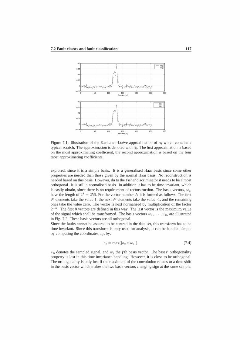
7.2 Fault classes and fault classification 117
0 50 100 150 200 250 300−0.05
0
0.05
0.1
0.15
0.2
Samples [n]
0 50 100 150 200 250 300−0.05
0
0.05
0.1
0.15
0.2
Samples [n]
αfαf
αfαf
Figure 7.1: Illustration of the Karhunen-Loève approximation ofαf which contains atypical scratch. The approximation is denoted withαf . The first approximation is basedon the most approximating coefficient, the second approximation is based on the fourmost approximating coefficients.
explored, since it is a simple basis. It is a generalised Haar basis since some otherproperties are needed than those given by the normal Haar basis. No reconstruction isneeded based on this basis. However, du to the Fisher discriminator it needs to be almostorthogonal. It is still a normalised basis. In addition it has to be time invariant, whichis easily obtain, since there is no requirement of reconstruction. The basis vectors,wi,have the length of28 = 256. For the vector numberN it is formed as follows. The firstN elements take the value 1, the nextN elements take the value -1, and the remainingones take the value zero. The vector is next normalised by multiplication of the factor2−n. The first 8 vectors are defined in this way. The last vector is the maximum valueof the signal which shall be transformed. The basis vectorsw1, · · · , w8, are illustratedin Fig. 7.2. These basis vectors are all orthogonal.Since the faults cannot be assured to be centred in the data set, this transform has to betime invariant. Since this transform is only used for analysis, it can be handled simpleby computing the coordinates,cj , by:
cj = max(|sm ∗ wj |). (7.4)
sm denotes the sampled signal, andwj the j’th basis vector. The bases’ orthogonalityproperty is lost in this time invariance handling. However, it is close to be orthogonal.The orthogonality is only lost if the maximum of the convolution relates to a time shiftin the basis vector which makes the two basis vectors changing sign at the same sample.

118 Time-Frequency Based Feature Extraction of Surface Faults
0 100 200 300−0.5
0
0.5
w1
Samples [n]0 100 200 300
−0.5
0
0.5
w2
Samples [n]
0 100 200 300−0.2
0
0.2
w3
Samples [n]0 100 200 300
−0.1
0
0.1
w4
Samples [n]
0 100 200 300−0.05
0
0.05
w5
Samples [n]0 100 200 300
−0.02
0
0.02
w6
Samples [n]
0 100 200 300−0.01
0
0.01
w7
Samples [n]0 100 200 300
−5
0
5x 10
−3
w8
Samples [n]
Figure 7.2: The 8 generalised Haar basis vectors given the equations in Subsection7.2.2.2.
7.2.2.3 Mean of the classes
Normally a good way to discriminate among signals is to convolute the signal with thesignals them self, and the convolution giving the highest result is the convolution withthe signal itself. But if the signal is not perfectly known or one which is a discriminationof classes containing more than one signal, this method is not so good anymore. How-ever, these arguments indicate the usability of a discriminating basis consisting of themean of the classes. This set is not orthogonal nor does it spanRn, but it is a good setof vectors for the other bases to compare with, since it normally has good discriminatingproperties.
7.2.3 Finding the discriminating basis vectors
The Fisher discriminating power function is following used to find the four most discrim-inating vectors in each basis. These four most discriminating basis vectors are followingused for discrimination.
7.2.3.1 The algorithm
For each class, the centre of the class in the given discriminating basis, is computedbased on the training set. This gives three vectors:C1, C2, C3.The discriminating algorithm is: Find the class which has a centre with the smallest
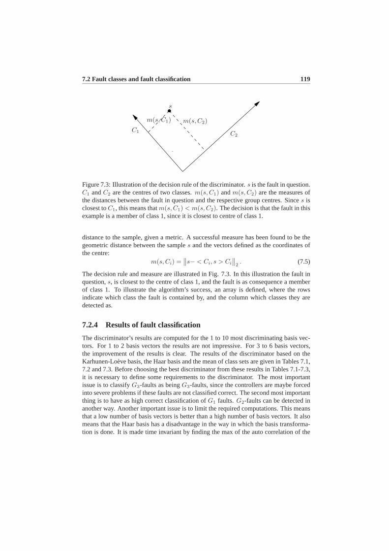
7.2 Fault classes and fault classification 119
s
C1 C2
m(s, C1) m(s, C2)
Figure 7.3: Illustration of the decision rule of the discriminator.s is the fault in question.C1 andC2 are the centres of two classes.m(s, C1) andm(s, C2) are the measures ofthe distances between the fault in question and the respective group centres. Sinces isclosest toC1, this means thatm(s, C1) < m(s, C2). The decision is that the fault in thisexample is a member of class 1, since it is closest to centre of class 1.
distance to the sample, given a metric. A successful measure has been found to be thegeometric distance between the samples and the vectors defined as the coordinates ofthe centre:
m(s, Ci) =∥∥s− < Ci, s > Ci
∥∥2. (7.5)
The decision rule and measure are illustrated in Fig. 7.3. In this illustration the fault inquestion,s, is closest to the centre of class 1, and the fault is as consequence a memberof class 1. To illustrate the algorithm’s success, an array is defined, where the rowsindicate which class the fault is contained by, and the column which classes they aredetected as.
7.2.4 Results of fault classification
The discriminator’s results are computed for the 1 to 10 most discriminating basis vec-tors. For 1 to 2 basis vectors the results are not impressive. For 3 to 6 basis vectors,the improvement of the results is clear. The results of the discriminator based on theKarhunen-Loève basis, the Haar basis and the mean of class sets are given in Tables 7.1,7.2 and 7.3. Before choosing the best discriminator from these results in Tables 7.1-7.3,it is necessary to define some requirements to the discriminator. The most importantissue is to classifyG3-faults as beingG3-faults, since the controllers are maybe forcedinto severe problems if these faults are not classified correct. The second most importantthing is to have as high correct classification ofG1 faults. G2-faults can be detected inanother way. Another important issue is to limit the required computations. This meansthat a low number of basis vectors is better than a high number of basis vectors. It alsomeans that the Haar basis has a disadvantage in the way in which the basis transforma-tion is done. It is made time invariant by finding the max of the auto correlation of the

120 Time-Frequency Based Feature Extraction of Surface Faults
Karhunen-Loève basisαf Karhunen-Loève basisαr
3 Basis vectors 3 Basis vectorsG1 G2 G3
G1 85.7% 25.0% 0.0%G2 9.1% 50.0% 0.0%G3 5.2% 25.0% 100%
G1 G2 G3
G1 83.8% 0.0% 0.0%G2 6.8% 0.0% 16.7%G3 9.5% 100% 83.3%
4 Basis vectors 4 Basis vectorsG1 G2 G3
G1 87.0% 25.0% 0.0%G2 10.4% 50.0% 0.0%G3 2.6% 25.0% 100%
G1 G2 G3
G1 85.1% 0.0% 0.0%G2 8.1% 0.0% 0.0%G3 6.8% 100% 100%
5 Basis vectors 5 Basis vectorsG1 G2 G3
G1 87.0% 25.0% 0.0%G2 10.4% 50.0% 0.0%G3 2.6% 25.0% 100%
G1 G2 G3
G1 83.8% 0.0% 0.0%G2 8.4% 0.0% 16.7%G3 9.5% 100% 83.3%
6 Basis vectors 6 Basis vectorsG1 G2 G3
G1 89.6% 50.0% 0.0%G2 9.1% 25.0% 0.0%G3 1.3% 25.0% 100%
G1 G2 G3
G1 83.8% 0.0% 0.0%G2 2.7% 100% 0.0%G3 13.5% 0.0% 100%
Table 7.1: The results of the discriminator based on the 3 to 6 most discriminatingKarhunen-Loève basis vectors are shown in this table. The left half part of the table isbased on the residualαf [n], and the other half part on the residualαr[n]. These partsare again separated into arrays with the results of each number of basis vectors. ThehorizontalG1, G2, G3 are the class in which the test data are contained and the verticalones are the classes they are classified as being in. This can be illustrated by an example.Takeαf with 3 basis vectors. 85.7%G1-faults were classified as beingG1-faults, 9.1%were classified as beingG2-fault and the remaining 5.2% were classified as beingG3-faults.
basis vectors and the residuals, where the other two basis transformations are done byconvoluting the basis vectors with the residuals. This means that a Haar based approachhas to perform significantly better than the other bases to be chosen, as the best one, andin addition it is time invariant.
Inspection of the three tables with the results show that the best performance is achievedby using the Haar transform with 5 basis vectors onαr[n], whereG1-faults were classi-fied correct with 94.6% success, and the two other classes were correctly classified with100% success. The mean-of-class basis achieves the best performance for theαr[n]residual, with 82.4% success forG1-faults and 100% success for the two others. TheKarhunen-Loève basis performs best at theαf [n] residual. The Karhunen-Loève basisdoes not improve its performance much from 3 to 6 basis vectors. It is interesting tocompare the result of order 3 and 4 discriminator based on the Karhunen-Loève basis,

7.2 Fault classes and fault classification 121
Haar basisαf Haar basisαr
3 Basis vectors 3 Basis vectorsG1 G2 G3
G1 49.4% 50.0% 0.0%G2 19.5% 25.0% 0.0%G3 31.2% 25.0% 100%
G1 G2 G3
G1 75.5% 0.0% 0.0%G2 4.1% 100% 66.7%G3 20.3% 0.0% 33.3%
4 Basis vectors 4 Basis vectorsG1 G2 G3
G1 35.1% 25.0% 0.0%G2 42.9% 50.0% 0.0%G3 22.1% 25.0% 100%
G1 G2 G3
G1 79.7% 0.0% 0.0%G2 16.2% 0.0% 16.7%G3 4.1% 100% 83.3%
5 Basis vectors 5 Basis vectorsG1 G2 G3
G1 54.5% 25.0% 0.0%G2 31.1% 50.0% 0.0%G3 14.3% 25.0% 100%
G1 G2 G3
G1 94.6% 0.0% 0.0%G2 1.4% 100% 0.0%G3 4.1% 0.0% 100%
Basis order 6 Basis order 6G1 G2 G3
G1 84.4% 25.0% 0.0%G2 10.4% 50.0% 0.0%G3 5.2% 25.0% 100%
G1 G2 G3
G1 77.0% 0.0% 0.0%G2 17.6% 100% 0.0%G3 5.4% 0.0% 100%
Table 7.2: The results of the discriminator based on 3 to 6 most discriminating Haar basisvectors are shown in this table. The left half part of the table is based on the residualαf [n], and the other half part on the residualαr[n]. These parts are again separated intoarrays with the results of each number of basis vectors. The horizontalG1, G2, G3
were the class in which the test data were contained and the vertical ones are the classesthey were classified as being in. This is the same principle as in Table 7.1.
Mean setαf Mean setαr
3 vectors 3 vectorsG1 G2 G3
G1 79.2% 0.0% 50.0%G2 13.0% 75.0% 25.0%G3 19.5% 0.0% 25.0%
G1 G2 G3
G1 82.4% 0.0% 0.0%G2 17.6% 100% 0.0%G3 0.0% 0.0% 100%
Table 7.3: The results of the discriminator based on the mean of class set of the order3, this set has only 3 vectors, shown in this table. The left half part of the table isbased on the residualαf [n], and the other half part on the residualαr[n]. The horizontalG1, G2, G3 were the class which the test data were contained in and the vertical oneswere the classes they were classified as being in. This is the same principle as in Table7.1.
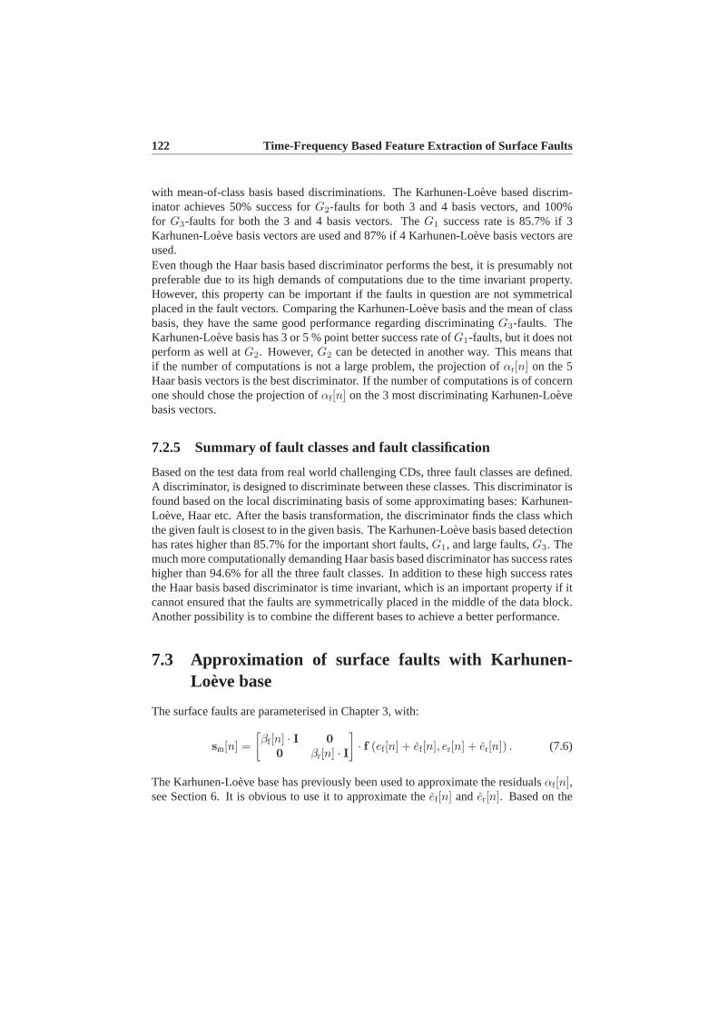
122 Time-Frequency Based Feature Extraction of Surface Faults
with mean-of-class basis based discriminations. The Karhunen-Loève based discrim-inator achieves 50% success forG2-faults for both 3 and 4 basis vectors, and 100%for G3-faults for both the 3 and 4 basis vectors. TheG1 success rate is 85.7% if 3Karhunen-Loève basis vectors are used and 87% if 4 Karhunen-Loève basis vectors areused.Even though the Haar basis based discriminator performs the best, it is presumably notpreferable due to its high demands of computations due to the time invariant property.However, this property can be important if the faults in question are not symmetricalplaced in the fault vectors. Comparing the Karhunen-Loève basis and the mean of classbasis, they have the same good performance regarding discriminatingG3-faults. TheKarhunen-Loève basis has 3 or 5 % point better success rate ofG1-faults, but it does notperform as well atG2. However,G2 can be detected in another way. This means thatif the number of computations is not a large problem, the projection ofαr[n] on the 5Haar basis vectors is the best discriminator. If the number of computations is of concernone should chose the projection ofαf [n] on the 3 most discriminating Karhunen-Loèvebasis vectors.
7.2.5 Summary of fault classes and fault classification
Based on the test data from real world challenging CDs, three fault classes are defined.A discriminator, is designed to discriminate between these classes. This discriminator isfound based on the local discriminating basis of some approximating bases: Karhunen-Loève, Haar etc. After the basis transformation, the discriminator finds the class whichthe given fault is closest to in the given basis. The Karhunen-Loève basis based detectionhas rates higher than 85.7% for the important short faults,G1, and large faults,G3. Themuch more computationally demanding Haar basis based discriminator has success rateshigher than 94.6% for all the three fault classes. In addition to these high success ratesthe Haar basis based discriminator is time invariant, which is an important property if itcannot ensured that the faults are symmetrically placed in the middle of the data block.Another possibility is to combine the different bases to achieve a better performance.
7.3 Approximation of surface faults with Karhunen-Loève base
The surface faults are parameterised in Chapter 3, with:
sm[n] =[βf [n] · I 0
0 βr[n] · I]· f (ef [n] + ef [n], er[n] + er[n]) . (7.6)
The Karhunen-Loève base has previously been used to approximate the residualsαf [n],see Section 6. It is obvious to use it to approximate theef [n] and er[n]. Based on the
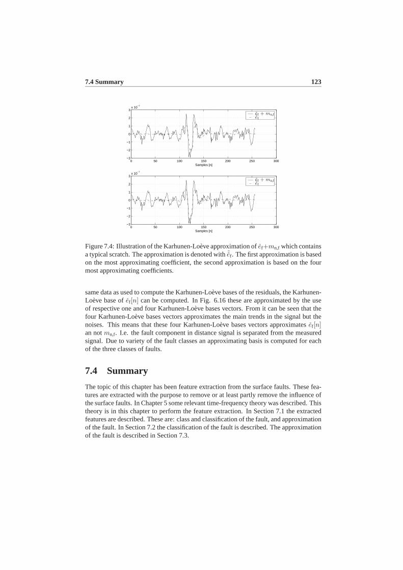
7.4 Summary 123
0 50 100 150 200 250 300−3
−2
−1
0
1
2
3x 10
−7
Samples [n]
0 50 100 150 200 250 300−3
−2
−1
0
1
2
3x 10
−7
Samples [n]
ef + mn,f˜ef
ef + mn,f˜ef
Figure 7.4: Illustration of the Karhunen-Loève approximation ofef+mn,f which containsa typical scratch. The approximation is denoted with˜ef . The first approximation is basedon the most approximating coefficient, the second approximation is based on the fourmost approximating coefficients.
same data as used to compute the Karhunen-Loève bases of the residuals, the Karhunen-Loève base ofef [n] can be computed. In Fig. 6.16 these are approximated by the useof respective one and four Karhunen-Loève bases vectors. From it can be seen that thefour Karhunen-Loève bases vectors approximates the main trends in the signal but thenoises. This means that these four Karhunen-Loève bases vectors approximatesef [n]an notmn,f. I.e. the fault component in distance signal is separated from the measuredsignal. Due to variety of the fault classes an approximating basis is computed for eachof the three classes of faults.
7.4 Summary
The topic of this chapter has been feature extraction from the surface faults. These fea-tures are extracted with the purpose to remove or at least partly remove the influence ofthe surface faults. In Chapter 5 some relevant time-frequency theory was described. Thistheory is in this chapter to perform the feature extraction. In Section 7.1 the extractedfeatures are described. These are: class and classification of the fault, and approximationof the fault. In Section 7.2 the classification of the fault is described. The approximationof the fault is described in Section 7.3.


Chapter 8
A Simulation Model
Previous designs of fault tolerant controllers of CD-players have been based on trial anderror on real test systems since no simulation models including the surface faults havebeen available. The CD-player servos consist roughly of two parts: an electro-magnetic-mechanical part - the actuator, and the electro-optical part - the sensor. Another impor-tant part of the system is the surface faults on the CDs, if one would like to handle those.These parts are modelled in Chapter 3.
In [Odgaard and Wickerhauser, 2003] some work is done on finding a good approxi-mating basis of the surface faults. It is done by finding the Karhunen-Loève basis, seeChapters 5 and 6, on a set of experimental data with faults.
By using a Karhunen-Loève basis, based on the experimental data, the faults can beapproximated with a few coefficients. This can be used to simulate faults, by computingthe required coefficients by random numbers with the same mean and variance as thetraining data did have.
In this chapter the model of the CD-player and surface faults are summarised, see Sec-tion 8.1. The simulation model is developed based on a Karhunen-Loève approximationof surface faults, and the mean and variance of the experimental data. In addition dis-turbances and measurement noises are added at the relevant places in the system, seeSection 8.2. This chapter does not deal with fault tolerant control, but with a simulationmodel of CD-player. This model simulates both the focus and radial loop, this meansthat simulations require both a focus and a radial controller. In order to show this modelin practice two simulations are performed in closed loop with two different pairs of PID-controllers with and without a surface fault. The first simulated pair of controllers havea high bandwidth which makes it good for handling disturbances. The second simulatedpair of controllers have a lower bandwidth which makes it better suited for handlingsurface faults, see Section 8.3.
125

126 A Simulation Model
8.1 Model
The idea of the discrete time model is to simulate focus and radial servo loops in CD-players with relevant disturbances as well as surface faults represented by models basedon experimental data. This model of the focus and radial servos in the CD-player isderived in Chapter 3. The simulation model includes some extra parts compared with themodel derived in Chapter 3. The overall structure of this simulation model is illustratedin Fig. 8.1. The controllers’ jobs are to keep the OPU focused and radially tracked on thedisc information track. The actuator used to move the OPU in focus and radial directionsis a 2-axis linear electro magnetic actuator. This Electro Mechanical System (EMS) is
used to set the OPUs absolute position,x[n] =[xf [n]xr[n]
]. The track position is given by
the position referencexref[n] =[xref,f[n]xref,r[n]
]. These references are due to eccentricity and
skewness of the disc, since these dominates the inherited reference given by the spiralshaped track. I.e. the vector of distance signals can be defined as:e[n] = xref[n]−x[n].The Optical System, OS, is used to retrieve data from the disc and to generate four
detector signals,s[n] =[D1[n], D2[n], S1[n], S2[n]
]T, which are used to approximate
the focus and radial errors. This approximation is done in the Signal Converter, SC. TheSC computes normalised approximations of the error signals,en[n]. In Chapter 3, theentire CD-player model is derived as follows
sm[n] =[βf [n] · I2×2 0
0 βr[n] · I2×2
]· f (ef [n] + ef [n], er[n] + er[n]) , (8.1)
wheref (·) is the model of the optical detectors, see (3.13)-(3.51). Focus and radialdistancesef [n] ander[n] are modelled in (3.11) and (3.12).βf [n], βr[n] are two faultmodel parameters. This fault model can be explained, but unfortunately a fault affectsthe detector signal in another more problematic way. Surface faults also introduce faultyfocus and radial errors,e[n], which are added toe[n]. The task of the controller is to keepthe OPU focused and radially tracked. It is done by feeding the EMS with control signalsu[n] calculated from past and present values ofen[n]. In order to simulate externaldisturbances like shocks and internal not model selfpollutions, a vector of disturbancesignals,d[n] is added tou[n] before they are fed to the EMS.
8.2 Surface fault synthesiser
The surface faults are parameterised in (8.1). The next step is to synthesise the valuesof these parameters during a fault. One approach would be to take measured data froma real CD-player playing a CD with a surface fault and use these measured data in thesimulation representing a surface fault. This approach has a severe drawback, it limitsthe number of possible faults in simulation to those measured. In this chapter another
8.2 Surface fault synthesiser 127
OS
DS
SC
−Controller EMS ++ +u
dexxref
s sm
Be
en
Figure 8.1: Illustration of the structure of the CD-player simulations model. The sub-models in the models are as follows. EMS, denotes the Electro Mechanical system,OS is the Optical System of the OPU. DS denotes the Fault Synthesiser, and simulatessurface faults. SC denotes the Signal Converter which computes normalised focus andradial differences which are approximations of focus and radial distances. In additionfocus and radial disturbance,d[n], and an unknown references,eref[n], are added to thesystem.
approach is presented, which is based on Karhunen- Loève approximations of the faults,see Chapter 6.Blocks of 256 samples are extracted from experimental data, where each block containsat least one fault. The experimental data represent fingerprints, short and long scratchesetc. In Section 3.1 the experimental setup used to measure the data is described. Byinspection the experimental data are separated into three classes in Section 7.2: shortand long scratches and disturbance like faults.The next step in this approach is to compute the best approximating basis of this dataset - the Karhunen-Loève basis, see Chapter 5 and [Mallat, 1999]. The approximatingpotentials are illustrated in Fig. 7.2. This illustrates a scratch approximated with themost approximating coefficient and the four most approximating coeffiecients respec-tively. Note the approximation with only one coefficient is a good approximation of thescratch.Denote a matrix, where the column vectors are vectors of zero mean data,S. TheKarhunen-Loève basis, see Section 5.5,K, of S is the set of eigenvectors of the au-tocorrelation ofS:
K = {eigenvectors(SST
)}. (8.2)
The Karhunen-Loève basis of all the measuredβf [n] is denotedKβf . Kβr denotes theKarhunen-Loève basis of measuredβr[n]. Kef , Ker denote the Karhunen-Loève basisof ef [n] and er[n] computed based on measurements, which also contain measurementnoises etc.Assume that each of the measured faults consists of a signal part and a noise part. Usingthe Karhunen-Loève basis the signal part can be approximated with a few coordinates

128 A Simulation Model
in that basis, (the firstk coefficients). The remaining noise part could be approximatedwith the remaining,N − k coefficients. Next compute the meanmi and varianceσi
of each coordinate. Assume that each Karhunen-Loève coordinate can be simulated asindependently distributed normal random variables withσi andmi, where these statis-tics are found based on the Karhunen-Loève coordinates. The signal part can then besynthesised as:
Ssyn =k∑
i=1
Ksyn,ick,i, (8.3)
and the noise as
Ssyn,N =N∑
i=k+1
Ksyn,ick,i, (8.4)
where
Ksyn ∈ {Kβf ,Kβr ,Kef ,Ker}, (8.5)
ck,i ∈ Ni(mi, σi), (8.6)
andSsyn denote the synthesisedβf , βr, ef , er, andSsyn,N the noise part of these. Sincek ¿ n the signal synthesis is cheap in computations, but the noise part is expensive.Instead the noise signal can be computed as
Ssyn,N =
y1
...yi
...yN
(8.7)
, whereyi ∈ N (0, σ√N
) is independent,σ is equal√
σ2k+1 . . . σ2
N . The coordinates
in the noise vector are independent, identically distributed normal random variables,since the following is well known, If T:RN → RN is orthonormal andy is defined in(8.7), then the coordinates ofTy are independent, identically distributed normal randomvariables signal with same mean, 0, and variance,σ√
N.
It is now possible to synthesise a fault. The statistics used for the fault constructionis based on all faults in a fault class. However, a fault does not vary much from oneencounter to the next encounter, see Section 6.1. This fact has to be taking into accountwhen the next fault encounter is simulated, see Section 5.σi is computed as the mean ofthe variances of coefficients of sequently following encounters of faults. The mean usedin the construction is the simulated coefficient value from the last fault encounter.

8.2 Surface fault synthesiser 129
This fault synthesiser constructs the faults in blocks of 256 meaning that it is requiredto compute a long block of fault parameters before the simulation of the CD-player, andthen during the simulation use these computed values.
8.2.1 Disturbances and references
The CD-player’s unknown reference is mainly due to eccentricity and skewness. Itis computed as a sine with the period being the rotation period of the given rotation.These periods increase with one sample each third rotation, due to the linearly increasedrotation length measured in number of samples, due to the spiral shaped informationtrack on the disc. The amplitude of the reference can freely be chosen, (with the playerrequirements stated in [Stan, 1998]), and in this simulation both are chosen to be 30µm.The disturbances are white noise added to the control signals, where the variance 0.01is chosen based on experience.
40
45
50
55
60
65
70
75
80
Mag
nitu
de (
dB)
101
102
103
104
105
−180
−90
0
90
Pha
se (
deg)
Bode Diagram
Frequency (rad/sec)
Figure 8.2: Bode plot of the nominal focus controller.
8.2.2 Signal converter
The Signal Converter is described in Section 3.5, where it is described that focus andradial distances are approximated by the use of the normalised difference betweenD1
andD2 for focus andS1 andS2 for radial. This means
en =
[D1−D2D1+D2S1−S2S1+S2
](8.8)
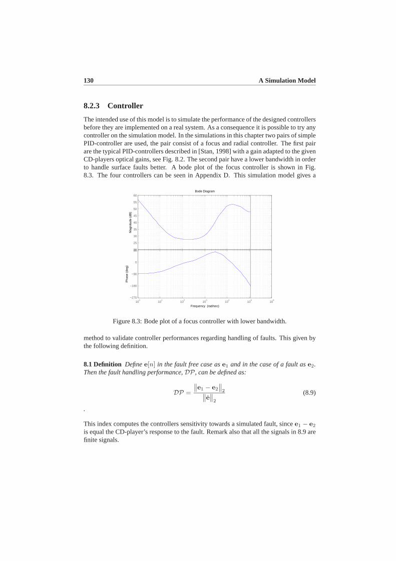
130 A Simulation Model
8.2.3 Controller
The intended use of this model is to simulate the performance of the designed controllersbefore they are implemented on a real system. As a consequence it is possible to try anycontroller on the simulation model. In the simulations in this chapter two pairs of simplePID-controller are used, the pair consist of a focus and radial controller. The first pairare the typical PID-controllers described in [Stan, 1998] with a gain adapted to the givenCD-players optical gains, see Fig. 8.2. The second pair have a lower bandwidth in orderto handle surface faults better. A bode plot of the focus controller is shown in Fig.8.3. The four controllers can be seen in Appendix D. This simulation model gives a
20
25
30
35
40
45
50
55
60
Mag
nitu
de (
dB)
100
101
102
103
104
105
106
−270
−180
−90
0
90
Pha
se (
deg)
Bode Diagram
Frequency (rad/sec)
Figure 8.3: Bode plot of a focus controller with lower bandwidth.
method to validate controller performances regarding handling of faults. This given bythe following definition.
8.1 Definition Definee[n] in the fault free case ase1 and in the case of a fault ase2.Then the fault handling performance,DP, can be defined as:
DP =
∥∥e1 − e2
∥∥2∥∥e∥∥
2
(8.9)
.
This index computes the controllers sensitivity towards a simulated fault, sincee1 − e2
is equal the CD-player’s response to the fault. Remark also that all the signals in 8.9 arefinite signals.

8.3 Simulations of a CD-player playing a CD with surface faults 131
8.3 Simulations of a CD-player playing a CD with sur-face faults
The simulations are performed in closed loop, where the two simulated controllers con-trol the CD-player model, with the objective to suppress the disturbances and the un-known reference. The first simulations of the two controllers are simulations withoutany surface faults. These fault free simulation are important in order to validate thegiven controllers capability to handle a fault, since any differences from these are dueto the fault, and not the controllers ability to suppress disturbances. These signals are asconsequence used in Def. 8.1 where these errors are denotede1.The controllers react to a sum of the real distances and the faulty distance components.To illustrate how the controller forces the system out of focus and radial tracking duringa fault, the simulated real distances are illustrated and not the distances used for con-trolling the system, since they contain the faulty component too. The simulation outputof the normal PID-controller can be seen in Fig. 8.4 which is a zoom on a fault. Thesecond subfigure in Fig. 8.4, is a zoom on the fault,ef [n]. This means that the controllerreacts on the focus error component due to the fault,ef [n], which is undesired. The con-troller with a lower bandwidth is illustrated as well in Fig. 8.4. This figure shows thatthe low bandwidth controller handles the fault better than the normal one. The upperplot in Fig. 8.4 do also validate the simulation model, since this close loop output ofthe nominal controller, is similar to the measured focus distance during a surface faultwhere the focus distance is controlled by the nominal controller.The two controllers can be compared by using Def. 8.1. The computed indexes can beseen in Table 8.1, in addition the nominal performances,NP, are also computed definedas:
NP =rms(e1)
rms(xref) + rms(d)(8.10)
The two-norm of the error signal can be use to compare the nominal performance of thetwo controllers since the same reference, disturbances and faults are applied to them inthe simulations. The performance index consists of two elements the first is the focusindex and the second element is the radial index. Based on these results it can be seenthat the nominal controller is better for handling disturbances, but on the other hand thelow bandwidth PID-controller is better for handling the surface faults. This supports theknown controller specification conflict between handling faults and disturbances. Oneshould notice that the simulated fault in this situation is a small fault, which controllersnormally survives, but in a non-optimal way. Handling larger faults cause larger prob-lems for the controller, meaning that a fault tolerant approach is relevant in order not toreact to surface faults, where surface faults are viewed as being sensor faults. The use ofthis simulation model has a potential to make the design of controllers handling surfacefault faster, since the use of simulations can eliminate some of the practical experimentsin the controller design process.The simulations are implemented in MATLAB . The used MATLAB script files and
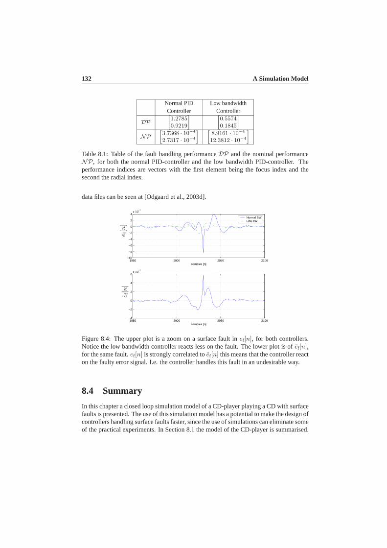
132 A Simulation Model
Normal PID Low bandwidthController Controller
DP»1.27850.9219
– »0.55740.1845
–
NP»3.7368 · 10−4
2.7317 · 10−4
– »8.9161 · 10−4
12.3812 · 10−4
–
Table 8.1: Table of the fault handling performanceDP and the nominal performanceNP, for both the normal PID-controller and the low bandwidth PID-controller. Theperformance indices are vectors with the first element being the focus index and thesecond the radial index.
data files can be seen at [Odgaard et al., 2003d].
1950 2000 2050 2100−10
−8
−6
−4
−2
0
2
4x 10
−7
samples [n]
1950 2000 2050 2100−4
−2
0
2
4
6x 10
−7
samples [n]
Normal BWLow BW
e f[n
]e f
[n]
Figure 8.4: The upper plot is a zoom on a surface fault inef [n], for both controllers.Notice the low bandwidth controller reacts less on the fault. The lower plot is ofef [n],for the same fault.ef [n] is strongly correlated toef [n] this means that the controller reacton the faulty error signal. I.e. the controller handles this fault in an undesirable way.
8.4 Summary
In this chapter a closed loop simulation model of a CD-player playing a CD with surfacefaults is presented. The use of this simulation model has a potential to make the design ofcontrollers handling surface faults faster, since the use of simulations can eliminate someof the practical experiments. In Section 8.1 the model of the CD-player is summarised.

8.4 Summary 133
In Section 8.2 a surface fault synthesiser is derived. The simulations show that thefocus and radial servo, in a typical CD-player, react on the fault in a non-desired way.In addition a controller with a lower bandwidth is simulated. A performance index ofthe controllers handling fault is also defined and used to compare the two simulatedcontrollers. This comparison validates a known fact that handling disturbances in CD-players requires a high bandwidth and handling surface faults on CDs requires a lowbandwidth, see Section 8.3.


Chapter 9
Feature Based Control ofCompact Disc Players
In this chapter the core of this feature based control scheme of the CD-player will bedescribed and designed. This algorithm is based on the work presented in the previ-ous chapters. The idea in short is, that the residuals computed in Chapter 4 are usedto detect and locate the surface faults, by the use of the algorithms presented in Chap-ter 6. The feature extraction presented in Chapter 7 gives a classification of the faultas well as approximating coefficients in a given basis representing the class of thefault. The feature based control algorithm is presented in the following sections andin [Odgaard et al., 2004c] and [Odgaard et al., 2004b]. In Section 9.1 the feature basedcontrol scheme is introduced and described in general terms and related to the fault toler-ant control method. This leads to fault accommodation part of the feature based controlalgorithm which is described in Section 9.2. Some stability and performance issues arediscussed in Section 9.3, where it is proven that the method is stable. In Section 9.4the simulation model derived in Chapter 8 is used to simulate the feature based controlscheme handling a CD with a scratch. These simulations are followed by experimentalresults presented in Section 9.5.
9.1 Feature based control versus fault tolerant control
An overview of the feature based control scheme was presented in Section 2.9. Thefeature based control strategy is illustrated in Fig. 2.12, from which it can be seen thatthe feature based control strategy consists of: residual and distance estimation, fault de-tector/fault locator, feature extraction, fault accommodation. The residual and distanceestimation estimates the decoupled residuals and focus and radial distances. The faultdetector/locator detects and locates the fault in time. The time localisation gives infor-
135

136 Feature Based Control of Compact Disc Players
mation of when to extract features and when to accommodate the fault. The featureextraction feeds the fault accommodation with the class of the fault and approximatingcoefficients in an approximating basis of the given class of the fault. This feature basedcontrol strategy is strongly related to fault tolerant control scheme. In order to explainthis relation, the fault tolerant control method is presented.
Fault tolerant control Two types of fault tolerant controllers can be designed. Theactive fault tolerant control, where the fault is accommodated when the fault is detected,and passive fault tolerant control, where the controllers are designed to stabilise theclosed loop system in case of a fault. In this work only the active fault tolerant controlis considered. Fault tolerant control methods normally consist of two parts which are:
• Fault detection and isolation (FDI): detects, isolates and estimates the fault.
• Fault accommodation: based on the detection, isolation and estimation of thefault, is the fault accommodated.
More information on fault accommodation and fault tolerant control is given in[Blanke et al., 2003].Some examples of descriptions on fault detection and isolation are [Patton et al., 1989],[Gertler, 1998], [Frank, 1990] and [Chen and Patton, 1991]. The purpose of fault diag-nosis is to diagnose the fault as early as possible before it develops and leads to severeconsequences. In order to avoid these, this fault diagnosis consists of three parts: faultdetection, fault isolation and fault estimation. In the normal usage the fault detectionand fault isolation are essential in the fault diagnosis, these are often denoted FDI, onthe other hand the fault estimation is not strictly necessary. However, in this applica-tion the fault detection and fault estimation are essential, and the fault isolation is notimportant, since the fault detection is used to detect a given kind of fault.This leads to a fault detection and isolation (FDI) scheme consisting of the followingthree steps:
• Fault detection: is to detect the occurrence of a fault, typically indicated with a bitindicating the occurrence of a fault or not.
• Fault isolation: is to determine the origin of the fault.
• Fault estimation: is estimation of size and type of the fault, and of the fault itself.
Feature based control and fault tolerant control The fault detection/locator per-forms the fault detection, by locating the fault in time. The fault isolation in this situationis different from the standard fault isolation. Normally fault isolation is used to isolatethe fault to be in a specific place in the system. In this application only surface faults areconsidered. By the construction of the decoupled residuals, the fault is isolated to be asurface fault. The estimation of the fault is performed by fault classification and approx-imation of the fault, where a disturbance decoupled fault estimation is performed. This
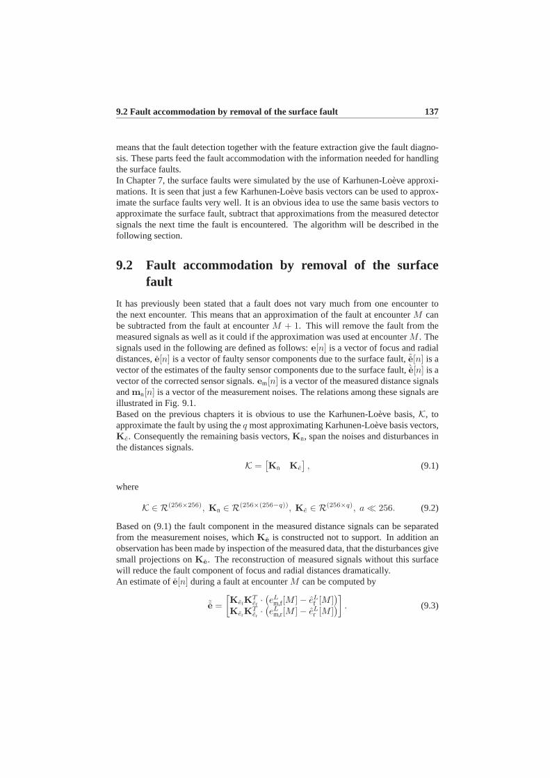
9.2 Fault accommodation by removal of the surface fault 137
means that the fault detection together with the feature extraction give the fault diagno-sis. These parts feed the fault accommodation with the information needed for handlingthe surface faults.In Chapter 7, the surface faults were simulated by the use of Karhunen-Loève approxi-mations. It is seen that just a few Karhunen-Loève basis vectors can be used to approx-imate the surface faults very well. It is an obvious idea to use the same basis vectors toapproximate the surface fault, subtract that approximations from the measured detectorsignals the next time the fault is encountered. The algorithm will be described in thefollowing section.
9.2 Fault accommodation by removal of the surfacefault
It has previously been stated that a fault does not vary much from one encounter tothe next encounter. This means that an approximation of the fault at encounterM canbe subtracted from the fault at encounterM + 1. This will remove the fault from themeasured signals as well as it could if the approximation was used at encounterM . Thesignals used in the following are defined as follows:e[n] is a vector of focus and radialdistances,e[n] is a vector of faulty sensor components due to the surface fault,˜e[n] is avector of the estimates of the faulty sensor components due to the surface fault,`e[n] is avector of the corrected sensor signals.em[n] is a vector of the measured distance signalsandmn[n] is a vector of the measurement noises. The relations among these signals areillustrated in Fig. 9.1.Based on the previous chapters it is obvious to use the Karhunen-Loève basis,K, toapproximate the fault by using theq most approximating Karhunen-Loève basis vectors,Ke. Consequently the remaining basis vectors,Kn, span the noises and disturbances inthe distances signals.
K =[Kn Ke
], (9.1)
where
K ∈ R(256×256), Kn ∈ R(256×(256−q)), Ke ∈ R(256×q), a ¿ 256. (9.2)
Based on (9.1) the fault component in the measured distance signals can be separatedfrom the measurement noises, whichKe is constructed not to support. In addition anobservation has been made by inspection of the measured data, that the disturbances givesmall projections onKe. The reconstruction of measured signals without this surfacewill reduce the fault component of focus and radial distances dramatically.An estimate ofe[n] during a fault at encounterM can be computed by
˜e =[KefK
Tef· (eL
m,f[M ] − eLf [M ]
)KerK
Ter· (eL
m,r[M ] − eLr [M ]
)] . (9.3)
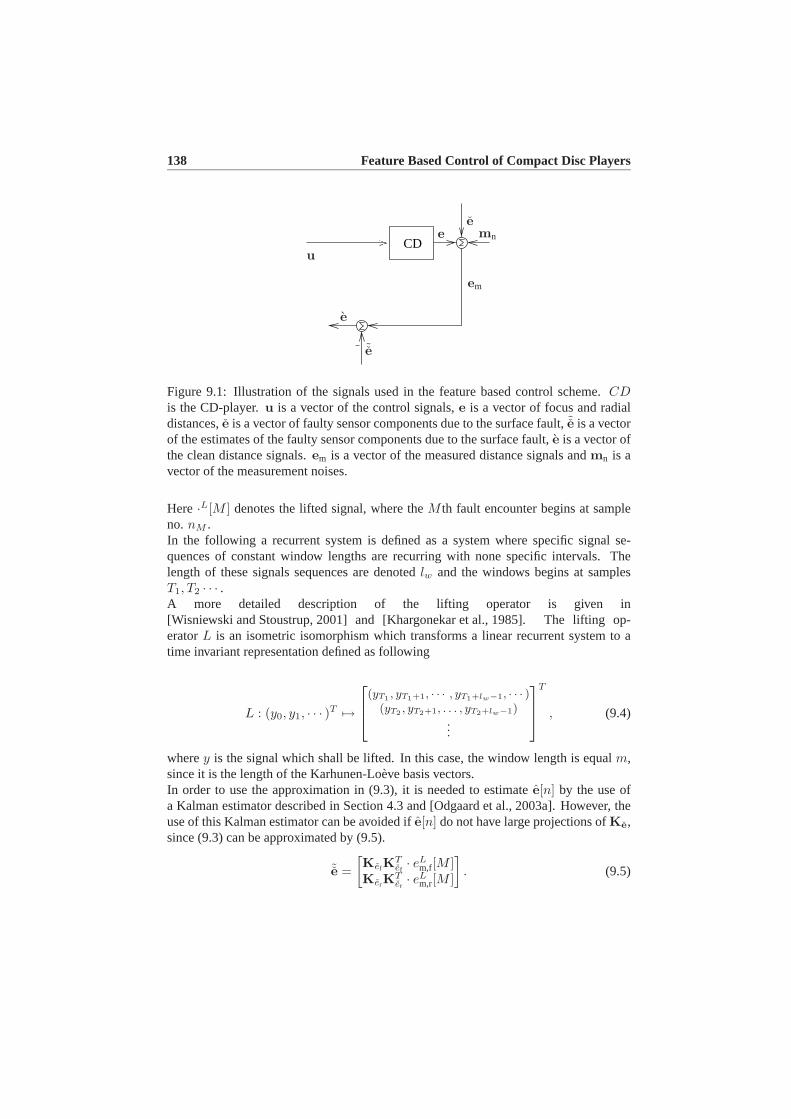
138 Feature Based Control of Compact Disc Players
CDu
ee
e
˜e
em
mn
Figure 9.1: Illustration of the signals used in the feature based control scheme.CDis the CD-player.u is a vector of the control signals,e is a vector of focus and radialdistances,e is a vector of faulty sensor components due to the surface fault,˜e is a vectorof the estimates of the faulty sensor components due to the surface fault,e is a vector ofthe clean distance signals.em is a vector of the measured distance signals andmn is avector of the measurement noises.
Here ·L[M ] denotes the lifted signal, where theM th fault encounter begins at sampleno. nM .In the following a recurrent system is defined as a system where specific signal se-quences of constant window lengths are recurring with none specific intervals. Thelength of these signals sequences are denotedlw and the windows begins at samplesT1, T2 · · · .A more detailed description of the lifting operator is given in[Wisniewski and Stoustrup, 2001] and [Khargonekar et al., 1985]. The lifting op-eratorL is an isometric isomorphism which transforms a linear recurrent system to atime invariant representation defined as following
L : (y0, y1, · · · )T 7→
(yT1 , yT1+1, · · · , yT1+lw−1, · · · )(yT2 , yT2+1, . . . , yT2+lw−1)
...
T
, (9.4)
wherey is the signal which shall be lifted. In this case, the window length is equalm,since it is the length of the Karhunen-Loève basis vectors.In order to use the approximation in (9.3), it is needed to estimatee[n] by the use ofa Kalman estimator described in Section 4.3 and [Odgaard et al., 2003a]. However, theuse of this Kalman estimator can be avoided ife[n] do not have large projections ofKe,since (9.3) can be approximated by (9.5).
˜e =[KefK
Tef· eL
m,f[M ]KerK
Ter· eL
m,r[M ]
]. (9.5)
9.2 Fault accommodation by removal of the surface fault 139
The Kalman estimator is only used to estimatee[n], this means that a consequence of(9.5) is that the Kalman estimator is not needed in the closed loop feature based controlscheme, but it is needed in order to compute the Karhunen-Loève basis of the surfacefaults. This means that if focus and radial distances are in the nominal operation range,the faults can be approximated by the use of the normalised focus and radial differencesignals:
em,f[n] ≈ kf · D1[n] − D2[n]D1[n] + D2[n]
, (9.6)
em,r[n] ≈ kr · S1[n] − S2[n]S1[n] + S2[n]
, (9.7)
wherekf is the optical gain in the focus loop andkr is the optical gain in the radial loop.Due to limitations in the PC computational powers only the approach with out theKalman estimator is tested on the test setup. An extension of the proposed methodcould contain an adaptive scheme where the basis is trained based on faults on a givenCD.The stability and performance issues of the removal is dealt with in Section 9.3.The approximation of the surface fault is now computed. The next problem is to deter-mine when to begin the correction of focus and radial distances. This involves a syn-chronisation of the correction with the distance signals, where a correct synchronisationresults in a removal of the fault from the measurements. An incorrect synchronisationmight result in an increase of the controller reaction to the surface fault, and could ac-tually make the problem with the surface faults more severe than if no correction wasperformed.
9.2.1 Synchronisation of the fault removal
In order to synchronise the correction of the measured signals two methods were used:detection of beginning and end of the surface fault, and prediction of the next fault basedon previous encounters of the faults. The first method uses detection at a given fault tocorrect this given fault. This method has a good synchronisation, but unfortunately hasthe drawback that it locates the beginning and end of the faults respectively too late andtoo early. Using the previous location of the fault in time to predict the next fault, makesit possible to begin and end the correction at a more correct time than if detection basedon the given fault is used. This prediction is based on some time localisation schemee.g. the ones developed in Chapter 6 and [Odgaard and Wickerhauser, 2004]. However,it is not possible in practical settings to predict the placement of a fault. The reason forthis is the implementation of the controller of the disc motor, which should guaranteea constant linear speed of the OPU relative to the track. However, this controller isimplemented in a way that does not result in a constant linear speed but only in a linearspeed in intervals.

140 Feature Based Control of Compact Disc Players
Prediction interval
Fault location
Figure 9.2: Illustration on the fault location and the interval in which the fault is located.
RemovalFault
Normal
ApproxFault
UpdateFault
fd = 0
fd = 1
fd = 0
fd = 1fd = 1
fu = 1
fu = 1
Figure 9.3: Illustration of the feature based control scheme illustrated as a state ma-chine. The dashed lines do not illustrate state changes but data transfers.fd denotes thedetection signal, if a fault is detected at samplen it has 1 as its value, if a fault is notpresent it takes the value 0.fu denotes an indication of the fault has been updated. TheFault Removal represents step 2 in the feature based control scheme and Fault Updaterepresents step 3-5 in this scheme.
In practice a combination of the two fault localisation methods are used. The prediction,based on the time localisation methods presented in [Odgaard and Wickerhauser, 2004],is used to give an interval in which the fault is located and in this interval a lower thres-hold, than if the prediction was not used, can be used, see Fig. 9.2.
9.2.2 The algorithm of the feature based control strategy
The fault correction algorithm can now be stated:
1. Detect the fault and locate its position in time, when the fault is detected at samplen, fd[n] = 1.
9.2 Fault accommodation by removal of the surface fault 141
2. If fd[n] = 1:
a =
{0 if fd[n − 1] = 0,a + 1 if fd[n − 1] = 1.
,
e[n] = em[n] −[˜ef [ι]˜er[ι]
],
where
ι = ((256 − lf) div (2)) + a,
wherea is a counter counting the number of samples the given fault is present,andι is a counter used to locate the given sample relative to the fault correctionblock.
3. When the fault has been passed, classify the fault, time locate the fault, and com-pute the fault lengthlf .
4. Compute the focus correction block coefficients by:kf = Kef · em,f[υ] and theradial correction coefficients by :kr = Ker · em,r[υ], whereυ is the interval of 256samples in which the fault is present.
5. Compute the focus fault removal correction block by:˜ef = Kef ·kf , and the radialfault removal correction by:er = Ker · kr.
In the following,P(·) denotes an operator that maps measured signals into “repaired”ones by applying the correction algorithm. Due to the design ofKe it does in principlenot make any difference ifem[n] or em[n] − e[n] is used to estimate the surface fault,sinceKe is designed to supporte[n] and assumed not supportem[n]. This means that
P (em[n]) ≈ P (e) [n] ⇒ (9.8)
P (e) [n] ≈ 0. (9.9)
Which in turn implies that it is not necessary to estimatee[n]. The normed focus andradial differences, (9.6, 9.7), can be used instead and thereby saves computing power.Only the last one is implemented due to limitations in the computer power in the exper-imental setup.
9.2.3 Practical implementation of the algorithm
The implementation uses only the four most approximating basis vectors, of a givenfault class for each of two distance signals. The four basis vectors are chosen in order tolimit the number of computations in the algorithm, and since experiments have shownthat these four basis vectors approximate the faults very well see above. In order to avoid
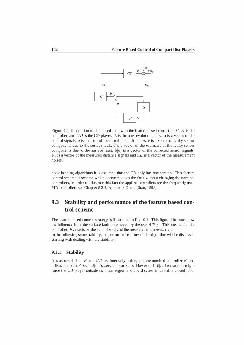
142 Feature Based Control of Compact Disc Players
CD
u
ee
e
˜e
em
mn
K
P
∆
Figure 9.4: Illustration of the closed loop with the feature based correctionP, K is thecontroller, andCD is the CD-player.∆ is the one revolution delay.u is a vector of thecontrol signals,e is a vector of focus and radial distances,e is a vector of faulty sensorcomponents due to the surface fault,˜e is a vector of the estimates of the faulty sensorcomponents due to the surface fault,`e[n] is a vector of the corrected sensor signals.em is a vector of the measured distance signals andmn is a vector of the measurementnoises.
book keeping algorithms it is assumed that the CD only has one scratch. This featurecontrol scheme is scheme which accommodates the fault without changing the nominalcontrollers, in order to illustrate this fact the applied controllers are the frequently usedPID-controllers see Chapter 8.2.3, Appendix D and [Stan, 1998].
9.3 Stability and performance of the feature based con-trol scheme
The feature based control strategy is illustrated in Fig. 9.4. This figure illustrates howthe influence from the surface fault is removed by the use ofP(·). This means that thecontroller,K, reacts on the sum ofe[n] and the measurement noises,mn.In the following some stability and performance issues of the algorithm will be discussedstarting with dealing with the stability.
9.3.1 Stability
It is assumed that:K andCD are internally stable, and the nominal controllerK sta-bilises the plantCD, if e[n] is zero or near zero. However, ife[n] increases it mightforce the CD-player outside its linear region and could cause an unstable closed loop.

9.3 Stability and performance of the feature based control scheme 143
On the other hand ife[n] ≈ e[n] the effect from the surface fault has been removed fromthe closed loop. This means that the control signal would be same as in the fault freecase, meaning that the system is stable since it is nominally stable.P reconstruct therecurrent part of the measurement signals meaning that
em − P (em) ≈= e + mn. (9.10)
This can be achieved if
e ≈ P (em) ⇒ (9.11)
P (mn) ≈ 0 ∧ P (e) ≈ 0 ∧ (9.12)
e = P (e) . (9.13)
This is fulfilled if the approximating bases inP (·) does approximatee[n] well and note[n], mn[n]. P (·) is designed to be the best approximating basis ofe[n]. The Karhunen-Loève basis is not designed to supporte[n], but no guarantees are given that it does notsupporte[n]. InsteadP (·) might amplify the system dynamic in a degree that causesthe entire system to be non-stable. From this it is clear thatP (·)’s amplification ofthe system dynamic shall be small, such that the energy in a given system response isdecreased throughP (·) from revolution to revolution. By inspecting Fig. 9.4 it can beseen that the way the feature based control scheme influences the control loop, such thatinfluence can be analysed by using the complementary sensitivity of the servo system.The influence from the feature based fault handling on the nominal servo system can beinspected if theT denotes the complementary sensitivity of the nominal servo system,and∆ is the one revolution delay, see Fig. 9.5.In order to combine these part systems, the complementary sensitivity of the nominalservo system andP are lifted, meaning that both part systems are represented by adiscrete time series of a given length.The liftedP can be computed by
PL = Ke · KTe , (9.14)
and the lifted representation of the complementary sensitivity is
T L =
h0 0 · · · 0
h1 h0
......
. ..h255 · · · h0
, (9.15)
whereh =[h0 h1 · · · h255
]is time series of 256 samples of the impulse response
of T .
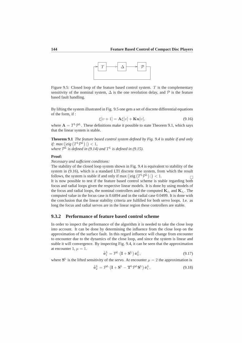
144 Feature Based Control of Compact Disc Players
T ∆ P
Figure 9.5: Closed loop of the feature based control system.T is the complementarysensitivity of the nominal system,∆ is the one revolution delay, andP is the featurebased fault handling.
By lifting the system illustrated in Fig. 9.5 one gets a set of discrete differential equationsof the form, if :
ξ[υ + 1] = Aξ[υ] + Ku[υ], (9.16)
whereA = T LPL. These definitions make it possible to state Theorem 9.1, which saysthat the linear system is stable.
Theorem 9.1 The feature based control system defined by Fig. 9.4 is stable if and onlyif: max
(|eig(T LPL
) |) < 1,wherePL is defined in (9.14) andT L is defined in (9.15).
Proof:Necessary and sufficient conditions:The stability of the closed loop system shown in Fig. 9.4 is equivalent to stability of thesystem in (9.16), which is a standard LTI discrete time system, from which the resultfollows, the system is stable if and only if max
(|eig(T LPL
) |) < 1.It is now possible to test if the feature based control scheme is stable regarding bothfocus and radial loops given the respective linear models. It is done by using models ofthe focus and radial loops, the nominal controllers and the computedKef andKer . Thecomputed value in the focus case is 0.6894 and in the radial case 0.0499. It is done withthe conclusion that the linear stability criteria are fulfilled for both servo loops. I.e. aslong the focus and radial servos are in the linear region these controllers are stable.
9.3.2 Performance of feature based control scheme
In order to inspect the performance of the algorithm it is needed to take the close loopinto account. It can be done by determining the influence from the close loop on theapproximation of the surface fault. In this regard influence will change from encounterto encounter due to the dynamics of the close loop, and since the system is linear andstable it will convergence. By inspecting Fig. 9.4, it can be seen that the approximationat encounter 1,µ = 1.
˜eL1 = PL
(I + SL
)eL0 , (9.17)
whereSL is the lifted sensitivity of the servo. At encounterµ = 2 the approximation is
˜eL2 = PL
(I + SL − TLPLSL
)eL1 , (9.18)

9.4 Simulations of the Feature based controls scheme 145
and at encounterµ = 3
˜eL3 = PL
(I + SL − TLPLSL
)eL2 + TLPLTLPLSL eL
3 . (9.19)
The influence from the closed loop can be determined by computing the energy of˜e1,2,3
over the energy ofPL e[nµ], µ ∈ {1, 2, 3}. I.e
∥∥e − ˜e∥∥∥∥e∥∥ . (9.20)
These energy ratios are compute for the signals in the data set, and mean of all theseratios are following computed for focus and radial servos. The ratio for focus is0.1134and for radial0.0033 for all the encounters meaning that, given this system and controllerand the approximating basis and surface faults, the algorithm converge the first time itis applied. In addition it can be seen that the influence on the approximations from thecontroller and CD-player is small, meaning that the performance of the algorithm isalmost only depending on the quality of the approximations of the surface faults, whichhas previous been concluded to be quit well.
9.4 Simulations of the Feature based controls scheme
In this section the feature based control scheme is simulated using the simulation modelpresented in Chapter 8. This simulation model simulates a CD with only one scratch ofa given fault class. The standard PID-controllers are used in both focus and radial servoloops, see Chapter 8. Two simulations are presented, the first one usesP (em[n] − e[n])to compute the estimate of the surface fault see Fig. 9.6, and in the second simulationP (em[n]) is used to compute the approximation, see Fig. 9.7. By comparing the figuresit can be seen that in this simulation both methods correct the measurements in the waythat the controller outputs do not have a component which is a response to the surfacefault. The only visual difference is the number of revolutions it takes the two algorithmsto remove the surface fault from the measurements.Computing theDP, see Definition 8.1, of the two simulations gives a clear result thatthe first method has the best performance handling the surface fault. However, seen fromFigs. 9.6 and 9.7 it seems that the second method ends with the same fault handling per-formance. In order to compare the methods “steady-state” fault handling performance,theDP is computed for the last scratch in the simulation for both the methods. Theseresults can be seen in Table 9.1. From this table it can be seen that the first method isbetter than the second method onef [n], and the second method is only marginally betteron ef [n]. This is properly due to the fact that measurement noises are relatively largercompared with the faults in the radial signals than in the focus signals.
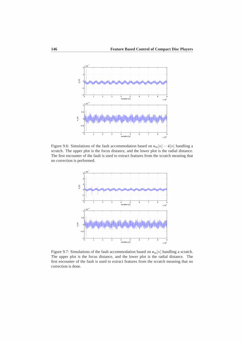
146 Feature Based Control of Compact Disc Players
0 1 2 3 4 5 6 7 8 9
x 104
−2
−1
0
1
2x 10
−7
e f [n]
samples [n]
0 1 2 3 4 5 6 7 8 9
x 104
−1
−0.5
0
0.5
1x 10
−8
e r [n]
samples [n]
Figure 9.6: Simulations of the fault accommodation based onem[n] − e[n] handling ascratch. The upper plot is the focus distance, and the lower plot is the radial distance.The first encounter of the fault is used to extract features from the scratch meaning thatno correction is performed.
0 1 2 3 4 5 6 7 8 9
x 104
−2
−1
0
1
2
3x 10
−7
e f [n]
samples [n]
0 1 2 3 4 5 6 7 8 9
x 104
−1
−0.5
0
0.5
1x 10
−8
e r [n]
samples [n]
Figure 9.7: Simulations of the fault accommodation based onem[n] handling a scratch.The upper plot is the focus distance, and the lower plot is the radial distance. Thefirst encounter of the fault is used to extract features from the scratch meaning that nocorrection is done.

9.5 Experimental results 147
The first method The second method
DP»0.64160.4318
– »1.90230.4468
–
Table 9.1: Table of the fault handling performanceDP, for both the feature based controlmethods. It can be seen that the first method is better than the second method onef [n],but the second method is marginally better onef [n]. This is properly due to the fact thatmeasurement noises are relatively larger compared with the faults in the radial signalsthan in the focus signals.
9.5 Experimental results
The next step is to verify the algorithm on the experimental test setup, see Chapter 3.1.In this experimental work only CDs with one scratch has been used, in order to avoidbook keeping of the surface faults. However, this scratch has not been included in thetraining set of the algorithm. The scratch has also been classified to be contained inClass 1 - small scratches. Due to limitations in the computer power in the test setup,the algorithm was not used on both focus and radial loops at the same time. For thesame reason only the second method was tested with success. It has not been possibleto implement the first method due to real-time problems. However, the other parts of themethod suggested in this thesis have previously been validated by experimental workpresented in this thesis. A scheme combining all these scheme parts is assumed to givebetter experimental results as simulations indicates.In the first experiment the fault was detected by the use of prediction of the time local-isation based on the location of the previous faults. A clear advantage of this approachis that the fault can be removed from the beginning of the surface fault, which shouldresult in an almost entire removal of the scratch from the measuredem[n]. This ap-proach is highly sensible to non-deterministic variations in the length of the revolutionsin samples, (variations mean additional variations to the increase in the duration of onerevolution with one sample for each third revolution due to the spiral shaped track onthe disc). Analyses of the experimental data show that the variations in the duration ofthe revolutions vary with up to 5 samples from one revolution to the next one. Such alarge variation will result in problems for the fault correction algorithm. It might causethe use of the algorithm to result in a poorly performance than if the correction was notperformed. The same analyses of the experimental data also show that the length of sur-face faults do not change from revolution to revolution, this fact is of large importancelater on.A couple of experiments were performed using the prediction of the fault location ap-proach. These experiments resulted as presumed in a good fault correction when loca-tion prediction is correct, and on the other hand resulted in a very poorly fault correctionwhen this prediction did fail, see Fig. 9.8.In Fig. 9.8 the potentials of the algorithm are shown at the 4th and the 5th encounter
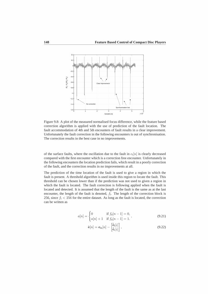
148 Feature Based Control of Compact Disc Players
0 1 2 3 4 5 6
x 104
−1.6
−1.4
−1.2
−1
−0.8
−0.6
−0.4
−0.2
0
0.2
0.4
Samples [n]
(D1−
D2)/
(D1+
D2)
No correction
Clear improvement
Synchronisation lost
Figure 9.8: A plot of the measured normalised focus difference, while the feature basedcorrection algorithm is applied with the use of prediction of the fault location. Thefault accommodation of 4th and 5th encounters of fault results in a clear improvement.Unfortunately the fault correction in the following encounters is out of synchronisation.The correction results in the best case in no improvements.
of the surface faults, where the oscillation due to the fault inef [n] is clearly decreasedcompared with the first encounter which is a correction free encounter. Unfortunately inthe following encounters the location prediction fails, which result in a poorly correctionof the fault, and the correction results in no improvements at all.
The prediction of the time location of the fault is used to give a region in which thefault is present. A threshold algorithm is used inside this region to locate the fault. Thisthreshold can be chosen lower than if the prediction was not used to given a region inwhich the fault is located. The fault correction is following applied when the fault islocated and detected. It is assumed that the length of the fault is the same as at the lastencounter, the length of the fault is denoted,fl . The length of the correction block is256, sincefl < 256 for the entire dataset. As long as the fault is located, the correctioncan be written as
a[n] =
{0 if fd[n − 1] = 0,a[n] + 1 if fd[n − 1] = 1.
, (9.21)
e[n] = em[n] −[ˇef [ι]ˇer[ι]
], (9.22)

9.5 Experimental results 149
0 1 2 3 4 5 6
x 104
−0.7
−0.6
−0.5
−0.4
−0.3
−0.2
−0.1
0
0.1
0.2
0.3
Samples [n]
(D1−
D2)/
(D1+
D2)
The first correction
First encounter
Figure 9.9: A plot of the measured normalised focus difference while the correctionalgorithm is applied with the use of fault detection. It is clear to see that the correctionresults in a limitation of the influence from the fault on the measured normalised focusdifference.
where
ι = ((256 − lf) div (2)) + a. (9.23)
In Fig. 9.9 an example of this method is illustrated. The first encounter of the scratchis not corrected, but instead used to train the algorithm. In the encounters following thefirst one a clear improvement is achieved. It can also be seen more clear from the zoomon the 1st and 5th encounter of the fault, see Fig. 9.10.Following the algorithm was tested on the radial servo loop, which is known as beingmore sensitive to faults than the focus servo. This test was performed with the CD-player in test mode, see Chapter 3.1. An example of the algorithm handling a scratchcan be seen in Fig. 9.11. The nominal controller actually looses the radial tracking inthe example in Fig. 9.11 which can be seen by the heavy oscillations. However, whenthe correction algorithm is applied the radial tracking is not lost. A zoom on the 2nd and4th encounter of the fault is shown in Fig. 9.12.These experimental results show that a limited version of feature based fault correctionalgorithm, which is proposed in this chapter, gives a clear improvement of the perfor-mance handling the surface faults, at least in the case of the tested scratches. The entirealgorithm might even give better results, as simulations indicates. In Section 3.2 it wasstated: “The main problem to solve in this Ph.D project is to handle surface faults thatare impossible to handle by normally used methods.” The feature based control schemehas not been tested on such surface faults, due to some practical problems. However, it

150 Feature Based Control of Compact Disc Players
0 50 100 150 200 250 300 350 400 450−0.7
−0.6
−0.5
−0.4
−0.3
−0.2
−0.1
0
0.1
0.2
0.3
Samples [n]
(D1−
D2)/
(D1+
D2)
1st encounter5th encounter
SurfaceFault
Figure 9.10: A zoom on the 1st and 5th encounter of the fault shown in Fig. 9.9.
0 0.5 1 1.5 2 2.5 3 3.5 4 4.5
x 104
−0.3
−0.2
−0.1
0
0.1
0.2
0.3
0.4
0.5
Samples [n]
(S1−
S2)/
(S1+
S2)
Encounters without corrections
First encouter with corrections
Figure 9.11: A plot of the measured normalised radial difference while the fault correc-tion algorithm is applied with the use of thresholding in a predicted interval. It is clear tosee that the fault correction algorithms result in limitation of the influence from the faulton the approximateder[n], when the correction algorithm is applied at the 4th encounterof the fault. It can be seen that if no correction is applied the fault forces the OPU intoheavy oscillations, which are avoided when the correction algorithm is used.
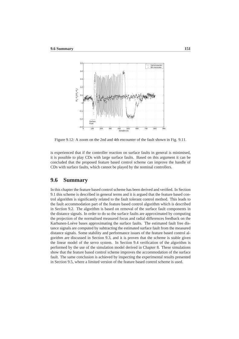
9.6 Summary 151
0 100 200 300 400 500 600 700 800 900−0.3
−0.2
−0.1
0
0.1
0.2
0.3
0.4
0.5
Samples [n]
(S1−
S2)/
(S1+
S2)
2nd encounter4th encounter
Surface Fault
Figure 9.12: A zoom on the 2nd and 4th encounter of the fault shown in Fig. 9.11.
is experienced that if the controller reaction on surface faults in general is minimised,it is possible to play CDs with large surface faults. Based on this argument it can beconcluded that the proposed feature based control scheme can improve the handle ofCDs with surface faults, which cannot be played by the nominal controllers.
9.6 Summary
In this chapter the feature based control scheme has been derived and verified. In Section9.1 this scheme is described in general terms and it is argued that the feature based con-trol algorithm is significantly related to the fault tolerant control method. This leads tothe fault accommodation part of the feature based control algorithm which is describedin Section 9.2. The algorithm is based on removal of the surface fault components inthe distance signals. In order to do so the surface faults are approximated by computingthe projection of the normalised measured focus and radial differences feedback on theKarhunen-Loève bases approximating the surface faults. The estimated fault free dis-tance signals are computed by subtracting the estimated surface fault from the measureddistance signals. Some stability and performance issues of the feature based control al-gorithm are discussed in Section 9.3, and it is proven that the scheme is stable giventhe linear model of the servo system. In Section 9.4 verification of the algorithm isperformed by the use of the simulation model derived in Chapter 8. These simulationsshow that the feature based control scheme improves the accommodation of the surfacefault. The same conclusion is achieved by inspecting the experimental results presentedin Section 9.5, where a limited version of the feature based control scheme is used.


Chapter 10
Conclusion
This thesis deals with different aspects on how to improve the playability of the CD-players for CDs with surface faults, such as scratches and fingerprints. The suggestedmethod called feature based control, is in its essential an active fault tolerant controlmethod combined with time-frequency based signal processing. In the following thecontributions of the thesis are summarised and reviewed. This summary is followed bysome suggestions for future work, which is based on this project.
10.1 Conclusions
In this thesis fault tolerant control is used for a class of systems, where repetitive sensorfaults occur. This class of systems contains applications in the field of optical discplayers playing discs with surface faults. A scheme is developed which is adapted to aspecific CD-player. However, it is expected that this scheme can be used in general forfor system in the considered class of systems. This novel method is based on a number ofmethods and results which are achieved in the areas of: modelling of the optical system,design of residuals, fault detection, time-frequency based feature extraction, simulationsand feature based control.
• A model of the optical detector system is derived. This model includes the opticalcross-couplings between focus and radial detectors. Outside the normal operationrange of the focus and radial loops this optical mapping is strongly non-linear.The derived model is validated based on measurements. The validation showsthat the model is well suited for control purposes. However, the derived modelhas some numerical problems which is handled by approximating the functions inthe model by the use of cubic splines.
• In most industrial players either the focus or the radial sum signal is used as theresidual for detection of the surface faults. Unfortunately the focus sum signal
153

154 Conclusion
depends the radial distance and the radial sum signal depends on the focus dis-tance. Instead a couple of decoupled residuals are derived based on a model ofthe surface faults. These residuals are compared with the normally used residualson some real scratches and show a clear improvement of the localisation of thesescratches.
• The previously mentioned residuals can only be computed if the inverse map ofthe combined optical and fault model is used. This mapping is only locally definedcomputational method is suggested by the use of Newton-Raphson’s method anda Kalman estimator. In addition the Kalman estimator gives an estimate of focusand radial distances during a surface fault.
• The decoupled residuals are the starting point for the fault detection and localisa-tion. Three methods are designed to locate and detect the surface faults based onthese residuals. Two time-frequency based methods are designed, and as well asan extension of the normally used threshold. The two time-frequency based meth-ods are Fang’s algorithm, and a wavelet packet filter. These two methods has thedrawback that one filter cannot be used to detect all surface faults. Instead a set offilters are needed in order to locate all surface faults by the use of these waveletpacket filters. However, the extended threshold method gives a clear improvementof the fault detection and localisation in all tested cases.
• Time-frequency based methods are used to extract features from the detected sur-face faults. The extracted features are classification of the surface faults, (this clas-sification separates the faults in smaller classes thereby more adapted fault han-dling can be achieved), and approximating coefficients in the Karhunen-Loève ba-sis. These features are used for two purposes, simulation of the surface fault, andto accommodate them by removal of the surface faults component from the mea-surements. The classification and approximation are verified on test data whichare not used in the data set to train the classification and approximation.
• In order to test how well a controller can handle a surface fault, a simulator of sur-face faults is designed by using the approximating Karhunen-Loève basis. Thesesynthesised surface fault are simulation of specific surface faults, but contained inthe given class of surface faults. The simulation model is completed by the use ofstandard models of focus and radial servos combined with the new optical modeldeveloped in this thesis.
• The feature based control method is designed to handle the surface faults. Bysubtracting the estimation of surface fault from focus and radial distance signals.These cleaned distance signals are subsequently fed to the nominal controllers.The nominal controller can be used without reacting to the surface faults. Themethod is in this design limited to handle only one scratch on the played disc. Thismethod is validated through simulations and experimental tests, where a simpli-fied version was tested with good results. In these simulations and tests the often
10.2 Future work 155
used PID-controllers were used in order to illustrate the fact that the feature basedcontrol scheme accommodates the surface faults without using special controllers.
All these novel contributions lead to a method which can improve the performance ofthe focus and radial servos in a CD-player, playing a CD with a surface faults, such asscratches and fingerprints. The experimental work has been focused on the scratchesand the method is as a consequence adapted to the scratches. The method as one hasnot been tested by the experimental tests. However, the parts of the methods have beentested by experimental work with good results. The feature based control method usedon a CD-player has both in simulations and experimental tests (a simple version) shownimprovements in the handling of the tested scratches.
10.2 Future work
Several ideas and problems have appeared but not covered during this Ph.D project.These problems and ideas will be described in the following.
• This feature based method is designed to a specific CD-player. It would be very in-teresting to extend the method to other optical disc players. The obviously choiceof the first player to extend it to, is the DVD-player, but also the new high densitystandards are of high interest. In addition it would also be interesting to adapt themethod to high speed drives.
• The fault classification and estimation in the proposed method are based on alimited training set of measured surface faults. This means that surface faultsexist which are poorly represented by the fault classes and approximating bases.This will result in a poor handling of the surface faults. One way to improve thisis to expand the training set.
• Only a small number of bases were tested in the fault classification method, otherbases might be even more discriminating than the one used. Another possibilityis to combine different libraries of bases, meaning that a set of base vectors fromdifferent bases are chosen.
• The large number of surface faults can be handled in an other way. The firstencounter of the fault is used to train an approximating Karhunen-Loève basis ofthe surface fault. This method has an even larger potential if the CD-player hasthe storage capacity to store the features of the surface faults on all the CDs it hasplayed. It is probably necessary, due to limited storage capacity, to store only themost problematic surface faults on a number of CDs.
• It might also be useful to adapt the fault detection filters to the classified faults.This would make the use of the time-frequency based filters possible, since thesefilters tend to be too narrow-banded to be used for all faults.

156 Conclusion
• It was not possible to implement the entire algorithm due to real-time problems inthe test setup. As a consequence it would be a good idea to design a faster versionof the method. One of the problems is the computation of the inverse map. Somestudies have indicated that it is possible to determine the inverse of the modelmapping locally, which can remove all the iterative computations.
• The method as it is now can only handle one surface fault at each CD. As a con-sequence it would be a good idea to implement a book keeping algorithm whichmakes it possible to handle more than one surface fault per CD.
• Another possible usage of this method is the reconstruction of data on severedamaged discs, where playback is not possible even though the suggested methodis used. It might be possible to retrieve the data from the disc by changing therotational speed of the disc in addition to the use of the suggested method.
• A final interesting topic to investigate further is how surface faults influence focusand radial distance measurements. This might be achieved by studying diffractivetheory.

Bibliography
[Aangenent, 2002] Aangenent, W. (2002). The modeling and control of the sledge sy-stem in the Beosound 3000. Technical report, Department of Control Engineering,Institut of Electronic Systems, Aalborg University, Denmark.
[Andersen and Karlsson, 2000] Andersen, B. and Karlsson, R. (2000). Regulering afoptisk pickup i cd-afspiller. Master’s thesis, Department of Control Engineering,Institute of Electronic systems, Aalborg University, Denmark. In Danish.
[Andersen et al., 2001] Andersen, P., Pedersen, T., Stoustrup, J., and Vidal, E. (2001).Method for improved reading of digital data disc. International patent, no. WO02/05271 A1.
[AOSRA, 2003] AOSRA (2003). Taiwan joins optical-disk IP fray.http://www.eetimes.com/sys/news/OEG20030324S0032.
[Basseville and Nikiforov, 1993] Basseville, M. and Nikiforov, I. (1993).Detection ofabrupt changes : theory and application. Prentice Hall, first. edition.
[Blanke et al., 2003] Blanke, M., Kinnaert, M., Lunze, J., and Staroswiecki, M. (2003).Diagnosis and Fault-tolerant Control. Springer.
[Bouwhuis et al., 1985] Bouwhuis, W., Braat, J., Huijser, A., Pasman, J., van Rosmalen,G., and Schouhamer Immink, K. (1985).Principles of Optical Disc Systems. AdamHilger Ltd.
[Braat et al., 2002] Braat, J., Dirksen, P., and Jansen, A. (2002). Diffractive readout ofoptical discs. In Török, P. and Kao, F.-J., editors,Optical Imaging and MicroscopyTechniques and Advanced Systems. Springer, first edition.
[Chait et al., 1994] Chait, Y., Soo Park, M., and Steinbuch, M. (1994). Design andimplementation of a QFT controller for a compact disc player. InProceedings of the1994 American Control Conference, Baltimore, Maryland, USA.
[Chen and Patton, 1991] Chen, J. and Patton, R. J. (1991).Robust model-based faultdiagnosis for dynamic systems. Kluwer academic publishers, first edition.
157
158 BIBLIOGRAPHY
[Coifman and Saito, 1994] Coifman, R. R. and Saito, N. (1994). Constructions of localorthonormal bases for classification and regression.Comptes Rendus de l’Académiedes Sciences de Paris, 319(2):191–196.
[Coifman and Wickerhauser, 1992] Coifman, R. R. and Wickerhauser, M. V. (1992).Entropy-based algorithm for best basis selection.IEEE Transaction on InformationTheory, 38(2):713–718.
[Dettori, 2001] Dettori, M. (2001).LMI techniques for control - with application toa Compact Disc player mechanism. PhD thesis, Technische Universiteit Delft, TheNetherlands.
[Dettori et al., 1999] Dettori, M., Valk, P., and Scherer, C. (1999). Digital implemen-tation of a mixed objectives mimo controller for a compact disc player using a mul-tiprocessor system. InProceedings of the 1999 American Control Conference, SanDiego, CA, USA.
[Dokur et al., 1999] Dokur, Z., Ölmez, T., and Yazgan, E. (1999). Comparison of dis-crete wavelet and fourier transforms for ecg beat classification.Electronics Letters,35(18):1502 – 1504.
[Dötch et al., 1995] Dötch, G., Smakman, T., Van den Hof, P., and Steinbuch, M.(1995). Adaptive repetitive control of a compact disc mechanism. InProceedingsof the 34th IEEE Conference on Decision and Control, New Orleans, LA ,USA.
[Draijer et al., 1992] Draijer, W., Steinbuch, M., and Bosgra, O. (1992). Adaptive con-trol of the radial servo system of a compact disc player.Automatica, 28(3):455–462.
[Dzanovic and Lauritsen, 2003] Dzanovic, H. and Lauritsen, K. (2003). Modellering afslædesystemet i et cdm12 løbeværk. Technical report, Department of Control Engi-neering, Institute of Electronic Systems, Aalborg University, Denmark. In Danish.
[Dötsch, 1998] Dötsch, H. (1998).Identification of Control Design with Application toa Compact Disc Mechanism. PhD thesis, Technische Universiteit Delft, The Nether-lands.
[ECMA, 2001] ECMA (2001).Standard ecma-267: 120mm dvd read-only-disk. Stan-dard.
[Fang, 1994] Fang, X. (1994). Automatic phoneme segmentation of continuous speechsignals. Preprint.
[Filardi, 2003] Filardi, G. (2003).Robust control design strategies applied to a DVD-video player. PhD thesis, Université Joseph Fourier, Grenoble, France.
[Filardi et al., 2003] Filardi, G. Sename, O., Besaçon-Voda, A., and Schroder, H.(2003). RobustH∞ control of a dvd drive under parametric uncertainties. InPro-ceedings of European Control Conference 2003, Cambridge, UK.

BIBLIOGRAPHY 159
[Flury, 1997] Flury, B. (1997).A first course in multivariate statistics. Springer Verlag,first edition.
[Frank, 1990] Frank, P. M. (1990). Fault diagnosis in dynamic systems using analyti-cal and knowledge-based redundancy. a survey and some new results.Automatica,26(3):459–474.
[Franklin et al., 1998] Franklin, G. F., Powell, J. D., and Workman, M. (1998).Digitalcontrol of dynamic systems. Addison Wesley, third edition.
[Fujiyama et al., 1998] Fujiyama, K., Tomizuka, M., and Katayama, R. (1998). Digitaltracking controller design for cd player using disturbance observer. InInternationalWorkshop on Advanced Motion Control, Coimbra, Portugal.
[Gamba and Marazzi, 1997] Gamba, P. and Marazzi, A. (1997). A comparison betweenwavelet and threshold detection of rain patterns from radar data. InSixth InternationalConference on Image Processing and Its Applications, Dublin, Ireland.
[Gertler, 1998] Gertler, J. J. (1998).Fault Detection and Diagnosis in EngineeringSystem. Marcel Dekker, Inc.
[Goossens and Odgaard, 2003] Goossens, H. and Odgaard, P. (2003). Optical disc servothat is robust for defects. European patent application no. 03104587.5.
[Hearns and Grimble, 1999] Hearns, G. and Grimble, M. (1999). Limits of performanceof an optical disk drive controller. InProceedings of the 1999 American ControlConference, San Diego, CA, USA.
[Heertjes and Sperling, 2003] Heertjes, M. and Sperling, F. (2003). A nonlinear dy-namic filter to improve disturbance rejection in optical storages drives. InProceed-ings of the 42nd IEEE Conference on Decision and Control, Maui, HI, USA.
[Heertjes and Steinbuch, 2004] Heertjes, M. and Steinbuch, M. (2004). Stability andperformance of a variable gain controller with application to a dvd storage drive.Automatica, 40(4):591–602.
[Hess-Nielsen and Wickerhauser, 1996] Hess-Nielsen, N. and Wickerhauser, M.(1996). Wavelets and time-frequency analysis.Proceedings of The IEEE, 84(4):523– 540.
[Hitachi, Ltd. et al., 2002] Hitachi, Ltd., LG Electronics Inc., Matsushita Electric In-dustrial Co., Ltd, Pioneer Corporation, Royal Philips Electronics, Samsung Elec-tronics Co., Ltd., Sharp Corporation, Sony Corporation, and Thomson Multimedia(2002). Large capacity optical disc video recording format “blu-ray disc” established.Press Release: http://www.sony.net/SonyInfo/News/Press/200202/02-0219E/.

160 BIBLIOGRAPHY
[Hnili cka et al., 2002] Hnilicka, B., Besançon-Voda, A., Filardi, G., and Schroeder, H.(2002). Modelling the focus error characteristic of a dvd player. InProceedings ofthe 2002 IEEE International Conference on Control Applications, Glasgow, Scotland,UK.
[Honguh, 2002] Honguh, Y. (2002). Readout signal analysis of optical disk base donan approximated vector diffraction theory. InInternational Symposium on OpticalMemory and Optical Data Storage Topical Meeting 2002, Waikoloa, HI, USA.
[Huang et al., 1999] Huang, Y., Mathur, P., and Messner, W. (1999). Robustness analy-sis on a high bandwidth disk drive servo system with an instrumented suspension. InProceedings of the 1999 American Control Conference, San Diego, CA, USA.
[Jensen and la Cour-Harbo, 2001] Jensen, A. and la Cour-Harbo, A. (2001).Ripples inMathematics - The Discrete Wavelet Transform. Springer, Berlin Heidelberg, Ger-many, first edition.
[Johnson and Wichern, 2002] Johnson, R. and Wichern, D. (2002).Applied Multivari-ate Statistical Analysis. Prentice Hall, 5th edition.
[Khargonekar et al., 1985] Khargonekar, P., Poolla, K., and Tannenbaum, A. (1985).Robust control of linear time-invariant plants using periodic compensation.IEEETransaction on Automatic Control, 30(11):1088 – 1096.
[Kojima and Wakabayashi, 1997] Kojima, T. and Wakabayashi, K. (1997). Three-dimensional analysis of light-beam scattering from pit and emboss marks of opticaldisk models. In1997. IEEE. Digest. Antennas and Propagation Society InternationalSymposium, Montreal, Que., Canada.
[Kraut et al., 2004] Kraut, S., Andersen, R., and Krolik, J. (2004). A generalizedkarhunen-loeve basis for efficient estimation of tropospheric refractivity using radarclutter. IEEE Transaction on Signal Processing, 52(1):48–60.
[la Cour-Harbo, 2002] la Cour-Harbo, A. (2002).Robust and Low-Cost Active Sensorsby means of Signal Processing Algorithms. PhD thesis, Department of Control Engi-neering, Aalborg University. ISBN: 87-90664-13-2.
[Lee, 1998] Lee, C. H. (1998).Robust repetitive control and application to a CD player.PhD thesis, Trinity Hall Cambridge University.
[Li et al., 1995] Li, C., Zheng, C., and Tai, C. (1995). Detection of ecg characteristicpoints using wavelet transforms.IEEE Transactions on Biomedical Engineering,42(1):21 – 28.
[Li and Tsao, 1999] Li, J. and Tsao, T.-C. (1999). Rejection of repeatable and non-repeatable disturbances for disk drive actuators. InProceedings of the 1999 AmericanControl Conference, San Diego, CA, USA.

BIBLIOGRAPHY 161
[Lopez et al., 1994] Lopez, J. E., Tenney, R. R., and Deckert, J. C. (1994). Fault detec-tion and identification using real-time wavelet feature extraction. InProceedings ofthe IEEE-SP International Symposium on Time-Frequency and Time-Scale Analysis,Philadelphia, PA, USA.
[Mallat, 1989] Mallat, S. (1989). A theory for multiresolution signal decomposition:The wavelet representation.IEEE Transaction on Pattern Analysis and Machine In-telligence, 11(7):674 – 693.
[Mallat, 1999] Mallat, S. (1999).A wavelet tour of signal processing. Academic Press,second. edition.
[Mokhtari et al., 2002] Mokhtari, H., Karimi-Ghartemani, M., and Iravani, M. R.(2002). Experimental performance evaluation of a wavelet-based on-line voltage de-tection method for power quality applications.IEEE Transaction on Power Delivery,17(1):161 – 172.
[Moon et al., 1996] Moon, J., Lee, M., and Jin Chung, M. (1996). Track-followingcontrol for optical disk drives using an iterative learning scheme.IEEE Transactionson Consumer Electronics, 42(2):192–198.
[Odgaard et al., 2003a] Odgaard, P., Stoustrup, J., Andersen, P., and Mikkelsen, H.(2003a). Detection of surface defects and servo signal restoration for a compact discplayer. Submitted for journal publication.
[Odgaard et al., 2003b] Odgaard, P., Stoustrup, J., Andersen, P., and Mikkelsen, H.(2003b). Extracting focus and radial distances, fault features from cd player sensorsignals by use of a kalman estimator. InProceedings of the 42nd IEEE Conferenceon Decision and Control, Maui, Hawaii, USA.
[Odgaard et al., 2003c] Odgaard, P., Stoustrup, J., Andersen, P., and Mikkelsen, H.(2003c). Modelling of the optical detector system in a compact disc player. InPro-ceedings of the 2003 American Control Conference, Denver, USA.
[Odgaard et al., 2004a] Odgaard, P., Stoustrup, J., Andersen, P., and Mikkelsen, H.(2004a). Fault detection for compact disc players based on redundant and non-linearsensors. InProceedings of American Control Conference 2004, Boston, MA, USA.
[Odgaard et al., 2004b] Odgaard, P., Stoustrup, J., Andersen, P., and Wickerhauser, M.(2004b). Joint best basis wavelet packet based detection of surface faults on compactdisc. Submitted for publication.
[Odgaard et al., 2003d] Odgaard, P., Stoustrup, J., Andersen, P., Wickerhauser, M., andMikkelsen, H. (2003d). Matlab source for simulation of cd player with surface de-fects. www.control.aau.dk/∼odgaard/software/CDsim. The link includes matlab anddata files for download, which are needed for using the simulation software.

162 BIBLIOGRAPHY
[Odgaard et al., 2004c] Odgaard, P., Stoustrup, J., Andersen, P., Wickerhauser, M., andMikkelsen, H. (2004c). A fault tolerant control scheme for cd players to handlesurface defects. Submitted for journal publication.
[Odgaard et al., 2004d] Odgaard, P., Stoustrup, J., Andersen, P., Wickerhauser, M.,and Mikkelsen, H. (2004d). A simulation model of focus and radial servos incompact disc players with disc surface defects. InProceedings of the 2004 IEEECCA/ISIC/CACSD, Taipei, Taiwan.
[Odgaard et al., 2004e] Odgaard, P., Stoustrup, J., Andersen, P., Wickerhauser, M., andMikkelsen, H. (2004e). Stability of close loop controlled repetitive periodic systems.Submitted for publication.
[Odgaard and Wickerhauser, 2003] Odgaard, P. and Wickerhauser, M. (2003). Discrim-ination between different kind of surface defects on compact discs. To appear inProceedings of IEEE IECON 2004.
[Odgaard and Wickerhauser, 2004] Odgaard, P. and Wickerhauser, M. (2004). Timelocalisation of surface defects on optical discs. InProceedings of the 2004 IEEECCA/ISIC/CACSD, Taipei, Taiwan.
[Ouyang and Wickerhauser, 1993] Ouyang, H. and Wickerhauser, M. V.(1993). WSQ – the FBI/Yale/Los Alamos [W]avelet-packet [S]calar[Q]uantization fingerprint compression algorithm, for Windows 3.1 or higher.http://www.math.wustl.edu/∼victor/software/wsq/index.html.
[Parameswariah and Cox, 2002] Parameswariah, C. and Cox, M. (2002). Frequencycharacteristics of wavelets.IEEE Transactions on Power Delivery, 17(3):800 – 804.
[Patton et al., 1989] Patton, R., Frank, P., and Clark, R. (1989).Fault Diagnosis inDynamic Systems - Theory and Application. Prentice Hall International.
[Philips, 1994] Philips (1994).Product specification: Digital servo processor DSIC2,TDA1301T. Philips Semiconductors, Eindhoven, The Netherlands.
[Philips and Sony Corporation, 1991] Philips and Sony Corporation (1991). Compactdisc digital audio. Red book, which is non public standard, but most of the relevantspecifications can be seen in other literature e.g. [Stan, 1998].
[Pohlmann, 1992] Pohlmann, K. (1992).The Compact Disc Handbook. Oxford Uni-versity Press, 2nd edition.
[Reed and Solomon, 1960] Reed, I. and Solomon, G. (1960). Polynomial codes overcertain finite fields.Journal of the Society for Industrial and Applied Mathematics,8(2):300–304.

BIBLIOGRAPHY 163
[Saito, 1994] Saito, N. (1994).Local Feature Extraction and Its Applications Using aLibrary of Bases. PhD thesis, Yale University.
[Saito, 1998] Saito, N. (1998). The least statically-dependent basis and its applications.In Conference Record of the Thirty-Second Asilomar Conference on Signals, Systems& Computers, Pacific Grove, CA, USA.
[Schneiders, 2001] Schneiders, M. (2001). Wavelets in control engineering. Master’sthesis, Eindhoven University of Technology. Dynamics and Control Technology,Faculty of Mechanical Engineering, Eindhoven University of Technology.
[Stan, 1998] Stan, S. G. (1998).The CD-ROM drive. Kluwer Academic Publishers.
[Steinbuch et al., 1992] Steinbuch, M., Schoostra, G., and Bosgra, O. (1992). Robustcontrol of a compact disc player. InProceedings of the 31st IEEE Conference onDecision and Control, Tucson, Arizona, USA.
[Steinbuch et al., 1994] Steinbuch, M., van Groos, P., Schootstra, G., and Bosgra, O.(1994). Multivariable control of compact disc player using DSPs. InProceedings ofthe American Control Conference, Baltimore, Maryland, USA.
[Strang and Nguyen, 1997] Strang, G. and Nguyen, T. (1997).Wavelets and FilterBanks. Wellesley- Cambridge Press, Wellesley, MA, revised edition.
[Sureshbabu and Farrell, 1999] Sureshbabu, N. and Farrell, J. A. (1999). Wavelet-basedsystem identification for nonlinear control.IEEE Transactions on Automatic Control,44(2):412 – 417.
[Toliyat et al., 2003] Toliyat, H. A., Abbaszadeh, K., Rahimian, M. M., and Olson, L. E.(2003). Rail defect diagnosis using wavelet packet decomposition.IEEE Transactionof Industry Application, 39(5):1454 – 1461.
[Toshiba Corporation and NEC Corporation, 2002] Toshiba Corporation and NEC Cor-poration (2002). Toshiba and NEC Jointly Propose Next Generation High Capacity,Blue-laser DVD Format. http://www.nec.co.jp/press/en/0208/2901.html.
[Ulfarsson et al., 2002] Ulfarsson, M., Benediktsson, J., and Sveinsson, J. (2002).Wavelet feature extraction and genetic feature selection for multisource data. InIGARSS ’02. 2002 IEEE International Geoscience and Remote Sensing Symposium,Toronto, Canada.
[van Helvoirt et al., 2004] van Helvoirt, J., Leenknegt, G. A. L., Steinbuch, M., andGoossens, H. J. (2004). Classifying disc defects in optical disc drives by using time-series clustering. InProceedings of the American Control Conference 2004, Boston,MA, USA.
164 BIBLIOGRAPHY
[Vetterli and Kovacevic, 1995] Vetterli, M. and Kovacevic, J. (1995).Wavelets and sub-band coding. Prentice Hall PTR, Saddle River, NJ, first edition.
[Vidal et al., 2001a] Vidal, E., Andersen, P., Stoustrup, J., and Pedersen, T. (2001a). Astudy on the surface defects of a compact disk. InProceedings of the 2001 IEEEInternational Conference on Control Applications, Mexico City, Mexico.
[Vidal et al., 2001b] Vidal, E., Hansen, K., Andersen, R., Poulsen, K., Stoustrup, J.,Andersen, P., and Pedersen, T. (2001b). Linear quadratic control with fault detectionin compact disk players. InProceedings of the 2001 IEEE International Conferenceon Control Applications, Mexico City, Mexico.
[Vidal et al., 1998] Vidal, E., Shøien, H., and Rasmussen, J. (1998). Focus control of theoptical pick-up in a cd player. Master’s thesis, Department of Control Engineering,Institute of Electronic systems, Aalborg University, Denmark.
[Vidal et al., 2001c] Vidal, E., Stoustrup, J., Andersen, P., Pedersen, T., and Mikkelsen,H. (2001c). Open and closed loop parametric system identification in compact diskplayers. InACC2001, Arlington, Virginia.
[Vidal Sánchez, 2003] Vidal Sánchez, E. (2003).Robust and Fault Tolerant control ofCD-players. PhD thesis, Department of Control Engineering, Aalborg University.ISBN: 87-90664-15-9.
[Warner Bros, 2002] Warner Bros (2002). Dvd production: Factions debate hd-dvd.Press news: http://www.medialinenews.com/issues/2002/september/dvd_10.shtml.
[Weerasooriya and Phan, 1995] Weerasooriya, S. and Phan, D. (1995). Discrete-timeLQG/LTR design and modeling of a disk drive actuator tracking servo system.IEEETransactions on Industrial Electronics, 42(3):240–247.
[Wesfreid and Wickerhauser, 1999] Wesfreid, E. and Wickerhauser, M. V. (1999). Vo-cal command signal segmentation and phoneme classification. In Ochoa, A. A., edi-tor, Proceedings of the II Artificial Intelligence Symposium at CIMAF 99. Institute ofCybernetics, Mathematics and Physics (ICIMAF), Habana, Cuba.
[Wickerhauser, 1994a] Wickerhauser, M. (1994a).Adapted Wavelet Analysis from The-ory to Software. A K Peters, Ltd., 1st edition.
[Wickerhauser, 1991] Wickerhauser, M. V. (1991). Fast approximate factor analysis.In Silbermann, M. J. and Tagare, H. D., editors,Curves and Surfaces in ComputerVision and Graphics II, volume 1610 ofSPIE Proceedings, pages iii + 395, Boston.SPIE.
[Wickerhauser, 1994b] Wickerhauser, M. V. (1994b). Large-rank approximate princi-pal component analysis with wavelets for signal feature discrimination and the inver-sion of complicated maps.Journal of Chemical Information and Computer Science,34(5):1036–1046.

BIBLIOGRAPHY 165
[Wisniewski and Stoustrup, 2001] Wisniewski, R. and Stoustrup, J. (2001). General-ized H2 control synthesis for periodic systems. InAmerican Control Conference2001, Arlington, Virginia, USA.
[Wook Heo and Chung, 2002] Wook Heo, J. and Chung, J. (2002). Vibration and noisereduction of an optical disk drive by using a vibration absorber.IEEE Transactionson Consumer Electronics, 48(4):874 – 878.
[Xiangxun, 2002] Xiangxun, C. (2002). Wavelet-based detection, localization, quantifi-cation and classification of short duration power quality disturbances. InIEEE PowerEngineering Society Winter Meeting, New York, NY, USA.
[Yao et al., 2001] Yao, L., Wang, A.-M., and Cheng, Y.-F. (2001). Track seeking hy-brid fuzzy controller for the compact disc player. InThe 10th IEEE InternationalConference on Fuzzy Systems, Melbourne, Australia.
[Ye et al., 2002] Ye, H., Wang, G., and Ding, S. X. (2002). Integrated design of faultdetection system in time-frequency domain.IEEE Transaction on Automatic Control,47(2):384–390.
[Ye et al., 2003] Ye, H., Wang, G., and Ding, S. X. (2003). A new fault detection ap-proach based on parity relation and stationary wavelet transform. InProceedings ofthe American Control Conference 2003, Denver, CO, USA.
[Ye et al., 2004] Ye, H., Wang, G., and Ding, S. X. (2004). A new parity space ap-proach for fault detection based on stationary wavelet transform.IEEE Transactionon Automatic Control, 49(2):281–287.
[Yeh and Pan, 2000] Yeh, T.-J. and Pan, Y.-C. (2000). Modeling and identification ofopto-mechanical coupling and backlash nonlinearity in optical disk drives.IEEETransactions on Consumer Electronics, 46(1):105–115.
[Yen et al., 1992] Yen, J.-Y., Lin, C.-S., and Li, C-H. Chen, Y.-Y. (1992). Servo con-troller design for an optical disk drive using fuzzy control algorithm. InIEEE Inter-national Conference on Fuzzy Systems, San Diego, CA, USA.
[Yokoyama et al., 1994] Yokoyama, E., Nagasawa, M., and Katayama, T. (1994). Adisturbance suppression control system for car-mounted and portable optical diskdrives. IEEE Transactions on Consumer Electronics, 40(2):92–99.
[Zhou et al., 2002] Zhou, Y., Steinbuch, M., and Kostic, D. (2002). Estimator-basedsliding mode control of an optical disc drive under shock and vibration. InCCA02,Glasgow, Scotland, UK.
[Zhu et al., 1997] Zhu, S., Choo, F., K.S., L., Chan, C., and Kong, P. (1997). Servosystem control in digital video disc (dvd). InISCE ’97 - Proceedings of 1997 IEEEInternational Symposium on Consumer Electronics, Singapore, Singapore.


Appendix A
Electro-magnetic-mechanicalmodel
Contenious time models The focus electro-magnetic-mechanical model is
ef(s)uf(s)
= 1.5497 · 105 · 3.5869s2 + 5.8741 · s + 3.6148 · 104
(A.1)
The radial electro-magnetic-mechanical model is
er(s)ur(s)
= 1.652 · 106 · 0.6727s2 + 5.8741 · s + 9.7901 · 104
(A.2)
Extended discrite time models
Φ =
266666666664
0.9998 −1.033 0 0 0 0 0 02.857 · 10−5 1 0 0 0 0 0 0
0 0 0.9978 −0.03042 0 0 0 00 0 2.854 · 10−5 1 0 0 0 00 0 0 0 0.9998 −2.7969 0 00 0 0 0 2.8569 · 10−5 1.0000 0 00 0 0 0 0 0 0.9978 −0.03040 0 0 0 0 0 2.8541 · 10−5 1.0000
377777777775
,
(A.3)
Γ =
266666666664
5.7138 · 10−6 08.1628 · 10−11 0
0 00 00 5.7137 · 10−6
0 8.1628 · 10−11
0 00 0
377777777775
, (A.4)
Ψ =
266666666664
5.7138 · 10−7 08.1628 · 10−12 0
0 00 00 5.7137 · 10−7
0 8.1628 · 10−12
0 00 0
377777777775
, (A.5)
CCD =»0 2.2235 100.0000 0 0 0 0 00 0 0 0 0 2.2235 100.0000
–. (A.6)
167

Appendix B
Optical model
In this appendix is the identified parameters in optical model listed. All theparameters are adressed with their respective the part functions in the model:h1, h2, h3, h4, g1, g3, g4.
The identified parameters are not nescary the value of the physical parameters, sinceparameter identification do not find these physical parameters, but finds a set of param-eters which given a model output close to the measured signals. As a consequence thephysical units are left out in the tables A.1-A.4.
lu,0 lx,0 F R k0
0.0010 2.2698·10−17 0.0129 1.3604·10−6 1.3402·10−14
P r r0 b α1000 6.2917·10−11 9.8656·10−7 1.2788·10−6 3.6100·10−6
Table B.1: Identified parameters inh1(·) andh2(·).

169
r r0 b α6.2917·10−11 4.96191·10−7 1.7936·10−6 2.2161·10−6
Table B.2: Identified parameters inh3(·) andh4(·).
r bs ρpit ρland
4·10−7 3.7621·10−7 0.4291 1.6237
Table B.3: Identified parameters ing1(·).
B.0.1 Polynomials
The coefficients in the polynomials inh3(·) andh4(·) are
ph1 =
−929.0194599.1097730.0290−468.6936−170.5094124.29200.4108
−12.61543.60620.52750.0326
, ph2 =
−454.4608209.0713189.7289−107.010568.287761.9910
−44.20384.84595.6990−0.58670.0480
, (B.1)
where the polynomials are defined as:
pS1(x) = ph1(1) · x10 + ph1(2) · x9 + . . . + ph1(11), (B.2)
pS2(x) = ph2(1) · x10 + ph2(2) · x9 + . . . + ph2(11). (B.3)

170 Optical model
r bs ρpit ρland
4·10−7 9.0686·10−7 0.1094 0.4942
Table B.4: Identified parameters ing3(·) andg4(·).

Appendix C
Kalman estimators
The kalman gains are computed to be
M∞ =
166.7491 00.0631 0
−4.2311 · 10−14 03.0313 · 10−15 0
0 1.0432 · 103
0 0.14880 2.8887 · 10−13
0 −3.9815 · 10−14
, (C.1)
L∞ =
166.6535 00.0678 0
−4.2312 · 10−14 03.0301 · 10−15 0
0 1.0426 · 103
0 0.17860 2.8946 · 10−13
0 −3.9807 · 10−14
. (C.2)
171

Appendix D
Controllers
The normal focus PID-controller is
uf(z)ef(z)
=1476z2 − 2630z + 1159
z3 − 1.332z2 + 0.3598z − 0.02759(D.1)
The low-banded focus PID-controller is
uf(z)ef(z)
=1453z2 − 2618z + 1165
z3 − 1.332z2 + 0.3598z − 0.02759(D.2)
The normal radial PID-controller is
uf(z)ef(z)
=124.8z2 − 222.3z + 97.97
z3 − 1.332z2 + 0.3598z − 0.02759(D.3)
The low-banded radial PID-controller is
uf(z)ef(z)
=122.9z2 − 221.3z + 98.48
z3 − 1.332z2 + 0.3598z − 0.02759(D.4)