Aalborg Universitet Efficient Multicast in Next Generation Mobile Networks...
191
Aalborg Universitet Efficient Multicast in Next Generation Mobile Networks Wang, Haibo Publication date: 2008 Document Version Publisher's PDF, also known as Version of record Link to publication from Aalborg University Citation for published version (APA): Wang, H. (2008). Efficient Multicast in Next Generation Mobile Networks. Aalborg: Aalborg Universitet. General rights Copyright and moral rights for the publications made accessible in the public portal are retained by the authors and/or other copyright owners and it is a condition of accessing publications that users recognise and abide by the legal requirements associated with these rights. ? Users may download and print one copy of any publication from the public portal for the purpose of private study or research. ? You may not further distribute the material or use it for any profit-making activity or commercial gain ? You may freely distribute the URL identifying the publication in the public portal ? Take down policy If you believe that this document breaches copyright please contact us at [email protected] providing details, and we will remove access to the work immediately and investigate your claim. Downloaded from vbn.aau.dk on: May 24, 2019
Transcript of Aalborg Universitet Efficient Multicast in Next Generation Mobile Networks...

Aalborg Universitet
Efficient Multicast in Next Generation Mobile Networks
Wang, Haibo
Publication date:2008
Document VersionPublisher's PDF, also known as Version of record
Link to publication from Aalborg University
Citation for published version (APA):Wang, H. (2008). Efficient Multicast in Next Generation Mobile Networks. Aalborg: Aalborg Universitet.
General rightsCopyright and moral rights for the publications made accessible in the public portal are retained by the authors and/or other copyright ownersand it is a condition of accessing publications that users recognise and abide by the legal requirements associated with these rights.
? Users may download and print one copy of any publication from the public portal for the purpose of private study or research. ? You may not further distribute the material or use it for any profit-making activity or commercial gain ? You may freely distribute the URL identifying the publication in the public portal ?
Take down policyIf you believe that this document breaches copyright please contact us at [email protected] providing details, and we will remove access tothe work immediately and investigate your claim.
Downloaded from vbn.aau.dk on: May 24, 2019

Department of Electronic Systems
Efficient Multicast in Next Generation MobileNetworks
by
Haibo Wang, MSc
Dissertation
Presented to the International Doctoral School of Technology and Science,
Aalborg Universitet,
in Partial Fulfillment of the Requirements for the Degree of
Doctor of Philosophy
Aalborg Universitet
22 October 2008

Supervisors:
Hans-Peter Schwefel, Associate Professor, PhD, Aalborg University
Thomas Skjodeberg Toftegaard, PhD, TietoEnator, Aarhus
Assessment Committee:
Professor Tan Zhenhui, Beijing Jiaotong University, China
Professor Christoph Mecklenbräuker, Vienna University of Technology, Austria
Troels B. Sørensen, Associate Professor (chairman), Aalborg University
Moderator:
Tatiana Kozlova Madsen, Associate Professor, PhD, Aalborg University
Copyright c© October 2008 by
Haibo Wang
Aalborg University
Niels Jernes Vej 12
Aalborg Øst
Denmark
e-mail: [email protected]
All rights reserved by the author.
Printed in Aalborg, Denmark

iii
Haibo Wang

Dedicated to...
my family for their unconditional support


Abstract
The next generation mobile cellular networks are expected to transmit rich multi-
media services, which often require large transmission bandwidth, low delay and
the same content to be delivered to several users. Due to the broadcast nature of
radio transmission, the most efficient way to provide such services is to employ
wireless multicast. By sending one copy of the service content to several multi-
cast group members with a shared downlink channel, the bandwidth consumption
can be significantly reduced and the efficiency of using scarce radio resource can
be improved. On the other hand, the diversity of the channel conditions among
multiple receivers raise challenges to the radio resource management (RRM) al-
gorithm design for such a multicast channel. In this PhD project, a comprehensive
RRM study with both analytical and simulative approaches is fulfilled to explore
the tradeoff between spectral efficiency and reliability in this wireless multicast
channel.
First, a performance metric has been built to balance the multicast system
spectral efficiency and the user perceived Quality of Service (QoS). A simple
modulation rate adaptation scheme is proposed to maximize such metric in an
OFDMA-based multicast channel. Then the metric is simplified to reduce its sen-vi

vii
sitivity to its weight factors, and a more sophisticated modulation rate adaptation
algorithm is proposed to optimistically relax the instantaneous Bit Error Ratio
(BER) constraints based on the BER history of each multicast user. The proposed
algorithm has been evaluated in connection to other link adaptation schemes by
simulations, which shows significant spectral efficiency advantage under the given
QoS constraint.
To reveal the performance upper-boundary of multicast link adaptations in
general, an analytical model is built. The optimization problem is reformulated to
a constraint optimization problem with joint power and modulation rate adapta-
tion under flat- and block-fading Rayleigh channels. The optimal and suboptimal
adaptation approaches along different dimensions (power and modulation rate)
are derived from this analytical model, as well as the corresponding achievable
spectral efficiency values. The criteria of switching from uncash channel mode to
multicast channel mode is also revealed from the analytical results.
All these studies reveals that the worst channel state degrades the overall
multicast system performance, and this penalty increases as the multicast group
size grows. Automatic Repeat request (ARQ) can help to improve the overall
spectral efficiency under poor channel conditions, but facing scalability problems
in multicast. This dissertation proposes a cross-layer framework to jointly op-
timize Adaptive Modulation and Coding (AMC) and ARQ scheme, and adopts
packet-combining to solve the scalability problem under practical group size as-
sumptions.
In summary, this dissertation presents how RRM approaches can be em-
ployed to improve multicast spectral efficiency with reliability constraints. It re-Haibo Wang

viii
veals that violating the reliability constraint temporarily for the worst link can
improve the average spectral efficiency per user significantly, without sacrificing
the average reliability in long term. It is also proved that even though rate adapta-
tion alone can achieve similar performance as joint power and rate adaptation can
do if the data rate can be changed continuously, the latter still outperforms in more
realistic cases where only discrete data rates are available. Last but not the least,
cross-layer design with innovative multicast ARQ scheme can further exploit the
spectral efficiency and reliability trade-off if a certain delay is tolerable.
Aalborg Universitet

Dansk Resumé
Næste generations mobile netværk giver mulighed for transmission af avancerede
multimedie-services. Disse services kræver ofte en høj transmissions-båndbredde,
lav forsinkelse af trafik samt at de transmitterede data skal nå frem til flere mod-
tagere. Eftersom radiotransmissioner kan høres af flere modtagere samtidigt er
den mest effektive metode for udbydelse af sådanne services at benytte trådløs
multicast. En enkelt strøm af data kan sendes samtidigt til adskillige medlem-
mer af en multicast-gruppe gennem en delt downlink kanal. På denne måde kan
brugen af båndbredde reduceres betydeligt samtidig med at de begrænsede ra-
dioressourcer kan udnyttes mere effektivt. På den anden side oplever de enkelte
modtagere forskellige kanalforhold hvilket stiller udfordringer til designet af radio
resource management (RRM) algoritmer for multicast-kanaler. I dette PhD projekt
er gennemført et omfattende RRM studie hvor analytiske og simuleringsbaserede
fremgangsmåder danner grundlag for a studere afvejningen mellem spektral effek-
tivitet og pålidelighed i trådløse multicast-kanaler.
Initierende er en ydelsesparameter blevet defineret til at beskrive forholdet
mellem spektral effektivitet og Quality of Service (QoS) som brugeren oplever
den. For at maksimere denne parameter i en OFDM-baseret multicast kanal intro-ix

x
duceres en simpel modulationsrate adapteringsteknik. En simplificering af ydelses-
parameteren er blevet indført for at mindske dens følsomhed overfor egne in-
terne parametre. Efterfølgende er en mere sofistikeret modulationsrate adapter-
ingsteknik blevet introduceret der lemper kravene til den øjeblikkelige Bit Error
Ratio (BER) givet at den gennemsnitlige BER er inden for kravene. Ved brug af
simulering er den foreslåede algoritme blevet evalueret i forhold til andre link-
adapteringsteknikker. Målt på spektral effektivitet viser den foreslåede algoritme
en signifikant fordel under de benyttede QoS krav.
En analytisk model er blevet opstillet for at fastlægge en øvre grænse for den
mulige ydelse af multicast link-adaptering. Optimeringsproblemet er blevet om-
formuleret som et afgrænset optimeringsproblem der håndterer kombineret adapter-
ing af sendestyrke og modulationsrate under antagelse af en flat- og block-fading
Rayleigh kanal i et single-carriersystem. Baseret på den analytiske model er udledt
optimale og suboptimale adapteringsmetoder i forskellige dimensioner (sendestyrke
og moduleringsrate) samt tilhørende værdier for den opnåelige spektrale effek-
tivitet. Fra de analytiske resultater er også blevet udledt kriterier for at foretage et
skifte fra en unicast kanal til en multicast kanal.
De udførte studier viser at den, af en modtager, værst oplevede kanaltilstand
forringer den overordnede ydelse af multicast systemet. Denne forringelse forøges
når størrelsen af multicast-gruppen stiger. Automatisk Repeat reQuest (ARQ) kan
benyttes til a forbedre den overordnede spektrale effektivitet under dårlige kanal-
forhold, men med multicast kan dette give anledning til skaleringsproblemer. I
denne afhandling introduceres en cross-layer metode der muliggør kombineret op-
timering af Adaptive Modulation og Coding (AMC) og ARQ hvor Coding-teknikAalborg Universitet

xi
benyttes på pakkeniveau for a løse skaleringsproblemerne under realistiske an-
tagelser om gruppestørrelser.
Denne afhandling præsenterer hvordan RRM-teknikker kan anvendes til a
forbedre den spektrale effektivitet under multicast med pålidelighedskrav/QoS
krav. Det er vist hvordan en signifikant forbedring i spektral effektivitet kan opnås
ved at tillade midlertidige brud på pålidelighedkravene uden at det har betydning
for den gennemsnitlige pålidelighed på lang sigt. Under antagelse af en trinløs
indstilling af transmissionsraten kan rateadaptering alene, opnå lignende ydelse
som under kombineret transmissionsstyrke- og rateadaptering. Det er dog be-
vist hvordan sidstnævnte fremgangsmåde er bedre i realistiske tilfælde hvor kun
diskrete data rater er tilgængelige. Slutteligt skal fremhæves hvordan cross-layer
designet med den innovative multicast ARQ-teknik giver mulighed for at udnytte
afvejninger af spektral effektivitet og pålidelighed hvis en givet forsinkelse kan
tolereres.
Haibo Wang

Acknowledgments
First of all, I would like to express my heartiest gratitude to my PhD Supervisors,
Associate Prof. Hans-Peter Schwefel at Aalborg University and Thomas Skjode-
berg Toftegaard at TietoEnator. Since I met Hans as a master student in 2004, he
has always been encouraging me to follow my curiosity, to challenge my limit, and
to achieve the new height I had never imagine before. Whenever I have difficulties,
he has always been there for me. As my supervisor in TietoEnator, Thomas has
guided me to develop my competence in both the academia and in the industry.
He has inspired me with a broad version, combining both technology enthusiasm
and market sense. What I have learned from Hans and Thomas will always be a
great treasure in my future career.
Thanks to Assistant Prof. Persefoni Kyritsi. Whenever I have trouble on the chan-
nel and antenna issues, she has always helped me out with her clear picture of
knowledge and great patience. Also thanks to Associate Prof. Jon E. Johnsen for
verifying my mathematics model.
Thanks to Megumi Kaneko, Chenguang Lu, Guillaume Monghal, and many otherxii
ACKNOWLEDGMENTS xiii
fellow PhD students in our Electronic System Department for their support and
discussions, which have enriched my knowledge and inspired me during my en-
tire PhD project. Especially thanks to Jesper Grønbæk, my officemate and fellow
PhD student, who has made great efforts to translate the abstract of this disserta-
tion into the Dansk Resumé.
Thanks to Prof. Ye (Geoffrey) Li for hosting me in his lab as a visiting student in
Georgia Institute of Technology. This was a great experience and the cross-layer
design in my thesis was inspired during this visiting.
Thanks to all my friends I have met in Denmark and USA, and to all my friends
back in China.
No expressions can express my gratitude to my parents and my grandmother. Their
love and caring has always been supporting me and make me strong, though they
are far away from Denmark.
HAIBO WANG
Aalborg Universitet
October 2008
Haibo Wang

Contents
Abstract vi
Dansk Resumé ix
Acknowledgments xii
List of Figures xix
List of Tables xxii
Chapter 1 Introduction 1
1.1 Motivation . . . . . . . . . . . . . . . . . . . . . . . . . . . . . . 1
1.2 Problem Delimitation . . . . . . . . . . . . . . . . . . . . . . . . 4
1.2.1 Optimization Scenario . . . . . . . . . . . . . . . . . . . 4
1.2.2 Problem Statement . . . . . . . . . . . . . . . . . . . . . 8
1.2.3 Objectives and Scope of the Work . . . . . . . . . . . . . 9
1.3 Summary of the Contributions . . . . . . . . . . . . . . . . . . . 11
1.4 Organization of Thesis . . . . . . . . . . . . . . . . . . . . . . . 14xiv

CONTENTS xv
Bibliography 16
Chapter 2 Background 19
2.1 Wireless Channel Features . . . . . . . . . . . . . . . . . . . . . 19
2.1.1 Path-loss and Shadowing . . . . . . . . . . . . . . . . . . 20
2.1.2 Multipath Fading . . . . . . . . . . . . . . . . . . . . . . 21
2.1.3 Channel Fading versus Modulation . . . . . . . . . . . . 22
2.2 Orthogonal Frequency Division Multiplexing (OFDM) . . . . . . 24
2.2.1 OFDMA . . . . . . . . . . . . . . . . . . . . . . . . . . 28
2.2.2 OFDMA-Based Standards Groups . . . . . . . . . . . . . 30
2.3 Radio Resource Management (RRM) . . . . . . . . . . . . . . . 33
2.3.1 AMC and Power Adaptation . . . . . . . . . . . . . . . . 34
2.3.2 Water-Filling Principle . . . . . . . . . . . . . . . . . . . 35
2.3.3 ARQ . . . . . . . . . . . . . . . . . . . . . . . . . . . . 37
2.4 State-of-the-art . . . . . . . . . . . . . . . . . . . . . . . . . . . 40
2.4.1 OFDM link adaptation and multi-user diversity . . . . . . 40
2.4.2 Related work with multiple unicast users . . . . . . . . . 41
2.4.3 Related work with one multicast group . . . . . . . . . . 42
2.5 Summary . . . . . . . . . . . . . . . . . . . . . . . . . . . . . . 42
Bibliography 44
Chapter 3 Rate Adaptation for Mobile Multicast 51
3.1 Motivation . . . . . . . . . . . . . . . . . . . . . . . . . . . . . . 52
3.2 System Model and Assumptions . . . . . . . . . . . . . . . . . . 53
3.2.1 OFDMA . . . . . . . . . . . . . . . . . . . . . . . . . . 54Haibo Wang
xvi CONTENTS
3.2.2 Channel Model . . . . . . . . . . . . . . . . . . . . . . . 54
3.2.3 BER Approximations . . . . . . . . . . . . . . . . . . . . 55
3.3 Simulator Description . . . . . . . . . . . . . . . . . . . . . . . . 56
3.3.1 Simulation Scenario . . . . . . . . . . . . . . . . . . . . 56
3.3.2 System Level Simulator . . . . . . . . . . . . . . . . . . 57
3.4 Reward Function-Based Adaptation . . . . . . . . . . . . . . . . 58
3.4.1 Performance Evaluation Approach . . . . . . . . . . . . . 58
3.4.2 Different Adaption Strategies . . . . . . . . . . . . . . . 60
3.4.3 Numerical Result and Analysis . . . . . . . . . . . . . . . 63
3.4.4 Sub-Conclusion . . . . . . . . . . . . . . . . . . . . . . . 69
3.5 History-Based BER Threshold Adaptation . . . . . . . . . . . . . 70
3.5.1 Performance Evaluation Metric . . . . . . . . . . . . . . 70
3.5.2 Different Adaptation Strategies . . . . . . . . . . . . . . 71
3.5.3 Simulation Results and Analysis . . . . . . . . . . . . . . 75
3.5.4 Sub-Conclusion . . . . . . . . . . . . . . . . . . . . . . . 79
3.6 Conclusion . . . . . . . . . . . . . . . . . . . . . . . . . . . . . 79
Bibliography 82
Chapter 4 Multi-Dimensional Optimization with Analytical Model 85
4.1 Motivation . . . . . . . . . . . . . . . . . . . . . . . . . . . . . . 85
4.2 Single-Carrier System Model . . . . . . . . . . . . . . . . . . . . 87
4.3 Problem Formulation . . . . . . . . . . . . . . . . . . . . . . . . 89
4.4 Solutions with Continuous Rate Adaptation . . . . . . . . . . . . 92
4.4.1 Adaptation Schemes . . . . . . . . . . . . . . . . . . . . 92Aalborg Universitet

CONTENTS xvii
4.4.2 Numerical Result of Case Studies . . . . . . . . . . . . . 96
4.5 Solutions with Discrete Rate Adaptation . . . . . . . . . . . . . . 103
4.5.1 Discrete Rate and Optimal Power (DRSopt) . . . . . . . . 103
4.5.2 Discrete Rate and Constant Power (DRSc) . . . . . . . . 107
4.5.3 Numerical Results of Case Studies . . . . . . . . . . . . . 108
4.6 Conclusion and Future Work . . . . . . . . . . . . . . . . . . . . 110
Bibliography 112
Chapter 5 Cross Layer Design for Multicast 114
5.1 Motivation . . . . . . . . . . . . . . . . . . . . . . . . . . . . . . 114
5.2 Related Work . . . . . . . . . . . . . . . . . . . . . . . . . . . . 116
5.3 Cross-Layer System Model . . . . . . . . . . . . . . . . . . . . . 119
5.4 Multicast ARQ with Packet-Combining . . . . . . . . . . . . . . 123
5.4.1 Two Users Group . . . . . . . . . . . . . . . . . . . . . . 124
5.4.2 N Users Group . . . . . . . . . . . . . . . . . . . . . . . 125
5.5 AMC Strategies . . . . . . . . . . . . . . . . . . . . . . . . . . . 127
5.6 Evaluation Methods . . . . . . . . . . . . . . . . . . . . . . . . . 129
5.7 Case Study I: N = 2 . . . . . . . . . . . . . . . . . . . . . . . . 130
5.7.1 Performance Analysis in Close-Form Expression . . . . . 130
5.7.2 Numerical Results . . . . . . . . . . . . . . . . . . . . . 135
5.8 Case Study II: N ≥ 2 . . . . . . . . . . . . . . . . . . . . . . . . 137
5.8.1 Numerical Results . . . . . . . . . . . . . . . . . . . . . 138
5.9 Conclusion and Future Work . . . . . . . . . . . . . . . . . . . . 142
Bibliography 146Haibo Wang

xviii CONTENTS
Chapter 6 Conclusion 148
6.1 Summary . . . . . . . . . . . . . . . . . . . . . . . . . . . . . . 148
6.2 Outlook . . . . . . . . . . . . . . . . . . . . . . . . . . . . . . . 151
Appendix A Additional Results of the Cross-Layer Strategies 153
Appendix B List of Abbreviations 157
Appendix C List of Math Notations and Symbols 161
Aalborg Universitet

List of Figures
1.1 General Scenario . . . . . . . . . . . . . . . . . . . . . . . . . . 5
1.2 Multicast Transmitter and Receivers . . . . . . . . . . . . . . . . 6
2.1 Wireless Channel Propagation Phenomena . . . . . . . . . . . . . 20
2.2 OFDM with 8 Sub-Carriers . . . . . . . . . . . . . . . . . . . . . 25
2.3 An OFDM Transceiver Diagram . . . . . . . . . . . . . . . . . . 26
2.4 OFDMA with Static FDMA Scheme . . . . . . . . . . . . . . . . 28
2.5 OFDMA with Fully Dynamic Frequency-Time Block Allocation . 29
2.6 OFDMA Sub-Channel Modes . . . . . . . . . . . . . . . . . . . 30
2.7 Illustration of "Water-Filling" Solution . . . . . . . . . . . . . . . 36
3.1 An OFDMA Adjacent Sub-Channel for Multicast . . . . . . . . . 53
3.2 BER Approximations for BPSK and MQAM . . . . . . . . . . . 56
3.3 Simulator Diagram . . . . . . . . . . . . . . . . . . . . . . . . . 58
3.4 Reward under E(SNR) = 28dB . . . . . . . . . . . . . . . . . . 64
3.5 Throughput and satisfaction ratio (E(SNR) = 28dB) . . . . . . . 65
3.6 Cumulative Distribution Function (CDF) of SNR, Mean=28dB,STD=11dB 66
3.7 SNR CDF, Mean=35dB,STD=11dB . . . . . . . . . . . . . . . . 68xix

xx LIST OF FIGURES
3.8 Reward under E(SNR)=35dB . . . . . . . . . . . . . . . . . . . . 68
3.9 Satisfaction Ratio under E(SNR) = 35dB . . . . . . . . . . . . 69
3.10 Best Reward AM with Heuristic BER Constraint . . . . . . . . . 73
3.11 Reward Comparison, E(SNR)=20dB . . . . . . . . . . . . . . . . 75
3.12 Average BER Comparison, E(SNR)=20dB . . . . . . . . . . . . . 76
3.13 Impacts of δ Settings on Adaptive BER Algorithm, E(SNR)=20dB 77
3.14 Impacts of θ1 Settings on Adaptive BER Algorithm, E(SNR)=20dB 78
3.15 Spectrum Efficiency of AM Strategies, E(SNR)=20dB . . . . . . 79
4.1 S/S versus min~γ . . . . . . . . . . . . . . . . . . . . . . . . . 97
4.2 k versus min~γ . . . . . . . . . . . . . . . . . . . . . . . . . . 98
4.3 Spectrum Efficiency per User in Rayleigh Channel . . . . . . . . 99
4.4 Impact of Cut-Off SNR (Rayleigh PDF, Mean=10dB) . . . . . . . 101
4.5 Linear Power Adaptation, Impact of Slope β on Spectrum Efficiency102
4.6 Integration Region of 2 UE, D-Rate . . . . . . . . . . . . . . . . 106
4.7 Optimal Power Schemes with Discrete Modulation Rate . . . . . 107
4.8 Per User Spectral Efficiency of All Adaptation Schemes . . . . . . 108
5.1 Multicast System Model with Cross-Layer Design . . . . . . . . . 120
5.2 Multicast Packet Loss Pattern for 2 UEs . . . . . . . . . . . . . . 124
5.3 Integration Region of 2 UEs, D-Rate . . . . . . . . . . . . . . . . 132
5.4 Rate Regions of Max-SINR Strategy . . . . . . . . . . . . . . . . 134
5.5 Performances of Different Adaptation Strategies, N = 2 . . . . . 136
5.6 Performances of AMC-ARQ Strategies VS Group Size, SINR =
10dB . . . . . . . . . . . . . . . . . . . . . . . . . . . . . . . . . 139Aalborg Universitet

LIST OF FIGURES xxi
5.7 Spectral Efficiencies of S1 with Different ARQs, SINR = 10dB . 141
A.1 Performances of AMC-ARQ Strategies VS Group Size, SINR =
5dB . . . . . . . . . . . . . . . . . . . . . . . . . . . . . . . . . 155
A.2 Performances of AMC-ARQ Strategies VS Group Size, SINR =
15dB . . . . . . . . . . . . . . . . . . . . . . . . . . . . . . . . . 156
Haibo Wang

List of Tables
2.1 OFDM Parameters in Mobile WiMAX [11] . . . . . . . . . . . . 32
3.1 Selected OFDMA Parameters . . . . . . . . . . . . . . . . . . . . 54
3.2 Important System Assumptions . . . . . . . . . . . . . . . . . . . 57
3.3 The Best Local Reward Algorithm . . . . . . . . . . . . . . . . . 62
3.4 SNR Thresholds for BER < 10−3 . . . . . . . . . . . . . . . . . 63
3.5 BER Estimations . . . . . . . . . . . . . . . . . . . . . . . . . . 67
3.6 The Best Local Reward Algorithm with Fixed BER Threshold . . 72
3.7 Adaptive BER Threshold Algorithm . . . . . . . . . . . . . . . . 74
5.1 Transmission AMC Modes with Convolutional-Coded Modulation 121
xxii

Chapter 1
Introduction
1.1 Motivation
At present, wireless multimedia applications like multi-party video conferences,
Video on Demand, or on-line mobile gaming are demanding high bandwidth while
at the same time posing real-time requirements on the communication infrastruc-
ture. On the other hand, a large part of the content in these applications are com-
mon information required by a group of users. Hence to allow multiple users to
share the same network resource (wired network resource or radio resource) via
Multicast/Broadcast is highly attractive in providing current and future wireless
multimedia services.
Broadcast and multicast are the two modes of point-to-multipoint (PTM)
communications. In Broadcast, the same content is delivered to all receivers within
the transmission range from the sender. Known examples are radio and TV ser-
vices, which are broadcasted over the air (either terrestrial or via satellite) and over
cable networks. In Multicast, on the other hand, each content are solely delivered
to users who have joined a particular multicast group. Normally, a multicast group
is a group of users interested in a certain kind of content, for example, sports,1

2 Chapter 1. Introduction
news, cartoons. A multicast- enabled network ensures that the content is solely
distributed over those links that are serving receivers which belong to the corre-
sponding multicast group. In large scale networks like the Internet, the available
content to be delivered are so diversified and the content senders and intended
receivers are distributed so far apart that broadcast is nearly impossible. Hence
multicast is the main concern of this dissertation.
Basically, wireless multicast can be done in either infrastructure-based mo-
bile networks or Ad-Hoc mobile networks. In infrastructure-based networks like
Global System for Mobile Communications (GSM) and Universal Mobile Telecom-
munications Systems (UMTS), Mobile Terminals (MTs) communicate with a base
station (BS) connecting to a backbone networks, which can help one MT to com-
municate with any other MT, fixed phone or Internet server anywhere. An ad-hoc
network is a self-organized network made up of a group of wireless mobile hosts
[1], where each host has to forward data for others due to the limited transmission
range of each mobile host. Such type of networks are usually designed for spe-
cific purpose, e.g, the battlefield networks, sensor networks. Whereas the wireless
multimedia content requiring multicast are usually provided by servers located in
infrastructure-based networks. That is, this dissertation only covers wireless mul-
ticast in infrastructure-based networks.
Wireless multicast has been drawing a lot of attention from both industry and
academia, i.e, UMTS Multimedia Broadcast and Multicast Service (MBMS) is a
framework designed by the Third Generation Partnership Project (3GPP) to extend
IP multicast to current 3G mobile networks [2, 3]. However, there are still many
open issues to solve in both the fixed backbone part and the radio cell part in orderAalborg Universitet

1.1 Motivation 3
to fully adopt multicast in mobile networks. In the backbone side, the problems
posed by mobility include: (a) the movement of the multicast source, if the content
sender is also a MT; (b) the movement of the multicast group members, thus the
multicast routing topology (namely the multicast tree) needs to be reconfigured
quickly; (c) data transmission reliability during hand-over, to avoid packet drop
or enable lost data recovery; (d) signalling overhead due to frequently changed
multicast tree topology and membership. In the radio cell side, challenges are
mainly upon the radio resource management.
Radio Resource Management (RRM) is the system level control of radio
transmission characteristics in wireless communication systems [4]. RRM in-
cludes strategies and algorithms controlling transmit power, channel allocation,
handover criteria, modulation schemes, error-control-coding schemes [7]. The
objective is to utilize the limited radio spectrum resources and radio network in-
frastructure as efficiently as possible. RRM considers multi-user system capacity
issues, rather than just point-to-point link capacity.
Though the problems of multicast on the wired network part have been in-
vestigated extensively [7, 8, 9, 10, 11, 12, 13], the challenges on the air interface
part have not been discussed thoroughly. Multicast problems on the air interface
are as interesting as those in the wired network part, and the reason is two-fold:
• Multicasting in air interface is very challenging since the wireless transmis-
sion is highly error-prone due to different fading phenomena and user mobil-
ity. The radio resources from a transmitter serving its receivers have to be
limited to control the interferences to receivers served by other transmitters.
Even though the radio resource management approaches have been fully de-Haibo Wang

4 Chapter 1. Introduction
veloped for Unicast mobile receivers, they may not be the right solutions for
multicast mobile users.
• The wireless transmission is broadcasting in its nature, therefore the mul-
ticasting on the air interface can utilize such nature to save the scarce ra-
dio resource. In the infrastructure-based networks today such as UMTS, the
downlink radio resource (from base station to mobile terminals) is “scarce”
due to the limitation enforced by the interference problem. By multicasting
the same content in a common channel to multiple receivers rather than uni-
casting via multiple channels, not only radio resources are saved but also the
interferences among multiple channels are reduced.
Therefore, this dissertation focus on the wireless multicast performance optimiza-
tion on the air interface with RRM approaches.
1.2 Problem Delimitation
1.2.1 Optimization Scenario
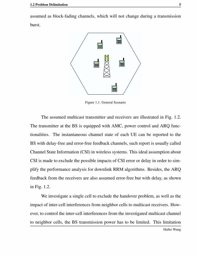
This dissertation assumes a single cell mobile system as depicted in Fig. 1.1, where
a BS located in the center and N users randomly distributed in this hexagonal cell.
The N users are all members of a multicast group, and there is a common downlink
channel dedicated to the multicast service demand by these users. The multicast
signal is sent to different User Equipments (UEs) within the same transmission
burst but experiencing different channel conditions due to, e.g., their different dis-
tance to the BS and different surroundings. The users are moving only within the
cell hence no handover is considered. The channel conditions of every users areAalborg Universitet
1.2 Problem Delimitation 5
assumed as block-fading channels, which will not change during a transmission
burst.
Figure 1.1: General Scenario
The assumed multicast transmitter and receivers are illustrated in Fig. 1.2.
The transmitter at the BS is equipped with AMC, power control and ARQ func-
tionalities. The instantaneous channel state of each UE can be reported to the
BS with delay-free and error-free feedback channels, such report is usually called
Channel State Information (CSI) in wireless systems. This ideal assumption about
CSI is made to exclude the possible impacts of CSI error or delay in order to sim-
plify the performance analysis for downlink RRM algorithms. Besides, the ARQ
feedback from the receivers are also assumed error-free but with delay, as shown
in Fig. 1.2.
We investigate a single cell to exclude the handover problem, as well as the
impact of inter-cell interferences from neighbor cells to multicast receivers. How-
ever, to control the inter-cell interferences from the investigated multicast channel
to neighbor cells, the BS transmission power has to be limited. This limitationHaibo Wang

6 Chapter 1. Introduction
will be reflected in either average power constraint or the resulted average Signal-
to-Noise-Ratio (SNR) or Signal-to-Interference-and-Noise-Ratio (SINR) settings,
depending on the investigation methods applied in each chapter of optimization
proposals. The common scenario and system assumptions in Fig. 1.1 and Fig. 1.2
Transmitter
AMC controllerARQ
controller& buffer
InputBuffer
Wirelessfading
channels
Data
Power controller
Channelestimator
Receiver
Channelestimator
Receiver
…
OutputData
OutputData
ARQ request
CSI feedback
UE 1
UE N
Figure 1.2: Multicast Transmitter and Receivers
will be narrowed down to address more specific issues in the following chapters.
Resource resource management (RRM) includes a wide range of radio re-
source allocation and adaptation approaches, namely access control, bandwidth
allocation and scheduling, link adaptation (LA) (including rate and power adap-
tation), ARQ, hand-over, etc. In the general scenario and assumptions of this
dissertation, the single cell and single group assumption means that access control
and handover are out of our scope. The rest RRM approaches will be reviewed in
the context of OFDM based next generation mobile systems in Chapter 2.
The ultimate target of network performance optimization is to achieve user
satisfaction by conveying applications successfully. QoS is a collective of serviceAalborg Universitet

1.2 Problem Delimitation 7
performances reflecting the degree of satisfaction of a user on a service [6], which
can be quantitatively evaluated with parameters like transmission data rate, delay,
jitter, error ratio (in bit error ratio or packet error ratio). Contemporary research
in multicast link adaptations mainly focuses on maximizing the system spectral
efficiency alone, but often neglect discussing the impact of their approaches upon
the user perceived QoS in different service categories. Our work, on the other
hand, optimizes the system performance from QoS perspective, specifically for
realtime multimedia services.
Considering the most-used QoS metrics for a multicast video-streaming ser-
vice in a mobile network, data rate and error ratio are largely effected by the air
interface, while the delay and jitter are impacted by many factors from physical
layer, network layer up to application layer. For data rate and error ratio, com-
paring to the scarce of radio resource and error-prone feature of radio network,
the wired backbone networks, often based on optical transmission facilities, are
bandwidth-sufficient and can provide nearly errorless transmission. Delay and jit-
ter, however, could happen anywhere in the wired networks due to the bursty na-
ture of data traffics, and need to be controlled with end-to-end approaches. There-
fore, our optimization mainly concerns average data rate and error ratio per user
in the radio cell. One may argue that link level ARQ on the air interface also intro-
duces delay for retransmissions, but if the error ratio in the wireless transmission
is effectively controlled, the probability that retransmission is required will be too
small to be the main cause of user perceived delay and jitter.
Haibo Wang
8 Chapter 1. Introduction
1.2.2 Problem Statement
The problems of multicast optimization in a single cell system are mainly caused
by two factors, the diversity of channel conditions among all group members, and
the time-varying nature of the worst link.
1.2.2.1 Channel Diversity of Users
In a cell, different MTs experience different channel conditions. When each of
them can be assigned a dedicated channel as in uncash case, the BS can allo-
cate/schedule radio resources like time-slots, carrier frequencies or antennas for
the user who has the best channel condition at the moment, and the radio resource
can be adapted to be optimal for this user’s channel condition. This is called
multi-user diversity. Whereas in multicast, the same content to different users with
different channel conditions has to be transmitted in the common channel simulta-
neously, hence such benefit of diversity-based scheduling is lost. In this situation,
it is impossible to achieve the optimal radio resource allocation or adaptation for
each group member at the same time, thus the optimization effort has to be com-
promised for the benefit of the whole group. Without scheduling and handover
options, multicast RRM reduces to mainly Link Adaptation (LA) approaches, e.g.
Adaptive Modulation and Coding (AMC), power control, Automatic Repeat re-
quest (ARQ), etc.
In a system with AMC, the modulation and coding formats are changed to
match the current received signal quality, i.e, the users with high SNR or SINR
are typically assigned higher-order modulations and high coding rates (e.g., 64-
Quadrature Amplitude Modulation (64-QAM) with rate-3/4 convolutional cod-Aalborg Universitet

1.2 Problem Delimitation 9
ing), whereas the users with low SNR or SINR are assigned low modulation-order
and/or low code rate (e.g., Quadrature Phase-Shift Keying (QPSK) and 1/2 con-
volutional coding). With power control, the power of the transmitted signal is
adjusted to meet a target signal quality at the receiver [14]. ARQ is an error
control method for data transmission, where the transmitter will know whether
a packet has been received correctly by getting acknowledgment messages from
the receiver, or timeouts. If a packet or frame is known to be lost, the transmitter
with ARQ function usually re-transmits the frame/packet. More details about link
adaptation methods will be described in chapter 2.
1.2.2.2 Time-varying of the Worst Link
If the same QoS standard (i.e, BER or PER) had to be achieved for all group
members, the worst link condition among users will limit the spectral efficiency
of the whole group. Intuitively multicast LA can be adapted to the worst link in
the group during a transmission burst. However, the wireless link conditions are
highly time-varying due to user mobility and channel fading phenomena, and each
receiver could be in poor channel conditions at some time. The larger the group,
the higher will be the probability that one or several users are in very bad link
conditions. Hence the LA strategy for the worst link may keep the data rate low
for large multicast group size [9].
1.2.3 Objectives and Scope of the Work
To this end, the focus of this PhD project is to optimize radio resources manage-
ment approaches in providing B3G/4G multicast services on the air interface. TheHaibo Wang

10 Chapter 1. Introduction
challenges within this optimization work include
• Efficient use of radio resources for multi-cast traffic:
New power and AMC schemes need to be proposed as existing Uncash-
oriented link adaptation schemes cannot be suitable for multicast services. As
analyzed in the problem statement, existing uncash power control and AMC
schemes cannot match the different channel conditions of group members si-
multaneously. Hence multicast group-based performance metric need to be
defined and power and AMC need to be designed to optimize such metric.
• QoS Provisioning/Reliable multi-cast schemes
It is a challenge how to provide QoS for multiple users in the same group
under different channel conditions. For the concerned QoS metric, to im-
prove average data rate per user matches the RRM goal to maximize the sys-
tem performance in terms of average spectral efficiency, bits/s/Hz; while the
BER/PER are posing reliability requirements to the wireless system. In wire-
less systems there exists a tradeoff between spectral efficiency and reliability.
I.e., under a given signal quality, transmission with higher modulation-order
and coding rate will result in higher data rate but with more errors than the
transmission with low modulation-order and coding rate. Hence the former
achieves better spectral efficiency but less reliability, while the latter achieves
better reliability with less spectral efficiency, roughly speaking. In multicast,
since the reliability will be limited by the worst channel condition, the trade-
off between reliability and spectral efficiency will be even more significant.
• Switch between Point-to-Point (PTP) and Point-to-Multipoint (PTM)
The switch between PTP and PTM communication modes in order to opti-Aalborg Universitet

1.3 Summary of the Contributions 11
mize spectral efficiency may depend on the number of multicast group mem-
bers and their distance to BS. I.e, when the group size is small and the channel
conditions of the users are highly diversified, it is arguable whether to adopt
multicast with a common channel or uncash with multiple dedicated chan-
nels.
• Diversity approaches to enhance Multicast efficiency or reliability
Transmit or receive diversity techniques can enhance the spectral efficiency
and/or the reliability in wireless fading channels, such as time domain diver-
sity like Automatic Retransmission request (ARQ), spatial domain diversity
like Multiple Input Multiple Output (MIMO). It is an open issue how to uti-
lize these diversities for multicast. E.g, ARQ schemes is usually considered
non-scalable if the number of receivers is large [2]. If ARQ is going to be
employed in multicast, the scalability problem has to be solved in the first
place.
As the scenario description and problem formulation have stated, scheduling and
handover are out of the scope of this dissertation. New optimization schemes are
proposed and evaluated with both simulation and analytical approaches.
1.3 Summary of the Contributions
The contributions in multicast RRM in mobile cellular systems are:
Utility-based adaptive modulation strategies A utility metric named Reward-
ing function is build to balance the system multicast performance and the
user perceived Quality of Service (QoS). A simple multicast modulation rateHaibo Wang

12 Chapter 1. Introduction
adaptation scheme is proposed to maximize such metric in an OFDMA sin-
gle cell setting. Then the metric is simplified to reduce its sensitivity to the
metric parameters, and a more sophisticated modulation rate adaptation algo-
rithm with history-based adaptive BER threshold is proposed and evaluated.
By using this algorithm the multicast performance of the user group is signif-
icantly improved compared to other link adaptation strategies.
Optimal and sub-optimal joint power and rate adaptation solutions To reveal
the performance upper-boundary of link adaptation approaches in general, an
analytical model is built. The focus of this analytical model is the joint power
and rate adaptations, hence the optimization problem was simplified to a con-
straint optimization problem. The advantages and disadvantages of adapta-
tion approaches along different dimensions (power and modulation rate) are
discussed based on this analytical model. The criteria of switching from un-
cash channel mode to multicast channel mode is also discussed according to
the analytical results.
Cross-layer design model An innovative solution where AMC and ARQ schemes
are jointly designed within a cross-layer framework. Packet-combining schemes
are proposed using packet level ’XOR’ operations to reduce the retransmis-
sion times, so that the scalability problem of multicast ARQs can be solved.
An average-PER-based (average over instantaneous group PERs) rate adap-
tation algorithm is developed to exploit more spectral efficiency gain given
ARQ exists. The numerical results shows that the joint design of the average-
PER-based rate adaptation and the optimal packet-combining ARQ achieve
the best spectral efficiency in the selected evaluation scenario, and success-Aalborg Universitet
1.3 Summary of the Contributions 13
fully keep the residual PER constraint at the same time. The results also
reveal that the gain of cross-layer design over non-cross-layer design with the
same rate adaptation strategy is stable under different ARQ schemes.
These contributions have been presented in the following publications.
• H. Wang, D. Prasad, X. Zhou, J. M. Llorente, F. Delawarde, G. Coget, P.
Eggers and H. P. Schwefel, “Improved Channel Allocation and RLC block
scheduling for Downlink traffic in GPRS,” in Proc. IEEE 61st Semiannual Ve-
hicular Technology Conference (VTC’05 Spring), Stockholm, Sweden, May
2005.
• H. Wang, D. Prasad, O. Teyeb and H. P. Schwefel, “Performance Enhance-
ments of UMTS networks using end-to-end QoS provisioning,” in Proc. In-
ternational Wireless Summit(IWS’05), Aalborg, Denmark, Sept. 2005.
• H. Wang, H. P. Schwefel and T. T. Nielsen, “Adaptive Modulation for a
Downlink Multicast Channel in OFDMA systems,” in Proc. IEEE Wireless
and Networking Conference (WCNC’07), HongKong, China, Mar. 2007.
• H. Wang, H. P. Schwefel and T. S. Toftegaard, “History-based Adaptive Mod-
ulation for a Downlink Multicast Channel in OFDMA systems,” in Proc.
IEEE Wireless and Networking Conference (WCNC’08), Las Vegas, USA,
Mar. 2008.
• H. Wang, H. P. Schwefel and T. S. Toftegaard, “The Optimal Joint Power and
Rate Adaptation for Mobile Multicast: A Theoretical Approach,” in Proc.
IEEE Sarnoff Symposium, Princeton, USA, Mar. 2008.Haibo Wang

14 Chapter 1. Introduction
• H. Wang, H. P. Schwefel and T. S. Toftegaard, “Mobile Multicast: the Opti-
mal Power and Rate Adaptations in a Unified View,” in preparation.
• H. Wang, H. P. Schwefel and T. S. Toftegaard, “A Cross-layer Design for
Mobile Multicast with Packet-Combining ARQ,” in preparation.
1.4 Organization of Thesis
The thesis is organized as follows:
Chapter 2 introduces the background knowledge related to our multicast RRM
problems, from wireless channel features to available RRM options in the
chosen multicast scenario.
Chapter 3 investigates the data rate adaptation problem in an OFDMA system.
The studied OFDMA system model and simulator are first described, and
then the proposed optimization metric as well as rate adaptation strategies are
explained, finally the simulation results are presented and discussed.
Chapter 4 analyzes the theoretical optimal performance and corresponding power
and rate adaptation solutions. It starts with formulating the problem into a
constrained optimization problem to maximize the per user spectral efficiency
under average power and instantaneous BER constraints. Then the problem
is solved with Lagrange methods and the results are analyzed with differ-
ent parameter settings. It is revealed that the constant power and continuous
rate adaptation can perform nearly as good as the optimal joint power and
rate adaptation scheme, but much more simple than the latter; whereas when
the available data rates are discrete, the performance of the optimal powerAalborg Universitet

1.4 Organization of Thesis 15
scheme outperforms the constant power scheme significantly. Another result
in this chapter is that it is always more efficient to switch to multicast mode
whenever there are more than one user requiring the same service, under in-
dependent and identical-distributed (i.i.d) channels.
Chapter 5 presents a framework to apply cross-layer design method in multicast
RRM. Both the AMC scheme and ARQ are optimized to maximize the overall
spectral efficiency. The performance is derived with an analytical model in
combination with Monte-Carlo method. The scalability problem of multicast
ARQ is solved with packet combining for different group sizes.
Chapter 6 concludes the dissertation and proposes guidelines for future work.
Haibo Wang

Bibliography
[1] T. Imielinski and H. F. Korth, Mobile Computing, Kluwer Academic Publish-
ers, 1996.
[2] 3GPP TS 23.246, “Multimedia Broadcast/Multicast Service; Architecture and
Functional Description Networks (PDN)”.
[3] 3GPP TR 23.846 6.1.0, “Multimedia Broadcast/Multicast Service (MBMS);
Architecture and functional description”, release 6, Dec. 2002.
[4] J. Zander, S-L Kim, M. Almgren and O. Queseth, Radio Resource Manage-
ment for Wireless Networks, Artech House Publishers, 2001.
[5] G. L. Stüber, Principles of Mobile Communication, 2nd ed., Kluwer Academic
Publishers, 2001.
[6] ITU-D SG 2 and ITC, Teletraffic Engineering Handbook,
http://www.tele.dtu.dk/teletraffic/handbook/telehook.pdf
[7] T. G. Harrison, C. L. Williamson, W. L. Mackrell and R. B. Bunt, “Mo-
bile multicast(MoM) protocol: multicast support for mobile hosts,” in Proc.
16

BIBLIOGRAPHY 17
ACM/IEEE International Conference on Mobile Computing and Networking,
pp. 151-160, Budapest, Hungary, Sept. 1997.
[8] C. R. Lin and C. J. Chung, “Mobile reliable multicast support in IP networks,”
in Proc. IEEE ICC 2000, vol. 3, pp. 1421-1425, New Orleans, USA, Jun. 2000.
[9] W. Jia, W. Zhou and J. Kaiser, “Efficient algorithm for mobile multicast using
anycast group,” in IEE Proc. Commum., vol. 148, no. 1, pp. 14-18, Feb. 2001.
[10] M. Hauge and Ø. Kure, “Multicast in 3G Networks: Employment of Existing
IP Multicast Protocols in UMTS,” IEEE WoWMoM’02, Atlanta, USA, Sept.
2002.
[11] G. Leoleis, L. Dimopoulou, V. Nikas and I. S. Venieris, “Mobility Manage-
ment for Multicast Sessions in a UMTS-IP Converged Environment,” IEEE
ISCC’04, Alexandria, Egypt, Jun. 2004.
[12] R. Rümmler, Y. W. Chung and A. H. Aghvami, “Modeling and Analysis of
an Efficient Multicast Mechanism for UMTS,” IEEE Trans. Vehicular Tech.,
vol. 54, no. 1, pp. 350-365, Jan. 2005.
[13] A. Garyfalos, K. C. Almeroth and K. Sanzgiri, “Deployment Complexity
Versus Performance Efficiency in Mobile Multicast,” International Workshop
on Broadband Wireless Multimedia (BroadWiM), San Jose, USA, Oct. 2004.
[14] K. L. Baum, T. A. Kostas, P. J. Sartori and B. K. Classon, “Performance
Characteristics of Cellular Systems With Different Link Adaptation Strate-
gies,” IEEE Trans. Vehicular Tech., vol. 52, no. 6, pp. 1497-1507, Nov. 2003.Haibo Wang

18 BIBLIOGRAPHY
[15] N, Jindal, Z.Q.Luo, “Capacity Limits of Multiple Antenna Multicast,” Inter-
national Symposium on Information Theory (ISIT), Seattle, USA, July 2006.
[16] S. Sesia, G. Caire, and G. Vivier, “On the Scalability of H-ARQ Systems in
Wireless Multicast,” in Proc. IEEE ISIT’04, pp. 321-321, 2004.
Aalborg Universitet

Chapter 2
Background
In this section we will briefly introduce the features of wireless channels and Or-
thogonal Frequency Division Multiplexing (OFDM) techniques, and then analyze
their impacts to wireless multicast transmission scenarios. Afterward, the avail-
able RRM approaches in such scenarios will be discussed. All the optimizations
in the following chapters will be developed based on these scenario assumptions
and RRM approaches.
2.1 Wireless Channel Features
While the radio signal propagates from the transmitter antenna to the receiver
antenna, it will experience energy loss, delay, phase and frequency shift due to
many effects, e.g., free-space loss, absorption, obstruction, diffraction, reflection,
etc. In general, all these wireless channel propagation effects can be categorized
as path-loss, shadowing and multi-path fading [7], as depicted in Fig. 2.1.
19

20 Chapter 2. Background
Figure 2.1: Wireless Channel Propagation Phenomena
2.1.1 Path-loss and Shadowing
Path-loss is the direct energy loss while the radio signal propagates from the trans-
mitter to the receiver. It is mainly caused by: free-space loss, as the radio wave
front expands in the shape of an ever-increasing sphere; absorption, since the sig-
nal usually propagates through non-transparent media rather than free space; and
diffraction, since part of the radiowave front may be obstructed by opaque obsta-
cles. Path-loss is usually expressed in the following form,
L = 10 · n · log10(d) + C (2.1)
where L is the path-loss in decibels (dB), n is the path-loss exponent, normally in
the range of 2 to 4 (2 is for free space propagation, 4 is for relatively serious loss
environments), d is the distance between the transmitter and the receiver, and C is
a constant which depends on the carrier frequency, environment type (e.g., rural,
urban, suburban, indoor), and other system loss factors. In wireless channel mod-
elling, this path-loss expression is in a deterministic form once the environment
type is specified.
Shadowing is a large scale fading phenomenon caused by obstacles like hills,Aalborg Universitet

2.1 Wireless Channel Features 21
buildings, trees, in the main signal path which results in attenuation of the signal.
The signal attenuation level of shadowing is decided by the carrier frequency, the
size and shape of obstacles. Unlike path-loss, shadowing is usually modelled with
a random variable following Log-normal distribution (in linear unit, or a Normal
distribution in log scale) [7].
2.1.2 Multipath Fading
Multipath fading is introduced by the signal reflection by the objects between the
transmitter and the receiver, which can be anything on the signal propagation path,
from buildings, trees, vehicles, hills to human beings. Thus, multiple reflections
from the same transmission source will arrive at the receiver with different sig-
nal strength and phases. The received signal is the constructive or destructive
combination of these random reflected signals. If a direct transmission path ex-
ists between the transmitter and the receiver, called Line-Of-Sight (LOS) path, the
channel can be modelled with a Rice distribution; if there is no LOS path, the
channel can be modelled with a Rayleigh distribution [7], [3].
Delay spread is an important effect of multipath. If we use impulse response
to represent the multipath channel model, delay spread is defined as the time dif-
ference between the first and the last received impulses. Thus,
Td := maxi,j
|τi(t) − τj(t)| (2.2)
The delay spread together with the transmitted signal bandwidth, Bs, decide whether
the channel is a frequency flat fading channel or a frequency-selective fading chan-
nel.Haibo Wang

22 Chapter 2. Background
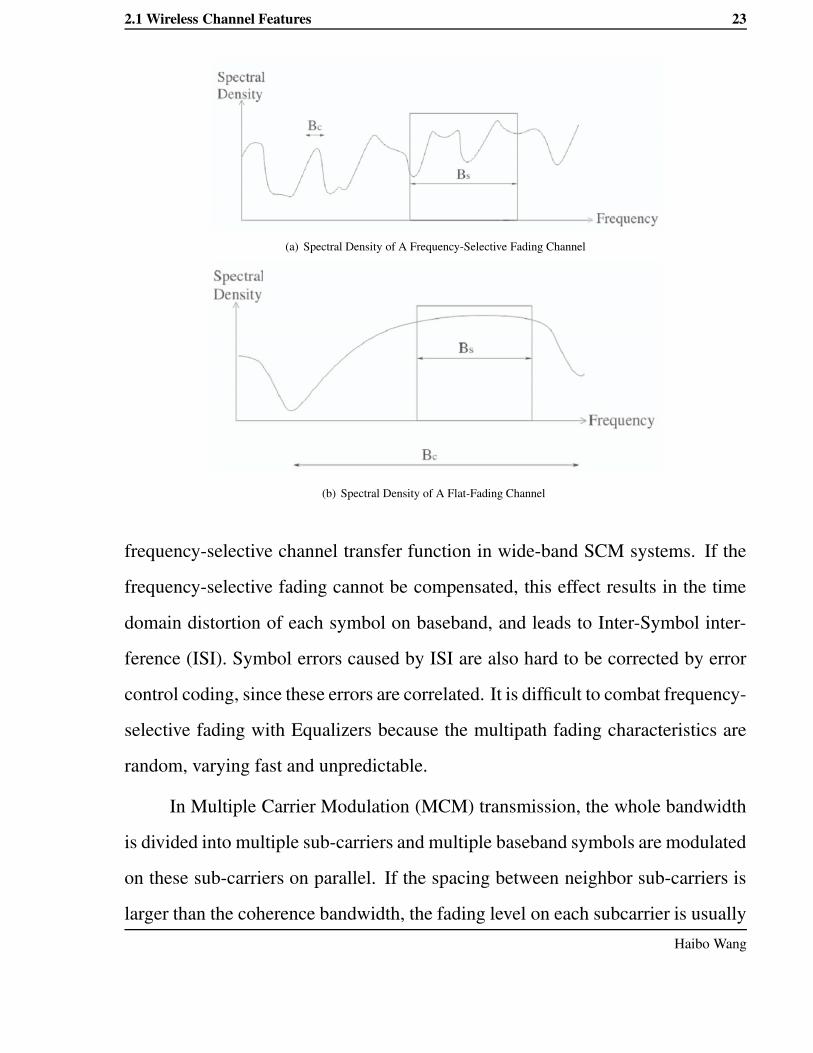
The channel transfer function is the Fourier transform of the impulse re-
sponse, in which the amplitude or power spectrum changes as frequency varies
[3], as depicted in Fig. 2.2(b) and 2.2(a). How quickly the channel changes in
frequency can be measured with frequency coherence, namely coherence band-
width, Bc. This parameter is defined as the smallest value of frequency difference
∆f for which the frequency correlation function equals some suitable correlation
coefficient, e.g. 0.5 or 0.9.
Bc ∝1
Td(2.3)
Coherence bandwidth is inversely proportional to delay spread, and the exact map-
ping between them depends on the correlation coefficient. Therefore, if Bs Bc
as illustrated in Fig. 2.2(a), this channel is a frequency selective channel, whereas
if Bs Bc as illustrated in Fig. 2.2(b), this channel is a frequency flat fading
channel.
2.1.3 Channel Fading versus Modulation
Pathloss and shadowing are semi-static phenomena, and the signal attenuation due
to them can be compensated with careful cellular network planning and power
control. But the effect of Multipath fading is much more difficult to cope with.
For wide-band wireless communication systems, multipath fading causes
frequency-selective fading, because the coherence bandwidth of the channel is
always smaller than the whole transmission bandwidth. For Single Carrier Mod-
ulation (SCM) transmission, each baseband data symbol is modulated over the
whole transmission bandwidth, and the symbol duration is very short since the
data rate is high. Complex Equalizers at the receiver are needed to compensate theAalborg Universitet
2.1 Wireless Channel Features 23
(a) Spectral Density of A Frequency-Selective Fading Channel
(b) Spectral Density of A Flat-Fading Channel
frequency-selective channel transfer function in wide-band SCM systems. If the
frequency-selective fading cannot be compensated, this effect results in the time
domain distortion of each symbol on baseband, and leads to Inter-Symbol inter-
ference (ISI). Symbol errors caused by ISI are also hard to be corrected by error
control coding, since these errors are correlated. It is difficult to combat frequency-
selective fading with Equalizers because the multipath fading characteristics are
random, varying fast and unpredictable.
In Multiple Carrier Modulation (MCM) transmission, the whole bandwidth
is divided into multiple sub-carriers and multiple baseband symbols are modulated
on these sub-carriers on parallel. If the spacing between neighbor sub-carriers is
larger than the coherence bandwidth, the fading level on each subcarrier is usuallyHaibo Wang
24 Chapter 2. Background
flat and the ISI is eliminated. However, the fading level difference still exists
among different sub-carriers, but it can be exploited by link adaptation schemes,
namely, frequency diversity. If the signal quality on one subcarrier is too poor and
the symbol on this subcarrier cannot be correctly received, it will not effect other
symbols. Besides, such symbol errors are independent and are relatively easy to
be corrected by error control coding schemes such as convolutional codes.
In summary, to combat multipath fading in wide-band wireless communica-
tions, this is one important reason to introduce MCM transmission technique such
as OFDM.
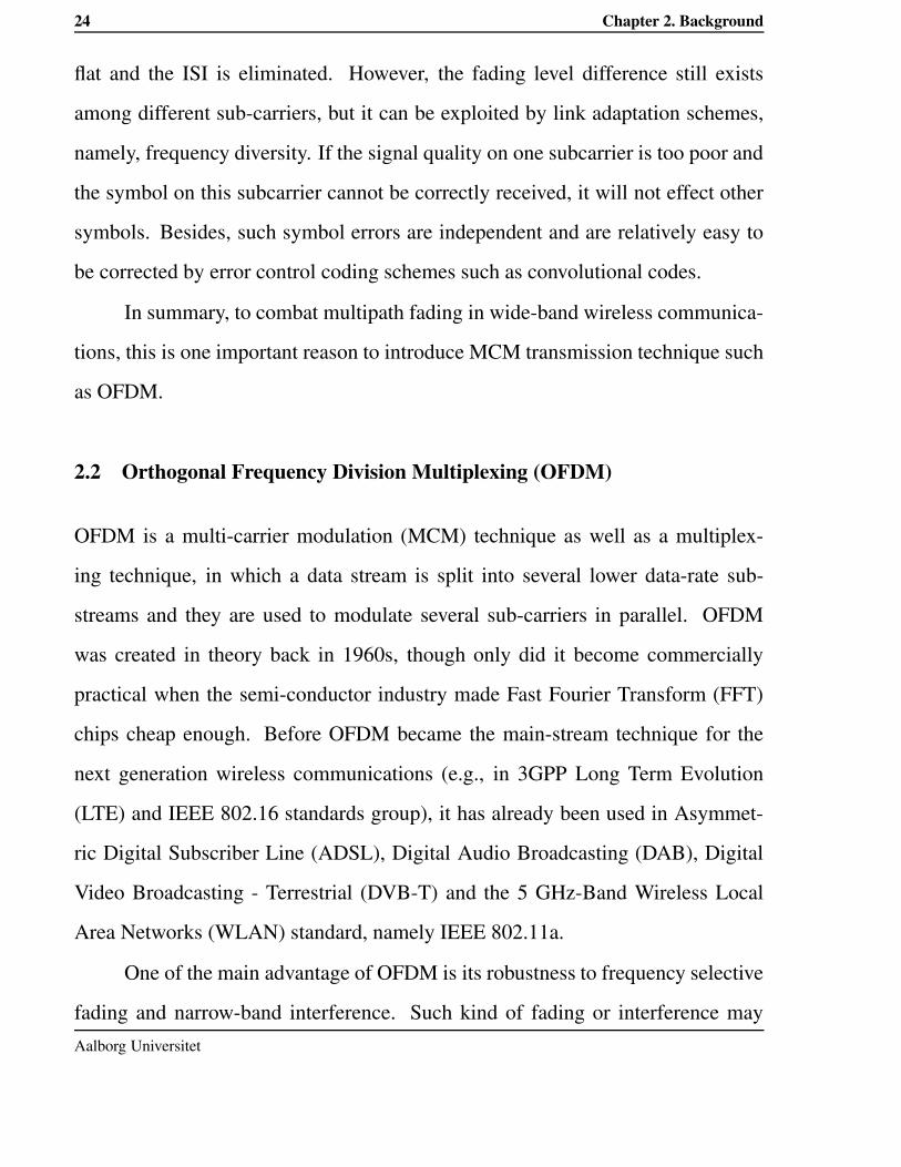
2.2 Orthogonal Frequency Division Multiplexing (OFDM)
OFDM is a multi-carrier modulation (MCM) technique as well as a multiplex-
ing technique, in which a data stream is split into several lower data-rate sub-
streams and they are used to modulate several sub-carriers in parallel. OFDM
was created in theory back in 1960s, though only did it become commercially
practical when the semi-conductor industry made Fast Fourier Transform (FFT)
chips cheap enough. Before OFDM became the main-stream technique for the
next generation wireless communications (e.g., in 3GPP Long Term Evolution
(LTE) and IEEE 802.16 standards group), it has already been used in Asymmet-
ric Digital Subscriber Line (ADSL), Digital Audio Broadcasting (DAB), Digital
Video Broadcasting - Terrestrial (DVB-T) and the 5 GHz-Band Wireless Local
Area Networks (WLAN) standard, namely IEEE 802.11a.
One of the main advantage of OFDM is its robustness to frequency selective
fading and narrow-band interference. Such kind of fading or interference mayAalborg Universitet

2.2 Orthogonal Frequency Division Multiplexing (OFDM) 25
Frequency
8 Sub-carriers
Figure 2.2: OFDM with 8 Sub-Carriers
corrupt an entire SCM link, but it can only affect a small portion of sub-carriers of
a MCM link [1]. Due to this reason, a complex and expensive equalizer is needed
in SCM receivers to compensate the channel transfer function, while in a MCM
system like OFDM, no or only a very simple equalizer is needed.
OFDM is different comparing to FDM in its frequency sub-bands are over-
lapping to achieve the maximum spectrum efficiency, as shown in Fig. 2.2. By
carefully selecting symbol rate and via DFT/IDFT implementation, the inter-subcarrier
interference can be perfectly removed though the sub-carriers are actually over-
lapping, which is the so-called orthogonality. The main features of OFDM can be
concluded as follow:
• Robustness again frequency selective fading and narrow-band interference.
• Maximum spectral efficiency due to no guard bands and the sub-carrier over-
lapping.
• Orthogonality among sub-carriers.
• Eliminate the inter-symbol interference by inserting a cyclic prefix into each
symbol period.Haibo Wang

26 Chapter 2. Background
• Easy and cheap implementation with FFT/IFFT and no or only simple chan-
nel equalizer needed.
• Sensitive to time-frequency synchronization to keep the orthogonality, such
as sub-carrier synchronization.
• Sensitive to non-linear amplification.
The strict mathematical deduction and more detailed explanation of these listed
OFDM features can be found in [1], [7] and [3].
Rec
eive
r
Tran
smitt
er
Pilot symbolinsertion
Binary Data
Serial to parallel
IFFT
InsertCyclic Prefix
DAC
RF
Error Control Coding andInterleaving
Symbol Mapping(Data Modulation)
Complex constellations
Channel estimationfrom Pilot symbol
Binary Data
Parallel to serial
FFT
RemoveCyclic Prefix
ADC
RF
Error control decoding and
de-interleaving
SymbolDe-mapping
Radio Channel
Figure 2.3: An OFDM Transceiver Diagram
A complete OFDM transceiver system diagram is depicted in Fig. 2.3. OnAalborg Universitet

2.2 Orthogonal Frequency Division Multiplexing (OFDM) 27
the transmitter side, binary data is input and Forward Error Correction (FEC) cod-
ing and interleaving are added to protect the data. Interleaving can re-distribute
burst errors introduced by wireless transmission as random errors among original
data, which are easier for FEC decoder to correct than burst errors. Afterwards, a
block of coded bits are assigned to different OFDM sub-carriers (1 bit maps to 1
symbol for Binary Phase Shift Keying (BPSK), 2 bits per symbol for QPSK, 4 for
16 16QAM, etc.) and modulated to different constellation points respectively. At
this stage, the data is mapped into a serial stream of complex numbers. Then pilot
symbols are inserted. The serial symbols are converted to parallel form and the
Inverse Fast Fourier Transform (IFFT) operation is applied. A Cyclic prefix [1] is
inserted in every data symbol according to the system specification, and the data
is now in serial form (time domain) again . So far the baseband OFDM modula-
tion has been completed, and a Digital to Analogue Converter (DAC) is applied
to transform the digital symbols to analog signal. Finally Radio Frequency (RF)
modulation is performed to up-convert the signals onto the carrier frequency.
After the transmitted OFDM signal has gone through the wireless channel,
the signal is captured by the receiver antenna and downconverted to baseband,
and further converted to digital domain with Analog-to-Digital Converter (ADC).
FFT is then performed to demodulate the OFDM signal, and the parallel symbols
are mapped back to serial. At this point, channel estimation can be fulfilled with
the demodulated pilots. The estimations helps detecting the data from the signal
constellation points. At the end, FEC decoding and de-interleaving are performed
to recover the originally bit stream.
Haibo Wang

28 Chapter 2. Background
2.2.1 OFDMA
A fraction of OFDM sub-carriers can be grouped to make up a sub-channel, and
different sub-channels can be allocated to different users to construct the multiple
access technique, namely OFDMA. At the beginning it was proposed for Cable
Television (CATV) systems [5], and later for wireless communications [6].
The simplest OFDMA channel resource allocation scheme is to assign sub-
channels to users in a static way as depicted in Fig. 2.4. In this scheme, the sub-
channel assignment stays the same for the user during a whole connection, or
at least for a considerable time period, i.e., during a service session. However,
u1
u2
u3
u4
u1
u2
u3
u4
u1
u2
u3
u4
u1
u2
u3
u4
TS1 TS2 TS3 TS4 t
f
f4
f3
f2
f1
Figure 2.4: OFDMA with Static FDMA Scheme
such a static Frequency Division Multiple Access (FDMA) scheme is not efficient
when a specific user is in deep fading channel. Actually sub-channels and Time-
Slots (TS) can both be dynamically allocated to users according to their channel
conditions and data rate requirements as shown in Fig. 2.5. Theoretically it has
been proved that if the instantaneous channel condition on each subcarrier of each
user is available, optimal allocation for subcarrier, time-slot and power in eachAalborg Universitet

2.2 Orthogonal Frequency Division Multiplexing (OFDM) 29
subcarrier will be possible to fully utilize user-diversity and to achieve the best
system performance (i.e., maximum cell throughput, low BER) [8].
u1
u1
u2
u2
u1
u3
u2
u2
u1
u3
u3
u4
u2
u2
u3
u4
TS1 TS2 TS3 TS4 t
f
f4
f3
f2
f1
Figure 2.5: OFDMA with Fully Dynamic Frequency-Time Block Allocation
There are also two methods to construct sub-channels, the adjacent mode
and the distributed mode [7], depending on whether the sub-carriers in a sub-
channel are adjacent to each other or distributed among the whole transmission
bandwidth with a certain frequency interval [9]. As illustrated in Fig. 2.6, the
sub-carriers of a sub-channel in adjacent mode are contiguous, and the channel
conditions of them may be similar. In this case one pilot sub-carrier can be used
to detect the channel condition of the whole sub-channel, which may reduce the
channel information feedback needed by AMC in the transmitter side. Also one
modulation and coding combination can be applied to one sub-channel. Both of
these advantages reduce the implementation complexity of sub-channel allocation
and AMC. However, channel fading will also degrade the throughput of an adja-
cent sub-channel seriously, since one fading ditch in the channel transfer function
curve (see Fig. 2.2(a)) can effect on several sub-carriers. In the distributed mode,Haibo Wang

30 Chapter 2. Background
Subcarriers
SubChannel1
SubChannel2
SubChannel3
SubChannel4
Subcarriers
SubChannel1
Subcarrier ofSubchannel 1
Subcarrier ofSubchannel 2
Subcarrier ofSubchannel 3
Subcarrier ofSubchannel 4
Subcarrier ofSubchannel 5
Adjacent Mode
Distributed mode
Figure 2.6: OFDMA Sub-Channel Modes
the sub-carriers are much further apart to each other, so they are more independent
and more robust against frequency-selective fading, especially under harsh chan-
nel environment (i.e., when users are with high mobility). This is called channel
diversity gain. On the other hand, it would be complex to make channel allocation
and hard to implement AMC in distributed mode.
2.2.2 OFDMA-Based Standards Groups
There are two main next generation mobile OFDMA standards groups, the IEEE
802.16e (or the so-called WiMAX) and the 3GPP UMTS-LTE. They basically
selected very similar specifications on the physical (PHY) layer, e.g., both of them
support scalable channel bandwidth, AMC, MIMO techniques. Their differenceAalborg Universitet
2.2 Orthogonal Frequency Division Multiplexing (OFDM) 31
is that WiMAX is a group trying to include different stands covering from fixed
wireless Internet access network to cellular-like mobile networks, while 3GPP
LTE is a evolution from the pure mobile cellular system, UMTS.
2.2.2.1 IEEE 802.16 Standards Group
The IEEE 802.16 standards group is also called Worldwide Inter-operability for
Microwave Access (WiMAX). This standardization group is proposed to provide
wireless data in a variety of ways, from fixed point-to-point links to full mobile
cellular type access. In this group, the amendment 802.16e-2005 (often referred to
in shortened form as 802.16e) is called Mobile WiMAX since it covers full mobility
support and promises to provide high data rate service anytime, anywhere [10].
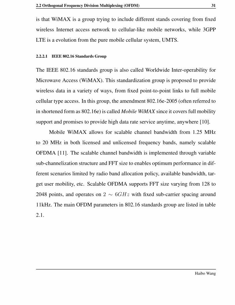
Mobile WiMAX allows for scalable channel bandwidth from 1.25 MHz
to 20 MHz in both licensed and unlicensed frequency bands, namely scalable
OFDMA [11]. The scalable channel bandwidth is implemented through variable
sub-channelization structure and FFT size to enables optimum performance in dif-
ferent scenarios limited by radio band allocation policy, available bandwidth, tar-
get user mobility, etc. Scalable OFDMA supports FFT size varying from 128 to
2048 points, and operates on 2 ∼ 6GHz with fixed sub-carrier spacing around
11kHz. The main OFDM parameters in 802.16 standards group are listed in table
2.1.
Haibo Wang

32 Chapter 2. Background
Parameter Mobile WiMAX ScalableOFDMA-PHY
FFT size 128 512 1024 2048Number of used data subcarriers 72 360 720 1440Number of pilot subcarriers 12 60 120 240Number of null subcarriers 44 92 184 368Cyclic prefix (Tg/Tb) 1/32, 1/16, 1/8, 1/4Channel bandwidth (MHz) 1.25 5 10 20Subcarrier frequency spacing (kHz) 10.94Useful symbol time (µs) 91.4Guard time assuming 12.5 % (µs) 11.4OFDM symbol duration (µs) 102.9Number of OFDM symbol in 20ms frame (µs) 198.0
Table 2.1: OFDM Parameters in Mobile WiMAX [11]
2.2.2.2 UMTS-LTE
The 3GPP working groups have developed their radio access network standards
in Universal Terrestrial Radio Access Network (UTRAN) from Wideband Code
Division Multiple Access (WCDMA) to High-Speed Downlink Packet Access
(HSDPA) and High-Speed Uplink Packet Access (HSUPA), all based on single
carrier CDMA technique. OFDMA has been proposed for the long term evolution
of UTRAN (called Evolved UTRAN (EUTRAN)) as downlink multiple access
technique, while Single-Carrier FDMA (SC-FDMA) will be adopted for uplink
[12, 13]. LTE feasibility study has been finalized on September 2006 , after which
actual specification development would be fulfilled.
The DL OFDMA in LTE also supports scalable bandwidth from 1.25 to
20MHz, with fixed sub-carrier spacing 15kHz. LTE fully exploits advanced tech-
niques like Layer 1 Hybrid Automatic Repeat request (L1 HARQ), frequency do-
main scheduling, MIMO antenna technologies and AMC [12, 13]. Comparing toAalborg Universitet

2.3 Radio Resource Management (RRM) 33
UTRAN, EUTRAN has more functionalities on Node B and shortens the Trans-
mission Time Interval (TTI) even to 0.5 ms (TTI is 2 ms in HSDPA). With the
help of such short TTI and fast L1 ARQ, the round-trip delay can be reduced to 5
ms. More detailed LTE specifications can be found in the 3GPP website.
2.3 Radio Resource Management (RRM)
As introduced in the first chapter, RRM approaches are investigated for wireless
multicast in this PhD project. This section discusses the available degrees of free-
dom in multicast scenarios as well as some OFDM specific issues.
The dominant cost for deploying a wireless network is normally the base sta-
tions (real estate costs, planning, maintenance, distribution network, energy, etc),
and sometimes frequency license fees is also highly expensive. Therefor the typi-
cal objective of RRM is to maximize the system spectral efficiency in bit/s/Hz (or
Erlang/MHz) per base station, with a certain level of QoS constraints. The con-
straints involve BER, packet loss rate or outage rate (as well as other metrics like
delay, jitter, etc) due to noise, attenuation caused by long distances, fading caused
by shadowing and multipath fading, co-channel interference and other forms of
distortion. The QoS is also affected by blocking due to admission control, schedul-
ing starvation or unable to the guarantee quality of service class that is requested
by the users.
In general, RRM optimization problem can be formulated as either min-
imizing a cost metric (e.g. transmit power) or maximizing a reward metric (e.g.
throughput) under system hardware constraints, service specific QoS requirements
and the overall system state (e.g, the channel fading states of all the receiversHaibo Wang

34 Chapter 2. Background
within a cell). In this thesis, our target is to maximize performance metric under
QoS constraints.
Though RRM covers a wide range of approaches, in the scenario delimited
in chapter 1 we are mainly interested in the link adaptation methods, namely AMC,
power control and ARQ for our multicast problems. Admission control, handover
and scheduling among different users/services are out of the scope of our work.
2.3.1 AMC and Power Adaptation
The term power control was frequently used to refer to the process of varying
transmitting power level in order to keep a stable SINR target for voice service
(with fixed transmission data rates) like in GSM and WCDMA, or in order to
suppress interferences. However in the context of performance optimization for
multimedia services, power is adjusted according to the channel condition rather to
provide high data rate. Hence the term ’power adaptation’ is employed instead of
’power control’ from now on. Varying modulation rate and coding rate, no matter
separately or jointly, change the transmitted data rate. So AMC (or just Adaptive
Modulation or Adaptive Coding alone) can also be called data rate adaptation.
AMC and power adaptation pro-actively adjusts the transmitting data rate
and power to adapt to the estimated channel conditions. If the estimated channel
conditions are accurate, theoretically they can exploit the channel capacity in every
transmission burst. The price is that the overhead in feedback channels to report
channel conditions could be large. It has been proved in [15] that the Shannon ca-
pacity of a flat-fading channel can either be achieved by varying both transmission
rate and power, or be achieved by varying the transmit power alone [16]. More-Aalborg Universitet

2.3 Radio Resource Management (RRM) 35
over, it has also been revealed in [15] that varying both power and rate leads to
a negligible capacity gain over varying the rate alone. Similar conclusions were
drawn for achievable data rates in [17, 18].
2.3.2 Water-Filling Principle
In this subsection we discuss the possible dynamic schemes specific in OFDM
for multicast radio channel. The available radio resources that can be manipu-
lated include transmit power, modulation and coding allocation schemes, subcar-
rier or subchannel allocation. The dynamic utilizing of resources can exploit the
frequency-selective nature of wireless channels due to Multipath fading. Usually
the sub-carrier spacing of OFDM systems is larger than the channel coherence
bandwidth, hence the attenuation within each sub-carrier is flat and the fading
level of different sub-carrier is independent to each other.
For a time interval smaller than the channel coherence time of a wide-band
wireless channel, the fading level on each sub-carrier stay constant, while the level
among different sub-carriers are identical independent distributed (i.i.d) due to the
frequency-selective nature of the channel. The optimal power allocation scheme
on OFDM sub-carriers to maximize the channel capacity is given by the "water-
filling" theorem [19] based on information theory, as illustrated in Fig. 2.7. This
theorem states, when the total transmit power is fixed, more power should be as-
signed to the frequency areas with less attenuation (better channel condition), until
the sum of assigned power and the reciprocal of channel gain per frequency is aHaibo Wang

36 Chapter 2. Background
1/G(f)
f
Water level
Channel Bandwidth
P(f)
Figure 2.7: Illustration of "Water-Filling" Solution
constant over the whole bandwidth. Such as:
S(f) +1
G(f)= constant (2.4)
where S(f) is the power function along frequency, G(f) is the channel gain func-
tion along frequency.
The water-filling solution is not directly implementable for two reasons.
First the OFDM sub-carriers are discrete rather than continuous as in the water-
filling solution; secondly, there is not a directly continuous mapping between
power and bits per second in practice. The feasible data rate are a discrete set
of numbers achieved by different combinations of modulation and error control
coding schemes. Besides, any practical modulation has a certain “gap” between
its achievable bits per second and the Shannon capacity. These issues will be dis-
cussed further in the following chapters.
The water-filling principle can be implemented in some discrete version of
it, in terms of bit- or power-loading algorithms. In the optimal form the number ofAalborg Universitet

2.3 Radio Resource Management (RRM) 37
bits transmitted per sub-carrier and the power assigned on each sub-carrier should
be jointly allocated. But either bit- or power-loading can be implemented alone to
achieve a certain sub-optimal performance for simplicity. Therefor, all these bit-
and/or power-loading algorithms are referred to as adaptive loading algorithms in
further discussion.
The joint power and rate allocation in water-filling form may apply not only
along frequency dimension, but also along the channel gain distribution and more
dimensions. How this form could be adopted in multicast channel is to be studied
in the rest of this thesis.
2.3.3 ARQ
ARQ schemes can be divided into the following categories :
• Plain ARQ
Well-know plain ARQ schemes include Stop-And-Wait (SAW), Go-Back-N
(GBN), and Selective Retransmission (SR), and more details can be found in
International Engineering Task Force (IETF) Request for Comments (RFC)
3366 and [23].
– SAW ARQ
In SAW ARQ, a sender sends one data packet, and then waits. The re-
ceiver sends an Acknowledgement (ACK) once receiving a correct packet.
The sender will only send the next packet once it receives the ACK for
the first packet within a certain time. If the ACK has not come in time,
known as a timeout, the sender sends the first packet again. In SAW, the
fact that the sender needs to wait for every ACK wastes its transmissionHaibo Wang

38 Chapter 2. Background
capacity during the waiting time.
– GBN ARQ
GBN is more efficient than SAW in that it allows the sender continue
sending a number of packets limited by a sliding window without receiv-
ing an ACK. The GBN ARQ receiver keeps tracking the received packet
sequence numbers, and if one packet is incorrect, it will reject the follow-
ing packets even if they are correct. The sender, after sending all packets
in its window, will have to go back to the last ACK and restart send-
ing from the first lost packet. In this protocol, some packets could have
been correctly accepted by the receiver but may be rejected only because
they follow an incorrect packet, and are to be resend, which also wastes
transmission capacity.
– SR ARQ
Unlike GBN, SR ARQ allows the receiver to accept packets until the
sender has emptied its window, and the sender needs only to resend the
lost packets identified by ACKs/NACKs. Hence SR ARQ is more effi-
cient than GBN.
• Hybrid-ARQ (HARQ)
Hybrid-ARQ combines ARQ and Forward-Error-Correction coding (FEC).
There exist three types of HARQ: Type I, Type II and Type III, where Type
III HARQ can be seen as a variation of Type II HARQ.
– Type I HARQ
In Type I HARQ, the original information and Error Detection (ED) par-
ity bits are further encoded by a FEC encoder (such as a Turbo coder)Aalborg Universitet
2.3 Radio Resource Management (RRM) 39
[35, 45] and sent to the receiver; if the receiver fails to decode this data
block correctly, the same data block will be send again as in a pure ARQ.
The receiver can either discard the first block or store it to combine with
the retransmitted block, which is called Chase Combining (CC) in UMTS
HSDPA [45]. Here FEC and ARQ are operated separately, or so-called
Layered FEC-ARQ [26].
– Type II HARQ and Type III HARQ
In Type II HARQ, multiple parity code blocks are created for the original
information, with Incremental Redundancy (IR)/reliability as the num-
ber of parity blocks increase. Only the original information and the least
parity blocks are sent in the first transmission, and more parity blocks
will only be sent as the receivers request [35, 45]. If each retransmis-
sion packet can be decoded independently, such HARQ is called Type III
HARQ.
The performance of each of these ARQ protocols in uncash channels has been
studied systematically. Plain ARQ (SAW and SR), Type I and Type II HARQ in
uncash mobile link was analyzed in [35]. It revealed that pure ARQ achieves the
best throughput efficiency under good channel condition, but degrades the most
as channel condition get worse; Type I HARQ performs better in poor channel
condition while lost efficiency in good channel; Type II HARQ with SR performs
the best in both cases. It is proved in [45] that IR (Type II HARQ) is slightly
more efficient in throughput than CC (Type I HARQ) in a very detailed HSDPA
simulation environment, but the difference is very small or even diminishes as the
link adaptation error decreases.Haibo Wang

40 Chapter 2. Background
Also there are many existing works on the ARQ performance study for
multicast links. The performance of plain ARQ schemes have been investigated
in [31, 32, 33, 34], which confirmed that SAW is the most inefficient in terms of
throughput [33], and SR is more efficient than GBN [33, 34]. Multicast HARQ
schemes based on Reed-Solomon codes (namely Maximum Distance Separable
(MDS) code) are analyzed for satellite links in [36]. The authors of [37] fur-
ther utilized Generalized Minimum Distance (GMD) decoding for MDS, which
improved the throughput a bit but increased the decoding complexity and delay.
Three HARQ schemes based on packet level Reed-Solomon codes were designed
in [5] for UMTS downlink multicast channel, and the authors pointed out which
design is better would rather depend on the multicast channel error process in real-
ity (e.g, independent error model or burst error model). The authors of [6] further
proposed two more HARQ schemes as the extensions of scheme A2 and A3 in [5]
and achieved a certain improvement in throughput and mean Service Data Unit
delay, especially when the Multicast group size is large. However, the scalability
of multicast ARQ protocols remains a problem [2].
2.4 State-of-the-art
In this section we discuss how the link adaptation approaches introduced in Sec. 2.3
can be adopted in multi-user systems, as well as the related works.
2.4.1 OFDM link adaptation and multi-user diversity
LA assigns modulation, coding, transmit power, and/or other signal transmission
parameters according to the instantaneous channel condition, in order to increaseAalborg Universitet

2.4 State-of-the-art 41
the spectrum efficiency and reliability of wireless systems. The water-filling prin-
ciple introduced in Sec. 2.3.2 reveals, for an OFDM system with power con-
straint, the system spectral efficiency is maximized by transmitting with higher
data rate (higher modulation constellation and less coding protection) and more
power when the channel condition is good, while transmitting with lower date rate
and less power when the channel condition is bad.
Different users in a wireless system experience different and independent
channel attenuations and noise/intereferences, which can be exploited as multi-
user diversity. It is quite unlikely that a user is in deep fading on all the subcarriers,
or all users are in deep fading on the same subcarrier. Hence the time-subcarrier
can be dynamically assigned to different users according to their instantaneous
channel conditions on different subcarriers to improve the spectral efficiency, as
illustrated in Fig. 2.5, such dynamic approach is also called scheduling.
2.4.2 Related work with multiple unicast users
Based on water-filling principle and multi-user diversity, joint allocate/adapt sub-
carrier and data rate to multiple users was first proposed by Wong [8], target at
minimizing total transmitting power with data rate and BER constraints. Similar
dynamic allocation and adaptation work was done in [47], but the optimization
target is to maximize data rate with power and BER constraints. However, the
computational complexity of Wong’s algorithm [8] is very high, and several more
practical algorithms are proposed in [48].
Scheduling can maximize the system spectral efficiency, but it may also have
the users in bad channel conditions experiencing high delay and low data rate.Haibo Wang

42 Chapter 2. Background
Proportional Fair Scheduling (PFS) is designed to allowing all users a minimal
level of QoS by assigning each data flow a scheduling priority which is inversely
proportional to its anticipated resource consumption [50]. PFS can be tailored to
integrate different QoS classes and achieve a high average user satisfaction [50].
On the other hand, joint time-subcarrier scheduling with PFS in OFDM system is a
prohibitively complex problem. The authors of [51] derived the upper bounds for
optimal PFS with convex optimization, and proposed sub-optimal solutions with
much lower complexity comparing to the optimal one.
2.4.3 Related work with one multicast group
With one group of multicast users sharing a common downlink channel, schedul-
ing is not an option any longer and link adaptation and ARQ remains the main
dynamic adaptation approaches. An iterative optimization algorithm using link
adaptation was proposed to minimize the total error ratio of all users under power
and data constraints in OFDM [52]. In [53], based on a dominant SNR-based LA
scheme, the authors appropriately discarded some inefficient transmission modes
to convert the goodput-maximization problem to a concave optimization prob-
lem, and derive the optimal adaptation power and AMC modes correspondingly.
However, in this approach, only the goodput is considered but there is no error
constraints included.
2.5 Summary
This chapter presents the channel features and OFDM transmission technique re-
lated to our wireless cellular scenario, as well as available link adaptation tech-Aalborg Universitet

2.5 Summary 43
niques for the multicast channel. For the concerned wide-band wireless system,
multipath fading is the most difficult fading issue to cope with, and OFDM can
help to split the whole frequency-selective fading channel into a set of frequency-
flat fading channels over each subcarrier, where different LA (e.g., AMC, power
adaptation, ARQ) can be adopted to improve wireless multicast performance.
Haibo Wang

Bibliography
[1] Shinsuke Hara and Ramjee Prasad, Multicarrier Techniques for 4G Mobile
communications, pp. 27-39, Artech House, 2003.
[2] G. L. Stüber, Principles of Mobile Communication, 2nd ed., Kluwer Aca-
demic Publishers, 2001.
[3] D. Tse and P. Viswanath, Fundamentals of Wireless Communications, Cam-
bridge University Press, 2005.
[4] M. I. Rahman, Channelization, Link Adaptation and Multi-antenna Tech-
niques for OFDM(A) Based Wireless Systems, PhD thesis, Sept. 2007.
[5] H. Sari, Y. Levy and G. Karam, “Orthogonal Frequency-Division Multiple
Access for the Return Channel on CATV Networks,” in Proc. IEEE ICT’96,
Istanbul, April 1996.
[6] H. Sari, Y. Levy and G. Karam, “An Analysis of Orthogonal Frequency-
Division Multiple Access,” in Proc. IEEE GLOBECOM’97, vol. 3, pp. 1635-
1639, Nov. 1997.44

BIBLIOGRAPHY 45
[7] H. Yaghoobi, “Scalable OFDMA Physical Layer in IEEE 802.16 Wireless
MAN,” in Intel Technical Journal, vol. 8, no. 3, pp. 201-212, 2004.
[8] C. Y. Wong, R. S. Cheng, K. Letaief, and R. Murch, “Multiuser OFDM with
adaptive subcarrier, bit and power allocation,” in IEEE J. Select. Areas Com-
mun., vol. 17, no. 10, pp. 1747-1758, Oct. 1999.
[9] D. Galda and H. Rohling, “A Low Complexity Transmitter Structure for
OFDM-FDMA Uplink Systems,” in IEEE VTC’02 Spring, Birmingham,
USA, May 2002.
[10] The IEEE 802.16 Working Group on Broadband Wireless Access Standards,
“Part 16: Air Interface for Fixed and Mobile BraodbandWireless Access Sys-
tems,” in Tech. Rep., IEEE P802.16e Standard Document, Dec. 2005.
[11] Z. Abichar, Y. Peng and J. M. Chang, “WiMAX: The Emergence of Wireless
Broadband,” in IEEE IT Magazine, vol. 8, no. 4, pp. 44 − 48, Jul. 2006.
[12] 3GPP Technical Report, “Physical layer aspects for evolved Universal Ter-
restrial Radio Access (UTRA), release 7,” TR 25.814, v7.0.0, Jun. 2006.
[13] A. Toskala, H. Holma, K. Pajukoski and E. Tiirola, “UTRAN Long Term
Evolution in 3GPP,” in proc. IEEE PIMRC’06, Helsinki, Finland, Sept. 2006.
[14] J. Zander, “Radio Resource Management in Future Wireless Net works : Re-
quirements and Limitations,” in IEEE Commun. Magazine, pp. 30-36, Aug.
1997.
[15] A. J. Goldsmith and P. Varaiya, “Capacity of fading channels with channelHaibo Wang

46 BIBLIOGRAPHY
side information,” in IEEE Trans. Inform. Theory, vol. 43, pp 86-92, Nov.
1997.
[16] G. Caire and S. Shamai, “On the capacity of some channels with channel
state information,” in IEEE Trans. Inform. Theory, vol. 45, pp 2007-2019,
Sept. 1999.
[17] A. J. Goldsmith and S. Chua, “Variable-rate variable-power MQAM for fad-
ing channels,” in IEEE Trans. Commun., vol. 45, pp. 1218−1230, Oct. 1997.
[18] Seong Taek Chung, Andrea J. Goldsmith, “Degrees of Freedom in Adaptive
Modulation: A Unified View,” in IEEE Trans. Commun, vol. 49, no. 9, pp
1561-1571, Sept. 2001.
[19] C. E. Shannon, “Communication in the presence of noise,” in Proc. IRE, vol.
37, pp. 10-21, Jan. 1949.
[20] M. Ergen, S. Coleri, and P. Varaiya, SQoS aware adaptive resource alloca-
tion techniques. for fair scheduling in OFDMA based broadband wireless
systems,” in IEEE Trans. Broadcasting, vol. 49, no. 4, December 2003.
[21] H. Yin and H. Liu, “An efficient multiuser loading algorithm for OFDM
based broadband wireless systems,” IEEE Globecom, 2000.
[22] C. Zhou, G. Wunder, and T. Michel, “Utility Maximization for OFDMA sys-
tems over discrete sets,” in Proc. IEEE Int. Conf. on Communications (ICC),
Glasgow, June 2007.
[23] A. S. Tanenbaum, Computer Networks, 4th ed., pp. 200-223, Person Educa-
tion International, 2003.Aalborg Universitet

BIBLIOGRAPHY 47
[24] P. Larsson and N. Johansson, “Multi-User ARQ,” Proc. of IEEE VTC’06-
Spring, Melbourne, Australia, May 2006.
[25] J. W. Atwood, “A classification of reliable multicast protocols,” IEEE
Nextwork, vol. 18, no. 3, pp. 24-34, May-June 2004.
[26] J. Nonnenmacher; E. W. Biersack, and D. Towsley, “Parity-based loss re-
covery for reliable multicast transmission,” Networking, IEEE/ACM Trans-
actions on, vol. 6, no. 4, pp. 349-361, Aug. 1998.
[27] L. H. Lehman, S. J. Garland, D. L. Tennenhouse, “Active reliable multicast,”
Proc. IEEE INFOCOM’98, vol 2, pp. 581-589, 29 March-2 April, 1998.
[28] P. Radoslavov, C. Papadopoulos, R. Govindan, D. Estrin,“A comparison of
application-level and router-assisted hierarchical schemes for reliable multi-
cast,” Networking, IEEE/ACM Trans., vol 12, no 3, pp. 469 482, June 2004.
[29] E. R. Berkekamp, Algebraic Coding Theory, McGrawHill, 1968.
[30] F. J. MacWilliams and N. J. A. Sloane, The Theory of Error Correcting
Codes, North-Holland, 1977.
[31] S. B. Calo and M. C. Easton, “A broadcast protocol for file transfer to multi-
ple sites,” IEEE Trans. Commun., vol. 29, no. 11, pp. 1701-1707, Nov. 1981.
[32] K. Mase, T. Takenaka, H. Yamamoto, and M. Shinohara, “Go-back-N ARQ
schemes for point-to-multipoint satellite communications,” IEEE Trans.
Commun., vol. 31, no. 4, pp. 583-589, Apr. 1983.
[33] I. S. Gopal and J. M. Jaffe, “Point-to-multipoint communication over broad-
cast links,” IEEE Trans. Commun., vol. 32, no. 9, pp. 1034-1044, Sept. 1984.Haibo Wang

48 BIBLIOGRAPHY
[34] K. Sabnani and M. Schwartz, “Multidestination protocols for satellite broad-
cast channels,” IEEE Trans. Commun., vol. 33, no. 3, pp. 232-240,
Mar. 1985.
[35] R. Comroe, D. Costello, “ARQ Schemes for Data Transmission in Mobile
Radio Systems”, IEEE Selected Areas in Commun., vol. 2, no. 4, pp. 472-
481, July 1984.
[36] J. J. Metzner, “An improved broadcast retransmission protocol,” IEEE Trans.
Commun., vol. 32, no. 6, pp. 679-683, Jun. 1984.
[37] K. Sakakibara, M. Kasahara, “A multicast hybrid ARQ scheme using MDS
codes and GMD decoding,” IEEE Trans. Commun., vol. 43, no. 12, pp. 2933-
2940, Dec. 1995.
[38] L. Andrey, V. Vladimir, and Y. Mikhail, “Multicast QoS Support in IEEE
802.11 WLANs,” IEEE MASS’07, Oct. 2007.
[39] J. Y. Lim, T. M. Chung, “Enhanced token delivery scheme for reliable
multicasting in wireless networks,” In Proc. IEEE PRIS’01, pp. 214-217,
Dec. 2001.
[40] F. Fitzek, M. Rossi, and M. Zorzi, “Error Control Techniques for Efficient
Multicast Streaming in UMTS Networks,” in Proc. SCI 2003, 2003.
[41] G. D. Papadopoulos, G. Koltsidas, and F. N. Pavlidou, “Two Hybrid ARQ Al-
gorithms for Reliable Multicast Communications in UMTS Networks,” IEEE
Commun. Letters, vol. 10, no. 4, pp. 260-262, Apr. 2006.Aalborg Universitet

BIBLIOGRAPHY 49
[42] Y. Yamauchi, “On the packet radio multicast scheme for the personal com-
munications era,” in Proc. IEEE ICCS’94, vol. 2, pp. 576-580, Singapore,
Nov. 1994.
[43] M. Chipeta, M. Karaliopoulos, B. G. Evans and R. Tafazolli, “On the use of
packet-level FEC and data carousels for the delivery of broadcast/multicast
services to mobile terminals,” IEEE VTC ’05-Spring, Stockholm, Sweden,
May 2005.
[44] Q. Zhang; F. Fitzek; V. B. Iversen, “Design and Performance Evaluation of
Cooperative Retransmission Scheme for Reliable Multicast Services in Cel-
lular Controlled P2P Networks,” IEEE PIMRC 2007, Athens, Greece, Sept.
2007.
[45] F. Frederiksen and T. E. Kolding, “Performance and Modeling of
WCDMA/HSDPA Transmission/H-ARQ Schemes,” In Proc. IEEE VTC’02-
Fall, Vancouver, Canada, Sept. 2002.
[46] S. Sesia, G. Caire, and G. Vivier, “On the Scalability of H-ARQ Systems in
Wireless Multicast,” in Proc. IEEE ISIT’04, pp. 321-321, 2004.
[47] Y. J. Zhang and K. B. Letaief, “Multiuser Adaptive Subcarrier- and-Bit Allo-
cation with Adaptive Cell Selection for OFDM Systems,” IEEE Trans. Wire-
less Commun., vol. 3, no. 5, pp. 1566, Sept. 2004.
[48] G. Song and Y. Li, “Cross-Layer Optimization for OFDM Wireless Networks
Part II: Algorithm Development,” IEEE Trans. Wireless Commun., vol. 4, no.
2, pp. 625 ∼ 634, Mar. 2005.Haibo Wang

50 BIBLIOGRAPHY
[49] H. J. Kushner and P.A. Whiting, “Convergence of proportional-fair sharing
algorithms under general conditions,” IEEE Trans. Wireless Commun., vol.
3, no. 4, pp. 1250 ∼ 1259, July 2004.
[50] P. Svedman, S. K. Wilson and B. Ottersten, “A QoS-aware proportional fair
scheduler for opportunistic ,” IEEE Vehicular Technology Conference, 2004.
VTC2004-Fall., 26-29 Sept. 2004.
[51] M. Kaneko, P. Popovski and J. Dahl, “Proportional Fairness in Multi-Carrier
System with Multi-Slot Frames: Upper Bound and User Multiplexing Algo-
rithms,” IEEE Trans. Wireless Commun., vol. 7, no. 1, pp. 22-26, Jan. 2008.
[52] A. Demarez and D. Boulinguez, “Adaptive Bit And Power-Loading For Mul-
ticast OFDM Transmissions In Rayleigh Fading Channels,” International
Symposium on Wireless Communication System, 6-8 Sept. 2006.
[53] Q. Du and X. Zhang, “Joint Power and Constellation Size Adaptation for
Mobile Multicast Employing MQAM Over Wireless Fading Channels,” IEEE
International Conference on Communications (ICC ’07), 24-28 June 2007.
[54] J. Y. Lee, J. Choi, K. Park, and S. Bahk, “Realistic Cell-oriented Adaptive
Admission Control for QoS Support in Wireless Multimedia Networks,” in
IEEE Trans. on Vehicular Tech., 52(3), May 2003.
[55] Q. Liu, S. Zhou, and G. B. Giannakis, “Cross-Layer combining of adap-
tive Modulation and coding with truncated ARQ over wireless links,” IEEE
Trans. Wireless Commun., vol. 3, no. 5, pp. 1746-1755, Sept. 2004.
Aalborg Universitet

Chapter 3
Rate Adaptation for Mobile Multicast
In this chapter we investigate the Adaptive Modulation (AM) strategies for Multi-
cast service in OFDMA systems. To maximize the average throughput for a group
of Multicast users, and keep as many as possible group members having accept-
able QoS during a service session, a Reward function is firstly defined to evaluate
this two-tuple optimization problem. Then a Local Reward strategy is designed
and evaluated together with other AM schemes with a self-developed simulation
tool. Based on the evaluation results, the evaluation metric is improved, and a
history-based BER threshold adaptation is proposed to exploit the throughput-
BER tradeoff further.
The chapter is organized as follows. Sec.3.1 explains the motivation. Sec. 3.2
presents the system model and assumptions. Sec. 3.3 describes our simulation
tool. Sec. 3.4 proposes the first Reward function, corresponding AM schemes and
numerical results, and Sec. 3.5 presents the second Reward function, correspond-
ing AM algorithms and results. Sec. 3.6 summarizes the whole chapter.51
52 Chapter 3. Rate Adaptation for Mobile Multicast
3.1 Motivation
OFDM-based link adaptation techniques (e.g., power allocation, subcarrier alloca-
tion, adaptive modulation and coding) for uncash scenarios have been extensively
studied in [6], [7], [8]. AM has been proved as an effective approach to improve
the system performance if CSIs are provided. For uncash services, OFDM sub-
carriers can be allocated adaptively to different mobile users in downlink based on
their channel quality. This diversity option helps the subchannel of each user avoid
deep fading caused by multipath frequency-selective fading. By using Adaptive
Modulation, high spectral efficiency can be achieved by selecting the highest mod-
ulation rate with a given acceptable BER constraint [8]. However, in the multicast
case if all group members have to share the same downlink subchannel, deep fad-
ing subcarriers cannot be skipped by frequency scheduling. In this case whether
and how the per subcarrier AM can improve efficiency (such as throughput) while
keeping the BER acceptable is a problem.
A straight-forward strategy is to adapt modulation schemes always to the
worst instantaneous channel among receivers, which can guarantee the multicast
transmission reliability. However, due to the highly space-time varying nature of
mobile receivers, each receiver could be in poor channel conditions at some time.
Hence the adaptation strategy for worst case may keep the data rate low especially
when the multicast group size is large [9].
Aalborg Universitet

3.2 System Model and Assumptions 53
3.2 System Model and Assumptions
In this section we describe our OFDMA system scenario, channel model and BER
approximation approach. Based on the general system model presented in chapter
1, the common downlink multicast channel is assumed as a OFDMA subchannel
occupying a portion of all the OFDM subcarriers, as shown in Fig. 3.1. The BS has
perfect knowledge of the instantaneous channel quality in terms of SNRs of each
subcarrier for each multicast group member within this multicast sub-channel,
noted as SNR(i, j), where i = 1...N is the index of multicast receivers, and j is
OFDMA Subcarriers
Multicast
Subchannel
Figure 3.1: An OFDMA Adjacent Sub-Channel for Multicast
the index of OFDM subcarriers within a multicast subchannel. The base station
has to allocate the appropriate modulation scheme to each OFDM subcarrier in
the multicast subchannel for each transmission burst. The modulation scheme can
be selected among BPSK, 4QAM, 16QAM, 64QAM, 256QAM, and "turn off",
meaning no bit will be loaded to this subcarrier. We denote these options with
KM , where M is the modulation mode, and KM ∈ (0, 1, 2, 4, 6, 8) represents the
number of bits per symbol on a subcarrier corresponding to this modulation mode.Haibo Wang

54 Chapter 3. Rate Adaptation for Mobile Multicast
3.2.1 OFDMA
The investigated system refers to the 802.16e scalable OFDMA PHY layer but
not limited to it. The selected parameters for the OFDMA system in this work
are listed in Tab. 3.1. Adjacent channel mode is selected here (also as illustrated
in Fig. 3.1), because AMC is usually implemented in this mode as explained in
chapter 2. The chosen frame size and duration is the largest in scalable OFDMA
standard since we assume the uses are pedestrians, where the channel coherence
time is greater than 20ms.
Parameters ValuesCarrier Frequency 2GHzSubcarrier spacing 11 kHzFFT size (N-FFT) 128Subcarrier Number inmulticast subchannel
32
Subchannel mode Adjacent modeOFDMA Frame Size 198 symbolsOFDMA Frame duration 20ms
Table 3.1: Selected OFDMA Parameters
3.2.2 Channel Model
In this single cell scenario, inter-cell interference is not considered, and the Cyclic
Prefix is assumed big enough to delimitate Inter Carrier Interference and Inter
Symbol Interference. Hence the frequency selective fading presents the main ef-
fect of multipath distortion. The model from [12] is implemented to create one
multipath fading level for each OFDM subcarrier during the channel coherence
time. This model is chosen because it can easily scale to different OFDM systemAalborg Universitet

3.2 System Model and Assumptions 55
settings. The normalized exponential delay profile is presented as
vd =1
Ve−
d
2Drms · wd, for d = 0, 1, ..., Dmax (3.1)
where
vd: the sampled complex delay profile;
Drms: the rms delay in sample unit;
Dmax: the maximum delay spread;
wd: a complex Gaussian process with mean = 0 and var = 1;
V : the normalization factor.
Therefore the N-point complex channel gain is the N-FFT of vd.
3.2.3 BER Approximations
To select the optimal modulation corresponding to received SNR level during
each transmission, we need the close-form BER expression for each modulation
scheme. For BPSK, it is
BERBPSK(SNR) =1
2erfc
(√SNR
)
(3.2)
However, it is hard to find such close-form expression for non-binary modulation
such as MQAM (M = 4, 16, 64, 256, ...). Hence some BER approximation of
MQAM has been proposed as [11]
BERMQAM(M, SNR) ≈ 0.2 exp(−1.6 · SNR
2KM − 1) (3.3)
Haibo Wang

56 Chapter 3. Rate Adaptation for Mobile Multicast
With the help of expression (3.2) and (4.12), the implemented adaptive strategies
can choose modulation schemes based on continuous SNR-BER mapping. The
complete BER approximation curves are depicted in Fig. 3.2, in which BER ≤10−3 is the target of all AM strategies.
0 5 10 15 20 25 3010−10
10−9
10−8
10−7
10−6
10−5
10−4
10−3
10−2
10−1
100
SNR(dB)
BE
R
BER under diff Modulation(BPSK−256QAM)
BER target=1E−3
BPSK
4QAM
16QAM
64QAM
256QAM
Figure 3.2: BER Approximations for BPSK and MQAM
3.3 Simulator Description
3.3.1 Simulation Scenario
The simulated scenario is a hexagon cell with three 120 degree antennas in the
center. The mobile users are moving randomly within the cell. Hand-over is not
considered so that the user who is going to cross the cell boundary will be bounced
back. The important assumptions and parameter settings are described in Tab. 3.2.
Aalborg Universitet
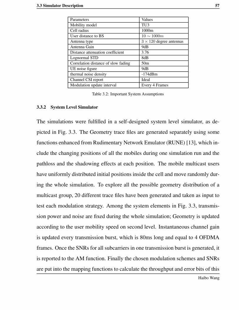
3.3 Simulator Description 57
Parameters ValuesMobility model TU3Cell radius 1000mUser distance to BS 10 ∼ 1000m
Antenna type 3 × 120 degree antennasAntenna Gain 9dBDistance attenuation coefficient 3.76Lognormal STD 8dBCorrelation distance of slow fading 50mUE noise figure 9dBthermal noise density -174dBmChannel CSI report IdealModulation update interval Every 4 Frames
Table 3.2: Important System Assumptions
3.3.2 System Level Simulator
The simulations were fulfilled in a self-designed system level simulator, as de-
picted in Fig. 3.3. The Geometry trace files are generated separately using some
functions enhanced from Rudimentary Network Emulator (RUNE) [13], which in-
clude the changing positions of all the mobiles during one simulation run and the
pathloss and the shadowing effects at each position. The mobile multicast users
have uniformly distributed initial positions inside the cell and move randomly dur-
ing the whole simulation. To explore all the possible geometry distribution of a
multicast group, 20 different trace files have been generated and taken as input to
test each modulation strategy. Among the system elements in Fig. 3.3, transmis-
sion power and noise are fixed during the whole simulation; Geometry is updated
according to the user mobility speed on second level. Instantaneous channel gain
is updated every transmission burst, which is 80ms long and equal to 4 OFDMA
frames. Once the SNRs for all subcarriers in one transmission burst is generated, it
is reported to the AM function. Finally the chosen modulation schemes and SNRs
are put into the mapping functions to calculate the throughput and error bits of thisHaibo Wang
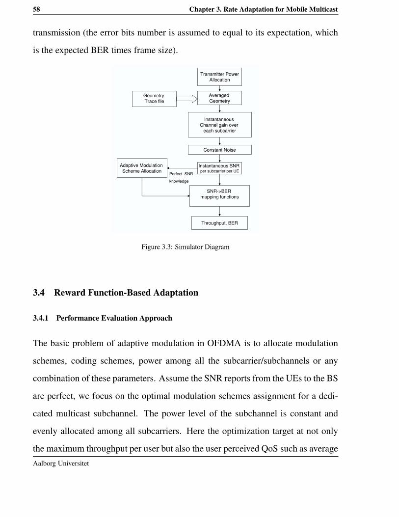
58 Chapter 3. Rate Adaptation for Mobile Multicast
transmission (the error bits number is assumed to equal to its expectation, which
is the expected BER times frame size).
Transmitter PowerAllocation
AveragedGeometry
GeometryTrace file
InstantaneousChannel gain over
each subcarrier
Constant Noise
Instantaneous SNR per subcarrier per UE
Adaptive Modulation Scheme Allocation
SNR->BERmapping functions
Throughput, BER
Perfect SNR
knowledge
Figure 3.3: Simulator Diagram
3.4 Reward Function-Based Adaptation
3.4.1 Performance Evaluation Approach
The basic problem of adaptive modulation in OFDMA is to allocate modulation
schemes, coding schemes, power among all the subcarrier/subchannels or any
combination of these parameters. Assume the SNR reports from the UEs to the BS
are perfect, we focus on the optimal modulation schemes assignment for a dedi-
cated multicast subchannel. The power level of the subchannel is constant and
evenly allocated among all subcarriers. Here the optimization target at not only
the maximum throughput per user but also the user perceived QoS such as averageAalborg Universitet

3.4 Reward Function-Based Adaptation 59
BER. The argument is that if the user perceived QoS is not at an acceptable level,
high data rate alone will not make the user satisfied. Hence we defined the Reward
function to include both:
R(T, S) = W1 × T + W2 × S (3.4)
where
S represents the user satisfaction rate defined as
S =
∑Ni=1 J(BERi ≤ θ)
N(3.5)
where J is defined as
J =
1, if condition satisfied
0, otherwise(3.6)
N is the number of mobiles in the investigated multicast group.
T represents the Normalized Average user Goodput per session, defined as:
T = (1
N
N∑
i=1
Goodputi)/Throughput256QAM
Goodputi counts only the correctly received bits by receiver i during one service
session, while
Throughput256QAM is the maximum possible throughput (always with the highest
modulation rate and error-free) for the same duration. Hence T is normalized to
be between [0, 1].
BERi refers to the average BER of receiver i during the whole multicast service
session.
θ is the average BER constraint, θ = 10−3 .
Haibo Wang

60 Chapter 3. Rate Adaptation for Mobile Multicast
W1, W2 are the relative weights of T and S in Reward function, W1 = W2 = 1,
because we consider efficiency (throughput) and QoS (BER) equally important.
Although R can reflect the joint performance of throughput and BER, it
cannot help to exclude the case that one strategy can result in a high Reward by
using extremely high modulation rate such as 256QAM and a very low satisfaction
rate where only a small portion of mobiles with high channel quality might be
satisfied, which is not the purpose of a multicast service. So we add an additional
evaluation constraint that only the strategy with S >= 50% would be considered
as a proper candidate for further performance analysis. This constraint can be
easily included in Equation. 3.4, but to better reflect the behavior of all possible
strategies we keep it separately.
3.4.2 Different Adaption Strategies
The main dilemma for a shared multicast channel is that different mobiles are ex-
periencing different SNRs but they have to listen to the same signal, which makes
it impossible to make the modulation optimal to each single mobile. The sub-
optimal modulation scheme will be to provide the highest throughput within the
BER boundary for most of the mobiles. Intuitively either the minimum, mean
or the maximum SNRs of all mobiles on each subcarrier can be chosen as the
Channel Quality Indicator to make the modulation rate selection. The drawback
is that a single SNR value cannot reflect the instantaneous SNRs distribution of
all the mobiles, hence the modulation scheme based on these strategies might not
achieve the optimal Reward. To achieve the maximal Reward value for a mul-
ticast session, we defined a Best Local Reward strategy for adaptive modulationAalborg Universitet

3.4 Reward Function-Based Adaptation 61
and compared the performance among Mean SNR based AM strategy, Best Local
Reward strategy and fixed modulation (BPSK/4QAM) strategy.
3.4.2.1 Best Local Reward Strategy
This strategy interpret the performance metric (3.4) into a Reward during each
transmission burst, and chooses the modulation mode which can maximize this
’local’ Reward, denoted as R′. To distinguish this R′ (counted per transmission)
from the performance metric, we call it Local Reward, and this AM strategy is
named Best Local Reward strategy. That is, this strategy will use instantaneous
SNR per UE per subcarrier to estimate the possible Local Reward of each mod-
ulation mode (BPSK,4/16/64/256QAM), and select the mode which maximizes
Local R′ for the current transmission burst, as illustrated in Tab.3.3:
Haibo Wang

62 Chapter 3. Rate Adaptation for Mobile Multicast
Input: SNR(i, j), i ∈ (1, ..., N).For subcarrier j = 1:32
For modulation mode M = BPSK, 4/16/64/256QAM,
S′(M, j) =1
N
N∑
i=1
J(BER(M,SNRi,j) ≤ θ);
T ′(M, j) =1
N
N∑
i=1
Kj(M)(1 − BER(M,SNRi,j))/K256QAM ;
R′(M, j) = W1 × T ′ + W2 × S′;
End;
Mopt(j) = arg maxR′(M, j);
Assign Mopt to subcarrier j;
End.BER(M,SNRi,j) : the BER of receiver i on subcarrier j, estimated from themodulation mode and SNR value.K : the number of bits per symbol of each modulation mode.S′(M, j): the local satisfaction rate of mode M on subcarrier jT ′(M, j): the local goodput of mode M on subcarrier jR′(M, j): the local Reward of mode M on subcarrier jMopt(j): the optimal modulation mode on subcarrier j
Table 3.3: The Best Local Reward Algorithm
3.4.2.2 Mean SNR Strategy
This strategy takes the average SNR among all the multicast group members over
each subcarrier, and then choose the highest modulation rate which allow the
BER(M, SNR) < θ for this subcarrier. This algorithm can be simplified as
Mode M is chosen for subcarrier j if1
N
N∑
i=1
SNRi,j ∈ [Γm, Γm+1)
where the SNR thresholds of each modulation mode, ΓM , can be derived from
Eq.3.2 and 4.12 as:
Aalborg Universitet

3.4 Reward Function-Based Adaptation 63
ΓM =
(
erfc−1(2θ))2
, K = 1 (BPSK)
− ln 5θ1.6
(
2K − 1)
, K = 2, 4, 6, 8 (4,...,256QAM)(3.7)
and the resulted SNR boundaries of each mode for θ = 10−3 are listed in Tab.
3.4.Modulation Scheme SNR Thresholds (ΓM , ΓM+1] (dB)
BPSK (−∞, 10]
4QAM (10, 17]
16QAM (17, 23]
64QAM (23, 29]
256QAM (29, + ∞)
Table 3.4: SNR Thresholds for BER < 10−3
3.4.2.3 Fixed BPSK/MQAM Strategy
As the simplest case, to always use one modulation scheme on all the subcarriers
during the whole simulation.
3.4.3 Numerical Result and Analysis
In this section we first compare the performance of different AM strategies in the
case mean(SNR) = 28dB. Then the impact of the SNR distribution on BER is
analyzed. After that, the performance from the scenario mean(SNR) = 35dB is
presented.
3.4.3.1 Performance Comparison
The following figures are the final Reward curves from different AM strategies.
While the global R in the evaluation metric keeps the same weights W1 = W2 = 1,Haibo Wang

64 Chapter 3. Rate Adaptation for Mobile Multicast
different weights combinations have been tried in R′ to reveal best weights setting
to maximize the Reward.
2 3 4 5 6 7 8 9 100.75
0.8
0.85
0.9
0.95
1
1.05
1.1
1.15Reward of BestReward,MeanSNR and BPSK,W3=W4=1
Group size in UE#
Ave
rage
Rew
ard
R, w1=w2=1R,w1=1,w2=0R,w1=0.02,w2=1Mean SNRBPSK
Figure 3.4: Reward under E(SNR) = 28dB
Surprisingly, in Fig. 3.4 it is not the R′(w′1 = w′
2 = 1) but the R′(w′1 =
1, w′2 = 0) shows the best Reward performance. The former one which keeps the
same weight setting shows a performance even worse than Mean SNR and BPSK
strategy.
To reveal the reason, the normalized throughput and satisfaction rate are also
plotted separately as in Fig. 3.5(a) and Fig. 3.5(b).
The throughput curves are as we expected: the R′(w′1 = 1, w′
2 = 0) which
only takes throughput into account achieved the highest output; the R′(w′1 = w′
2 =
1) and Mean SNR make the median ones; and the BPSK only gives the lowest out-
put. On the other hand, in Fig. 3.5(b) only the BPSK can achieve an average BER
satisfying more than half of the mobiles, according to the second requirement of
performance comparison. Other strategies all lead to the selection of a higher mod-Aalborg Universitet

3.4 Reward Function-Based Adaptation 65
2 3 4 5 6 7 8 9 100.1
0.2
0.3
0.4
0.5
0.6
0.7
0.8
0.9
1
Group size in UE#
Nor
mal
ized
Ave
rage
Thr
ough
put
Normalized Average Throughput of BestReward,MeanSNR and BPSK
R,w1=w2=1R,w1=1,w2=0R, w1=.02,w2=1Mean SNRBPSK
(a) Throughput under E(SNR) = 28dB
2 3 4 5 6 7 8 9 100
0.1
0.2
0.3
0.4
0.5
0.6
0.7
0.8
0.9
Group size in UE#
Ave
rage
Sat
isfy
rate
Average Satisfy rate of BestReward,MeanSNR and BPSK
R,w1=w2=1R,w1=1,w2=0R,w1=.02,w2=1Mean SNRBPSK
(b) Satisfaction Ratio under E(SNR) = 28dB
Figure 3.5: Throughput and satisfaction ratio (E(SNR) = 28dB)
Haibo Wang

66 Chapter 3. Rate Adaptation for Mobile Multicast
ulation rate and sacrifice the BER. In this scenario (Mean(SNR)=28dB), adaptive
strategies such as Mean-SNR based AM can achieve at most similar Reward as
BPSK. Considering the extra computational complexity and CSI feedback load
introduced by adaptive algorithms in the BS, adaptive strategies did not supply
any gain in this case.
3.4.3.2 Impact of SNR on Average BER
An average SNR of 28dB is already a very high value in the real cellular system.
To reveal why most of the strategies implemented failed to stay inside the BER
requirement under such a high mean SNR, the impact of SNR on average BER in
multicast scenario need to be analyzed. The SNR distribution of all subcarriers
from all mobiles at each transmission is depicted in Fig. 3.6. If fixed modulation
−20 0 20 40 60 800
10
20
30
40
50
60
70
80
90
100
C.D
.F.
[%]
SNR dB from all instantaneous SNR samples (dB)
SNR CDFSNR meanSNR std
Figure 3.6: Cumulative Distribution Function (CDF) of SNR, Mean=28dB,STD=11dB
schemes are used for the simulation, the average BER for each modulation from
instantaneous BERs of all SNR samples will be as shown in Tab. 3.5. This esti-
mation implies that if most of the group members are expected to have an averageAalborg Universitet
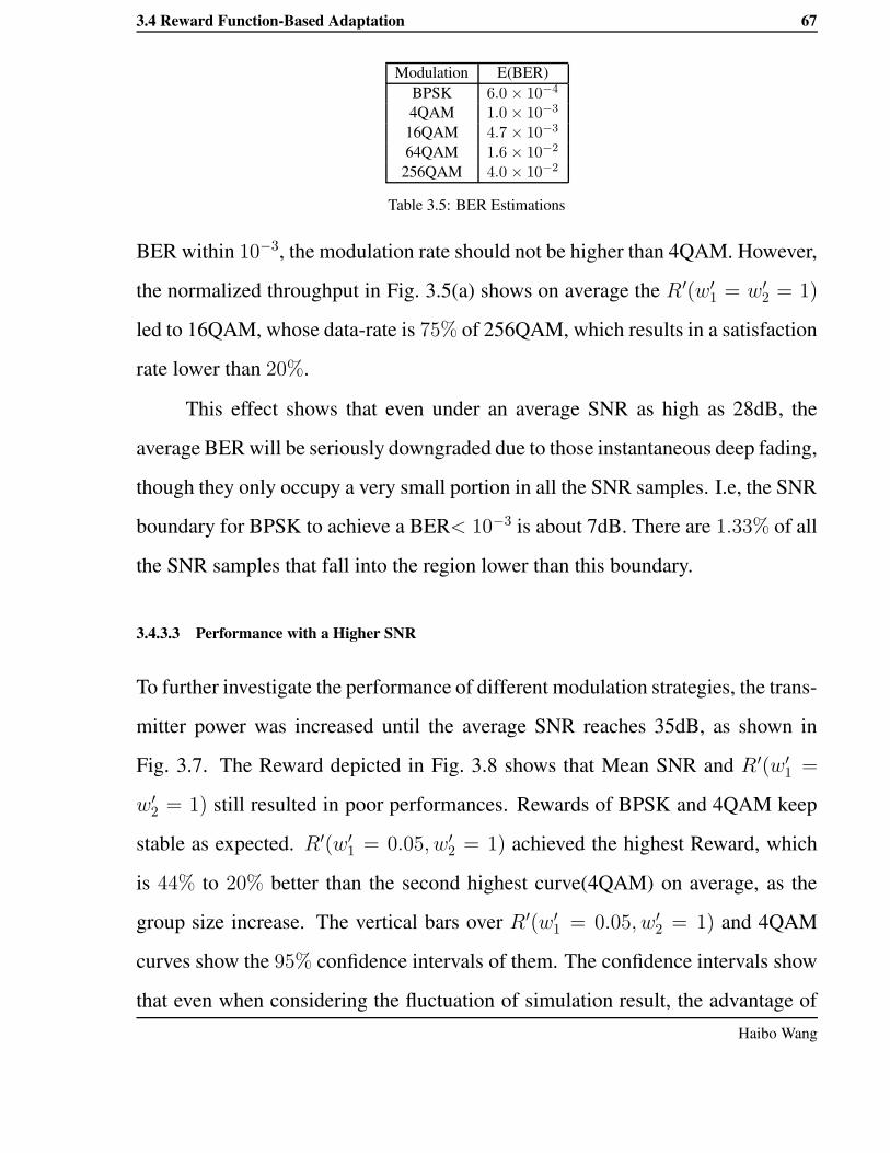
3.4 Reward Function-Based Adaptation 67
Modulation E(BER)BPSK 6.0 × 10⁻⁴
4QAM 1.0 × 10⁻³
16QAM 4.7 × 10⁻³
64QAM 1.6 × 10⁻²
256QAM 4.0 × 10⁻²
Table 3.5: BER Estimations
BER within 10−3, the modulation rate should not be higher than 4QAM. However,
the normalized throughput in Fig. 3.5(a) shows on average the R′(w′1 = w′
2 = 1)
led to 16QAM, whose data-rate is 75% of 256QAM, which results in a satisfaction
rate lower than 20%.
This effect shows that even under an average SNR as high as 28dB, the
average BER will be seriously downgraded due to those instantaneous deep fading,
though they only occupy a very small portion in all the SNR samples. I.e, the SNR
boundary for BPSK to achieve a BER< 10−3 is about 7dB. There are 1.33% of all
the SNR samples that fall into the region lower than this boundary.
3.4.3.3 Performance with a Higher SNR
To further investigate the performance of different modulation strategies, the trans-
mitter power was increased until the average SNR reaches 35dB, as shown in
Fig. 3.7. The Reward depicted in Fig. 3.8 shows that Mean SNR and R′(w′1 =
w′2 = 1) still resulted in poor performances. Rewards of BPSK and 4QAM keep
stable as expected. R′(w′1 = 0.05, w′
2 = 1) achieved the highest Reward, which
is 44% to 20% better than the second highest curve(4QAM) on average, as the
group size increase. The vertical bars over R′(w′1 = 0.05, w′
2 = 1) and 4QAM
curves show the 95% confidence intervals of them. The confidence intervals show
that even when considering the fluctuation of simulation result, the advantage ofHaibo Wang

68 Chapter 3. Rate Adaptation for Mobile Multicast
−20 0 20 40 60 800
10
20
30
40
50
60
70
80
90
100
C.D
.F.
[%]
SNR (dB)
SNR CDFSNR meanSNR STD
Figure 3.7: SNR CDF, Mean=35dB,STD=11dB
R′(w′1 = 0.05, w′
2 = 1) is still perceivable. Besides Reward, its satisfaction rate
1 2 3 4 5 6 7 8 9 10 110.8
1
1.2
1.4
1.6
1.8
2
Group size in UE#
Ave
rage
Rew
ard
Reward of BestReward,MeanSNR and Fixed strategy,W3=W4=1R, w1=w2=1R,w1=0.05,w2=1Mean SNR 256QAM64QAM4QAMBPSK
Figure 3.8: Reward under E(SNR)=35dB
also achieved over 90% as in Fig. 3.9.
Aalborg Universitet
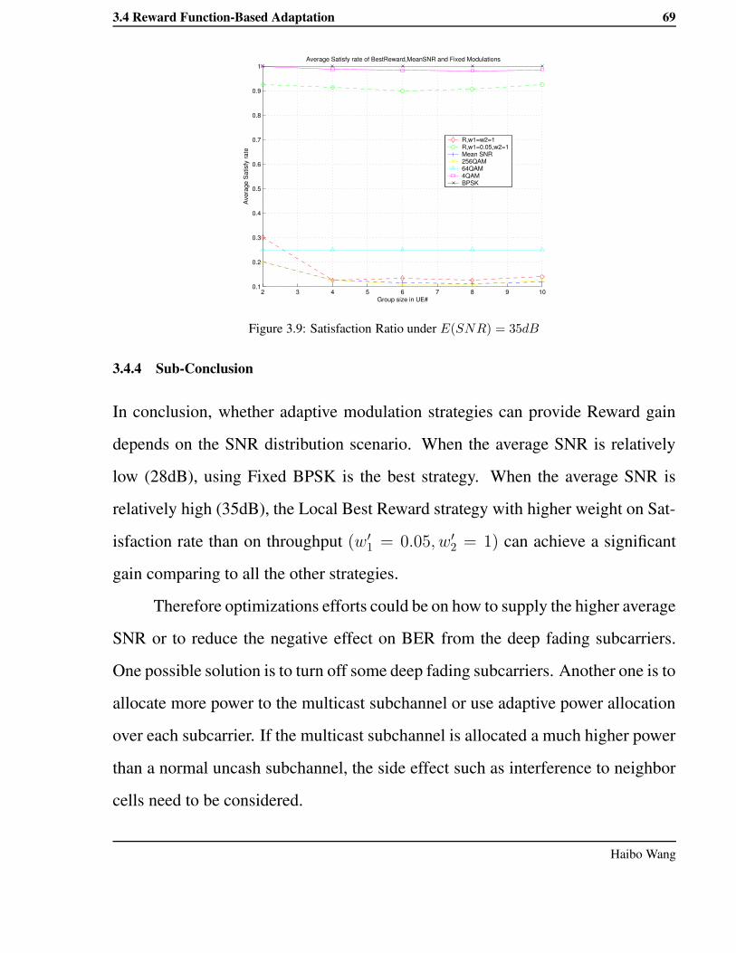
3.4 Reward Function-Based Adaptation 69
2 3 4 5 6 7 8 9 100.1
0.2
0.3
0.4
0.5
0.6
0.7
0.8
0.9
1
Group size in UE#
Ave
rage
Sat
isfy
rate
Average Satisfy rate of BestReward,MeanSNR and Fixed Modulations
R,w1=w2=1R,w1=0.05,w2=1Mean SNR256QAM64QAM4QAMBPSK
Figure 3.9: Satisfaction Ratio under E(SNR) = 35dB
3.4.4 Sub-Conclusion
In conclusion, whether adaptive modulation strategies can provide Reward gain
depends on the SNR distribution scenario. When the average SNR is relatively
low (28dB), using Fixed BPSK is the best strategy. When the average SNR is
relatively high (35dB), the Local Best Reward strategy with higher weight on Sat-
isfaction rate than on throughput (w′1 = 0.05, w′
2 = 1) can achieve a significant
gain comparing to all the other strategies.
Therefore optimizations efforts could be on how to supply the higher average
SNR or to reduce the negative effect on BER from the deep fading subcarriers.
One possible solution is to turn off some deep fading subcarriers. Another one is to
allocate more power to the multicast subchannel or use adaptive power allocation
over each subcarrier. If the multicast subchannel is allocated a much higher power
than a normal uncash subchannel, the side effect such as interference to neighbor
cells need to be considered.
Haibo Wang

70 Chapter 3. Rate Adaptation for Mobile Multicast
3.5 History-Based BER Threshold Adaptation
The previous section reveals that the system performance is limited by the worst
SNRs. If the adaptation strategy allows some instantaneous errors for the mul-
ticast receivers in a temporary deep fading, higher data rate can be allocated to
the group and higher goodput may be achieved eventually. Since the deep fading
stage of a receiver is only temporary, the average BER can still be controlled at
an acceptable level in long term. That is, we propose an approach to keep track
of cumulative errors of each receiver and optimistically adapt modulation for the
multicast transmission, which we called a history-based adaptive modulation.
3.5.1 Performance Evaluation Metric
In the previous section, a Reward function is defined to include both throughput
and BER, and the simulation results reflect the tradeoff between them. That is,
throughput and BER cannot be maximized together, and the improvement of one
always compromise the other. Hence we redefine the optimization target to maxi-
mizing the throughput while keeping the average BER constraint for the multicast
group, and adopt a modified Reward function (R) as:
For a multicast service session,
R = T · S (3.8)
and
S = J
(
∑N
i=1J(BERi ≤ θ)
N≥ µ
)
(3.9)
Aalborg Universitet

3.5 History-Based BER Threshold Adaptation 71
where J has been defined in Eq. 3.6, T has been defined in Eq. 3.4.1.
µ stands for the required percentage of multicast group members within BER con-
straint. In this section, the target percentage is µ = 1, then
R =
T, if, for all i, BERi ≤ θ
0, otherwise(3.10)
3.5.2 Different Adaptation Strategies
Three AM strategies are compared in this section. Based on the sub-conclusion of
Sec. 3.5, sub-carrier turnoff is adopted in each strategy.
(1) Best Local Reward Strategy with Fixed BER Threshold
Similar to the Local Reward strategy in the previous section, this strategy select
the modulation mode which maximize the Local Reward R′.
This Best Reward function simply uses a fixed instantaneous BER constraint,
θ. Assume receiver i had the lowest SNR on subcarrier j, and M is the highest
modulation mode satisfying BER(M, SNRi,j) ≤ θ (which means BER(M +
1, SNRi,j) > θ). Then according to the definition of R’, R′(M) > 0 and R′(M +
1) = 0, the Best Reward algorithm will choose M. Therefore, on each subcarrier
the lowest SNR among all receivers will limit the choice of modulation mode,
which is a kind of adapt-to-worst strategy.
Comparing to the definition of R in the previous section, S has much stronger
influence in the current R function. In the previous R, lower S may be compen-
sated by higher T ; whereas the current R will switch between T and 0 depending
on S. Therefore the new Best Local Reward strategy is even more conservativeHaibo Wang

72 Chapter 3. Rate Adaptation for Mobile Multicast
Input: SNR(i, j), i ∈ (1, ..., N).For subcarrier j = 1:32
If ∃ SNRi,j < ΓBPSK(θ)
Turn off subcarrier j,Else
For modulation mode M = BPSK, 4/16/64/256QAM,
T ′(M, j) =Kj(M)
K256QAM× 1
N
∑
i
[1 − BER(M,SNRi,j)]
R′(M, j) =
T ′(M, j), if, for all i, BERi,j ≤ θ0, otherwise
End;
Mopt(j) = arg max R′(M, j);
Assign Mopt to subcarrier j;
End;End.
Table 3.6: The Best Local Reward Algorithm with Fixed BER Threshold
than the one in previous section, and more optimistic adaptation strategy should
be proposed.
(2) Reward strategy with Adaptive BER Threshold
The further proposal is to allow the instantaneous BER boundary to be varied to
achieve higher throughput, and still keep the average BER within θ. Therefore,
it is necessary to keep track of the cumulated BER, BERc(i), for each mobile
individually, and adapt the θt(i) (instantaneous BER constraint for mobile i at
transmission t) according to BERc. That is, the calculation of the local Reward
of each possible modulation becomes
R′(M) =
T, if, for all i, BERi ≤ θt(i)
0, otherwise
Aalborg Universitet

3.5 History-Based BER Threshold Adaptation 73
This idea is implemented in an Adaptive BER Threshold Algorithm, inspired by
[14].1 The coordination procedure between the Best Reward algorithm and the
Adaptive BER Threshold Algorithm is illustrated in Fig. 3.10. The Best Local
Reward function is mostly the same as in Tab.3.6, except each θ in the former is
replaced by θt(i). The Best Reward function will start with the same θt(i) = θ, and
the transmission result will be reported to the Adaptive BER Threshold Algorithm
to decide θt+1(i) to be used by the Best Reward for the next transmission. In this
way the BER history knowledge of each user is utilized: when a receiver has the
worst SNR on subcarrier j at transmission time t, but it has a good average BER
so far, it can have a higher BER limit than θ and the modulation mode allocated
for the whole group can be higher.
Instantaneous SNR
information
Best Reward
Modulation Allocation
Transmission
Throughput, BER
Heuristic t(i)Adaption :
Update BERc,
Modify t(i) accordingly
t(i)
Figure 3.10: Best Reward AM with Heuristic BER Constraint
1The work in Chapter 3 was inspired by the work in [14] in terms of varying a certain criteria in time domain. But the workin [14] is about access control according to the instantaneous cell load (session arrival, leaving, handover), with Markov chainanalysis. The optimization scenario (session level V.S. transmission burst level), target metric, RRM approach (access control V.S.link adaptation) and corresponding parameters are totally different. This history-based BER threshold scheme is novel in the fieldof link adaptation.
Haibo Wang

74 Chapter 3. Rate Adaptation for Mobile Multicast
Adaptive BER Threshold Algorithm
The important variables and parameters in this algorithm are:
BERc(i) :Number of error bits received
Number of bits receivedby UEi from the transmission starts to current time;
θ1: The arbitrary lower boundary of the optimal BER interval;
θt(i): Instantaneous BER Threshold for the next transmission for UEi, initially
θt(i) = θ;
θmax: Maximum allowed value of θt(i);
δ: The multiplicative factor to increase θt(i).
For i = 1 : N % for each multicast group memberupdate BERc(i) based on the previous transmission output;IF 0 < BERc(i) < θ1 THEN
% BER too good, loose thresholdθt(i) = min(θt(i) × δ, θmax)
ELSE IF BERc(i) > θ THEN% BER break boundary, tight thresholdIF θt(i) > θ , THEN
θt(i) = θ;End
ELSE IF θ1 ≤ BERc(i) ≤ θ,This is the optimum case, keep θt(i) unchanged.
EndEnd.
Table 3.7: Adaptive BER Threshold Algorithm
There are two states in this instantaneous BER threshold varying process:
the maximizing utilization state and the compensation state. In the maximizing
utilization state, θt(i) will be temporarily increased to gain higher data rate. If
BERc(i) becomes greater than θ afterward, the algorithm will switch to compen-
sation state. In the compensation state the where θt(i) will be decreased, which
should result in less instantaneous errors in subsequent bursts until the BERc fallAalborg Universitet
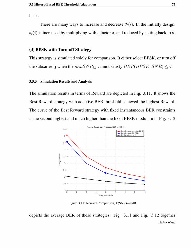
3.5 History-Based BER Threshold Adaptation 75
back.
There are many ways to increase and decrease θt(i). In the initially design,
θt(i) is increased by multiplying with a factor δ, and reduced by setting back to θ.
(3) BPSK with Turn-off Strategy
This strategy is simulated solely for comparison. It either select BPSK, or turn off
the subcarrier j when the minSNRi,j cannot satisfy BER(BPSK, SNR) ≤ θ.
3.5.3 Simulation Results and Analysis
The simulation results in terms of Reward are depicted in Fig. 3.11. It shows the
Best Reward strategy with adaptive BER threshold achieved the highest Reward.
The curve of the Best Reward strategy with fixed instantaneous BER constraints
is the second highest and much higher than the fixed BPSK modulation. Fig. 3.12
2 3 4 5 6 7 8 9 100
0.05
0.1
0.15
0.2
0.25
0.3
0.35
0.4
0.45
Group size in UE#
Ave
rage
Rew
ard
Reward Comparison, R=goodput|BER <= 10E−3
Best Reward, adaptive BERBest Reward, Fix BERBPSK with turn−off
Figure 3.11: Reward Comparison, E(SNR)=20dB
depicts the average BER of these strategies. Fig. 3.11 and Fig. 3.12 togetherHaibo Wang

76 Chapter 3. Rate Adaptation for Mobile Multicast
reflect the trade-off between average BER and Reward. Best Reward with adap-
tive BER strategy achieved the highest Reward by pushing the average BER level
closer to 10−3, while Best Reward with fixed instantaneous BER result in the BER
level nearly 10−4 and lower Reward. The BPSK scheme, provided the best reli-
ability and the worst Reward as expected. Theoretically it should be possible to
push this BER curve even closer to 10−3 by algorithm optimization or parameter
optimization, to achieve the highest Reward.
2 3 4 5 6 7 8 9 1010−6
10−5
10−4
10−3
Group size in UE#
Ave
rage
BE
R
BR adaptive BERBR fixed BERBPSK with turn−off
Figure 3.12: Average BER Comparison, E(SNR)=20dB
3.5.3.1 Impact of Group Size
In Fig. 3.11 all the Reward curves go down as the group size increase. Because the
more users in a group, the higher probability that one of them subjects to deep fad-
ing which results in SNRs even lower than the threshold of BPSK. Though there
is also higher probability that some members get higher SNR at the same time,
they cannot impact on the modulation selection as the lowest SNR can do. TheAalborg Universitet

3.5 History-Based BER Threshold Adaptation 77
2 3 4 5 6 7 8 9 100.05
0.1
0.15
0.2
0.25
0.3
0.35
0.4
0.45
Group size in UE#
Ave
rage
Rew
ard
Delta=2, theta1=.99E−3Delta=4, theta1=.99E−3Delta=10, theta1=.99E−3
Figure 3.13: Impacts of δ Settings on Adaptive BER Algorithm, E(SNR)=20dB
proposed Best Reward with BER adaption algorithm achieved higher gain as the
group size increases, i.e, its Reward values are 13.5%, 25.6%, 30.3%, 32.5%, 34.4%
higher than those of Best Reward with Fixed BER Threshold strategy at the group
sizes (2, 4, 6, 8, 10), respectively.
3.5.3.2 Impact of Parameters Setting
The parameter δ decides the speed to loosen θt(i). We start with the simplest
case that δ = 10, which means θt(i) only needs to switch between θ and θmax.
Other initial settings of this algorithm are: θ1 = 0.99 × 10⁻³ and θmax = 10−2.
The results in Fig. 3.11 and Fig. 3.12 came from these initial settings. Later
some selective input parameter sets are also tested to reveal their impact on the
performance of Best Reward with Adaptive BER algorithm, as shown in Fig. 3.13
and 3.14. Fig. 3.13 shows that stepwise adaptation of θt(i) (e.g.,δ = 2, 4) did not
further improve Reward gain comparing to the simplest case δ = 10. On the otherHaibo Wang

78 Chapter 3. Rate Adaptation for Mobile Multicast
2 3 4 5 6 7 8 9 100.15
0.2
0.25
0.3
0.35
0.4
0.45
0.5
Group size in UE#
Ave
rage
Rew
ard
Delta=10, Theta1=0.99E−3Delta=10, Theta1=0.9E−3Delta=10, Theta1=0.6E−3
Figure 3.14: Impacts of θ1 Settings on Adaptive BER Algorithm, E(SNR)=20dB
hand, different θ1 settings only have minor impact on R as presented in Fig. 3.14,
mainly on the small group size case (2 users only). Therefore it is better to simply
switch θt(i) between θ and θmax.
3.5.3.3 Spectrum Efficiency Gain
When we interpret the result back to spectral efficiency, it is counted from a cell
perspective how much information has been effectively served to multicast users
per unit bandwidth, calculated as
∑Ni=1 Successfully received bits/sec of UEi
Bandwidth of the multicast channel
The result in Fig. 3.15 verified that the spectral efficiency of the proposed AM
algorithm outperforms the others, and it can gain as high as 6.58 bps/Hz compar-
ing to the Best Reward with Fixed Threshold algorithm at large group size. In
this figure the curve of the Best Reward with Fixed Threshold strategy is not in-Aalborg Universitet

3.6 Conclusion 79
1 2 3 4 5 6 7 8 9 10 110
2
4
6
8
10
12
Group size in UE#
Spe
ctru
m E
ffici
ency
(bps
/Hz)
Best Reward, adaptive BER,Delta=10, theta1=.99E−3 Fix ThresholdBPSK with turn−off
1.14 bps/Hz
6.58bps/Hz
3.64bps/Hz
1.88bps/Hz
Figure 3.15: Spectrum Efficiency of AM Strategies, E(SNR)=20dB
creasing monotonically, meaning the loss in average throughput may not always
be compensated by the increment of group members.
3.5.4 Sub-Conclusion
In this section, the Best Reward with Adaptive BER threshold algorithm opti-
mistically relaxes the instantaneous BER constraints based on the BER history of
each multicast user, and achieves large performance gain. The proposed algorithm
shows even bigger advantage comparing to other strategies when the group size is
large.
3.6 Conclusion
In this chapter the OFDM-based AM approaches are studied with Reward func-
tions as performance metrics. The Reward functions are designed in order to in-
clude both the throughput and the average BER per multicast receiver (in termsHaibo Wang

80 Chapter 3. Rate Adaptation for Mobile Multicast
of satisfaction rate S). It is more convenient to include BER in the Reward func-
tion of Sec. 3.5 than in the Reward of Sec. 3.4, since it is not easy to decide what
weight settings for throughput and satisfaction rate would be the best.
A few AM schemes are proposed and their performances are compared via
simulations. For the first Reward function, the simulation results show that it is
necessary to turn off the subcarriers where some receivers are in deep fading, since
these cases degrade the satisfaction rate seriously. Without subcarrier turnoff, the
Best Local Reward strategy only outperform other AM schemes when the average
SNR is very high. For the second Reward function, all the AM schemes adopt sub-
carrier turnoff option, and a history-based BER threshold adaptation is proposed
to cooperate with the Best Local Reward strategy. Simulation results prove that
this new proposal gain extra performance in both Reward and spectral efficiency
by comprising the average BER, but still keep the BER constraint inviolated.
Based on the work of this chapter, further optimization efforts can be made
in the following directions:
Defining more objective performance metric The design of a precise Reward
function for mobile multicast services should better be supported the data
from mobile network operators or service providers. As it is difficult to get
such data, researchers often propose different Reward functions for the same
problem and the outputs are difficult to compare. So it is better to use more
objective performance metrics, which also reflect both throughput and BER,
for further optimization.
Investigation method The investigation in this chapter is based on simulations,
which include many detailed parameter settings, and the results and conclu-Aalborg Universitet

3.6 Conclusion 81
sions are rather specific to such a simulation scenario. Even though the sim-
ulation can be repeated for different parameters settings, when the number of
parameters is large or when the simulation is time-consuming , it is impossi-
ble to tryout many different parameters combinations. In this case, it is hard
to predict the possible behaviors of the investigated algorithms in different
scenarios, or to explain why some behaviors happen. Hence further work can
be done to build analytical models.
More degrees of freedom Beside rate adaptation, power adaptation should also
be investigated together for multicast link adaptations.
Note: The works presented in this chapter have been published in [15] and [16].
Haibo Wang

Bibliography
[1] M. Hauge and Ø. Kure, “Multicast in 3G Networks: Employment of Exist-
ing IP Multicast Protocols in UMTS,” in The Fifth International Workshop on
Wireless Mobile Multimedia (WoWMoM 2002), Atlanta, USA, Sept. 2002,.
[2] Y. Silva and A. Klein, “Adaptive Beam-forming and Spatial Multiplexing
of Unicast and Multicast Services,” in The 17th Annual IEEE International
Symposium on Personal, Indoor and Mobile Raido Communications (PIMRC
2006), Helsinki, Finland, Sept. 2006.
[3] J. L. Brito, A. Correia and A. Adetti, “Wireless techniques for capacity en-
hancement of broadcast and multicast for UMTS networks,” in IEEE Vehicular
Technology Conference 2004 (VTC’04-Fall), Los Angeles, USA, Sept. 2004.
[4] Y. Sun and K. J. R. Liu, “Transmit diversity techniques for multicasting over
wireless networks,” in Wireless Communications and Networking Conference
2004 (WCNC’04), Atlanta, USA, March 2004.
[5] K. Mori, K. Naito, H. Kobayashi and H. Aghvami, “Dynamic Subband and
Code Channel Assignment for Multicast Band Division MC-CDMA Systems,”82

BIBLIOGRAPHY 83
in The 17th Annual IEEE International Symposium on Personal, Indoor and
Mobile Raido Communications (PIMRC 2006), Helsinki, Finland, Sept. 2006.
[6] C. Y. Wong, R. S. Cheng, K. B. Letaief and R. D. Murch, “Multiuser OFDM
with Adaptive Subcarrier, Bit, and Power Allocation,” in IEEE Journal on
Selected Areas in Communications, vol. 17, no. 10, pp. 1747-1758, Oct. 1999.
[7] S. Pietrzyk, G. J. M. Janssen, “Multiuser Subcarrier Allocation for QoS Pro-
vision in the OFDMA Systems,” in IEEE Vehicular Technology Conference
2002 (VTC’02-Fall), Vancouver, Canada, Sept. 2002.
[8] E. Lawrey, “MULTIUSER OFDM,” in International Symposium on Signal
Processing and its Applications 1999 (ISSPA’99), Brisbane, Australia, Aug.
1999.
[9] N. Jindal, Z.Q.Luo, “Capacity Limits of Multiple Antenna Multicast,” in
IEEE International Symposium on Information Theory 2006 (ISIT’06), Seat-
tle, USA, July 2006.
[10] J. Nonenmacher, E. Biersack, and D. Towsley, “Parity-based Loss Recovery
for Reliable Multicast Transmission,” in ACM Trans. Networking, vol. 6, no.
4, pp. 349-361, Aug. 1998.
[11] S. T. Chung, A. J. Goldsmith, “Degrees of Freedom in Adaptive Modulation:
A Unified View,” in IEEE Trans. Commun., vol. 49, no. 9, pp. 1561-1571,
Sept. 2001.
[12] S. Yoon, C. Suh, Y. Cho and D. S. Park, “Orthogonal Frequency Division
Multiple Access with an Aggregated Sub-channel Structure and StatisticalHaibo Wang

84 BIBLIOGRAPHY
Channel Quality Measurement,” in IEEE Vehicular Technology Conference
2004 (VTC’04-Fall), Los Angeles, USA, Sept. 2004.
[13] Zander.J and S.L.Kim, Radio Resource Management for Wireess Networks,
Artech House, 2001, ISBN 1-58053-146-6
[14] J. Y. Lee, J. Choi, K. Park, and S. Bahk, “Realistic Cell-oriented Adaptive
Admission Control for QoS Support in Wireless Multimedia Networks,” in
IEEE Trans. on Vehicular Tech., 52(3), May 2003.
[15] H. Wang, H. P. Schwefel and T. T. Nielsen, “Adaptive Modulation for a
Downlink Multicast Channel in OFDMA systems,” in Proc. IEEE Wireless
and Networking Conference (WCNC’07), HongKong, China, Mar. 2007.
[16] H. Wang, H. P. Schwefel and T. S. Toftegaard, “History-based Adaptive
Modulation for a Downlink Multicast Channel in OFDMA systems,” in Proc.
IEEE Wireless and Networking Conference (WCNC’08), Las Vegas, USA,
Mar. 2008.
Aalborg Universitet

Chapter 4
Multi-Dimensional Optimization with
Analytical Model
The optimization approaches in the previous chapter are analyzed with simula-
tions tools. When comparing different multicast link adaptation schemes, it is
interesting to know the optimum performance limits of them, and to analytically
reveal why some adaptation approaches are better than others. In this chapter,
we assume a single carrier system and build an analytical framework to find out
the achievable spectrum efficiency upper boundary of such a scenario. The op-
timal and sub-optimal adaptation schemes are derived under this framework and
detailed parameter analysis are fulfilled. The problem of switching-threshold be-
tween unicast and multicast is also investigated in this chapter.
4.1 Motivation
The basic constraint in physical layer multicast adaptation is that, given a cer-
tain Bit-Error-Ratio (BER) constraint, the instantaneous transmission mode has
to adapt to the worst instantaneous channel state among all the receivers, namely85
86 Chapter 4. Multi-Dimensional Optimization with Analytical Model
worst-channel-limit. The investigations in [2], [4] and [3] propose approaches with
MIMO and Beam-forming techniques to improve the worst channel condition of
a multicast group, whereas the work in [3] develops rate adaptation schemes for
multicast in OFDM systems. These approaches can certainly improve the multi-
cast performance, but do not reveal what is the best possible adaptation scheme in
their scenarios. Some other works propose theoretical approaches for optimal rate
and/or power adaptation based on the Shannon capacity ([9], [1], [2]). However,
the Shannon capacity requires some ideal assumptions which could be far from
the constraints in reality[4]. For example, according to Shannon capacity
CB = log2(1 + SNR) (4.1)
where C is the ideal channel capacity in bit/s and B is the transmission bandwidth
in Hz, and C/B is the ideal spectral efficiency in bit/s/Hz. The achievable spectral
efficiency of practical modulation schemes can be estimated as
RB = log2(1 +
SNR
Υ). (4.2)
where R is the data rate of practical modulations (e.g., QAM), Υ represent a ’gap’
between Shannon capacity and the achievable capacity of real modulations and it
is not constant. Hence the optimal multicast performance and the corresponding
adaptation strategy from information theory perspective may not be achievable.
Another issue related to the worst-channel-limit is, since multicast adapta-
tion cannot be as efficient as unicast adaptation for each receiver itself, whether it
is always worth switching from multiple unicast to multicast mode even when the
group size is small (e.g., only two-receivers-group).Aalborg Universitet

4.2 Single-Carrier System Model 87
To address these efficient multicast issues, we investigate the average mul-
ticast spectral efficiency per receiver with different combinations of the transmit
power and rate adaptations. We assumed the investigated adaptation strategies are
subject to an average power and instantaneous BER constraints. The data rate is
adaptable due to varied modulation constellations, but the effect of adaptive chan-
nel coding is not considered. We first investigate the power and rate adaptation
given the modulation constellations can be varied continuously, and then analyze
the more realistic scenario where only a discrete set of constellations as well as
data rate are available.
4.2 Single-Carrier System Model
Based on the general assumptions described in Chapter 1, the transceiver system
is now assumed as a single carrier system. The channel models of N multicast
receivers are assumed as discrete-time flat-fading channels, with stationary and
ergodic time-varying gain and Additive White Gaussian Noise (AWGN). Since
the channel gains are stationary, the distributions of them are independent of time
and the time reference is omitted in our expressions. The received symbols at the
i-th multicast receiver, denoted as yi, can be characterized as
yi = gix + ni, i = 1, ..., N (4.3)
where x is the transmitted Multicast symbols, gi is the channel gain of receiver i
and ni is the additive white Gaussian noise with variance σi2. Hence the SNR of
each receiver at each time-slot can be written asHaibo Wang
88 Chapter 4. Multi-Dimensional Optimization with Analytical Model
SNRi =S|gi|2σi
2(4.4)
in which S is the transmission power. Assume the average transmission power is
S, and the received instantaneous SNRs under this power level are
γi =S · |gi|2
σi2
, (4.5)
which can be measured by the receivers (i.e, with the help of the pilot channel).
In this work, γi is called Normalized SNR and taken as the main channel quality
indicator. We further assume that the receivers can detect their γi under this con-
stant power level, i.e, by measuring the signal in the downlink pilot signal, and
report them in a non-delay and error-free feedback channel. The base station ful-
fills downlink power control according to γi(i = 1..N) and transmits the Multicast
content with instantaneous power S. Therefore the actually received SNRs of each
time-slot can be rewritten as
SNRi =S
S· S · |gi|2
σi2
=S
S· γi (4.6)
The Probability Density Functions (PDFs) of γi follow Independent Identical Dis-
tributions (i.i.d), noted as p(γi). The random vector ~γ := (γ1, γ2, ..., γN) rep-
resents a fading state of the Multicast group, with probability density function
p∗(~γ) =∏N
i=1 p(γi).
As introduced in the first section, we are looking for the optimal power S
(watt) and rate k (bits/ symbol) adaptation schemes to maximize the spectral effi-
ciency. S is assumed to be continuous non-negative function of the instantaneousAalborg Universitet

4.3 Problem Formulation 89
channel fading state ~γ, noted as S(~γ). The average level of S is limited to be no
more than S to control the interference of the multicast channel toward other cells.
k is a non-negative function of ~γ, noted as k(~γ), which can be either continuous or
discrete. Besides, the multicast channel can also be turn-off in some fading states,
where S = 0 and k = 0.
The BER constraint could be either average or instantaneous, depend on
the characters of the service investigated. Given the instantaneous BER limit,
the transceiver system has to guarantee that the probability of bit error in each
channel state is no more than a constant value; whereas under the average BER
constraint, only the BER level averaged along time or channel fading states need
to be maintained, and the BER limit for different channel states could be differ-
ent. In providing real-time multimedia services via multicast, it is crucial to keep
a low instantaneous frame error ratio (FER) for good user-perceived quality of
services. Instantaneous FER can be derived from instantaneous BER, therefore a
instantaneous BER constraint is chosen in our investigation.
4.3 Problem Formulation
The optimization target is the average spectral efficiency per multicast receiver,
which equals the average data rate per unit bandwidth. When the signal is sent at
modulation mode M with k bits/symbol, the instantaneous data rate R = k/Ts
bps, where Ts is the symbol time. Under Nyquist sample rate B = 1/Ts , hence
R = k · B, and the instantaneous spectral efficiency becomes
RB = k.
Haibo Wang

90 Chapter 4. Multi-Dimensional Optimization with Analytical Model
The mathematical expectation of the spectral efficiency on the transmitter side is
the instantaneous spectral efficiency averaged over all possible fading states, noted
as (R/B)T ,
(RB )T =
∫
(R+
0 )N
k(~γ)p∗(~γ)d~γ (4.7)
(~γ) in Eq.4.7 and all the following integrations is in linear unit, hence it is always
integrated in (R+0 )N , a N-dimensional space of positive real numbers. Considering
the errors introduced by the wireless channel, the spectrum efficiency at receiver i
is
(RB )i =
∫
(R+
0 )N
k(~γ)p∗(~γ) [1 − BERi(k(~γ), S(~γ), ~γ)]d~γ (4.8)
and the average spectral efficiency of the multicast receivers should be
(RB ) =
1
N
N∑
i=1
∫
(R+0 )N
k(~γ)p∗(~γ) [1 − BERi(k(~γ), S(~γ), ~γ)] d~γ (4.9)
Likewise the average power constraint over all fading states is
ES(~γ) :=
∫
(R+0 )N
S(~γ)p∗(~γ)d~γ ≤ S. (4.10)
For a multicast group, there exist N instantaneous BER constraints:
BERi(k(~γ), S(~γ), ~γ) ≤ θ, (4.11)
where θ represent the required BER constraint value (e.g., 10−3 or 10−6).
Aalborg Universitet

4.3 Problem Formulation 91
An instantaneous BER estimation for un-coded MQAM [4] is employed for
the continuous k:
BERi ≈ 0.2 exp(−1.6γi
S(~γ)
S
2k(~γ) − 1) (4.12)
It needs to be mentioned that this estimation is tight only when γi · S(~γ)
S≥ 1.
The instantaneous BER constraint is a rather strong limitation, since the er-
ror probability scale exponentially to SSγi as shown in Eq. (4.12). It would be wise
to turn off the transmission rather than assign huge power and very low rate to meet
θ when the fading state is too bad. That is, we can assume a region Ω ⊂ (R+0 )N
such that k and S are positive functions if and only if ~γ ∈ Ω, and zero otherwise.
More detailed discussion on this region will be presented in the following sections.
Problem Simplification
To reduce the complexity of maximizing Eq.(4.9), some simplifications are made.
Typically θ is a very small value, and if this constraint holds during the transmis-
sion, the difference between the spectrum efficiency at transmitter side and re-
ceiver side is negligible. Therefore, the maximization target can be approximated
as
(RB ) ≈
∫
(R+0 )N
k(~γ)p∗(~γ)d~γ. (4.13)
We take Eq.4.13 as the estimation of the average spectrum efficiency of the multi-
cast group to be maximized, for simplicity (RB ) is just written as RB in the following
sections.
To ensure instantaneous BERi ≤ θ, it must be guaranteed that
maxBERi(k(~γ), S(~γ), ~γ) = θ,
Haibo Wang

92 Chapter 4. Multi-Dimensional Optimization with Analytical Model
which equals to BER(min~γ) = θ. This is exactly the adapt-to-worst case. With
this simplification we can derive from Eq.(4.12):
k(~γ) = log2
[
1 −1.6 min~γ S(~γ)
S
ln(5θ)
]
, S > 0. (4.14)
4.4 Solutions with Continuous Rate Adaptation
In this section we apply Lagrange method to derive the optimal spectral efficiency
and corresponding rate and power solutions, given the transmission data rate k can
be continuously adapted to the channel conditions. A sub-optimal solution with
constant power and other alternative solution are also developed and analyzed for
comparison.
4.4.1 Adaptation Schemes
4.4.1.1 Optimal Power and Continuous Rate Adaptation (CRSopt)
Using the expansion of k(~γ) in Eq.(4.14), the N instantaneous BER constraints
can be dropped and it remains to look for S such that the integral in Eq.(4.7) is
maximized under the power constraint Eq.(4.10). Eq.(4.7) can be re-written in the
form
∫
(R+
0 )N
k(~γ)p∗(~γ)d~γ
=
∫
(R+
0 )N
log2
[
1 −1.6 min~γ S(~γ)
S
ln(5θ)
]
p∗(~γ)d~γ
=:
∫
(R+
0 )N
g(S(~γ), ~γ)d~γ (4.15)
Aalborg Universitet

4.4 Solutions with Continuous Rate Adaptation 93
We construct the Lagrange function of this problem as
J (S(~γ), ~γ) :=
∫
(R+
0 )N
g(S(~γ), ~γ)d~γ
+ λ0
[∫
(R+
0 )N
S(~γ)p∗(~γ)d~γ − S
]
(4.16)
The problem reduces to find the optimal function S(~γ) with the average power S
limit.
Define
I(ε) := J (S + εσ)
where σ is an arbitrary function and ε is a small enough number. Given the optimal
S(~γ) exists, there should be
∀ ε, I(ε) ≤ I(0) =⇒ dIdε
(0) = 0.
Eq.(4.15),(4.16),(4.4.1.1) and condition dIdε (0) = 0 lead to
1.6
ln 2· min~γ1.6 · min~γS − S ln(5θ)
+ λ0 = 0,
∀ σ, and for all ~γ such that p∗(~γ) 6= 0.
Hence the theoretical optimal power scheme, noted as Sopt(~γ), is
Sopt(~γ) =c S
min~γ − 1
λ0 ln 2(4.17)
where c = ln 5θ/1.6.
For an practical instantaneous BER limit (usually 10−3 ∼ 10−6), there must
be θ < 0.2 → c < 0, hence Sopt is a monotonically increasing function ofHaibo Wang

94 Chapter 4. Multi-Dimensional Optimization with Analytical Model
min~γ, ~γ. Since γi are i.i.d. we can assume Ω has the form [γ0, +∞)N , where
γ0 is the threshold for transmission turn-on/turn-off.
Then it should be possible to find the region Ω in (R+0 )
N , in which min~γ ≥γ0, and substitute S(~γ) in Eq.(4.10) with Eq.(4.17) and take the upper-limit of the
power, we get∫
Ω
[c S
min~γ − 1
λ0 ln 2]p∗(~γ)d~γ = S (4.18)
Let
∆ :=
∫
Ω
p∗(~γ)
min~γd~γ (4.19)
α :=
∫
Ω
p∗(~γ)d~γ (4.20)
→ λ0 =α
S ln 2 · [c∆ − 1]
which leads to
S
S=
cmin~γ + 1−c∆
α, min~γ ≥ γ0
0, otherwise.(4.21)
And use (4.21) in (4.14)
k =
log2
(
c∆−1αc min~γ
)
, min~γ ≥ γ0
0, otherwise.(4.22)
The optimal spectrum efficiency can be computed by
R
B=
∫
Ω
log2
(
c∆ − 1
αcmin~γ
)
p∗(~γ)d~γ (4.23)
So far we derived the general form of the optimal S and k allocation schemes, and
the problem remains how to find the value of α and ∆, which depend on the region
Ω. As we have assumed Ω has the form [γ0, +∞)N , searching for the proper Ω
Aalborg Universitet
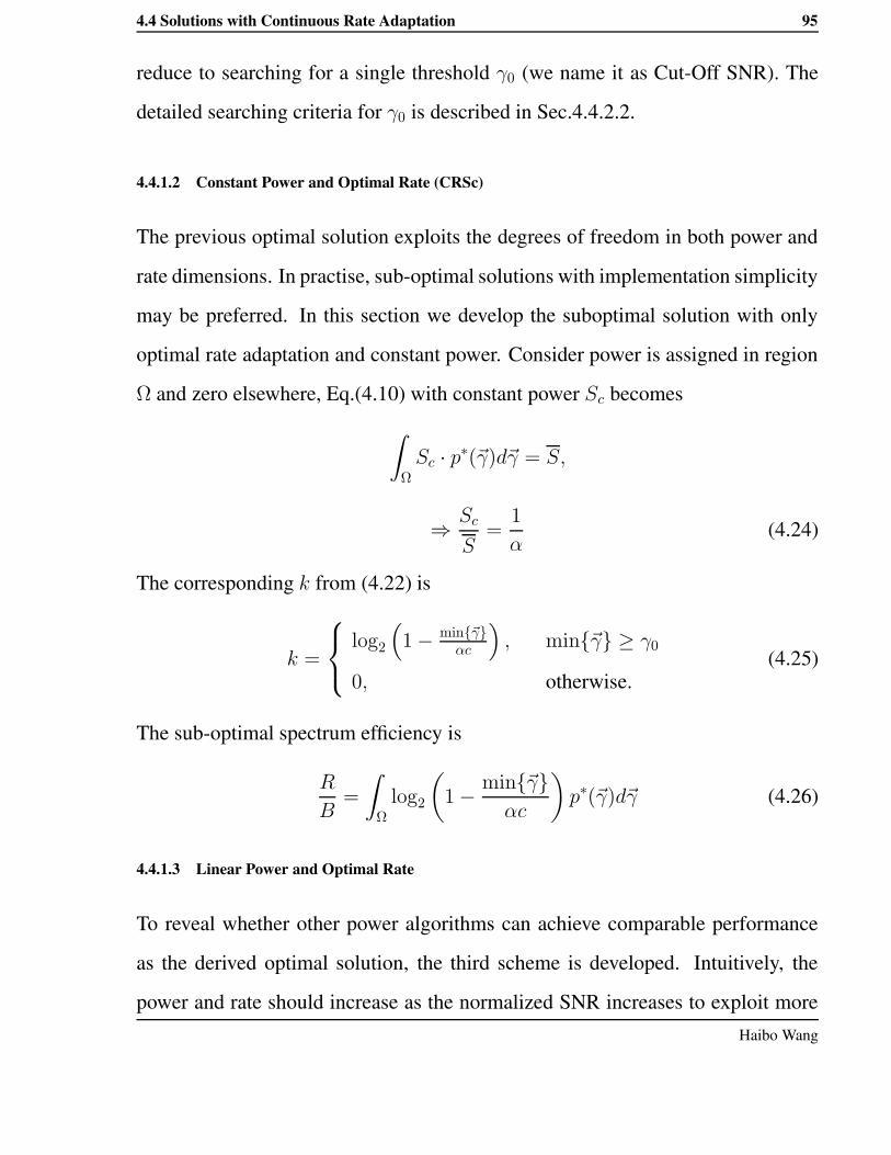
4.4 Solutions with Continuous Rate Adaptation 95
reduce to searching for a single threshold γ0 (we name it as Cut-Off SNR). The
detailed searching criteria for γ0 is described in Sec.4.4.2.2.
4.4.1.2 Constant Power and Optimal Rate (CRSc)
The previous optimal solution exploits the degrees of freedom in both power and
rate dimensions. In practise, sub-optimal solutions with implementation simplicity
may be preferred. In this section we develop the suboptimal solution with only
optimal rate adaptation and constant power. Consider power is assigned in region
Ω and zero elsewhere, Eq.(4.10) with constant power Sc becomes
∫
Ω
Sc · p∗(~γ)d~γ = S,
⇒ Sc
S=
1
α(4.24)
The corresponding k from (4.22) is
k =
log2
(
1 − min~γαc
)
, min~γ ≥ γ0
0, otherwise.(4.25)
The sub-optimal spectrum efficiency is
R
B=
∫
Ω
log2
(
1 − min~γαc
)
p∗(~γ)d~γ (4.26)
4.4.1.3 Linear Power and Optimal Rate
To reveal whether other power algorithms can achieve comparable performance
as the derived optimal solution, the third scheme is developed. Intuitively, the
power and rate should increase as the normalized SNR increases to exploit moreHaibo Wang

96 Chapter 4. Multi-Dimensional Optimization with Analytical Model
spectrum efficiency. Hence we assume power scheme SL:
SL
S= β min~γ + ϕ (4.27)
where β and ϕ are parameters to be found to maximize spectrum efficiency.
This function subject to average power constraint
∫
Ω
SL
S· p∗(~γ)d~γ = 1
→ β
∫
Ω
min~γp∗(~γ)d~γ + ϕα = 1 (4.28)
This power scheme was investigated together with rate scheme E.q (4.14) as the
third adaptation scheme in this work.
4.4.2 Numerical Result of Case Studies
We computed the numerical results for the optimal and sub-optimal forms of S, k
and R/B with N = 2 , and the Normalized SNRs following Rayleigh distribution,
such as
p(γi) =γi exp
(
− γi2
2σ2
)
σ2. (4.29)
where θ = 10−3. So far there is not a single distribution model that can describe
the overall SNR results caused by pathloss, shadowing and multi-path. Rayleigh
distribution is frequently used in link adaptation study ([1],[4]), because multipath
is the most challenging part to be coped with link adaptations.
Use Eq.4.29 in Eq.4.20 and Eq.4.19, then
α =
[
exp
(
− γ02
2σ2
)]2
Aalborg Universitet

4.4 Solutions with Continuous Rate Adaptation 97
∆ =
∫ ∞
γ0
∫ ∞
γ0
γ1γ2 exp(
−γ21+γ2
2
2σ2
)
σ4 · min(γ1, γ2)dγ1dγ2
Here, ∆ can only be computed with numerical methods. Then we numerically
search for γ0 which maximizes
R
B=
∫ ∞
γ0
∫ ∞
γ0
log2
(
c∆ − 1
αcmin(γ1, γ2)
)
·γ1γ2 exp
(
−γ21+γ2
2
2σ2
)
σ4dγ1dγ2
The resulted Sopt versus min(γ1, γ2)(dB) is plotted in Fig. 4.1, where σ = 10 cor-
responds to the average Normalized SNR γ ≈ 11dB. The optimal rate adaptation
0 5 10 15 20 25 30 35 400
0.2
0.4
0.6
0.8
1
1.2
1.4
1.6
Min SNR dB
Power schemes V.S. Group’s Mininum SNR (Rayleigh PDF, sigma=10)
SoptSc
Figure 4.1: S/S versus min~γ
scheme k versus min(γ1, γ2) under the same γ is depicted in Fig. 4.2, and the
optimal rate scheme with constant power (γ0 = 0dB) is plotted as well.Haibo Wang

98 Chapter 4. Multi-Dimensional Optimization with Analytical Model
0 5 10 15 20 25 30 35 400
2
4
6
8
10
12
14
Min SNR (dB)
K (b
its/S
ymbo
l)
Rate schemes V.S Group’s Min SNR (Rayleigh PDF, sigma=10)
Kopt, SoptKopt, Sc
Figure 4.2: k versus min~γ
4.4.2.1 Spectrum Efficiency
Numerical searching has been done to derive the optimal γ0 which maximizes
spectrum efficiencies under different γ values, since γ0 cannot be solved with
close-from expression. The derived maximum spectral efficiency are illustrated
in Fig. 4.3 for k with optimal S (the red curve) and k with constant S (the blue
dotted curve) under Rayleigh channel with N = 2. Interestingly, the spectrum
efficiency loss due to fixed power is less than 3% compared to the one with joint k
and S adaptation in the numerical results.
If we rewrite Eq.4.14 for a single user case with the SNR expression in
Eq.4.6,
k = log2
(
1 +SNR
− ln(5θ)1.6
)
.
Aalborg Universitet

4.4 Solutions with Continuous Rate Adaptation 99
10 15 20 25 301
2
3
4
5
6
7
8
9
10
Spe
ctru
m E
ffici
ency
(bps
/Hz)
Average SNR (dB)
Spectrum Efficiency per UE in Rayleigh channel
CRSopt CRScShannon capacity
Figure 4.3: Spectrum Efficiency per User in Rayleigh Channel
Comparing with Eq.4.2, it is obvious that we can assume
Υ =− ln(5θ)
1.6(4.30)
Hence the capacity gap Υ depends on the modulation scheme and the target BER,
i.e, Υ = 3.314 at θ = 10−3 for MQAM.
To compare the performance upper bound that can be derived from Shannon
capacity and the one from our approach, we rewrite Eq.4.15 as
(
R
B
)
Shannon
=
∫
(R+
0 )N
k(~γ)p∗(~γ)d~γ
=
∫
(R+
0 )N
log2
[
1 − min~γ S(~γ)
S
]
p∗(~γ),
and apply the same Lagrange method as in the CRSopt schcme. The results are
depicted as the black curve in Fig. 4.3, which reveals that the spectral efficiencyHaibo Wang

100 Chapter 4. Multi-Dimensional Optimization with Analytical Model
upper bound derived from Shannon capacity is much higher than the upper bound
MQAM signal can achieve. For example, the Shannon upper bound is higher
than our upper bound (both with CRSopt scheme) by 1.23bit/s/Hz at 10dB, and
1.72bit/s/Hz at 20dB (43.4% and 18.6% more than CRSopt). This means, the
optimal spectral efficiency analysis with our method is much more accurate than
that based on Shannon capacity.
4.4.2.2 Selection of Cut-Off SNR Value
In this subsection we describe how to select the optimal Cut-Off SNR value. The
Cut-Off SNR should both maximize the spectrum efficiency for the given adap-
tation scheme and be physically meaningful, such that S(γ0) ≥ 0, and S(γ0) ≥0 ⇒ k(γ0) ≥ 0. The relation between spectrum efficiency and the Cut-Off SNR
values in CR − Sopt solution is illustrated by the blue curve in Fig. 4.4(a), and
the maximum and minimum values of power in CRSopt scheme derived from
different Cut-Off SNRs are plotted in Fig. 4.4(b). In Fig. 4.4(a), the spectrum ef-
ficiency (SE) keeps decreasing as Cut-Off SNR increases (as in 4.4(a)), but the
loss of efficiency is negligible when γ0 ≤ 6dB. On the other hand, the minimum
power values in Fig. 4.4(b) are negative when γ0 < 3dB. Therefore the optimal
valid Cut-Off SNR should be about 3dB. Such study has been done for SNRmean
between 10dB and 25dB, and the results suggest the optimal valid Cut-Off SNR
should be between 3dB and 6dB for this SNRmean range.
For CRSc solution (the green curve in Fig. 4.4(a)), the allocated power value
is positive and constant, and the Cut-Off SNRs which leads to the maximum spec-
tral efficiency is between 4 and 6dB.
Aalborg Universitet

4.4 Solutions with Continuous Rate Adaptation 101
0 2 4 6 8 10 120
0.2
0.4
0.6
0.8
1
1.2
1.4
1.6
1.8
Cut−off SNR (dB)
Spe
ctru
m E
ffici
ency
(bps
/sym
bol)
Rayleigh PDF, mean=10dB
CRSoptCRSc
(a) Impact on per User Spectrum Efficiency
0 1 2 3 4 5 6 7 8 9 10−2
−1
0
1
2
3
4
5
6Max and Min S/Smean V.S Cut−Off SNR, Rayleigh PDF(mean=10dB)
Cut−Off SNR (dB)
S/S
mea
n
SminSmax
(b) Impact on Min and Max Power for CRSopt
Figure 4.4: Impact of Cut-Off SNR (Rayleigh PDF, Mean=10dB)
Haibo Wang

102 Chapter 4. Multi-Dimensional Optimization with Analytical Model
4.4.2.3 Linear Power and Optimal Rate
Different β and ϕ were tested to maximize the spectrum efficiency of the kopt, SL.
Due to the constraint (4.28), once β, Mean SNR and Cut-Off SNR are selected,
ϕ is decided. The value of β is also limited by S(γ0) ≥ 0. In Fig. 4.5, differ-
10−4 10−3 10−2 10−1 1001.25
1.3
1.35
1.4
1.45
1.5
1.55
1.6
1.65
beta
Spe
ctru
m E
ffici
ency
(bps
/Hz)
Spectrum Efficiency Versus beta (SNRmean=10dB)
gamma0=4dBgamma0=0dB
Figure 4.5: Linear Power Adaptation, Impact of Slope β on Spectrum Efficiency
ent Cut-Off values did not make much difference since the curve with Cut-Off at
0dB and 4dB are overlapping with each other. The maximum spectrum efficiency
in Fig. 4.5 are only 1% less than that of kopt, Sopt while β ≤ 0.05. This re-
sult shows that other options of power schemes can also achieve nearly optimal
performance, if applied together with Eq.4.14 and carefully designed parameters.
Actually in such optimum scenario of β the curve of 4.27 would be very
close to the curve of Eq.(4.24). For simplicity reason, the constant power and
optimal rate adaptation scheme would still be the best adaptation scheme.
Aalborg Universitet

4.5 Solutions with Discrete Rate Adaptation 103
4.5 Solutions with Discrete Rate Adaptation
In this section, Lagrange method is applied with discrete transmission data rate,
where k can only be chosen from a set of integer numbers kmM−1m=0 . A sub-
optimal solution with constant power is also derived.
4.5.1 Discrete Rate and Optimal Power (DRSopt)
4.5.1.1 Unicast Case
For a point-to-point channel, the rate km can be assigned when the γ falls into
a region [Γm, Γm+1) (m = 0..M − 1 and ΓM = ∞). No data is transmitted if
γ < Γ0. For such a fixed set of rate values, the optimal rate adaptation becomes to
find the optimal rate region boundaries Γm. The Lagrangian for this problem can
be set as:
J (S(γ), Γ0, Γ1, ..., ΓM)
:=M−1∑
m=0
km
∫ Γm+1
Γm
p(γ)dγ + λ
[∫
Ω
S(γ)p(γ)dγ − S
]
(4.31)
From Eq.4.12 we can derive
S(γ)
S=
F (km)
γ(4.32)
where
F (km) = c1 · (2km − 1)
and c1 = ln(5θ)−1.6 .
Haibo Wang

104 Chapter 4. Multi-Dimensional Optimization with Analytical Model
Hence the Lagrange function can be rewritten as:
J (Γ0, Γ1, ..., ΓM) :=
M−1∑
m=0
km
∫ Γm+1
Γm
p(γ)dγ
+λ
[
M−1∑
m=0
∫ Γm+1
Γm
F (km)
γp(γ)dγ − 1
]
(4.33)
By solving the following equations for Γm
∂J∂Γm
= 0, 0 ≤ m ≤ M − 1 (4.34)
we can obtain the optimal boundaries with the forms:
Γ0 = −λ · F (k0)
k0(4.35)
Γm = −λ · F (km) − F (km−1)
km − km−11 ≤ m ≤ M − 1, (4.36)
and the value of λ can be derived from the power constraint:
M−1∑
m=0
∫ Γm+1
Γm
F (km)
γp(γ)dγ − 1 = 0 (4.37)
For a Rayleigh fading channel, Eq.4.37 can be calculated as
M−1∑
m=0
F (km)
∫ Γm+1
Γm
1
γ· γ
σ2exp(− γ2
2σ2)dγ = 1 (4.38)
⇒ 1
σ
√
π
2·
M−1∑
m=0
F (km)
[
erf(Γm+1
σ√
2) − erf(
Γm
σ√
2)
]
= 1 (4.39)
Assume km = 2, 4, 6, 8 (m = 0, 1, 2, 3) for 4QAM, 16QAM,64QAM and 256QAM
under Rayleigh fading channel, and let Γ4 = inf. We can solve Eq. 4.39 to get
Aalborg Universitet
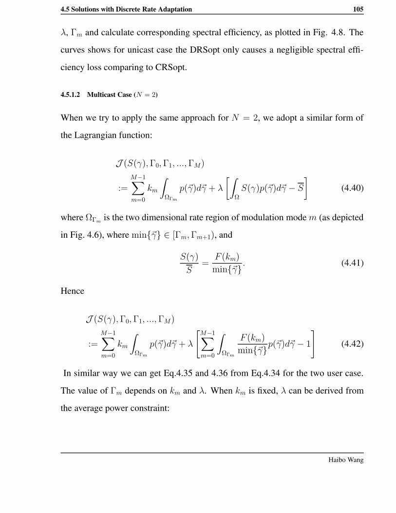
4.5 Solutions with Discrete Rate Adaptation 105
λ, Γm and calculate corresponding spectral efficiency, as plotted in Fig. 4.8. The
curves shows for unicast case the DRSopt only causes a negligible spectral effi-
ciency loss comparing to CRSopt.
4.5.1.2 Multicast Case (N = 2)
When we try to apply the same approach for N = 2, we adopt a similar form of
the Lagrangian function:
J (S(γ), Γ0, Γ1, ..., ΓM)
:=
M−1∑
m=0
km
∫
ΩΓm
p(~γ)d~γ + λ
[∫
Ω
S(γ)p(~γ)d~γ − S
]
(4.40)
where ΩΓmis the two dimensional rate region of modulation mode m (as depicted
in Fig. 4.6), where min~γ ∈ [Γm, Γm+1), and
S(γ)
S=
F (km)
min~γ . (4.41)
Hence
J (S(γ), Γ0, Γ1, ..., ΓM)
:=
M−1∑
m=0
km
∫
ΩΓm
p(~γ)d~γ + λ
[
M−1∑
m=0
∫
ΩΓm
F (km)
min~γp(~γ)d~γ − 1
]
(4.42)
In similar way we can get Eq.4.35 and 4.36 from Eq.4.34 for the two user case.
The value of Γm depends on km and λ. When km is fixed, λ can be derived from
the average power constraint:
Haibo Wang
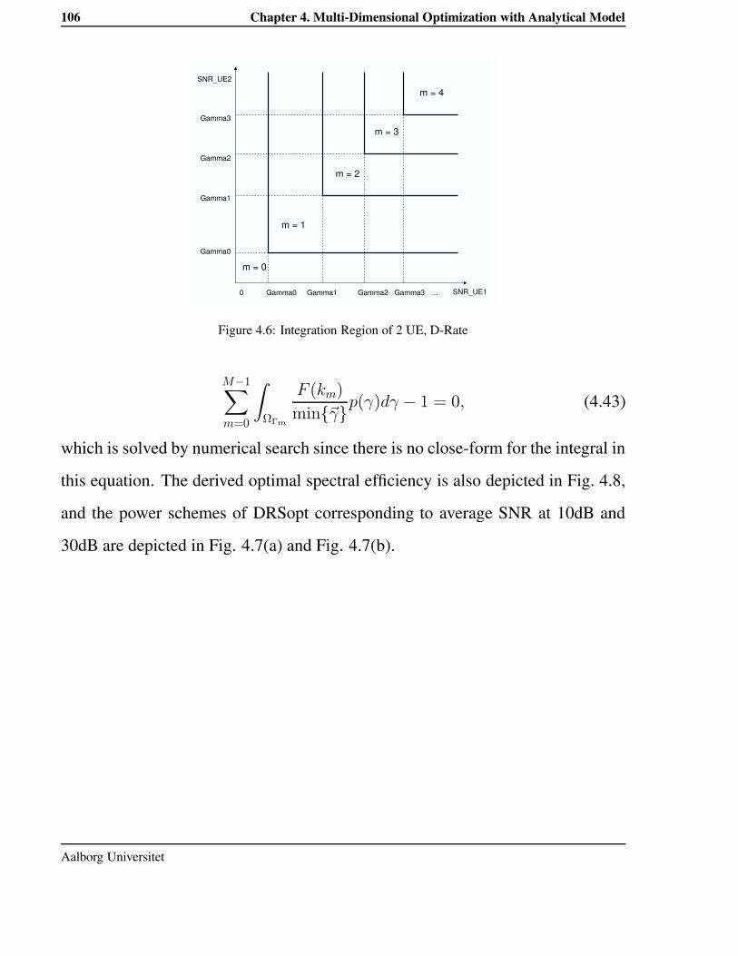
106 Chapter 4. Multi-Dimensional Optimization with Analytical Model
SNR_UE1
SNR_UE2
0 Gamma0 Gamma1 Gamma2 Gamma3 …
Gamma3
Gamma2
Gamma1
Gamma0
m = 0
m = 4
m = 1
m = 3
m = 2
Figure 4.6: Integration Region of 2 UE, D-Rate
M−1∑
m=0
∫
ΩΓm
F (km)
min~γp(γ)dγ − 1 = 0, (4.43)
which is solved by numerical search since there is no close-form for the integral in
this equation. The derived optimal spectral efficiency is also depicted in Fig. 4.8,
and the power schemes of DRSopt corresponding to average SNR at 10dB and
30dB are depicted in Fig. 4.7(a) and Fig. 4.7(b).
Aalborg Universitet
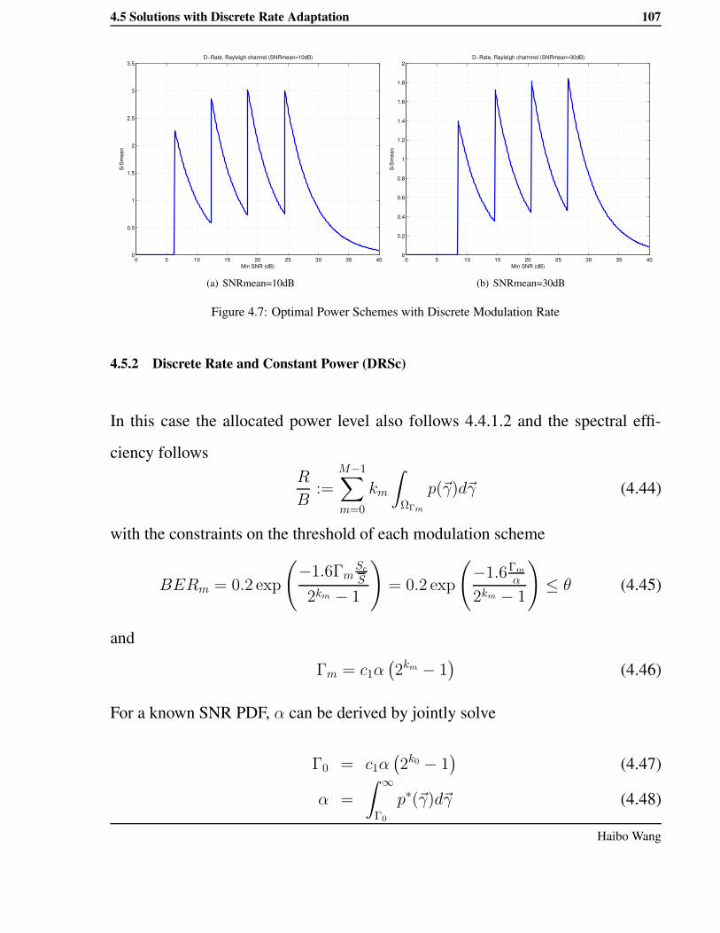
4.5 Solutions with Discrete Rate Adaptation 107
0 5 10 15 20 25 30 35 400
0.5
1
1.5
2
2.5
3
3.5
Min SNR (dB)
S/S
mea
n
D−Rate, Rayleigh channel (SNRmean=10dB)
(a) SNRmean=10dB
0 5 10 15 20 25 30 35 400
0.2
0.4
0.6
0.8
1
1.2
1.4
1.6
1.8
2
Min SNR (dB)
S/S
mea
n
D−Rate, Rayleigh channnel (SNRmean=30dB)
(b) SNRmean=30dB
Figure 4.7: Optimal Power Schemes with Discrete Modulation Rate
4.5.2 Discrete Rate and Constant Power (DRSc)
In this case the allocated power level also follows 4.4.1.2 and the spectral effi-
ciency followsR
B:=
M−1∑
m=0
km
∫
ΩΓm
p(~γ)d~γ (4.44)
with the constraints on the threshold of each modulation scheme
BERm = 0.2 exp
(
−1.6ΓmSc
S
2km − 1
)
= 0.2 exp
(
−1.6Γm
α
2km − 1
)
≤ θ (4.45)
and
Γm = c1α(
2km − 1)
(4.46)
For a known SNR PDF, α can be derived by jointly solve
Γ0 = c1α(
2k0 − 1)
(4.47)
α =
∫ ∞
Γ0
p∗(~γ)d~γ (4.48)
Haibo Wang

108 Chapter 4. Multi-Dimensional Optimization with Analytical Model
The spectral efficiency results for Rayleigh PDF, D-Rate and Constant power
scheme in unicast and multicast (N = 2) cases are illustrated in Fig. 4.8.
4.5.3 Numerical Results of Case Studies
The spectral efficiency curves of all Lagrange-based solutions are presented in
Fig. 4.8 for comparison and analysis.
10 15 20 25 300
1
2
3
4
5
6
7
8
9
Spe
ctru
m E
ffici
ency
(bps
/Hz)
Average SNR (dB)
Spectrum Efficiency per UE in Rayleigh channel
2UE, CRSopt2UE, CRSc1UE, CRSopt1UE, DRSopt2UE, DRSopt1UE, DRSc2UE, DRSc
Figure 4.8: Per User Spectral Efficiency of All Adaptation Schemes
4.5.3.1 Spectral Efficiency Loss due to Discrete Rate Adaptation
In Fig. 4.8, the performance of DRSopt is only slightly lower than that of CRSopt.
This means the optimal solution with discrete data rate and continuous power can
achieve the spectral efficiency which is very close to the upper bound provided by
the optimal one with continuous rate and power. Because continuous rate adap-
tation cannot really be implemented with practical modulation constellations, butAalborg Universitet

4.5 Solutions with Discrete Rate Adaptation 109
the exact spectral efficiency of discrete rate adaptations may change according to
the available modulation modes, the optimal spectral efficiency of CRSopt can be
considered as a general upper bound, and a very accurate estimation (comparing to
Shannon-capacity-based upper bound) for the optimal rate and power adaptation
schemes in practice.
4.5.3.2 Spectral Efficiency Loss due to Fixed Power
Unlike the continuous rate scenario, significant performance losses can be ob-
served for the DRSc scheme comparing to the DRSopt scheme in both unicast
and multicast (2 UEs). E.g, the per user spectral efficiency loss increases from
about 0.33 bps/Hz up to about 0.89 bps/Hz for the multicast group of 2 UEs as the
average SNR increases from 10dB to 30dB. This fact suggests that discrete rate
adaptation should always be applied jointly with power adaptation to maximize
the spectral efficiency.
4.5.3.3 Spectral Efficiency Loss and Gain due to Multicasting
If we compare the per user performance of the same adaptation schemes (CRSopt,
DRSopt, DRSc) under unicast and multicast as depicted in Fig. 4.8, a gap can
be observed between each pair of them . The multicast spectral efficiencies are
around 0.32 to 0.50bps/Hz less than the unicast values for the same adaptation
scheme. This performance loss is due to the fact that the instantaneous rate as-
signed to the channel is limited by the worst fading state among users in a multicast
group. And such loss is expected to increase as group size increases. However,
such spectrum efficiency has been achieved by two receivers each in multicast,Haibo Wang

110 Chapter 4. Multi-Dimensional Optimization with Analytical Model
so the total spectrum efficiency of the multicast channel has been nearly doubled
comparing to the unicast channel. This fact implies that even though the multicast
adaptation is limited by the instantaneous worst channel during each transmission
burst, it is still much more efficient to serve two users with a multicast channel
than with two unicast channels.
4.6 Conclusion and Future Work
In this work we analytically derived the spectral efficiency upper-bound of a mul-
ticast channel and the optimal joint power and rate adaptation scheme. With an
ideal assumption that the data rate can be allocated continuously, nearly optimal
spectrum efficiency can also be achieved with constant power and optimal rate
allocation. However, under a more practical setting with discrete data rate and
limited modulation modes options, joint power and rate adaptation significantly
outperforms constant power scheme. Last but not the least, the maximum average
spectrum efficiency per user of a multicast group is close enough to the unicast
case, such that the system spectrum efficiency gain can be improved dramatically.
Therefore it is always more efficient to switch to multicast mode from unicast
mode.
So far all the studies in this thesis only optimize link adaptation schemes on
bit level. However, in practice bit streams are transmitted in packets/frames, and
the performance on packet level may influence on the user perceived QoS more
significantly. That is, we extend our study to packet level adaptations, i.e., on the
data link layer, in the next chapter.
Aalborg Universitet

4.6 Conclusion and Future Work 111
Note: The works presented in this chapter have been published in [5], and will
also appear in [6].
Haibo Wang

Bibliography
[1] Q. Du and X. Zhang, “Joint Power and Constellation Size Adaptation for Mo-
bile Multicast Employing MQAM Over Wireless Fading Channels,” in Proc.
IEEE Int. Conf. on Communications 2007 (ICC 2007), Glasgow, UK, Jun.
2007.
[2] W. Ge, J. Zhang, and S. Shen, “A Cross-Layer Design Approach to Multicast
in Wireless Networks,” in Proc. IEEE Trans. Wireless Commun., vol. 6, np. 3,
Mar. 2007.
[3] H. Wang, H. P. Schwefel and T. S. Toftegaard, “History-based Adaptive Mod-
ulation for a Downlink Multicast Channel in OFDMA systems,” in Proc.
IEEE Wireless and Networking Conference (WCNC’08), Las Vegas, USA,
Mar. 2008.
[4] S. T. Chung, A. J. Goldsmith, “Degrees of Freedom in Adaptive Modulation:
A Unified View,” in IEEE Trans. Commun., vol. 49, no. 9, pp. 1561-1571,
Sept. 2001.
[5] H. Wang, H. P. Schwefel and T. S. Toftegaard, “The Optimal Joint Power112

BIBLIOGRAPHY 113
and Rate Adaptation for Mobile Multicast: A Theoretical Approach,” in Proc.
IEEE Sarnoff Symposium, Princeton, USA, Mar. 2008.
[6] H. Wang, H. P. Schwefel and T. S. Toftegaard, “Mobile Multicast: the Optimal
Power and Rate Adaptations in a Unified View,” in preparation.
Haibo Wang

Chapter 5
Cross Layer Design for Multicast
In this chapter, the reliability constraint is re-considered to include the influence
of multiple layers. We extend the cross-layer model proposed in [3] from unicast
to multicast scenario, and develop packet-combine-based multicast ARQ schemes
and related AMC schemes within this cross-layer context. The performances of
several multicast ARQ and AMC combinations, with or without cross-layer de-
sign, are analyzed with numerical results.
5.1 Motivation
In the previous chapters we have only included the reliability constraint in error
probability (i.e., BER) for wireless video applications, but have not considered the
impact of error patterns toward the quality of video transmissions. Such impact
involves both the error pattern due to wireless channel, and the process in which
the video stream is encoded on the application layer, and encapsulated into the
transmission data units on the network layer, the link layer and the physical layer.
Let us first briefly review a video-streaming transmission process.
In a video streaming transmission over wireless networks, application level114

5.1 Motivation 115
video frames (a video frame in this chapter refers to a coded single still image)
are generated from the original video streams by a video encoder, with contempo-
rary video compression and transmission standards (e.g., Moving Picture Experts
Group (MPEG) -2, MPEG-4 and H.264). In these standards, some frames are
reused for motion-compensated prediction [1] so that many repeated parts among
consecutive images need not to be transmitted in each coded frame, which effi-
ciently compress the data volume of the generated frames. As a consequence, the
coded video contents are correlated on frame level. Then the coded video frames
are passed through the network layer, i.e, encapsulated in IP packets. On the link
layer, the video in IP packets need to be segmented into Packet Data Unit (PDU)
to be delivered to the physical layer,. The segmentation is necessary since Layer
2 (L2) PDU is usually smaller than the IP packets, for the ease of correct transmis-
sion in wireless mobile channels (In the rest of this chapter, the term packet will
refer to a L2 PDU only, since the network layer study is out of our scope.). In the
physical layer transmissions, the wireless channels may introduce burst of errors
so that a whole L2 packet is dropped. Unlike distributed bit errors, such burst
errors are hard to be recovered by error correction codes no matter with physical
layer FEC or with application layer FEC. On the application layer, these errors
will propagate to following video frames and seriously degrade the video quality.
Hence we consider that the instantaneous L2 Packet Error Ratio (PER) is crucial
for the user perceived QoS, and start improving spectral efficiency on the data link
layer with this PER constraint.
As the previous chapters revealed, when the error constraint (i.e, BER) is
instantaneous, the transmitter has to adapt to the worst link receiver in the group.Haibo Wang

116 Chapter 5. Cross Layer Design for Multicast
If this instantaneous constraint can be relaxed, more spectral efficiency may be
exploited in the efficiency-reliability tradeoff. From a cross-layer perspective, in a
system with L2 ARQ, the instantaneous PER constraint can be seen as the residual
PER after retransmission, and the PER limit for the first transmission may be
relaxed if the physical layer and data link layer can be jointly designed.
The main problem when applying ARQ to Multicast is scalability [2]. As-
sume the channel fading of all users are i.i.d, and the average packet loss ratio is P .
If in a unicast link the probability that a packet is lost and requires retransmissions
is P , in a multicast link with N users, the probability to request retransmission
for a multicast packet is 1 − (1 − P )N , since any of N users lost this packet
would trigger a retransmission. When N is large, retransmission will be requested
frequently, which will cost lots of transmission capacity and reduce the overall
spectral efficiency. However, if several retransmission packets can be combined,
such scalability problem may be solved.
Motivated by these considerations, we adopt the cross-layer design frame-
work from [3], and jointly optimize the AMC schemes and ARQ scheme for wire-
less multicast. Multiple cross-layer designed AMC-ARQ strategies are proposed
and compared with other strategies, e.g., AMC without ARQ strategies and AMC-
ARQ strategies without cross-layer design. We also develop a packet-combine-
based ARQ to solve the scalability problem.
5.2 Related Work
ARQ with packet combining has been proposed by some researchers. The au-
thors of [4] had proposed to use XOR operation among retransmitted packets forAalborg Universitet

5.2 Related Work 117
multiple unicast links. In their solution, each receiver has to overhear the packets
transmitted to other users and store them. The transmitter will put multiple lost
packets of different receivers into one Combined Packet (CP) with ’XOR’ oper-
ation, and resend such a CP. Then each receiver expecting its retransmission can
extract its own retransmitted packet utilizing its stored correct packets of other re-
ceivers. However, the price of this scheme in multi-user unicast case is that each
receiver consumes N times the power as if it had only received its own packet.
When there are N unicast receivers in a cell, the power consumption of each one
will be N times larger than without this packet XOR.
This drawback does not exist in multicast case. E.g, if there is a 1/N outage
ratio within N receivers for a given transmission rate according to their mean SNR,
and let D(k) represent the kth multicast data packet. During N transmission bursts
each receiver got N − 1 packets correctly, and failed to receive one out of N
packets. They send their requests via an error-free feedback channel, and the
transmitter resends the D(N+1) = D(1)⊕
D(2)⊕
...⊕
D(N) afterward. Each
receiver will be able to extract its intended packet from D(N + 1) and all its
previously received and stored N − 1 packets.
More systematical packet combining methods are the packet level Reed-
Solomon coding. A group of K consecutive packets are feed into a packet-based
encoder to generate L − K parity packets, and the L output packets, including
K original packets and L − K redundant packets, are sent along on the chan-
nel as a Transmission Group (TG). Three HARQ schemes based on packet level
Reed-Solomon codes were designed in [5] for UMTS downlink multicast chan-
nel, and the authors conclude that which design is better rather depends on theHaibo Wang

118 Chapter 5. Cross Layer Design for Multicast
multicast channel error process in reality (e.g, independent error model or burst
error model). The authors of [6] further proposed two more HARQ schemes as
the extensions of scheme A2 and A3 in [5] and achieve a certain improvement
in throughput and mean Service Data Unit delay, especially when the multicast
group size is large.
A cross-layer design was proposed in [3] for unicast links, which combined
AMC and HARQ. In the spectral efficiency results of this work, the cross-layer
scheme with one retransmission outperforms AMC without ARQ scheme by about
0.25 bits/symbol. However, further increase of maximum allowed retransmissions
only results in diminishing gain. This work implies that one retransmission should
be sufficient in joint AMC and ARQ design if the optimization target is to improve
spectral efficiency while a residual packet loss ratio is allowed. This work inspired
our proposals in its cross-layer framework.
Aalborg Universitet

5.3 Cross-Layer System Model 119
5.3 Cross-Layer System Model
A wireless transmitter in contemporary systems (e.g, UMTS HSDPA, IEEE 802.11
a, b and g ) usually has both Adaptive Modulation and Coding (AMC) and ARQ
functionalities. Hence we assume the transmitter includes both functions, which
are aware of each other. We also assume constant power transmission to reduce the
design complexity in the cross-layer framework. Assume a base station multicas-
ting to a group of N mobile receivers, where the Layer-1 (L1) feedback channels
can provide instantaneous and perfect CSIs from the receivers to the BS transmit-
ter, and the packet level, Layer-2 (L2) feedbacks will be also errorfree. The cross-
layer system model between the transmitter and one of the receiver is illustrated
in Fig. 5.1. The channels are assumed as frequency-flat block fading channels,
hence the SINR, noted as γi(i = 1..N), will not change during the transmission
time of a PDU. The PDFs of γi follow Independent Identical Distributions (i.i.d),
noted as p(γi). The random vector ~γ := (γ1, γ2, ..., γN) represents a fading state
of the Multicast group, with probability density function p∗(~γ) =∏N
i=1 p(γi). The
transmitted data block includes both error detection (ED) coding CRC and forward
error correction (FEC) coding.
At the physical layer, we assume the available modulation and FEC code
combinations (referred as AMC modes) are as in HIPERLAN/2. Based on the
CSI reported from all multicast receivers and the link adaptation strategy, the AMC
selector at the transmitter determines the AMC mode. At the data link layer, dif-
ferent ARQ protocols are implemented. A packet from the input buffer is sent
to the physical layer and a copy of it is also stored in the ARQ buffer as shown
in Fig. 5.1. If an error is detected in a packet, a retransmission request is sentHaibo Wang

120 Chapter 5. Cross Layer Design for Multicast
RF
AMC
ARQ
RF
ARQ
AMC
Input Buffer Output Buffer
CSI Feedback
Fading Channel
Physical Layer
Data Link Layer
Physical Layer
Data Link Layer
AMC mode
ARQ Request
Transmitter Receiver i of Multicast group
Figure 5.1: Multicast System Model with Cross-Layer Design
to the ARQ controller at the transmitter via a feedback channel; otherwise, no
retransmission request is sent. The ARQ controller at the transmitter arranges re-
transmission of the requested packet that is stored in the buffer. If a certain packet
is not requested to be resent for any of the receivers, it will be removed from the
retransmission buffer; if it is requested by all the receivers, it will be pushed down
from the ARQ buffer to the physical layer for retransmission immediately; if it is
requested by some of the receivers, the operation will depend on the investigated
ARQ schemes.
The optimization target is to maximize packet level spectral efficiency given
the following constraints:
1. Constraint 1: Maximum allowed number of retransmissions T maxr . Tmax
r is
set to 1, since the results in [3] shows that the spectral efficiency gain from
cross-layer designed ARQ diminishes as retransmission time increases.Aalborg Universitet

5.3 Cross-Layer System Model 121
2. Constraint 2: The residual packet loss ratio bound after T maxr retransmissions,
Ploss = 10−2.
On packet level, exact close-form PERs of coded modulation versus γ are not
available, but an approximation is provided in [3] as
PERm(γ) ≈
am exp(−gmγ), if γ ≥ Γm
1, if 0 ≤ γ < Γm
(5.1)
where m refer to AMC mode index, γ is the SINR of a receiver, am, gm are pa-
rameters depend on AMC mode, which are presented in Table. 5.1. Γm is the
threshold of AMC mode m. I.e., in a point-to-point link, mode m is chosen when
γ ∈ [Γm, Γm+1). The value of Γm can be varied according to the target packet
loss ratio, and the channel SINR distributions. If we only consider point-to-point
Mode 1 Mode 2 Mode 3 Mode 4 Mode 5 Mode 6Modulation BPSK QPSK QPSK 16-QAM 16-QAM 64-QAMCoding Rate 1/2 1/2 3/4 9/16 3/4 3/4Rate(bits/symbol)
0.5 1.0 1.5 2.25 3.0 4.5
am 274.7229 90.2514 67.6181 50.1222 53.3987 35.3508gm 7.9932 3.4998 1.6883 0.6644 0.3756 0.0900
Table 5.1: Transmission AMC Modes with Convolutional-Coded Modulation
transmission without ARQ, the AMC threshold can be derived from 5.1 as
Γm =1
gmln
(
am
Ploss
)
(5.2)
where Ploss is the PER constraint. Given ARQ exist, if the expected average packet
loss ratio per transmission is P0, and let PERT maxr +1 represent the residual PER
after Tmaxr + 1 transmissions for a specific packet (one orginal transmission and
Haibo Wang

122 Chapter 5. Cross Layer Design for Multicast
Tmaxr retransmissions), there must be
PERT maxr
+1 = PT max
r +10 ≤ Ploss. (5.3)
In this case the thresholds can be rewritten as
Γ′m =
1
gmln
(
am
P0
)
(5.4)
Since 0 < P0 < 1, 0 < Ploss < 1 and P0 > Ploss ⇒ Γ′m < Γm, higher data rates
can be allocated under thresholds Γ′m than under Γm. However, the retransmis-
sion will also reduce the spectral efficiency due to the parity packet transmission.
Whether such SINR threshold relaxation leads to higher spectral efficiency in total
will depend on the comparison of
Se(1) =
M∑
m=1
RmPr(m) (5.5)
and
Se(Tmaxr + 1) =
1
T
M∑
m=1
RmP ′r(m). (5.6)
where Se(1) is the spectral efficiency without retransmission, Se(T maxr +1) is the
one with at most Tmaxr retransmission. Rm is the bit per symbol in each AMC
mode, Pr(m) and P ′r(m) are the cumulated probability of SINR staying in rate
region m, and they are different due to the different rate region thresholds as in 5.2
and 5.4. T is the expected transmissions per packet,
T = 1 + P0 + P 20 + ... + P
T maxr
0 =1 − P
T maxr
+10
1 − P0(5.7)
If, for a given SINR distribution, Se(T maxr + 1) > Se(1), then we gain spectral
Aalborg Universitet

5.4 Multicast ARQ with Packet-Combining 123
efficiency with cross layer AMC at the price of packet delay.
5.4 Multicast ARQ with Packet-Combining
We analyze our multicast ARQ design in a two phase setting, the original data
transmission phase and the retransmission phase, namely the first phase and the
second phase. These two phases are considered separately for the ease of analysis,
even though they will be fulfilled alternatively and partially overlap each other in
practice. In the first phase, a large number of data packets are transmitted, such
that the packets number is enough for probabilistic analysis. The packet loss of
each user in the first phase will be reported to the transmitter. In the second phase,
the transmitter will select the most efficient way to combine the lost packets wit
XOR operation in the ARQ buffer and resend them. Under design constraint 1,
each data packet lost in the first phase will only be retransmitted once in the second
phase, thus constraint 2 and Eq.5.3 lead to
P0 =√
Ploss = 0.1 (5.8)
in which Ploss is the target residual PER and P0 is the instantaneous PER con-
straint.
In the rest of this section two cases of packet combining are discussed, a
simple case with only two users in a group, and the general case for a group with
N users (N ≥ 2).
Haibo Wang

124 Chapter 5. Cross Layer Design for Multicast
5.4.1 Two Users Group
In a group with only two receivers, a packet loss pattern in the first phase is illus-
trated in Fig. 5.2. For data packets D2, D4, D5, D10 which are only lost by one
user each, the BS can combine the retransmission, e.g. CP1 = D2
⊕
D4 (CP
stands for Combined Packet), CP2 = D5
⊕
D10, and both users can decode them
using its previously correctly received packet (e.g, UE1 use D2
⊕
CP1 = D4 and
UE2 use D4
⊕
CP1 = D2). In this case, we call the packets which can be com-
bined into one CP as match packet to each other, e.g, D2 and D4, D5 and D10. For
1 112 3 4 5 6 7 8 9 10… …
Packet stream
UE1
1 112 3 4 5 6 7 8 9 10… …UE2
Figure 5.2: Multicast Packet Loss Pattern for 2 UEs
D7, both users lost it and it cannot be combined with other lost data packets in the
retransmission, otherwise there will be at least one user who cannot decode it.
For any arbitrary packet , define L as the number of users who lost it. To
calculate the transmission per packet T when packet combination is adopted, de-
fine
η = 1/(Number of data packets included in 1 CP)
and T = 1 + η. E.g. η(D2) = η(D4) = η(D5) = η(D10) = 1/2 for packets
D2, D4, D5, D10 and T = 1 + 12
for each of them. Hence it has to be retransmitted
by itself and η(D7) = 1.
From the example in Fig. 5.2, we can derive the expected number of retrans-
missions and probabilities. That is, three are three cases for a multicast group with
N = 2:Aalborg Universitet

5.4 Multicast ARQ with Packet-Combining 125
• If no user lost this packet, no retransmission is necessary:
Pr(L = 0) = (1 − P )2,
η(L = 0) = 0;
• If one user lost this packet, packet combination with a pacet lost by the other
user can be performed:
Pr(L = 1) =
(
2
1
)
P (1 − P ),
η(L = 1) = 12 ;
• If both users lost this packet, no packet combination is possible:
Pr(L = 2) = P 2,
η(L = 2) = 1.
And the expectation of the effective transmission time for any arbitrary packet is
E[T ] = 1 +2∑
i=0
η(L = i)Pr(L = i)
= 1 + P (5.9)
5.4.2 N Users Group
Now we generalize such analysis to the N user case (N ≥ 2). There are two
lemmas for the general case:
• Lemma 1: For any arbitrary packet Dj (j is the packet index), its match
packet(s) exist iff 1 ≤ L(Dj) ≤ N − 1, and its match packet(s) are not
unique.
• Lemma 2: A CP can be made up of a subset of lost packets Dj1, ..., Djk, ...,,
(1 ≤ L(Djk) ≤ N − 1)
Haibo Wang
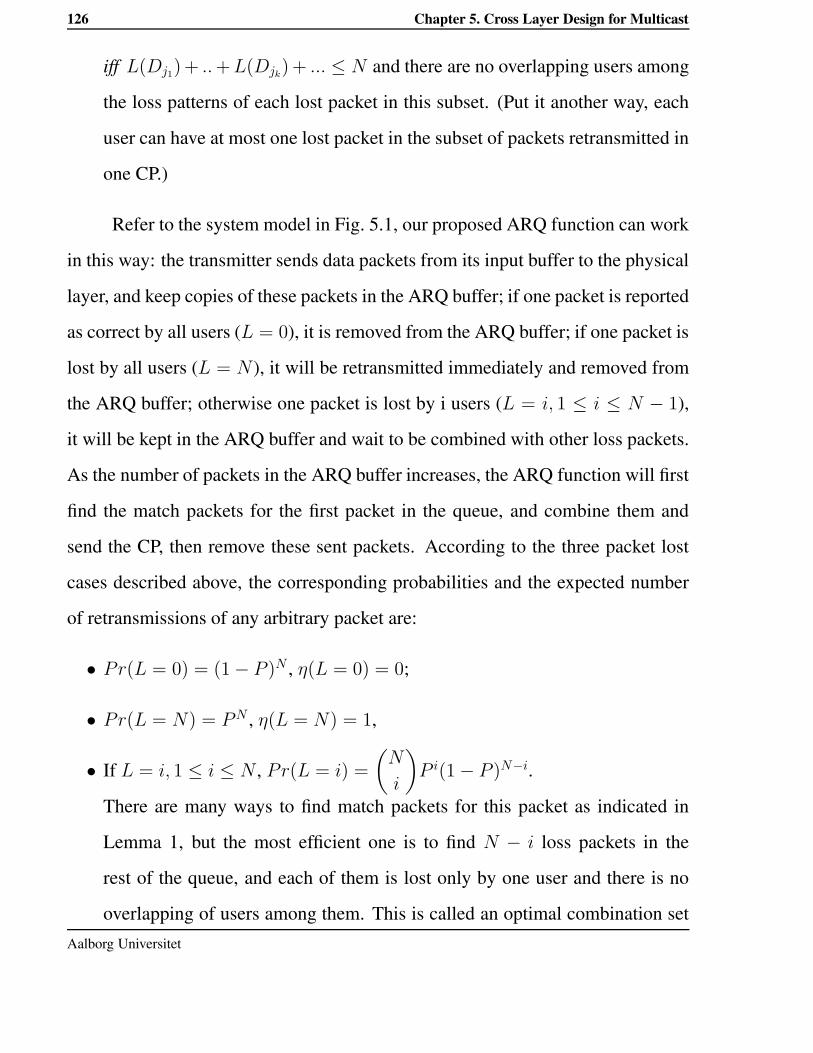
126 Chapter 5. Cross Layer Design for Multicast
iff L(Dj1) + .. + L(Djk) + ... ≤ N and there are no overlapping users among
the loss patterns of each lost packet in this subset. (Put it another way, each
user can have at most one lost packet in the subset of packets retransmitted in
one CP.)
Refer to the system model in Fig. 5.1, our proposed ARQ function can work
in this way: the transmitter sends data packets from its input buffer to the physical
layer, and keep copies of these packets in the ARQ buffer; if one packet is reported
as correct by all users (L = 0), it is removed from the ARQ buffer; if one packet is
lost by all users (L = N ), it will be retransmitted immediately and removed from
the ARQ buffer; otherwise one packet is lost by i users (L = i, 1 ≤ i ≤ N − 1),
it will be kept in the ARQ buffer and wait to be combined with other loss packets.
As the number of packets in the ARQ buffer increases, the ARQ function will first
find the match packets for the first packet in the queue, and combine them and
send the CP, then remove these sent packets. According to the three packet lost
cases described above, the corresponding probabilities and the expected number
of retransmissions of any arbitrary packet are:
• Pr(L = 0) = (1 − P )N , η(L = 0) = 0;
• Pr(L = N) = PN , η(L = N) = 1,
• If L = i, 1 ≤ i ≤ N , Pr(L = i) =
(
N
i
)
P i(1 − P )N−i.
There are many ways to find match packets for this packet as indicated in
Lemma 1, but the most efficient one is to find N − i loss packets in the
rest of the queue, and each of them is lost only by one user and there is no
overlapping of users among them. This is called an optimal combination setAalborg Universitet

5.5 AMC Strategies 127
where η(L = i) = 1N−i+1, and
E[T ]opt = 1 +N∑
i=0
η(L = i)Pr(L = i)
= 1 +
N∑
i=1
1
N − i + 1
(
N
i
)
P i(1 − P )N−i (5.10)
However, it may take very long time to cumulate all N − i + 1 match packets
for the optimal combination. Hence we also propose a suboptimal combina-
tion scheme, such that the current packet with L = i only need to be combined
with another packet with L = j, i + j ≤ N and there is no overlapping users
between the two packets, and η(L = i) = η(L = j) = 12 ,
E[T ]SubOpt = 1 + PN +1
2
N−1∑
i=1
(
N
i
)
P i(1 − P )N−i (5.11)
Note: when N = 2, the optimal and sub-optimal combination become the same.
5.5 AMC Strategies
When ARQ is not adopted in the system, the rate adaptation is limited by the
minimum received SINR among all multicast receivers, namely the Minimum-
SINR AMC strategy. With the help of ARQ, the instantaneous PER constraint of
the worst-channel receiver can be temporarily violated such that AMC strategies
other than the Minimum-SINR strategy can also be adopted. And the lost pack-
ets of the worst-channel receiver can be retransmitted such that its residual PER
may still be within Ploss. The AMC strategies we investigate jointly with ARQ are:
Haibo Wang

128 Chapter 5. Cross Layer Design for Multicast
1. Minimum SINR AMC
In this strategy the data rate has to satisfy the instantaneous PER constraint
of the worst SINR receiver, such as
AMC mode m is chosen if min~γ ∈ [Γm, Γm+1)
2. Second Minimum SINR AMC
In this strategy the data rate has to satisfy the instantaneous PER constraint
of the second least SINR receiver, noted as γMin2, i.e.,
AMC mode m is chosen if γMin2 ∈ [Γm, Γm+1)
3. Average PER-based AMC
In this strategy the data rate is chosen such that the corresponding average
instantaneous PER among group members is the closest to the PER constraint
of all rate options. Before each transmission burst is sent,For AMC mode m = 1..M,
PERm =∑N
i=1 PERm(γi)
mopt = arg min |PERm − P0|
Assign mopt.
Since strategy 2 and 3 do not guarantee the instantaneous PER of each receiver
during the first transmission, the residual PER of a packet has to be guaranteed by
the ARQ schemes.Aalborg Universitet
5.6 Evaluation Methods 129
5.6 Evaluation Methods
In total, there are three adaptation strategies to be compared in this chapter.
• The proposed cross layer approach, where the instantaneous PER relaxation
due to ARQ is adopted, so
P0 =√
Ploss = 0.1
• Layered multicast AMC and ARQ. In this case multicast AMC and ARQ
functions both exist in the system, but they are not jointly designed. I.e, the
AMC thresholds are derived from
P0 = Ploss = 0.01;
• AMC alone.
The AMC strategy 1 can be applied with or without ARQ, with or without cross-
layer design, since it uses an absolute instantaneous PER constraint in AMC mode
selection for the first transmission. E.g., the target residual PER is 0.01, hence
the PER constraint without ARQ is 0.01; it is also 0.01 with ARQ but no X-layer
design, since then AMC part is not aware the exist of ARQ; it is relaxed to 0.1
with ARQ and cross-layer awareness. But AMC strategy 2 and 3 must be applied
with ARQ, as explained in Sec. 5.5.
On the other hand, three different ARQ schemes are to be compared:
• Optimal packet combining
• Sub-optimal packet combiningHaibo Wang

130 Chapter 5. Cross Layer Design for Multicast
• Plain ARQ, no packet combining
5.7 Case Study I: N = 2
In this case study, a group of 2 users under i.i.d Rayleigh fading channels is con-
sidered. The attempt is to derive the close-form solution of the spectral efficien-
cies for two AMC strategies, strategy 1 and 2, with or without cross-layer design.
Strategy 3 is not studied since it is difficult to build a close-form model for its
algorithm. So there are four AMC-ARQ strategies to be evaluated:
• Strategy S1: Minimum SINR AMC, with the packet-combining ARQ and
cross-layer design.
• Strategy S2: Maximum SINR AMC, with the packet-combining ARQ and
cross-layer design. In a two users group, the strategy 2 of Sec. 5.5 reduces
to this Maximum SINR AMC. Also, this scheme cannot be adopted without
ARQ.
• Strategy S3: Minimum SINR AMC, without ARQ.
• Strategy S4: Minimum SINR AMC, with ARQ but not cross-layer design.
As explained in Sec. 5.4.2, the optimal and sub-optimal packet-combining ARQ
are the same at N = 2.
5.7.1 Performance Analysis in Close-Form Expression
According to Eq.5.5, the per user spectral efficiency from the first transmission is
Se(1) =
M∑
m=1
Rm
∫ ∫
Ωm
p(γ1, γ2)dγ1 (5.12)
Aalborg Universitet

5.7 Case Study I: N = 2 131
where the rate region Ωm corresponding to rate Rm is a two-dimensional area
depending on the rate adaptation strategy, and p is the joint PDF of γ1 and γ2.
Assume only one combined retransmission is allowed for any loss packet,
hence the per user spectral efficiency after the retransmission is
Se(Tmaxr + 1) =
Se(1)
T. (5.13)
For the ease of presenting different AMC strategies in the integrals, let γd
represent the dominant SINR for rate selection, hence
• Min-SINR AMC, γd = γmin := minγ1, γ2;
• Max-SINR AMC, γd = γmax := maxγ1, γ2.
On average, the expected transmission time per packet with loss probability P
among users are T = 1 + P , where
P = PER1 = PER2
=
∑Mm=1 Rm
∫ ∫
Ωm
PERm(γ1)p(γ1, γ2)dγ1dγ2
Se(1), (5.14)
in which PERm(γ1) can also be PERm(γ2) given the users’ SINR PDFs are i.i.d.
According to Eq. 5.9, Eq.5.13 and 5.14, the expected per user spectral efficiency
is
Se(Tmaxr + 1) =
Se(1)
1 + 1Se(1)
∑Mm=1 Rm
∫ ∫
Ωm
PERm(γ1)p(γ1, γ2)dγ1dγ2
(5.15)
Haibo Wang

132 Chapter 5. Cross Layer Design for Multicast
To observe the system performance, it is necessary to derive Se(1), P and
Se(Tmaxr + 1). Hence we have to solve the integral of PERm and the integral of
p(γ1, γ2) in rate region Ωm, and the shape of Ωm depends on the AMC strategy.
5.7.1.1 Close-Form Solution for Min-SINR AMC
Starting with AMC strategy 1, the rate regions will have the shapes as in Fig. 5.3,
and the integration of PERm in such rate regions can be calculated as
SINR_UE1
SINR_UE2
0 Gamma0 Gamma1 Gamma2 Gamma3 …
Gamma3
Gamma2
Gamma1
Gamma0
m = 0
m = 4
m = 1
m = 3
m = 2
Figure 5.3: Integration Region of 2 UEs, D-Rate
Aalborg Universitet
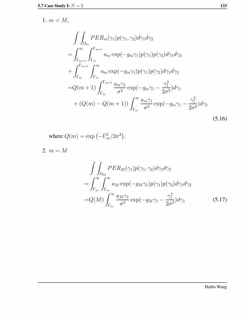
5.7 Case Study I: N = 2 133
1. m < M ,
∫ ∫
Ωm
PERm(γ1)p(γ1, γ2)dγ1dγ2
=
∫ ∞
Γm+1
∫ Γm+1
Γm
am exp(−gmγ1)p(γ1)p(γ2)dγ1dγ2
+
∫ Γm+1
Γm
∫ ∞
Γm
am exp(−gmγ1)p(γ1)p(γ2)dγ1dγ2
=Q(m + 1)
∫ Γm+1
Γm
amγ1
σ2exp(−gmγ1 −
γ21
2σ2)dγ1
+ (Q(m) − Q(m + 1))
∫ ∞
Γm
amγ1
σ2exp(−gmγ1 −
γ21
2σ2)dγ1
(5.16)
where Q(m) = exp(
−Γ2m/2σ2
)
.
2. m = M
∫ ∫
ΩM
PERM(γ1)p(γ1, γ2)dγ1dγ2
=
∫ ∞
Γm
∫ ∞
Γm
aM exp(−gMγ1)p(γ1)p(γ2)dγ1dγ2
=Q(M)
∫ ∞
Γm
aMγ1
σ2exp(−gMγ1 −
γ21
2σ2)dγ1 (5.17)
Haibo Wang

134 Chapter 5. Cross Layer Design for Multicast
5.7.1.2 Close-Form Solution for Max-SINR AMC (Second-Min-SINR AMC @ N=2)
For AMC strategy 2, rate region Ωm is represented in Fig. 5.4. The integration of
SINR_UE1
SINR_UE2
0 Gamma0 Gamma1 Gamma2 Gamma3 …
Gamma3
Gamma2
Gamma1
Gamma0
m = 0
m = 4 …
m = 1
m = 3
m = 2
Figure 5.4: Rate Regions of Max-SINR Strategy
PERm in such rate regions can be calculated as
1. m < M ,
∫ ∫
Ωm
PERm(γ1)p(γ1, γ2)dγ1dγ2
=
∫ Γm+1
0
∫ Γm+1
Γm
am exp(−gmγ1)p(γ1)p(γ2)dγ1dγ2
+
∫ Γm+1
Γm
∫ Γm
0
1 · p(γ1)p(γ2)dγ1dγ2
=(1 − Q(m + 1))
∫ Γm+1
Γm
amγ1
σ2exp(−gmγ1 −
γ21
2σ2)dγ1
+(Q(m) − Q(m + 1))(1− Q(m)) (5.18)
where Q(m) = exp(
−Γ2m/2σ2
)
.Aalborg Universitet

5.7 Case Study I: N = 2 135
2. m = M
∫ ∫
ΩM
PERM(γ1)p(γ1, γ2)dγ1dγ2
=
∫ ∞
0
∫ ∞
ΓM
aM exp(−gMγ1)p(γ1)p(γ2)dγ1dγ2
+
∫ ∞
ΓM
∫ ΓM
0
1 · p(γ1)p(γ2)dγ1dγ2
=
∫ ∞
ΓM
aMγ1
σ2exp(−gMγ1 −
γ21
2σ2)dγ1 + Q(M)(1 − Q(M)) (5.19)
So far, the integrals of PERms can be calculated, and the calculation of∑M
m=1 Rm
∫ ∫
Ωm
p(γ1, γ2)dγ1dγ2 can be done in the similar way. That is, the val-
ues of P in Eq.5.14 and Se(T maxr + 1) in Eq.5.15 can be derived accordingly.
5.7.2 Numerical Results
The resulted performances and behaviors of all four strategies are plotted in Fig. 5.5.
From Fig. 5.5(a) it can be observed that the Max-SINR strategy(strategy S2) has
the highest spectral efficiency for the first transmission with significant gain over
the other three strategies. Strategy S1 outperforms strategy S3 and S4, and the
curves of S3 and S4 are overlapping with each other. This is because S3 and
S4 follow the most strict instantaneous PER constraints, while S2 allocates data
rate more aggressively than S1. On the other hand, such aggressive adaptation
of Max-SINR resulted in a very high PER even when the average SINR is good,
while the PERs of the other two decreased fast as average SINR increase, as shown
in Fig. 5.5(b). The overall spectral efficiency results in Fig. 5.5(c) are:
when the average SINR is less than 12dB, strategy S2 performs the best,
since the rate allocation gain overcomes the efficiency loss of retransmission. TheHaibo Wang

136 Chapter 5. Cross Layer Design for Multicast
0 5 10 15 20 25 300
0.5
1
1.5
2
2.5
3
3.5
4
4.5
Mean SINR (dB)
Spe
ctra
l effi
cien
cy o
f the
firs
t tra
nsm
issi
on (b
ps/H
z)
Performances with i.i.d Rayleigh SINR, PLoss
=0.01
Min−SINR + ARQMax−SINR + ARQMin−SINR, w/o ARQMin−SINR, w/o cross−layer
(a) Spectral Efficiency of the First Transmission
0 5 10 15 20 25 3010−5
10−4
10−3
10−2
10−1
100
Mean SINR (dB)
Pac
ket e
rror
rate
of t
he fi
rst t
rans
mis
sion
Performances with i.i.d Rayleigh SINR, PLoss
=0.01
Min−SINR + ARQMax−SINR + ARQMin−SINR, w/o ARQMin−SINR, w/o cross−layer
(b) Packet Error Ratio
0 5 10 15 20 25 300
0.5
1
1.5
2
2.5
3
3.5
4
4.5
Mean SINR (dB)
Spe
ctra
l effi
cien
cy (b
ps/H
z)
Performances with i.i.d Rayleigh SINR, PLoss
=0.01
Min−SINR + ARQMax−SINR + ARQMin−SINR, w/o ARQMin−SINR, w/o cross−layer
(c) Overall Spectral Efficiency
0 5 10 15 20 25 3010−10
10−9
10−8
10−7
10−6
10−5
10−4
10−3
10−2
10−1
100
Mean SINR (dB)
Res
idua
l pac
ket e
rror
ratio
Performances with i.i.d Rayleigh SINR, PLoss
=0.01
Min−SINR + ARQMax−SINR + ARQMin−SINR, w/o ARQMin−SINR, w/o cross−layer
(d) Residual Packet Error Ratio
Figure 5.5: Performances of Different Adaptation Strategies, N = 2
Aalborg Universitet

5.8 Case Study II: N ≥ 2 137
spectral efficiency gain of strategy S2 can achieve at most 0.4bit/s/Hz in this re-
gion. As average SINR gets higher than 12dB, the performance of S1 exceeds S2,
but the difference is quite small. As the average SINR approaches 30dB, the three
curves converge. This is due to the finite modulation and coding schemes avail-
able (i.e, the adopted 6 modulation and coding combinations). When the SINR is
so high, the packet loss is small enough such that the spectral efficiency is only
limited by the highest modulation and coding rate.
However, the residual PER curves in Fig. 5.5(d) shows that strategy S2 fails
to keep the PER constraint (Ploss = 10−2) when the average SINR is less than
23dB. That is, strategy S1 is the best one for the two user group case.
5.8 Case Study II: N ≥ 2
In this section, Monte-Carlo method is adopted in numerical integrations to derive
the performances for different AMC-ARQ strategies when the multicast group
size N ≥ 2. This choice is due to two reasons: first, it is difficult to express more
complex AMC strategies such as the strategy 3 in Sec. 5.5 in close-form; second,
when N > 2, it is difficult to solve the integral along rate region Ωm in close-form,
since the shape of Ωm becomes complex as N is large. When the complexity of
deriving close-form solution is avoid, it is possible to investigate the behavior of
more AMC and ARQ combinations, as the group size increases.
Here we compared the performance of 5 different schemes in total:
• Strategy S1: Average PER AMC as the AMC strategy 3 in Sec. 5.5, with
ARQ and cross-layer design, P0 =√
Ploss = 0.1.Haibo Wang

138 Chapter 5. Cross Layer Design for Multicast
• Strategy S2: Minimum SINR AMC as the AMC strategy 1 in Sec. 5.5, with
ARQ and cross-layer design, P0 =√
Ploss = 0.1.
• Strategy S3: Second minimum SINR AMC as the AMC strategy 2 in Sec. 5.5,
with ARQ and cross-layer design, P0 =√
Ploss = 0.1.
• Strategy S4: Minimum SINR AMC, without ARQ, P0 = Ploss = 0.01.
• Strategy S5: Minimum SINR AMC, with ARQ but not cross-layer design,
P0 = Ploss = 0.01.
In this section, the performances of strategy S1, S2, S3 and S5 are analyzed with
the optimal packet-combining ARQ, the sub-optimal packet-combining ARQ and
the plain ARQ (no packet-combining).
5.8.1 Numerical Results
The numerical result of all investigated adaptation schemes are presented in Fig. 5.6
for the average SINR at 10dB. In these results, the spectral efficiencies of the first
transmission stage are depicted in Fig. 5.6(a), and the PERs of the first transmis-
sion are presented in Fig. 5.6(b). After the retransmissions, the residual PERs are
shown in Fig. 5.6(c), Fig. 5.6(d), Fig. 5.6(e) and Fig. 5.6(f) illustrate the overall
spectral efficiencies after the retransmissions with the optimal packet-combining
ARQ, the sub-optimal packet-combining ARQ and the plain ARQ, respectively.
Aalborg Universitet

5.8 Case Study II: N ≥ 2 139
2 4 6 8 10 12 14 160.6
0.8
1
1.2
1.4
1.6
1.8
2
2.2
2.4
2.6
Group Size
Spe
ctra
l effi
cien
cy o
f 1st
tran
smis
sion
(bit/
s/H
z)
Performances with i.i.d Rayleigh SINR, PLoss
=0.01
AvgPER + ARQMin−SINR + ARQMin2nd−SINR + ARQMin−SINR, w/o ARQMin−SINR, w/o cross−layer
(a) Spectral Efficiency of the First Transmission
2 4 6 8 10 12 14 1610−4
10−3
10−2
10−1
100
Group Size
PE
R o
f the
firs
t tra
nsm
issi
on
Performances with i.i.d Rayleigh SINR, PLoss
=0.01AvgPER + ARQMin−SINR + ARQMin2nd−SINR + ARQMin−SINR, w/o ARQMin−SINR, w/o cross−layer
(b) Packet Error Ratio
2 4 6 8 10 12 14 1610−8
10−7
10−6
10−5
10−4
10−3
10−2
10−1
100
Group Size
Res
idua
l PE
R
Performances with i.i.d Rayleigh SINR, PLoss
=0.01
AvgPER + ARQMin−SINR + ARQMin2nd−SINR + ARQMin−SINR, w/o ARQMin−SINR, w/o cross−layer
(c) Residual Packet Error Ratio
2 4 6 8 10 12 14 160.6
0.8
1
1.2
1.4
1.6
1.8
2
2.2
Group Size
Ove
rall
Spe
ctra
l effi
cien
cy (b
it/s/
Hz)
Performances with optimal packet combining ARQ
AvgPER + ARQMin−SINR + ARQMin2nd−SINR + ARQMin−SINR, w/o ARQMin−SINR, w/o cross−layer
(d) Spectral Efficiency after Optimal Packet-Combining
2 4 6 8 10 12 14 160.6
0.7
0.8
0.9
1
1.1
1.2
1.3
1.4
1.5
1.6
Group Size
Ove
rall
Spe
ctra
l effi
cien
cy (b
it/s/
Hz)
Performances with suboptimal packet combining ARQ
AvgPER + ARQMin−SINR + ARQMin2nd−SINR + ARQMin−SINR, w/o ARQMin−SINR, w/o cross−layer
(e) Spectral Efficiency after Sub-Optimal Packet-Combining
2 4 6 8 10 12 14 160.6
0.7
0.8
0.9
1
1.1
1.2
1.3
1.4
1.5
1.6
Group Size
Ove
rall
Spe
ctra
l effi
cien
cy (b
it/s/
Hz)
Performances with plain ARQ
AvgPER + ARQMin−SINR + ARQMin2nd−SINR + ARQMin−SINR, w/o ARQMin−SINR, w/o cross−layer
(f) Spectral Efficiency after Plain ARQ
Figure 5.6: Performances of AMC-ARQ Strategies VS Group Size, SINR = 10dB
Haibo Wang

140 Chapter 5. Cross Layer Design for Multicast
Fig. 5.6(a) reflects the performances of all strategies before ARQ, hence the
performance differences are due to different AMC schemes and different P0s. It
can be observed that S1 (the red curve) and S3 (the purple curve) achieved the best
spectral efficiency in the first transmission stage. But S3 fails to keep the residual
PER bound when the group size is less than 10 (Fig. 5.6(b)), hence it should be out
of consideration. The spectral efficiency of S2 is less than S1 and S3, but better
than S4 and S5. S1 outperforms S2 when N > 4 and the performance gain keeps
increasing as the group size is getting larger, from about 0.2bit/s/Hz when N = 6
to 1.4bits/s/Hz when N = 16. This is because S1 exploits the efficiency-reliability
tradeoff more extensively, as shown in Fig. 5.6(b), where the PER of S1 is only
slightly less than 0.1 when N > 4. In S1, there is higher possibility that the worst
PER can be averaged out by the PERs of other group members as the group size
increases, so that the average PER of the group allows higher rate assignment. It
is also clear in Fig. 5.6(b) that such benefit does not exist when N ≤ 4, where
the spectral efficiency of S1 before ARQ is almost the same as S2 (in Fig. 5.6(a)).
That is because the group size is too small and the worst PER due to the least SINR
dominates the rate assignment. Besides, the PER of S1 is still within P0 = 10−1
boundary (as in Fig. 5.6(b)), and the residual PER is within Ploss = 10−2 (as
in Fig. 5.6(c)). Comparing S1 and S2 in Fig. 5.6(a), we can conclude that: S1
exploits the user diversity in their SINRs and corresponding PERs, so its spectral
efficiency is not decreasing monotonically as group size increases; while the rate
assignment of S2 is limited by the worst SINR, and its spectral efficiency keeps
decreasing as the group size/diversity increases. Comparing S2, S4 and S5, it can
be seen that the gain of cross-layer design (relaxing P0 from 0.01 (S4 and S5) to
Aalborg Universitet

5.8 Case Study II: N ≥ 2 141
0.1 (S2)) is between 0.2 and 0.3 bit/s/Hz. The curves of S4 and S5 are overlapping
each other since they share the same AMC scheme and the same P0, hence they
perform the same during the first transmission stage.
Then let us look at the overall spectral efficiencies after the retransmissions
presented in Fig. 5.6(d), Fig. 5.6(e) and Fig. 5.6(f). If the optimal packet combin-
ing is adopted (Fig. 5.6(d)), S1 is still the best strategy, but its performance gain
over S2 is slightly less than the gain before retransmission, from 0.16 bit/s/Hz
(N = 6) up to about 1.1bit/s/Hz (N = 16). This gain reduction is due to the
more retransmissions required in S1, since its PER is much higher than that of
S2 (shown in Fig. 5.6(b)). If the sub-optimal packet combined ARQ is adopted
2 4 6 8 10 12 14 160.8
1
1.2
1.4
1.6
1.8
2
2.2
Group Size
Ove
rall
Spe
ctra
l effi
cien
cy (b
it/s/
Hz)
Spectral efficiencies with different ARQ schemes
AvgPER + OptARQAvgPER + SubOptARQAvgPER + Plain ARQ
Figure 5.7: Spectral Efficiencies of S1 with Different ARQs, SINR = 10dB
(Fig. 5.6(e)), S1 still outperforms S2, but the gain of S1 over S2 is not signifi-
cant until N ≥ 12. In the plain ARQ case (Fig. 5.6(f)), the spectral efficiency of
S1 is even less than or equal to that of S2 unless N = 16. That is, without the
packet-combining ARQs, the spectral efficiency gain of S1 over S2 would haveHaibo Wang

142 Chapter 5. Cross Layer Design for Multicast
been cancelled by its frequent retransmissions. The spectral efficiencies of S1
with all three ARQs are also compared in Fig. 5.7, where the gain of the optimal
ARQ over the sub-optimal ARQ can be up to 0.44bit/s/Hz (N = 16), and the gain
of the sub-optimal ARQ over the plain ARQ can be up to 0.32bit/s/Hz (N = 16).
Last but not the least, the gain of cross-layer design itself is stable with all
three ARQ schemes. S2, S4 and S5 adopt the same rate adaptation strategy, and
S2 outperforms the other two strategies by 0.2 to 0.24 bit/s/Hz in its overall spec-
tral efficiencies with any of the three ARQ schemes (Fig. 5.6(d), Fig. 5.6(e) and
Fig. 5.6(f)). The spectral efficiency curves of S4 and S5 after retransmissions are
also overlapping each other, since their performance are the same in Fig. 5.6(a),
and the PERs are so small (less than 10−3) that the spectral efficiency loss intro-
duced by the very few retransmissions in S5 comparing to S4 (no retransmission)
is trivial.
The performance results for the average SINR at 5dB and 15dB have also
been derived, and are presented in the appendix.
5.9 Conclusion and Future Work
In this section we propose a innovative multicast ARQ scheme in its optimal and
suboptimal forms. This scheme utilize the packet level ’XOR’ operation to reduce
the number of retransmissions, in order to solve the scalability problem of multi-
cast ARQs. We adopt this packet-combining ARQ scheme in a cross-layer design
framework, which allows the instantaneous PER constraint to be relaxed and the
data rate to increase. An average-PER-based (average over instantaneous group
PERs) rate adaptation algorithm has also been developed within this cross-layerAalborg Universitet

5.9 Conclusion and Future Work 143
framework.
The performance analysis has been fulfilled in two case studies: the first
analysis is for the group with only two multicast receivers, and the close-form
solutions for both spectral efficiencies and residual PERs are derived; the second
analysis is for the group with N receivers (N ≥ 2) based on the Monte-Carlo
integration method, and in this way more combinations of AMC and ARQ strate-
gies have been studied. Both case studies are based on the assumptions that the
SINRs of the receivers are i.i.d and Rayleigh distributed. Since the second case
study covers more general scenarios and more adaptation strategies than the first
one does, the conclusions of this chapter are mainly drawn from the second case
study.
The numerical results shows that our jointly designed average PER adap-
tation and optimal packet-combining ARQ achieve the best spectral efficiency
among all AMC-ARQ strategies, and successfully keep the residual PER con-
straint at the same time. The second-minimum SINR-based AMC is also efficient
in spectral efficiency, but fail to keep the residual PER constraint even with ARQ.
The results also reveal that the gain of cross-layer design over non-cross-layer de-
sign with the same rate adaptation strategy is stable under different ARQ schemes.
The work in this chapter is based on the following assumptions:
Perfect and instantaneous CSI feedbacks for the AMC function in the BS. In re-
ality the CSI feedbacks must be delayed and may include errors, and there
could also be a scalability problem for the CSI feedbacks while the group
size is large. To include these issues, more detailed analysis and simulations
need to be done in our future work. However, though the spectral efficienciesHaibo Wang

144 Chapter 5. Cross Layer Design for Multicast
of the evaluated solutions in this chapter are expected to decrease with im-
perfect CSIs comparing to the current results with perfect CSIs, the optimal
solution S1 should still outperform the others.
Correct PDU-level feedbacks for the ARQ function in the BS. Since the feed-
backs for the ARQ function is simply ACK/NACK messages, which requires
rather low data rate and can be transmitted with the most robust AMC mode,
this assumption should hold unless some feedback channels are in deep fad-
ing.
Rayleigh distributions and i.i.d for the SINRs of all receivers. Strictly speaking
the i.i.d Rayleigh assumption can only describe the SINRs of the receivers if
they are at the same distance to the BS and with the same Shadowing level.
This assumption is adopted since multi-path fading is the main challenge for
the link adaptation approaches to cope with in this PhD thesis. The analyt-
ical model based on this assumption in this chapter can be seen as the first
step toward building a more sophisticated cross-layer model for joint AMC-
ARQ optimizations. In our future work, the proposed AMC-ARQ strategies
can be analyzed with the general Nakagami-m model [7], or with detailed
simulations which are able to evaluate these strategies under non-i.i.d SINRs.
Due to the time limitation, the delay caused by the packet-combining ARQ could
not have been discussed quantitatively. In general, the delay introduced by the op-
timal packet-combining scheme might be too long to be implemented in practical
systems, and the sub-optimal packet-combining scheme is more implementable.
The reason has been explained in Sec. 5.4.2. The spectral efficiency advantage
of the sub-optimal packet-combining ARQ over plain ARQ is less than that of theAalborg Universitet

5.9 Conclusion and Future Work 145
optimal packet-combining ARQ, but still significant (Fig. 5.7). In our future work,
a detailed delay analysis for the proposed ARQ schemes should be fulfilled.
Note: The works presented in this chapter will be published in [8].
Haibo Wang

Bibliography
[1] O. Harmanci and A. M. Tekalp, “A Stochastic Framework for Rate-Distortion
Optimized Video Coding Over Error-Prone Networks,” in IEEE Trans. Image
Processing, vol. 16, no. 3, pp. 684-697, Mar. 2007.
[2] S. Sesia, G. Caire, and G. Vivier, “On the Scalability of H-ARQ Systems in
Wireless Multicast,” in Proc. IEEE ISIT’04, pp. 321-321, 2004.
[3] Q. Liu, S. Zhou, and G. B. Giannakis, “Cross-Layer combining of adaptive
Modulation and coding with truncated ARQ over wireless links,” IEEE Trans.
Wireless Commun., vol. 3, no. 5, pp. 1746-1755, Sept. 2004.
[4] P. Larsson and N. Johansson, “Multi-User ARQ,” in IEEE Vehicular Technol-
ogy Conference 2006 (VTC’06-Spring), Melbourne, Australia, May 2006.
[5] F. Fitzek, M. Rossi, and M. Zorzi, “Error Control Techniques for Efficient
Multicast Streaming in UMTS Networks,” in Proc. SCI 2003, 2003.
[6] G. D. Papadopoulos, G. Koltsidas, and F. N. Pavlidou, “Two Hybrid ARQ Al-
gorithms for Reliable Multicast Communications in UMTS Networks,” IEEE
Commun. Letters, vol. 10, no. 4, pp. 260-262, Apr. 2006.146

BIBLIOGRAPHY 147
[7] G. L. Stüber, Principles of Mobile Communication, 2nd ed., Kluwer Academic
Publishers, 2001.
[8] H. Wang, H. P. Schwefel and T. S. Toftegaard, “A Cross-layer Design for Mo-
bile Multicast with Packet-Combining ARQ,” in preparation.
Haibo Wang

Chapter 6
Conclusion
6.1 Summary
This PhD dissertation has focused on the wireless multicast link adaptation prob-
lem, and has explored the spectral efficiency and reliability tradeoff of a wire-
less multicast channel with both simulation-based and analytical-model-based ap-
proaches. In order to optimize the average spectral efficiency per multicast user
with QoS constraints, multicast-specific rate adaptation, power adaptation, joint
power and rate adaptation, cross-layer design combining AMC and ARQ have
been investigated, and new algorithms are proposed and evaluated. Numerical
results also reveals the necessary user number switching from unicast mode to
multicast mode.
Our optimization methods and their corresponding constraints can be sum-
marized as follow:
• Optimization I
– Reliability Constraint: Average BER per multicast receiver.
– Adaptation approaches: discrete rate adaptations.148

6.1 Summary 149
– Optimal solution in the evaluated schemes: History-based rate adapta-
tion (Sec. 3.5).
• Optimization II
– Reliability Constraint: Instantaneous BER per multicast receiver.
– Adaptation approaches: continuous or discrete rate adaptations, continu-
ous power adaptations.
– Optimal solution in the evaluated schemes: the optimal joint rate and
power adaptation functions for both continuous and discrete rate cases (Sec. 4.4
and Sec. 4.5).
• Optimization III
– Reliability Constraint: Instantaneous PER per multicast receiver.
– Adaptation approaches: discrete rate adaptations and ARQs within cross-
layer design framework.
– Optimal solution in the evaluated schemes: the average PER-based rate
adaptation and packet-combining ARQ (Sec. 5.8).
The recommendations will depend on the QoS constraints mapping from the ap-
plications to the link layer and the physical layer, which are decided by the media
type, the way in which the media is coded and compressed, its corresponding QoS
requirements on network layer, link layer, and physical layer, and so on. For the
concerned real-time video service to be multi-casted via a shared downlink wire-
less channel,
• if it is sensitive to both the instantaneous BER and the link level delay (suchHaibo Wang

150 Chapter 6. Conclusion
that layer 2 ARQ is not allowed), then the average spectral efficiency of re-
ceiver have to be limited by the receiver in the worst channel condition and
the proposed joint power and rate adaptation solution in the optimization II is
recommended.
• if it is not sensitive to the instantaneous BER but sensitive to the link level
delay, then the history-based rate adaptation algorithm in optimization I is
recommended;
• if it is sensitive to the instantaneous BER or PER (due to the correlation
among different video frames on the application layer) but not too sensitive
to the link layer delay (so that the PDUs are allowed to be buffered within a
certain time constraint and ARQ is feasible), the joint design of AMC-ARQ
strategy of optimization III is recommended.
All the optimal solutions and the corresponding performances have been based on
one common assumption that the CSI feedbacks are delay-free and error-free. In
reality these feedbacks are with delays and may include errors, either due to the
error introduced by wireless transmissions, or due to that the channel condition
has varied from the moment those CSIs were created to when they were utilized
at the BS. We expect the spectral efficiencies of the optimal solution in each of the
evaluation scenario in case of imperfect CSIs will be less than the ones derived
with perfect CSIs, but still better than other solutions in each of the evaluation
scenario.Aalborg Universitet

6.2 Outlook 151
6.2 Outlook
Based on the analysis and discussions in this dissertation, it is understandable that
the link level adaptations for multicast receivers and for multimedia services are
highly complex. The basic dilemma is that the radio resource is shared among
mobile receivers and the applied QoS constraints are the same, while the received
channel conditions of different users are highly diversified. We have proposed
several solutions to improve the user perceived QoS by maximizing the average
spectral efficiency per user, and keeping the reliability constraints inviolated.
Based on the analysis and discussions in this dissertation, further research
effort can be done in the following directions:
Link adaptation for diversified channel conditions The study scenarios in this
project cover either the heuristic varying of group channel conditions with
homogeneous mobilities (in Chapter 3) or Ergodic i.i.d link conditions (in
Chapter 4 and 5). Future work can evaluate and extend the algorithms in this
thesis in group members with heterogeneous mobilities, or non-i.i.d link con-
ditions, which may be even more precise to the multicast scenario in reality.
Feedback reduction As the multicast group size increase, the quantity of CSI
feedback messages required by link adaptation and the ACK/NAK required
by multicast ARQ functions will grow rapidly. It may cost too much uplink
transmission capacity and take longer for the transmitter to collect and pro-
cess all this feedbacks. Hence it would be preferred if new link adaptation
and ARQ algorithms can be designed to work with reduced feedbacks.
Optimization in multi-cell setting In the multi-cell setting, there are more de-Haibo Wang

152 Chapter 6. Conclusion
grees of freedom to explore for multicast. E.g., if are cluster of cells are
multi-casting the same service on the same multicast channel, the receivers in
bad channel condition can combine the signals received from multiple base
stations to improve their overall signal quality.
In a broader view, the approaches from even more dimensions and layers can be
considered in the future work. E.g., cooperative transmissions/retransmissions can
be performed among different receivers to help to receivers in bad channel con-
ditions. On the other hand, new application level achievements may allow the
instantaneous constraints on link level to be relaxed, which will allow more mul-
ticast adaptation approaches to be adopted or less design complexity with existing
approaches. I.e., new video coding methods may be optimized for the mobile
transmission environment to reduce the sensitivity of video frames to the instanta-
neous BER or PER.
Aalborg Universitet

Appendix A
Additional Results of the Cross-Layer
Strategies
This section presents the additional results from the analysis in Sec.5.8, which are
derived for the scenarios of SINR = 5dB (in Fig. A.1) and SINR = 15dB (in
Fig. A.2), respectively.
In general, similar behaviors of each AMC-ARQ strategies as the ones at
SINR = 10dB can be observed also in these two scenarios. In Fig. A.1(a) and
Fig. A.2(a), the spectral efficiency advantages of S1 over S2 are less than those
at SINR = 10dB. Also the gain due to cross-layer design of S2 over S4 and S5
(0.1 ∼ 0.2 bit/s/Hz) are less than those at SINR = 10dB (0.2 ∼ 0.3 bit/s/Hz).
The PER and residual PER results in Fig. A.1(b) and Fig. A.2(b) looks almost the
same as the counterparts at SINR = 10dB.
Concerning the performances after ARQs at SINR = 5dB, the spectral
efficiency trends of S1 versus S2 are similar to the counterpart at SINR = 10dB
in Fig. A.1(d) and Fig. A.1(e).
For the SINR = 15dB case, the spectral efficiency curves of S1 (in Fig. A.2(a),153

154 Chapter A. Additional Results of the Cross-Layer Strategies
Fig. A.2(d)) is different from its counterparts at 5dB and 10dB cases, because it
does not increase when N increase from 14 to 16. From the existing results we
expect that the spectral curves of S1 (in the first transmission and after the optimal
packet-combining ARQ) in all the SINR scenarios will not keep increasing when
N > 16, but keep fluctuating. This assumption need to be examined with the
results for more group sizes.
Aalborg Universitet
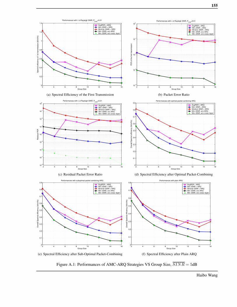
155
2 4 6 8 10 12 14 160
0.2
0.4
0.6
0.8
1
1.2
1.4
Group Size
Spe
ctra
l effi
cien
cy o
f 1st
tran
smis
sion
(bit/
s/H
z)
Performances with i.i.d Rayleigh SINR, PLoss
=0.01
AvgPER + ARQMin−SINR + ARQMin2nd−SINR + ARQMin−SINR, w/o ARQMin−SINR, w/o cross−layer
(a) Spectral Efficiency of the First Transmission
2 4 6 8 10 12 14 1610−4
10−3
10−2
10−1
100
Group Size
PE
R o
f the
firs
t tra
nsm
issi
on
Performances with i.i.d Rayleigh SINR, PLoss
=0.01
AvgPER + ARQMin−SINR + ARQMin2nd−SINR + ARQMin−SINR, w/o ARQMin−SINR, w/o cross−layer
(b) Packet Error Ratio
2 4 6 8 10 12 14 1610−8
10−7
10−6
10−5
10−4
10−3
10−2
10−1
100
Group Size
Res
idua
l PE
R
Performances with i.i.d Rayleigh SINR, PLoss
=0.01
AvgPER + ARQMin−SINR + ARQMin2nd−SINR + ARQMin−SINR, w/o ARQMin−SINR, w/o cross−layer
(c) Residual Packet Error Ratio
2 4 6 8 10 12 14 160
0.1
0.2
0.3
0.4
0.5
0.6
0.7
0.8
0.9
Group Size
Ove
rall
Spe
ctra
l effi
cien
cy (b
it/s/
Hz)
Performances with optimal packet combining ARQ
AvgPER + ARQMin−SINR + ARQMin2nd−SINR + ARQMin−SINR, w/o ARQMin−SINR, w/o cross−layer
(d) Spectral Efficiency after Optimal Packet-Combining
2 4 6 8 10 12 14 160
0.1
0.2
0.3
0.4
0.5
0.6
0.7
0.8
0.9
Group Size
Ove
rall
Spe
ctra
l effi
cien
cy (b
it/s/
Hz)
Performances with suboptimal packet combining ARQ
AvgPER + ARQMin−SINR + ARQMin2nd−SINR + ARQMin−SINR, w/o ARQMin−SINR, w/o cross−layer
(e) Spectral Efficiency after Sub-Optimal Packet-Combining
2 4 6 8 10 12 14 160
0.1
0.2
0.3
0.4
0.5
0.6
0.7
0.8
Group Size
Ove
rall
Spe
ctra
l effi
cien
cy (b
it/s/
Hz)
Performances with plain ARQ
AvgPER + ARQMin−SINR + ARQMin2nd−SINR + ARQMin−SINR, w/o ARQMin−SINR, w/o cross−layer
(f) Spectral Efficiency after Plain ARQ
Figure A.1: Performances of AMC-ARQ Strategies VS Group Size, SINR = 5dB
Haibo Wang

156 Chapter A. Additional Results of the Cross-Layer Strategies
2 4 6 8 10 12 14 161.4
1.6
1.8
2
2.2
2.4
2.6
2.8
3
3.2
Group Size
Spe
ctra
l effi
cien
cy o
f 1st
tran
smis
sion
(bit/
s/H
z)Performances with i.i.d Rayleigh SINR, P
Loss=0.01
AvgPER + ARQMin−SINR + ARQMin2nd−SINR + ARQMin−SINR, w/o ARQMin−SINR, w/o cross−layer
(a) Spectral Efficiency of the First Transmission
2 4 6 8 10 12 14 1610−4
10−3
10−2
10−1
100
Group Size
PE
R o
f the
firs
t tra
nsm
issi
on
Performances with i.i.d Rayleigh SINR, PLoss
=0.01
AvgPER + ARQMin−SINR + ARQMin2nd−SINR + ARQMin−SINR, w/o ARQMin−SINR, w/o cross−layer
(b) Packet Error Ratio
2 4 6 8 10 12 14 1610−8
10−7
10−6
10−5
10−4
10−3
10−2
10−1
100
Group Size
Res
idua
l PE
R
Performances with i.i.d Rayleigh SINR, PLoss
=0.01
AvgPER + ARQMin−SINR + ARQMin2nd−SINR + ARQMin−SINR, w/o ARQMin−SINR, w/o cross−layer
(c) Residual Packet Error Ratio
2 4 6 8 10 12 14 161.4
1.6
1.8
2
2.2
2.4
2.6
2.8
Group Size
Ove
rall
Spe
ctra
l effi
cien
cy (b
it/s/
Hz)
Performances with optimal packet combining ARQ
AvgPER + ARQMin−SINR + ARQMin2nd−SINR + ARQMin−SINR, w/o ARQMin−SINR, w/o cross−layer
(d) Spectral Efficiency after Optimal Packet-Combining
2 4 6 8 10 12 14 161.4
1.6
1.8
2
2.2
2.4
2.6
2.8
Group Size
Ove
rall
Spe
ctra
l effi
cien
cy (b
it/s/
Hz)
Performances with suboptimal packet combining ARQ
AvgPER + ARQMin−SINR + ARQMin2nd−SINR + ARQMin−SINR, w/o ARQMin−SINR, w/o cross−layer
(e) Spectral Efficiency after Sub-Optimal Packet-Combining
2 4 6 8 10 12 14 161.2
1.4
1.6
1.8
2
2.2
2.4
2.6
2.8
Group Size
Ove
rall
Spe
ctra
l effi
cien
cy (b
it/s/
Hz)
Performances with plain ARQ
AvgPER + ARQMin−SINR + ARQMin2nd−SINR + ARQMin−SINR, w/o ARQMin−SINR, w/o cross−layer
(f) Spectral Efficiency after Plain ARQ
Figure A.2: Performances of AMC-ARQ Strategies VS Group Size, SINR = 15dB
Aalborg Universitet

Appendix B
List of Abbreviations
3GPP Third Generation Partnership Project
ACK Acknowledgement
ADC Analog-to-Digital Converter
ADSL Asymmetric Digital Subscriber Line
AM Adaptive Modulation
AMC Adaptive Modulation and Coding
ARQ Automatic Repeat reQuest
AWGN Additive White Gaussian Noise (AWGN)
BER Bit Error Ratio
BPSK Binary Phase Shift Keying
BS Base Station
CATV Cable Television
CDF Cumulative Distribution Function157

158 Chapter B. List of Abbreviations
CDMA Code Division Multiple Access
CP Combined Packet
CSI Channel State Information
DAB Digital Audio Broadcasting
DAC Digital to Analogue Converter
DVB-T Digital Video Broadcasting - Terrestrial
ED Error Detection
FDMA Frequency Division Multiple Access
FEC Forward Error Correction
FFT Fast Fourier Transform
GBN Go-Back-N
GSM Global System for Mobile Communications
HARQ Hybrid Automatic Repeat reQuest
HSDPA High-Speed Downlink Packet Access
HSUPA High-Speed Uplink Packet Access
IETF International Engineering Task Force
IFFT Inverse Fast Fourier Transform
i.i.d Independent Identical Distributions
ISI Inter-Symbol interferenceAalborg Universitet

159
LA Link Adaptation
LOS Line-Of-Sight
LTE Long Term Evolution
MBMS Multimedia Broadcast and Multicast Service
MCM Multiple Carrier Modulation
MIMO Multiple Input Multiple Output
MT Mobile Terminal
OFDM Orthogonal Frequency Division Multiplexing
OFDMA Orthogonal Frequency Division Multiple Access
PER Packet Error Ratio
PDF Probability Density Function
PDU Packet Data Unit
PTM Point to Multi-point
PTP Point to Point
QAM Quadrature Amplitude Modulation
QoS Quality of Service
QPSK Quadrature Phase-Shift Keying
RF Radio Frequency
RFC Request for CommentsHaibo Wang

160 Chapter B. List of Abbreviations
RRM Radio Resource Management
RUNE Rudimentary Network Emulator
SAW Stop-And-Wait
SCM Single Carrier Modulation
SINR Signal-to-Interference-and-Noise-Ratio
SNR Signal-to-Noise-Ratio
SR Selective Retransmission
TS Time-Slots
TTI Transmission Time Interval
UE User Equipment
UMTS Universal Mobile Telecommunications Systems
UTRAN Universal Terrestrial Radio Access Network
WCDMA Wide-band Code Division Multiple Access
WiMAX Worldwide Inter-operability for Microwave Access
WLAN Wireless Local Area Networks
Aalborg Universitet

Appendix C
List of Math Notations and Symbols
Chapter 2
L : the path-loss in decibels (dB);
n : the path-loss exponent, no unit;
d : the distance between the transmitter and the receiver in meters;
C : a constant which depends on the carrier frequency, environment type (e.g.,
rural, urban, suburban, indoor), and other system loss factors, in decibels;
Td : delay spread, is defined as the time difference between the first and the last
received impulses, measured in s, ms or ns;
t : time;
τi(t), τj(t) : the arrival time of two impulses from the same transmitted signal
due to multipath;
Bc : coherence bandwidth in Hz;
Bs : bandwidth of a baseband symbol in Hz;161

162 Chapter C. List of Math Notations and Symbols
f : frequency in Hz;
S(f) : power function along frequency domain, usually in watt;
G(f) : channel gain function along frequency domain in linear unit.
Chapter 3
i : the index of multicast receivers;
j : the index of OFDM subcarriers within a multicast subchannel;
SNR(i, j) : signal-to-noise-ratio of multicast receiver i over subcarrier j;
M : the modulation mode, e.g., BPSK, 4QAM, 16QAM, 64QAM, 256QAM, or
turn-off;
KM : the number of bits per symbol on a subcarrier corresponding to a modulation
mode;
vd : the sampled complex delay profile, no unit;
Drms : the rms delay in sample unit;
Dmax : the maximum delay spread in sample unit;
wd : a complex Normal random process;
V : the normalization factor, no unit;
N : the number of mobile receivers in the investigated multicast group;
S : the user satisfaction rate, not unit;
T : the Normalized Average user Goodput per session, no unit;Aalborg Universitet

163
Goodputi : the correctly received bits by receiver i during one service session;
R(T, S) : Reward function made up of S and T , no unit;
BERi : the average BER of receiver i during the whole multicast service session;
θ : the average BER constraint, no unit, θ = 10−3;
W1, W2 : the relative weights of T and S used in Reward function definition in
Sec. 3.4;
BER(M, SNRi,j) : the instantaneous BER of receiver i on subcarrier j;
S ′(M, j) : the instantaneous satisfaction rate of mode M on subcarrier j;
T ′(M, j) : the instantaneous goodput of mode M on subcarrier j;
R′(M, j) : the local Reward of mode M on subcarrier j;
w1′, w2′ : the local/instantaneous relative weights of T ′(M, j) and S ′(M, j) used
in the instantaneous Reward function definition in Sec. 3.4;
Mopt(j) : the optimal modulation mode on subcarrier j;
ΓM : the SNR thresholds of each modulation mode;
BERc : the cumulated BER at receiver i since the multicast transmission start
until the current time;
θ1 : the arbitrary low boundary of the optimal BER interval in Sec. 3.5;
θt(i) : the instantaneous BER Threshold for the next transmission for UEi in Sec.
3.5;
θmax : the arbitrary upper boundary of θt(i) in Sec. 3.5;Haibo Wang

164 Chapter C. List of Math Notations and Symbols
δ : the multiplicative factor to increase θt(i) in Sec. 3.5.
Chapter 4
N : the number of receivers in a multicast group;
C : Shannon capacity of a channel, in bit/s;
B : channel bandwidth, in Hz;
R : achievable data rate of practical system, bit/s;
Υ : the gap between Shannon capacity and the achievable capacity/capacity of
real systems, no unit;
x : the transmitted multicast signal amplitude in volt;
gi : the channel gain of receiver i;
σi : the noise amplitude at receiver i in volt;
yi : the received signal amplitude at receiver i, in volt;
γi : the instantaneous Normalized SNR measured under average transmitted power
level, in linear unit in all math expressions, but presented in decibels in all fig-
ures;
SNRi : the received SNR of receiver i after power adaptation, in linear unit in
math expressions, but in decibels in all figures;
~γ : a random fading state vector, made up of all the instantaneous γi of the multi-
cast group receivers;Aalborg Universitet

165
p∗(~γ) : the probability density function of ~γ;
k : transmitted data rate as a function of ~γ in this chapter, bits per symbol;
Ts : duration of a baseband symbol;
S : power in watt, a function of ~γ in this chapter;
θ : BER constraint, theta = 10−3 in this chapter;
(R/B)T : transmitted spectral efficiency in bits/s/Hz;
(RB )i : received spectral efficiency by receiver i, in bits/s/Hz;
(RB ) : average spectral efficiency among all multicast receivers;
E. : the mathematical expectation of a random variable;
S : the average power constraint, in watt;
Ω : a region of ~γ in the non-negative N-dimensional space;
(R+0 )N : a space of N-dimensional space with non-negative real values on each
dimension;
J (.) : the Lagrange function;
λ0 : the Lagrange multiplier for the power constraint;
σ : an arbitrary function;
ε : a sufficient small number;
c : a constant, no unit;
Sopt : the optimal power adaptation function;Haibo Wang

166 Chapter C. List of Math Notations and Symbols
γ0 : a threshold of the normalized SNR to turn-on the transmission on the multi-
cast channel;
∆, α : two arbitrary values derived from the multi-dimensional integrations.
Sc : the constant transmission power level average power constraint, in watt;
SL : a linear power function, in watt;
β, ϕ : parameters of the linear power function, no unit;
(
R
B
)
Shannon: Shannon capacity of a multicast channel under the worst-link-dominant
limit.
Chapter 5
N : the total number of receivers in a multicast group;
m : index of AMC mode;
P : average packet loss ratio;
K : number of original data packets to be coded;
L : (in page 81) number of output packets after the packet encoder;
Tmaxr : maximum allowed number of retransmissions;
Ploss : residual packet loss/error ratio after retransmissions;
P0 : the expectation of the instantaneous packet error ratio of a transmission;
PERm(.) : packet error ratio estimation function of transmission mode m (a
AMC mode);Aalborg Universitet

167
am, gm : parameters depend on AMC mode, no unit;
Γm : AMC threshold of mode m corresponding to Ploss;
Γ′m : AMC threshold of mode m corresponding to P0;
Se : spectral efficiency in bits/s/Hz;
Rm : bits per symbol of AMC mode m;
T : the overall expected number of transmissions to correctly deliver an original
packet;
η : packet combining efficiency, 1 divided by the number of data packets included
in 1 combined packet;
L : (since page 86) the number of receivers which lost a same packet;
j : packet index;
k : index of receivers;
D. : an original data packet, to be distinguished with the retransmitted combined
packet;
PERm : instantaneous average PER of AMC mode m among the group;
mopt : the optimal instantaneous AMC mode;
i : index of the receiver which lost a packet.
Haibo Wang