1

Investigating the effect of learning in set-up cost for imperfect production systems by utilizing two-

way inspection plan for rework under screening constraints

Aakanksha Kishore, Prerna Gautam, Aditi Khanna*, Chandra K. Jaggi Department of Operational Research,

Faculty of Mathematical Sciences, University of Delhi,

Delhi-110007, India

Abstract- In the modern industrial environment, there is a continuous need for the advancement and

improvement of the organization’s operations. Learning is an inherent property which is time-dependent

and comes with experience. In view of this, the present framework considers the process of learning for

an imperfect production system which aids in reducing the setup cost with the level of maturity gained,

hence, providing positive results for the organization. Because of machine disturbances/ malfunctions,

defectives are manufactured with a known probability density function. To satisfy the demand with good

products only, the manufacturer invests in a two-way inspection process with multiple screening

constraints. The first inspection misclassifies some of the items and delivers inaccuracies, viz., Type-I and

Type–II. The loss due to inspection at the first stage is managed efficiently through a second inspection

which is presumed to be free from errors. The study mutually optimizes the production and backordering

quantities in order to maximize the expected total profit per unit time. Numerical analysis and detailed

sensitivity analysis is carried out to validate the hypothesis and further cater to some valuable

implications.

Keywords: Inventory; Imperfect-production; Two-way inspection; Sales-returns; Learning; Screening-

constraints

*Corresponding Author. Mob: +91 9911007707; Tel. Fax: +91 11 27666672

E-mail: kishore.aakanksha@gmail.com, prerna3080@gmail.com,

dr.aditikhanna.or@gmail.com*, ckjaggi@gmail.com

2

1. Introduction and literature overview

The following section showcases the inspiration behind the developed framework and presents the

overview of literature in the field of inventory management relevant to the present study. In this way, the

contribution of the present framework is established among the existing literature.

1.1. Motivation

Production systems prone to malfunctions have gained a lot of attention from researchers at some time or

the other. These have been explored under imperfect environments where either the manufacturing

process could be imperfect or the screening process or possibly both. In all cases, the result is a higher

percentage of defective items that are generally preferred for rework so as to make these as good as new,

while others are conventionally salvaged at a lower price without any further check due to the screening

errors. So, many papers have adopted only a single inspection technique to separate out the defectives

from the produced lot before sending them to the market even in imperfect inspection environment. In

view of this, a lesser explored area of two-way inspection plans is emphasized in this paper in which the

first one is prone to errors while the second is assumed to be error-free. The first inspection leads to Type-

I and Type-II errors. Due to Type-I errors the revenue is directly affected as the non-defectives are

classified as defectives. However, as a result of Type-II errors, the defectives are sold to the customers

and it results into sales returns, thereby hampering the goodwill of the firm. Henceforth, through a second

inspection plan, the outcome of Type-I error can be completely saved from scraping off by mistake,

resulting in an increase in revenue. Also, second inspection plan categorizes items in three divisions

namely, perfect, reparable, and scrap items, instead of two usual categories viz. reparable and non-

reparable. Such a division aids in raising the count of perfect items in the inventory which are sold at the

markup price, which ultimately leads to higher profits. Further, learning process is an inherent property of

any organization and the maturity gained with time must be incorporated to fetch economic benefits. In

lieu of this, learning in the case of production cost components is considered, which is indeed helpful in

gaining profits for subsequent inventory cycles. Thus, the present paper considers a production run-time

dependent set-up cost to moderate the overall expenses of the system. In this way, the current study

fulfills the research gap by constructing an inventory model that deals with imperfect production systems,

two-way inspection plans, inspection errors, rework, backorders and learning in setup cost.

1.2. Literature Review

Imperfect Quality and Screening Errors: While considering manufacturing systems it is important to

take into account the malfunctions as they lead to defective items which directly result in an economic

loss for the organization. Moreover, it is necessary to manage the defectives so as to extract the monetary

value of the products as much as possible. The defectives can be categorized into reworkable and non-

reworkable items. The non-reworkable items can either be vended to a subordinate market at a cheap rate

or can be disposed of at some cost. The pioneer work in the field of imperfect production systems was

done by Porteus [1], Rosenblatt and Lee [2], Lee and Rosenblatt [3], Kim and Hong [4], Ben-Daya and

Hariga [5], Salameh and Jaber [6], Cardenas Barron [7], Huang [8], Chung and Hou [9], Yeh et al [10],

Ben-Daya and Rahim [11], Huang [12], Hsieh and Lee [13], Chen and Lo [14], and Wee et al [15]. While

dealing with imperfect quality items it is mandatory to adopt screening process, further the screening

process can have some human errors thus, it is reasonable to incorporate screening errors in the inventory

model so as to make it close to real time manufacturing process. Raouf et al. [16] were the pioneer

contributors in the field of inspection; they incorporated the effect of human errors in their model. Later,

Duffuaa and Khan [17] and Duffuaa and Khan [18] extended the work for the case of misclassifying the

3

good items into bad ones and vice-versa. Further, Zhou et al [19], Al-Salamah [20], Khan et al [21],

Khanna et al [22], Pal and Mahapatra [23], Sett et al [24] recently explored the area of inspection errors

with other realistic scenarios of inventory management.

Imperfect Quality and Rework: To compensate the failure of raising profit margins majorly due to

misclassifications which result in sale and salvage of defectives, it is many a times found useful to

implement rework process apart from planning of backorders. Also, shortages are bound to occur

whenever there is a difficulty of supply and demand especially in imperfect quality environment. Long

back, Hayek and Salameh [25] looked into the significance of rework when there are defective items in

the inventory system of finite production model with shortages. In several production systems, imperfect

items are preferred for rework, which significantly reduces the overall costs of production and inventory.

Some significant contributions made in this field are those of Chiu [26], Chiu et al [27], Chiu et al [28],

Chiu et al [29], Sana [30], Sarkar et al [31], Sarkar et al [32], Dey and Giri [33]. Later, Chiu [34], Lin

[35], Yoo et al [36] explored the area of inventory modeling with imperfect items, screening process and

rework. Recently, Hsu and Hsu [37] and Wee et al [38] developed an optimal replenishment model with

defective items, screening errors, shortages and sales returns. Cárdenas-Barrón et al. [39] put forth a

pioneer work through a brief introduction to the inventory papers. Taleizadeh et al. [40] proposed an

optimal order quantity model with partial backorders and reparation of imperfect products, Wang et al.

[41] also proposed the optimal order quantity model with the consideration of screening constraints. Jaggi

et al [42], Moussawi-Haidar et al [43], Liao [44], Pal et al [45], Shah et al [46], Sekar and Uthayakumar

[47], Benkherouf et al [48], Chen [49], Shafiee-Gol [50], Jawla and Singh [51], Cárdenas-Barrón et al.

[52], Nobil et al. [53], Chung et al. [54], Nobil et al. [55] have recently explored the area of inventory

management by incorporating various rework scenarios.

Learning in Set-Up Cost: The process of learning is a time dependent process that comes into picture

when the maturity phase of the organization and its workers occurs. In particular, learning in setup cost is

a dynamic process through which setup costs can be reduced with the onset of learning in subsequent

cycles. The earlier adoption of this process was carried out by Adler and Nanda [56], Sule [57], and also

Urban [58]. The effect of learning and forgetting was incorporated in many articles thereafter. A wide

review on the topic of learning can be studied in Jaber and Bonney [59] paper. Later, many other

researchers, namely, Jaber and Bonney [60], Jaber [61], and also Darwish [62] followed the process of

learning in their inventory modeling. Soon after, Khan et al [63] presented an inventory model with

defective items and learning in inspection. Later, Konstantaras [64] extended the model of Khan et al [63]

by incorporating shortages. Recently, Mukhopadhyay and Goswami [65] proposed an imperfect

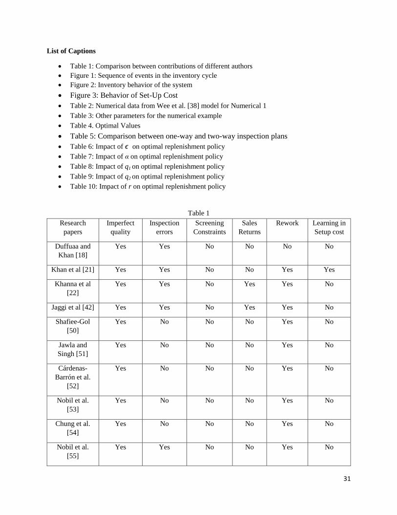
production inventory model for three kinds of defectives with rework and learning in setup. Table 1 gives

a quick review of the literature and research gaps filled.

<Insert Table 1>

Our Contribution: Inventory management revolves around products and customers. The process of

managing products is categorized into numerous parts implementing all the required activities viz.

manufacturing, screening, rework, and sales refunds-when the end consumer is not satisfied. Therefore, it

makes absolute sense to incorporate product management that includes the control of perfect and

imperfect both kinds of products for realistic inventory modeling. In order to manage the whole lot

efficiently, firstly an “error-prone” screening process is employed on the complete batch that discards

some perfect products by mistake (an outcome of Type-I error) and also sells some defectives as perfect

items erroneously (an outcome of Type-II error). In order to reduce the loss due to compromised

screening at first hand, another screening process takes place simultaneously on the smaller lot of

accumulated defectives (consisting of both actual and wrongly classified defectives) under rigorous

4

surveillance at a relatively higher cost than the first inspection process. As this re-inspection is considered

to have been conducted with better quality, it comes out to be error-free and successfully nullifies the loss

occurred due to Type-I error by extracting out the perfect items (that are wrongly classified as defectives)

completely. Finally, this second inspection successfully categorizes the accumulated defectives into three

parts viz. perfect, reparable, and non-reparable. Thus, it contributes in raising the count of perfect items

and hence the revenue against an additional investment in a second inspection process. Post these two

simultaneous screening processes, the rework process begins on the reparable lot which further adds to

the revenue, at a marginal cost of rework. So, contrary to the previous research practices that assume

single and perfect inspection to handle the defectives, the present paper investigates the imperfect

production systems under the conditions of two-way inspection processes with screening errors in the first

stage only along with sales returns. A rework process is then employed for accumulated defectives under

various screening constraints for achieving higher standards of quality and thereby revenue. Additionally,

learning in setup cost is considered in the model to gain some maturity with time to elevate the profit

values. Two mathematical models are proposed for imperfect production system with and without the

effects of learning respectively. The numerical analysis and sensitivity analysis are carried out to

showcase key features. Further, the importance of two-way inspection plan is signified through a

comparative study. The model is applicable to a variety of manufacturing industries that target high

standards of quality, customer satisfaction, encourage teamwork, and prefer to invest in learning.

2. Model development

The present segment gives the notations, assumptions and constraints under which the model is

developed.

2.1. Notations

Parameters

Λ Demand rate in units per unit time

Φ Production rate

φ1 Rework rate

x Inspection rate in units per unit time, λ>D

α Proportion of imperfect items (a random variable with known p.d.f.)

q1 Proportion of Type-I imperfection error (a random variable with known p.d.f.)

q2 Proportion of Type-II imperfection error (a random variable with known p.d.f.)

p1 Proportion of non-reparable/ scrap items (a random variable with known p.d.f.)

p2 Proportion of reparable items (a random variable with known p.d.f.)

p3 Proportion of perfect items, secluded from second inspection process (a random

variable with known p.d.f.)

r Proportion of rework items (a random variable with known p.d.f.)

T Cycle length

E(.) Expected value operator

E(θ) Expected value of θ

K0 Production set-up cost for each cycle

cP Purchase cost per item ($/ item)

i1 Inspection cost per item during production ($/ item)

i2 Inspection cost per item after production ($/ item)

s Selling price ($/ item)

5

u Disposal cost of defectives(< s) ($/ item)

v Unit discounted price of each defective item (< s) ($/ item)

cB Shortage cost per unit per unit time

cr Cost of obligating Type-I error ($/ item)

ca Cost of obligating Type-II error ($/ item)

h Holding cost per unit time

h1 Holding cost of reworked items per unit time

Decision variables

y Production lot size

B Backorder level

Functions

f(α) p.d.f. of defective items

f(q1) p.d.f. of Type-I error

f(q2) p.d.f. of Type-II error

f(r) p.d.f. of rework items

f(p1) p.d.f. of scarp items

f(p2) p.d.f. of non-repairable items

f(p3) p.d.f. of repairable items

T.C. Total cost

E.T.C.U. Expected total cost per unit time

T.R. Total revenue

E.T.R.U. Expected total revenue per unit time

Zj(y,B) Total profit per unit time for j = 1,2

E[Zj(y,B)] Expected total profit per unit time for j = 1,2ime

Optimal values

T* Optimal cycle length

y* Optimal order quantity per cycle

B* Optimal Backorder level

E[Z*(y,B)] Optimal expected total profit per unit time

2.2. Assumptions

The mathematical model has been proposed under the following assumptions.

1) Demand rate is constant, uniform and deterministic. Also demand is satisfied by perfect items

only.

2) Production rate is finite and constant.

3) Production process produces only single product type and delivers some imperfect items as well.

4) First screening process leads to Type-I and Type-II misclassification errors.

5) Second stage inspection is error free and produces three types of items, namely, perfect,

repairable, and non-repairable items.

6) Rework process is considered after the end of second inspection procedure.

7) The screening cost during production is higher than the screening cost after production.

8) The holding cost of defectives that are reworked is more than that of non-defective items.

9) The manufacturer is learning from past experience and is able to reduce the set-up time and cost

eventually.

10) The non-learning model can be the trivial case of the present study, i.e., 0

6

11) Shortages are allowed and fully backlogged.

12) Time period is infinite and lead time is insignificant.

2.3. Model Constraints

1) Production rate is greater than screening rate (ϕ >x).

2) Rate of screening is greater than the rate of demand (x>λ).

3) Rate of rework is greater than the demand rate (ϕ >λ).

4) Since some perfect items will always be there in the inventory, so 11 E p 0 .

5) In order to eliminate the backorders and maintain the positive inventory, we have

11 E p x 0 .

6) In order to avoid the shortages during the screening process, the number of inspected perfect

items should be at least equal to the demand during that period i.e. 1

yy 1 E p

x

.

7) Production rate of perfect items satisfies the inequality: 11 E p x .

2.4. Screening Constraints

1) When the production rate is greater than the screening time, the screening process will continue

even after the production process i.e. 4t 0 .

2) For smooth functioning of inventory, screening should finish before the completion of inventory

i.e. 4 5 6t t t .

3) The total expected cost of production along with screening should be less than the total sales

revenue earned by selling both perfect and imperfect items i.e.

p 1 2 2c d d s 1 s q s r v 1 r

3. Mathematical modeling

The present segment describes the problem definition so as to give the clear picture of the problem under

consideration and formulates the mathematical model that fits the above discussed assumptions and

constraints.

3.1. Problem Definition

Manufacturing systems are loaded with a number of sub units and due to reasons like interrupted supply

of power, age based issues, tools malfunction, overheating of the machine etc. the system can end up

producing defectives. The defective items should be removed from the lot by a vigilant screening process.

However, the screening is not always error-free because of numerous reasons like lack of good work

instructions, some human errors, weak control over the entire screening process etc. which ultimately

leads to misclassification errors of two types namely Type-I and Type-II. The first type of error results in

direct loss of revenue for the manufacturer and due to the second type of error, the defective items are

delivered to the customers who bring sales returns. To reduce the harm related to the goodwill of the

manufacturer in the market, sales returns are also legitimate for full price refunds. For the effective

management of the whole inventory system, the management of all the items that are either actually

defective or wrongly classified as defective or that are returned from the customers is vital. Due to the

outcome of Type-I error, there arises a need for another inspection process that is capable of not only

saving the perfect items from getting scrapped at a reduced price or getting them reworked for no use, but

also extracting them successfully at a marginal cost of second inspection process only. In view of this, the

7

second inspection process is considered to be error-free and thus it caters the manufacturer with three

types of products viz. non-reparable (p1 = α (1-r)), reparable (p2 = αr), and the perfect ones (p3 = (1-

α)q1), which were particularly victimized by the Type-I error earlier. Further, a rework process is

employed in order to transform the items of reparable category into perfect ones at some rework cost.

Also, the process of learning is an ongoing time-dependent process and learning in the setup of the

production process is of great importance for the manufacturer. With time, the organization is able to

learn numerous things which should be incorporated in the subsequent production cycles in order to

increase the efficiency of the firm. In light of this, the present framework develops two cases for an

inventory model with and without the effects of learning in setup cost in the presence of defectives, two

stage inspection process, screening errors in the first inspection procedure, perfect rework process,

disposal of non-reparable stock, and also incorporates fully backlogged shortages.

Thus, the proposed model has been explored under many realistic model constraints as well as screening

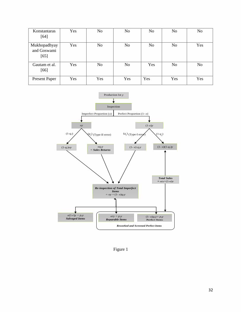
constraints so as to attain more practical results. The sequential flow of above described events is given in

Figure 1.

<Insert Figure 1>

The problem of the manufacturer is formulated by jointly optimizing the optimal production batch size

and backorder size. Profit is obtained by subtracting all the cost components viz. cost of production,

inspection, misclassification, rework, shortage, disposal and holding from the revenue which is obtained

by the sales of good items, imperfect items, and reworked items. Further, the fractions of Type-I and

Type-II errors are considered independent of defect proportion.

3.2. Mathematical Formulation

The present fragment formulates a mathematical model which fits the problem description and

assumptions of the model. The graphical representation of the inventory is given in Figure 2.

<Insert Figure 2>

Total outcome of perfect items sorted after the combined effect of inspection and rework processes are

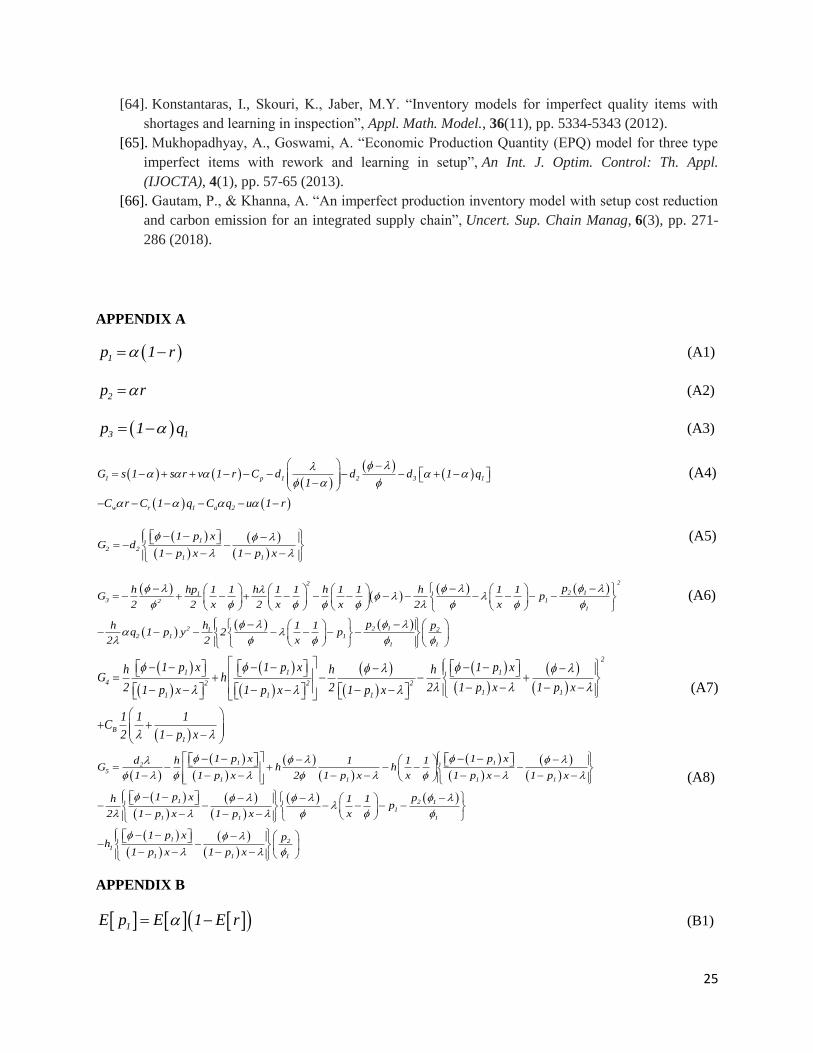
11 p y

where 1p is expanded in APPENDIX A

Since demand is satisfied from perfect items only so the length of total cycle is defined as the total

number of perfect items sold as per the demand rate i.e.

1

yT 1 p

(1)

Shortages start building up from the beginning of the inventory cycle i.e. from time 0 to A1, so the total

backorder building time is calculated as1

Bt

(2)

After time point A1, shortages begin to reduce and get completely eliminated by A2, so the complete

shortage elimination time is determined by

2

1

Bt

1 p x

(3)

8

Also, the whole inventory of defectives built during the shortage removal time (A1,A2) is estimated as:

1

1 1 2

1

1 p x Bz 1 p x t

1 p x

(4)

The overall inventory during time period (A2,A3) is constructed by the accumulation defectives as well as

the unsold perfect items. The uptime of this inventory is calculated as:

15 1

3 5

1

1 p x Bz z 1t z

1 p x

(5)

Also, the entire production runs for a period of A1up to A3, so its duration can be obtained by adding

lengths 2t , 3t i.e. 2 3

yt t

(6)

By substituting the value of equation (3) in above equation,

3

1

y Bt

1 p x

(7)

On equating equations (5) and (7), the value of z5 is obtained as:

1

5

1 1

1 p x B y Bz

1 p x 1 p x

(8)

As the total screening time is presumed to exceed the production time, therefore, it varies from time point

A1 to A4 and is given as 2 3 4

yt t t

x

(9)

By substituting the value of equation (6) in above equation, 4

y yt

x (10)

Also, the total inventory depleted during the post production screening time is determined as:

5 4 4z z t (11)

By using equations (8), (10), and (11), the value of z4 is obtained as:

1

4

1 1

1 p x B y B y yz

1 p x 1 p x x

(12)

The defectives which are scrapped add up top1y and these are disposed right after the end of screening

process i.e. at A4, so the effective inventory gets reduced instantaneously and is given by:

1

3 4 1 1

1 1

1 p x B y B y yz z p y p y

1 p x 1 p x x

(13)

Next, the rework process of a fraction from total accumulated defectives begins subsequent to the second

inspection procedure. The second inspection is done on hand-to-hand basis and so its time period is not

taken into account. So, the rework runtime which begins from A4 and continues till A5 is determined as:

9

13 2

5 1 2

1 1 1 1

1 p x Bz z 1 y B y yt p y z

1 p x 1 p x x

(14)

Also, out of the entire defective inventory αy, the count of reworkables is 2p y , so the rework processing

time can also be rewritten as 2

5

1

p yt

(15)

On equating equations (14) and (15), the value of z2 is obtained as:

1 2 1

2 1

1 1 1

1 p x B p yy B y yz p y

1 p x 1 p x x

(16)

Lastly, the remaining perfect items coming out of the rework process ( 2p y ) and also those which are

directly segregated from the second inspection process ( 3p y ) get sold till the inventory completely

depletes to zero. So, we have,

1 2 126 1

1 1 1

1 p x B p yz 1 y B y yt p y

1 p x 1 p x x

(17)

Since whole screening process is covered in two parts, one part ends with the production procedure and

thus runs for a length of (t2 + t3) while the second part begins after the production process is over and runs

for a length of (t4) i.e. till all the remaining items are screened. So, the number of units screened during

the first interval (A1, A3) is obtained in the following manner:

2 32

2 3

t t y.... t t

1 1

(18)

Ay , where,

A1

(19)

To estimate the total number of units screened during the second interval (A3, A4), we first determine the

complete count of defectives accumulated bytimepointA3and then subtract these from the maximum

inventory level present at that time i.e. 5z . The total number of defectives accumulated during (A3, A4) is

obtained by the total units screened by time point A3 minus the demand satisfied by this time i.e.

1Ay t

(20)

Hence, by using equation (20), the total number of items screened between (A3, A4) is as follows:

5 1z Ay t

(21)

1

1 1

1 p x B y B yB

1 p x 1 p x 1

(22)

10

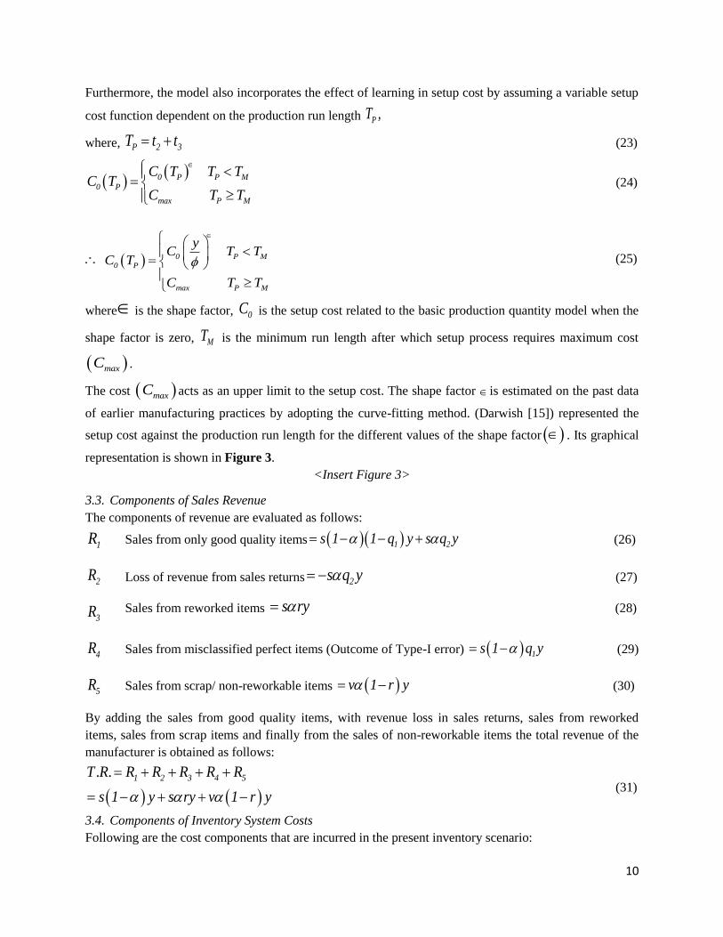
Furthermore, the model also incorporates the effect of learning in setup cost by assuming a variable setup

cost function dependent on the production run length PT ,

where, P 2 3T t t (23)

0 P P M

0 P

max P M

C T T TC T

C T T

(24)

0 P M

0 P

max P M

yC T T

C T

C T T

(25)

where is the shape factor, 0C is the setup cost related to the basic production quantity model when the

shape factor is zero, MT is the minimum run length after which setup process requires maximum cost

maxC .

The cost maxC acts as an upper limit to the setup cost. The shape factor is estimated on the past data

of earlier manufacturing practices by adopting the curve-fitting method. (Darwish [15]) represented the

setup cost against the production run length for the different values of the shape factor . Its graphical

representation is shown in Figure 3.

<Insert Figure 3>

3.3. Components of Sales Revenue

The components of revenue are evaluated as follows:

1R Sales from only good quality items 1 2s 1 1 q y s q y

(26)

2R Loss of revenue from sales returns 2s q y

(27)

3R Sales from reworked items s ry

(28)

4R

Sales from misclassified perfect items (Outcome of Type-I error)

1s 1 q y (29)

5R Sales from scrap/ non-reworkable items v 1 r y

(30)

By adding the sales from good quality items, with revenue loss in sales returns, sales from reworked

items, sales from scrap items and finally from the sales of non-reworkable items the total revenue of the

manufacturer is obtained as follows:

1 2 3 4 5T.R. R R R R R

s 1 y s ry v 1 r y

(31)

3.4. Components of Inventory System Costs

Following are the cost components that are incurred in the present inventory scenario:

11

Setup cost, obtained by introducing the effects of learning in setup costs:

0 P M

0 P

max P M

yC T T

C T

C T T

(32)

Purchase cost including the variable cost per cycle: pC y (33)

Screening cost of first inspection process during production runtime:

1

yd

1

(34)

Screening cost of first inspection process post production:

1

2

1 1

1 p x B y B yd B

1 p x 1 p x 1

(35)

Screening cost of second inspection process: 3 1d y 1 q y

(36)

Rework Cost: wC ry (37)

Cost of Type-I error which incurs because the inspector has wrongly classified some fraction of non-

defectives as defectives: r 1C 1 q y (38)

Cost of Type-II error which incurs because the inspector has misclassified a portion of defectives as

non-defectives: a 2C q y (39)

Disposal Cost of non-reworkable items: u 1 r y

(40)

Holding cost of the defective, non-defectives and sales returns in a cycle:

1 2 3 1 5 4 5 3 6 2 2 1 3 2 5

1 1 1 1 1 1h z t t z z t z z t z q yT h z z t

2 2 2 2 2 2

(41)

Shortage Cost: B 1 2

1C t t B

2 (42)

As the present model is developed under the assumption of learning in setup cost, thus, depending upon

the learning effects two cases are established for manufacturer’s total cost:

Case I: P MT T (Under the Effects of Learning)

Considering the case when P MT T the following value is obtained for the total cost of the manufacturer

by substituting the appropriate value of 0 PC T .

12

1

0 p 1 2

1 1

1 2 3 1 5 4 5 3

3 1 w r 1 a 2

6 2 2

1 p x By y y B yT .C.1 C C y d d B

1 1 p x 1 p x 1

1 1 1z t t z z t z z

2 2 2d y 1 q y C ry C 1 q y C q y u 1 r y h

1 1t z q yT

2 2

1 3 2 5 B 1 2

1 1h z z t C t t B

2 2

(43)

The manufacturer’s total profit for Case I is expressed as follows:

1

1 1

0 p 1 2

1 p x B y B

1 p x 1 p xy yT .P.1. s 1 y s ry v 1 r y C C y d d

1 yB

1

2

1 1

3 1 w r 1 a 2 2

1 11

2

1

1 1 1

1 p x B 1 p x Bh y Bd y 1 q y C ry C 1 q y C q y u 1 r y h

2 1 p x 1 p x1 p x

2 1 p x Bh y B h y y y B2

2 1 p x 2 x 1 p x 1 p x

1

y yp y

x

2

1 2 1 2

1 2 1

1 1 1

1 p x B p yh y B y y hp y q 1 p y

2 1 p x 1 p x x 2

1 2 11 21

1 1 1 1

2

B

1

1 p x B p yh p yy B y y2 p y

2 1 p x 1 p x x

1 1 1C B

2 1 p x

(44)

2 2 01 2 3 4 5

C yyG BG y G B G yBG

(45)

where, 1p , 2 3p , p 1G , 2G ,…, 5G are expanded in APPENDIX A

The manufacturer’s total profit per unit time for Case I can be expressed as follows:

2 1

4 02 21 1 3 5

1

B G C yBG q yZ y,B G yG BG

1 p y y 2

(46)

Therefore, the expected total profit per unit time can be written as:

2 1

2 4 201 1 3 5

1

BE G B E G E E q yC yE Z y,B E G yE G BE G

y y 21 E p

(47)

where, 1E p , 2E p , 3E p , 1E G , 2E G ,…, 5E G are expanded in APPENDIX B

The above formulation of the function makes clear that when 1 , the profit function is monotonically

decreasing in y , which shows that the total cost function will be minimum when y 0; which is

13

reasonably impractical. In practice, it recommends that y should be minimum i.e. it should be as much

as required which closely follows the JIT (Just-in-Time) manufacturing philosophy. So, it is

recommended that 1 . Moreover, 0 PC T is a concave function which is increasing for 0 1

however decreasing for 0 .

The values indicating 0 signify the state when the effect of learning disables the effect of forgetting

and deterioration which results in the reduction of the setup costs with time.

Case II: P MT T (Without the Effects of Learning)

When P MT T the following expression for the manufacturer’s total cost is obtained:

1

max p 1 2

1 1

1 2 3 1 5 4 5 3

3 1 w r 1 a 2

6 2 2

1 3

1 p x By y B yT .C.2 C C y d d B

1 1 p x 1 p x 1

1 1 1z t t z z t z z

2 2 2d y 1 q y C ry C 1 q y C q y u 1 r y h

1 1t z q yT

2 2

1h z

2

2 5 B 1 2

1z t C t t B

2

(48)

The manufacturer’s total profit for Case II is expressed as follows:

1

1 1

max p 1 2

1 p x B y B

1 p x 1 p xyT .P.2 s 1 y s ry v 1 r y C C y d d

1 yB

1

2

1

3 1 w r 1 a 2 2

11

12

1 1 1

1 1

1 p x Bh y Bd y 1 q y C ry C 1 q y C q y u 1 r y h

2 1 p x1 p x

2 1 p x B y B2

1 p x B 1 p x 1 p xh y B h y y

1 p x 2 1 p x 2 x

1

y yp y

x

2

1 2 1 2

1 2 1

1 1 1

1 p x B p yh y B y y hp y q 1 p y

2 1 p x 1 p x x 2

2

1 2 11 21

1 1 1 1

2

B

1

1 p x B p yh p yy B y yp y

2 1 p x 1 p x x

1 1 1C B

2 1 p x

(49)

Thus, the manufacturer’s total profit can be written as:

14

2 2

1 2 3 4 5 maxyG BG y G B G yBG C , (50)

where, 1p , 2 3p , p , 1G , 2G ,…, 5G are expanded in APPENDIX A

The manufacturer’s total profit per unit time can be written as:

2

42 22 1 3 5 max

1

B GBG q yZ y,B G yG BG C

1 p y y 2

(51)

Therefore, the expected total profit per unit time can be written as:

2

2 4 2

2 1 3 5 max

1

BE G B E G yE E qE Z y,B E G yE G BE G C

y y 21 E p

(52)

where, 1E p , 2E p , 3E p , 1E G , 2E G ,…, 5E G are expanded in APPENDIX B

4. Optimal policy

The manufacturer aims to maximize the expected total profit per unit time by jointly optimizing the

production amount and the backorder quantity. In the following section, concavity of the objective

function is proved in the form of two lemmas.

Case I: P MT T

Lemma1. The function of manufacturer’s expected total profit per unit time for Case I is concave.

Proof. In order to prove the global concavity of the expected profit function for this case, the following

two second-order sufficient conditions of optimality should be satisfied:

2 2

1 1

2 2

22 2 2

1 1 1

2 2

, ,0; 0

, , ,and 0

E Z y B E Z y B

y B

E Z y B E Z y B E Z y B

y B y B

(4.1)

By taking first order partial derivative of 1 ,E Z y B with respect to y, we obtain

22

20

1 2 3 42 2

1

1,

1 2

E E qc yB BE Z y B E G E G E G

y E p y y

(53)

Next, by taking second order partial derivative of 1 ,E Z y B with respect to y, we obtain

32 2

0

1 2 42 3 3

1

1 2, 2 2

1

c yB BE Z y B E G E G

y E p y y

(54)

Again, by taking first order partial derivative of 1 ,E Z y B with respect to B, we obtain

15

2 4

1 5

1

2,

1

E G E G BE Z y B E G

B E p y y

(55)

Again, by taking second order partial derivative of 1 ,E Z y B with respect to B, we obtain

24

12

1

2,

1

E GE Z y B

B E p y

(56)

Also,

22 4

1 2 2

1

2,

1

E G E G BE Z y B

y B E p y y

(57)

Therefore, by using equations (57), (54) and (56) we obtain:

22 22 2 2

2 0 4

1 1 12 2 4 4

1

2 1 2, , ,

1

E G c E G yE Z y B E Z y B E Z y B

y B y B E p y y

(58)

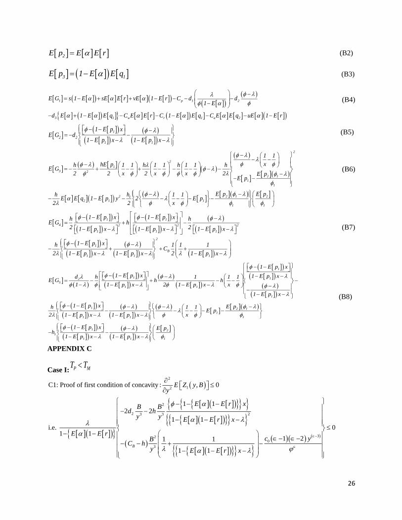
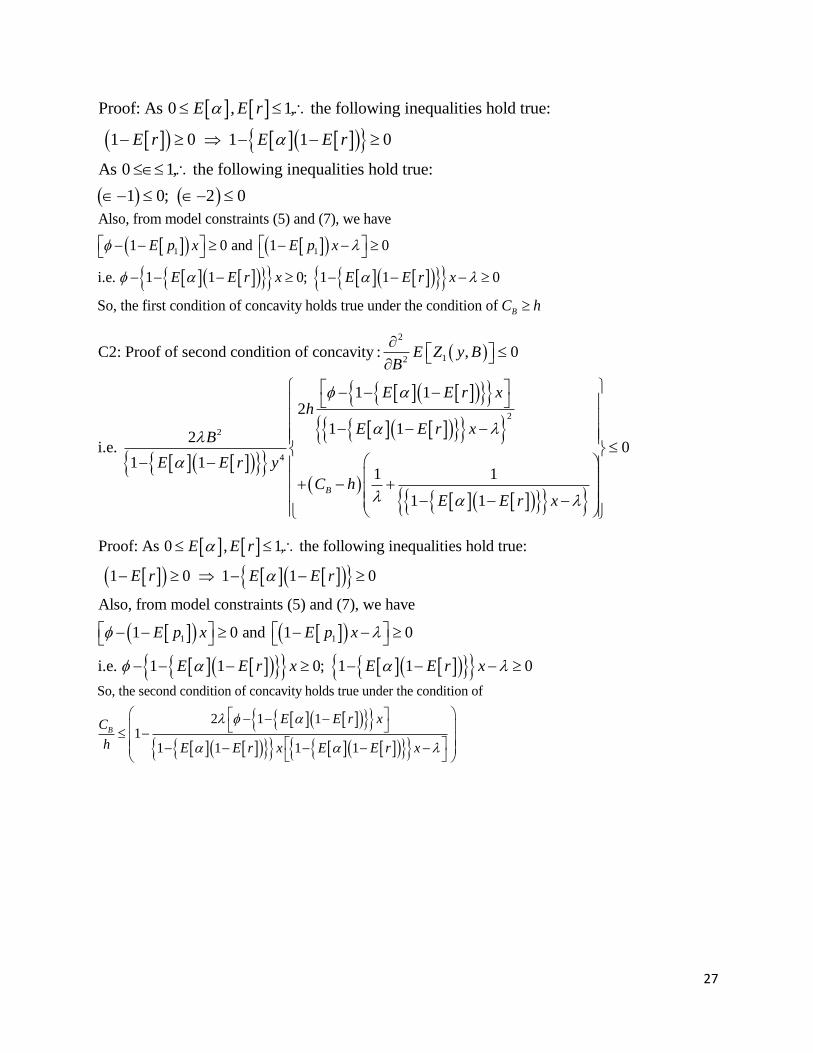
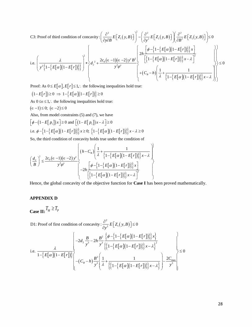
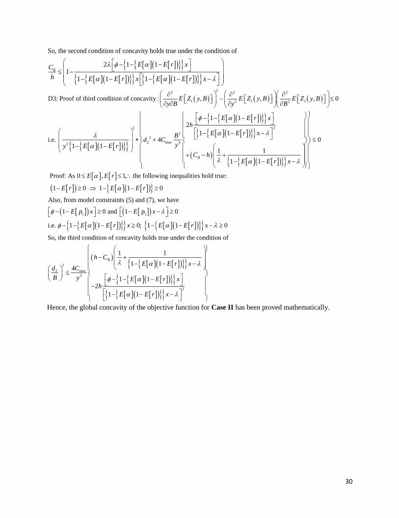
The three conditions of concavity are derived in APPENDIX C.

Lemma2. The optimal solution (y*, B*) that maximizes the manufacturer’s expected total profit per unit

time for Case I is written as:

12

0 4*

2 2

4 3 3

4 1

42

c E Gy

E E qp E G E G E G

and

2 5*

42

E G E G yB

E G

Proof. In order to find the optimal values of y and B, say y*and B*, that maximize 1 ,E Z y B , the

first-order necessary condition of optimality must be equated to zero i.e.

1 1, 0 and , 0E Z y B E Z y By B

(4.2)

On setting equation (53) equal to zero, we get:

320

2 43 3

1

1 22 2 0

1

c yB BE G E G

E p y y

(59)

On setting equation (55) equal to zero, we get:

2 4

5

1

20

1

E G E G BE G

E p y y

(60)

16

2 5*

42

E G E G yB

E G

(61)

Putting this value of B in equation (59) to attain the value for y i.e.:

12

0 4*

2 2

4 3 3

4 1

42

c E Gy

E E qp E G E G E G

(62)

Hence, y* and B* are the optimal values of y and B for Case I.

Case II: M PT T

Lemma3. The function of manufacturer’s expected total profit per unit time for Case II is concave.

Proof. In order to prove the global concavity of the expected profit function, the following two second-

order sufficient conditions of optimality for this case should also be satisfied:

2 2

2 2

2 2

22 2 2

2 2 2

2 2

, ,0; 0

, , ,and 0

E Z y B E Z y B

y B

E Z y B E Z y B E Z y B

y B y B

(4.3)

By taking first order partial derivative of 2 ,E Z y B with respect to y, we obtain

2

2max2 2 3 42 2 2

1

,1 2

E E qCB BE Z y B E G E G E G

y E p y y y

(63)

Next, by taking second order partial derivative of 2 ,E Z y B with respect to y, we obtain

2 2

max2 2 42 3 3 3

1

2, 2 2 0

1

CB BE Z y B E G E G

y E p y y y

(64)

Again, by taking first order partial derivative of 2 ,E Z y B with respect to B, we obtain

2 4

2 5

1

2,

1

E G E G BE Z y B E G

B E p y y

(65)

Again, by taking second order partial derivative of 2 ,E Z y B with respect to B, we obtain

17

24

22

1

2, 0

1

E GE Z y B

B E p y

(66)

Also, 2

2 4

2 2 2

2,

E G E G BE Z y B

y B y y

(67)

Therefore, by using equations (67), (64) and (66) we obtain

2 22 2 22 4 max

2 2 22 2 4 4

4, , ,

E G E G CE Z y B E Z y B E Z y B

y B y B y y

(68)

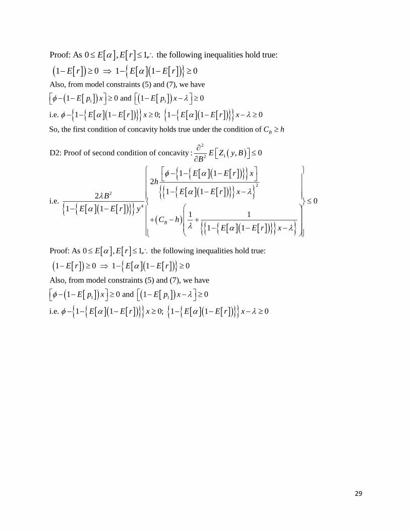
The conditions of concavity have been derived in APPENDIX D.

Lemma 4. The optimal solution (y*, B*) that maximizes the manufacturer’s expected total profit per unit

time for is written as

2

2 4 max*

3 2 1

2

2 1

BE G B E G Cy

E G E E q E p

and

2 5*

42

E G E G yB

E G

Proof. In order to find the optimal values of y and B, say y*and B*, that maximize 2 ,E Z y B , the

first-order necessary condition of optimality must be equated to zero i.e.

2 2, 0 and , 0E Z y B E Z y By B

(4.4)

On setting equation (63) equal to zero, we get:

22max

2 3 42 2 2

1

01 2

E E qCB BE G E G E G

E p y y y

(69)

2

2 4 max*

3 2 1

2

2 1

BE G B E G Cy

E G E E q E p

(70)

On setting equation (65) equal to zero, we get:

2 4

5

1

20

1

E G E G BE G

E p y y

(71)

2 5*

42

E G E G yB

E G

(72)

Putting this value of B in equation (69) to attain the value for y i.e.:

18

2

2 52 5

2 max

4 4*

3 2 1

22 4

2 1

E G E G yE G E G yE G C

E G E Gy

E G E E q E p

(73)

Hence, y* and B* are the optimal values of y and B for Case II.

5. Numerical analysis

In order to validate the developed formulation, the following section presents the numerical analysis

by illustrating two examples and solving them for each of the two cases viz. with and without the

effects of learning in set up cost. Further, this section also draws a comparison for the change in

optimal profit values between one way v/s two way inspection plans at the manufacturer’s end.

5.1 Examples

This subsection authenticates the hypothesis with the help of two examples, each solved for the above

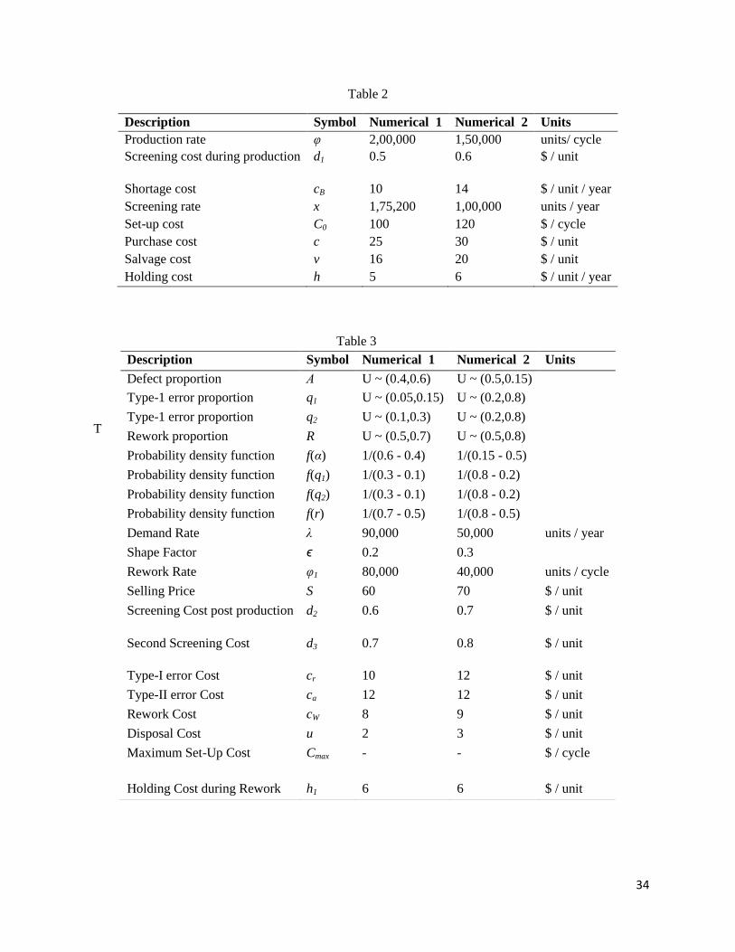
discussed cases of the learning effects. Table 2 and Table 3 demonstrate the parameter values of two

numerical examples taken similar or different from Wee et al [38] paper respectively. Table 4 depicts the

optimal values of the two examples.

<Insert Table 2>

< Insert Table 3>

< Insert Table 4>

5.2 Comparison of profit values between one way v/s two way inspection plans

This subsection derives a contrast regarding the expected total profit per unit time for the above discussed

two cases when both are solved with and without the two way inspection plans respectively.

< Insert Table 5>

Table 5 reflects that it is of great financial interest for the manufacturer to practice the second inspection

before taking the final decision of salvaging the defectives or sending the lot for rework. Another intuitive

reason to opt for second inspection plan is that it is easier to deliver quality/ error-free inspection to a

smaller batch of only accumulated defectives rather than to whole production lot. So, a small investment

in this direction pays back with higher returns. By extracting the complete fraction of wrongly classified

perfect items as defectives, the manufacturer is able to reduce his financial losses caused by committing

the Type-I error as its effect gets nullified by the re-inspection. So, even by assuming inspection errors in

the model, their impacts have been controlled proficiently.

6. Sensitivity analysis

The present section presents the robustness of the developed model by observing the change in the

objective values when the model parameters are altered.

The outcome of changes in the defect parameters α, q1, q2, r and also on the shape parameter ϵ are

observed on the optimal production quantity (y*), optimal backorder quantity (B*), optimal cycle length

19

(T*), optimal total cost per unit time (T.C.U.*), and optimal expected total profit per unit time E[Z*(y,B)]

in tabular form below.

Tables 6-10 provide the following managerial insights:

< Insert Table 6>

< Insert Table 7>

Table 6 shows that with an increase in the value of shape factor,ϵ ,the setup of production process is done

frequently which results in decreasing the backorders (B*) as there is sufficient quantity to satisfy the

demand of the retailer. The production run length (Tp*), cycle time (T*), lot size (y*) and the expected

total cost (T.C.U.*) per unit time are quite sensitive to the changes in the shape factor. The reason behind

this decrease in the loss percentage as compared to the traditional EOQ models can be explained by the

extensive crashing in the duration of the production run length and henceforth the set up cost.

As exhibited from Table 7, the value of optimal expected total profit per unit time E[Z*(y,B)] shows

declining trend along with optimal backorder level (B*), while the optimal values of production quantity

(y*), cycle length (T*), total revenue per unit time(T.R.U.*), and total cost per unit time (T.C.U.*) rise

with the increase in defect proportion (α). With an increased proportion of defects in the system, there

will be a higher sale of defectives as well as return of defectives. This not only brings considerable

monetary loss to the firm but also harms reputation. However, due to more sales of scrap items, there is an

increase of revenue but it is not able to compensate the losses incurred, so the overall profit of the system

decreases. Since demand is satisfied through perfect items only, the manufacturer needs to produce more

than the demand and hence the production quantity is observed to increase. So, it is advisable for the

operations manager to improvise his production system so as to reduce the defect proportion substantially.

< Insert Table 8>

< Insert Table 9>

From Table 8, it is observed that with increase in the proportion of Type I error (q1), the optimal

production quantity (y*), and expected value of total profit per unit time (Z*(y,B)) show declining trends

while total revenue per unit time(T.R.U.*), and total cost per unit time (T.C.U.*) reflect elevation in their

values. Due to Type-I error, there is a direct financial loss to the manufacturer as the screening process

and the inspection team is not competent enough to carry out the process without errors. Resultantly, there

is significant fall in the profit values as the non-defectives are being sold at a reduced price by mistake. In

this scenario, the manufacturer is unable to achieve maximum possible sales, so, it is beneficial for him to

reduce his production quantity so as to minimize losses related to misclassification. Revenue is indirectly

increasing by salvaging of non-defectives in a lesser restrictive inventory. However, the increase in total

cost dominates the increase in revenue, so there is a decrease in overall profit values.

It is clear from Table 9 that with increment in the proportion of Type II error(q2), there is noteworthy

decline in the optimal values of expected total profit per unit time (Z*(y,B)) and total revenue per unit

time(T.R.U.*) while the cost values show considerable increase. No significant change is observed in the

values of optimal backorder level (B*), optimal production quantity (y*), and cycle length (T*). Since

Type-II error leads to sales returns which are either entertained with full price refunds or replacement

20

with perfect products, so it impacts the revenue part majorly. Moreover, it also causes penalty and

goodwill loss to the firm which is of serious concern to the managers it also leads to increase in the cost

components. The constancy of demand and shortages is explained by the fact that the manager is able to

maintain the demand despite some sales returns. In this particular scenario, it is beneficial for the

operations manager to strengthen his screening team so as to reduce such damaging screening errors.

< Insert Table 10>

As evident from Table 10, with the increase in the proportion of reworked items (r), the optimal

production quantity (y*), cycle length (T*), total cost per unit time (T.C.U.*), and total revenue per unit

time (T.R.U.*) exhibit decreasing values while the optimal value of expected total profit per unit time

(Z*(y,B)) shows increase along with optimal backorder level (B*). It is quite logical and intuitive that

there is a cost associated with the rework process but here it also gets compensated with the rise in the

sale of perfect items. So, the overall profit of the system increases. The production quantity gets lowered

owing to the fact that due to the rework process, the count of perfect items gets increased considerably,

thereby, decreasing the need to produce more items so as to meet the demand. Consequently, the cycle

length also decreases.

7. Concluding remarks

In the current manufacturing scenario, the main challenge is to establish an efficient inventory model that

takes care of the major as well as minor concerns of the system. The problems associated with the

production system is majorly related to the production of defectives, their screening and management

thereafter. In lieu of this, the present paper develops an inventory model for finite production system

which is presumed to be imperfect and hence produces defectives at a uniform rate. To supply only good

products to the customers, the screening process plays an eminent role for the manufacturer. In contrast to

the previous studies, the present model is explored under two stages of inspection practices, with

screening errors incorporated only at the first stage. To validate the hypothesis, the numerical section

carries out the comparison of the optimal profit values in the presence of one-way and two-way inspection

techniques. Various managerial implications obtained are as follows:

The results show that the losses which were traditionally borne by the manufacturer by discarding

the perfect items by mistake (an outcome of Type-I error) in the first inspection process are

compensated with the help of small investment in the second inspection process which is error-

free.

Due to closer scrutiny in the second stage of inspection, the manufacturer is able to completely

extract the misclassified perfect items before taking the final decision of rework and hence some

undue expenses related to rework cost or unnecessary salvaging get avoided.

Even in the prevailing imperfect quality and screening environment, the manufacturer is able to

raise the revenue by selling a larger amount of perfect items at the mark-up price with respect to

the scenario of no second time inspection. So, the model successfully diminishes the relatively

harmful impact of Type-I error as compared to the effects of Type-II error.

Also, in an attempt to cut down on these escalating cost components to some extent, the process

of learning aids the manufacturer with the reduction in set-up cost of the production system in the

present model. Therefore, it makes economic sense to employ the process of learning for the

betterment of the organization as also authenticated by the decreasing loss percentage.

21

Overall, it advisable for the manufacturer to reduce the percentage of defectives through a

correct/careful production process as these elevates the defect-related costs significantly.

The model puts forth some of the very interesting and useful scenarios viz. inspection errors of Type-I

and Type-II, revenue management through two-way inspection, reduction of setup costs through time-

dependent learning, rework operations etc. Thus, the present model is preferable over the models without

the inclusion of such practical settings and it holds wide applicability in real-time manufacturing

industries.

8. Future research guidance and limitations

The model can be extended in a number of ways by adopting varying demand patterns. Also, it would be

interesting to develop an integrated vendor-buyer model in this direction. The model can also be extended

for deteriorating products, taking into account the impact of preservation technology. Consideration of

environmental factors while transportation and production, would be another worthy contribution in this

track.

The model is restricted to the scope of limited storage space for the manufacturer, also the

exactness of various cash flows in it.

References

[1]. Porteus, E.L. “Optimal lot sizing, process quality improvement and setup cost reduction”, Oper.

Res., 34(1), pp. 137-144 (1986).

[2]. Rosenblatt, M.J., Lee, H.L. “Economic production cycles with imperfect production

processes”, IIE T., 18(1), pp. 48-55 (1986).

[3]. Lee, H.L., Rosenblatt, M.J. “Simultaneous determination of production cycle and inspection

schedules in a production system”, Manage. Sci., 33(9), pp. 1125-1136 (1987).

[4]. Kim, C.H., Hong, Y. “An optimal production run length in deteriorating production

processes”, Int. J. Prod. Econ., 58(2), pp. 183-189 (1999).

[5]. Ben-Daya, M., Hariga, M. “Economic lot scheduling problem with imperfect production

processes”, J. Oper. Res. Soc., 51(7), pp. 875-881 (2000).

[6]. Salameh, M.K., Jaber, M.Y. “Economic production quantity model for items with imperfect

quality”, Int. J. Prod. Econ., 64(1), pp. 59-64 (2000).

[7]. Cárdenas-Barrón, L.E. “Observation on:“Economic production quantity model for items with

imperfect quality”[Int. J. Production Economics 64 (2000) 59–64]”, Int. J. Prod. Econ., 67(2), pp.

201 (2000).

[8]. Huang, C.K. “An integrated vendor-buyer cooperative inventory model for items with imperfect

quality”, Prod. Plan. Control, 13(4), pp. 355-361 (2002).

[9]. Chung, K.J., Hou, K.L. “An optimal production run time with imperfect production processes and

allowable shortages”, Comput. Oper. Res., 30(4), pp. 483-490 (2003).

[10]. Yeh, R.H., Ho, W.T., Tseng, S.T. “Optimal production run length for products sold with

warranty”, Eur. J. Oper. Res., 120(3), pp. 575-582 (2000).

[11]. Ben-Daya, M., Rahim, A. “Optimal lot-sizing, quality improvement and inspection errors for

multistage production systems”, Int. J. Prod. Res., 41(1), pp. 65-79 (2003).

[12]. Huang, C.K. “An optimal policy for a single-vendor single-buyer integrated production–

inventory problem with process unreliability consideration”, Int. J. Prod. Econ., 91(1), pp. 91-98

(2004).

22

[13]. Hsieh, C.C., Lee, Z.Z. “Joint determination of production run length and number of standbys in

a deteriorating production process”, Eur. J. Oper. Res., 162(2), pp. 359-371 (2005).

[14]. Chen, C.K., Lo, C.C. “Optimal production run length for products sold with warranty in an

imperfect production system with allowable shortages”, Math. Comput. Model., 44(3), pp. 319-

331 (2006).

[15]. Wee, H.M., Yu, J., Chen, M.C. “Optimal inventory model for items with imperfect quality and

shortage backordering”, Omega, 35(1), pp. 7-11 (2007).

[16]. Raouf, A., Jain, J.K., Sathe, P.T. “A cost-minimization model for multicharacteristic component

inspection”, AIIE T., 15(3), pp. 187-194 (1983).

[17]. Duffuaa, S.O., Khan, M. “An optimal repeat inspection plan with several classifications”, J.

Oper. Res. Soc., 53(9), pp. 1016-1026 (2002).

[18]. Duffuaa, S.O., Khan, M. “Impact of inspection errors on the performance measures of a general

repeat inspection plan”, Int. J. Prod. Res., 43(23), pp. 4945-4967 (2005).

[19]. Zhou, Y., Chen, C., Li, C., Zhong, Y. “A synergic economic order quantity model with trade

credit, shortages, imperfect quality and inspection errors”, Appl. Math. Model., 40(2), pp. 1012-

1028 (2016).

[20]. Al-Salamah, M. “Economic production quantity in batch manufacturing with imperfect quality,

imperfect inspection, and destructive and non-destructive acceptance sampling in a two-tier

market”, Comput. Ind. Eng., 93, pp. 275-285 (2016).

[21]. Khan, M., Hussain, M., Cárdenas-Barrón, L.E. “Learning and screening errors in an EPQ

inventory model for supply chains with stochastic lead time demands”, Int. J. Prod. Res., 55(16),

pp. 4816-4832 (2017).

[22]. Khanna, A., Kishore, A., Jaggi, C.K. “Strategic production modeling for defective items with

imperfect inspection process, rework, and sales return under two-level trade credit”, Int. J. Ind.

Eng. Comput., 8(1), pp. 85-118 (2017).

[23]. Pal, S., Mahapatra, G.S. “A manufacturing-oriented supply chain model for imperfect quality

with inspection errors, stochastic demand under rework and shortages”, Comput. Ind. Eng., 106

pp. 299-314 (2017).

[24]. Sett, B.K., Sarkar, S., Sarkar, B. “Optimal buffer inventory and inspection errors in an imperfect

production system with preventive maintenance”, T. Int. J. Adv. Manuf. Tech., 90(1-4), pp. 545-

560 (2017).

[25]. Hayek, P.A., Salameh, M.K. “Production lot sizing with the reworking of imperfect quality

items produced”, Prod. Plan. Control, 12(6), pp. 584-590 (2001).

[26]. Chiu, Y.P. “Determining the optimal lot size for the finite production model with random

defective rate, the rework process, and backlogging”, Eng. Optim., 35(4), pp. 427-437 (2003).

[27]. Chiu, S.W., Gong, D.C., Wee, H.M. “Effects of random defective rate and imperfect rework

process on economic production quantity model”, Jap. J. Ind. Appl. Math., 21(3), pp. 375-389

(2004).

[28]. Chiu, Y.S.P., Lin, H.D., Cheng, F.T. “Optimal production lot sizing with backlogging, random

defective rate, and rework derived without derivatives”, P. I. Mech. Eng. B-J. Eng., 220(9), pp.

1559-1563 (2006).

[29]. Chiu, S.W., Ting, C.K., Chiu, Y.S.P. “Optimal production lot sizing with rework, scrap rate, and

service level constraint”, Math. Comput. Model., 46(3), pp. 535-549 (2007).

23

[30]. Sana, S.S. “A production–inventory model in an imperfect production process”, Eur. J. Oper.

Res., 200(2), pp. 451-464 (2010).

[31]. Sarkar, B., Sana, S.S., Chaudhuri, K. “Optimal reliability, production lot size and safety stock in

an imperfect production system”, Int. J. Math. Oper. Res., 2(4), pp. 467-490 (2010).

[32]. Sarkar, B., Sana, S.S., Chaudhuri, K. “An economic production quantity model with stochastic

demand in an imperfect production system”, Int. J. Serv. Oper. Manag., 9(3), pp. 259-283 (2011).

[33]. Dey, O., Giri, B.C. “Optimal vendor investment for reducing defect rate in a vendor–buyer

integrated system with imperfect production process”, Int. J. Prod. Econ., 155, pp. 222-228

(2014).

[34]. Chiu, S.W. “Production lot size problem with failure in repair and backlogging derived without

derivatives”, Eur. J. Oper. Res., 188(2), pp. 610-615 (2008).

[35]. Lin, T.Y. “Optimal policy for a simple supply chain system with defective items and returned

cost under screening errors”, J. Oper. Res. Soc. Jpn., 52(3), pp. 307-320 (2009).

[36]. Yoo, S.H., Kim, D., Park, M.S. “Economic production quantity model with imperfect-quality

items, two-way imperfect inspection and sales return”, Int. J. Prod. Econ., 121(1), pp. 255-265

(2009).

[37]. Hsu, J.T., Hsu, L.F. “Two EPQ models with imperfect production processes, inspection errors,

planned backorders, and sales returns”, Comput. Ind. Eng., 64(1), pp. 389-402 (2013).

[38]. Wee, H.M., Wang, W.T., Yang, P.C. “A production quantity model for imperfect quality items

with shortage and screening constraint”, Int. J. Prod. Res., 51(6), pp. 1869-1884 (2013).

[39]. Cárdenas-Barrón, L. E., Chung, K. J., & Treviño-Garza, G. “Celebrating a century of the

economic order quantity model in honor of Ford Whitman Harris.”, Int. J. Prod. Econ., 155, pp.1-

7 (2014).

[40]. Taleizadeh, A. A., Khanbaglo, M. P. S., & Cárdenas-Barrón, L. E. “An EOQ inventory model

with partial backordering and reparation of imperfect products”, Int. J. Prod. Econ., 182, pp. 418-

434 (2016).

[41]. Wang, W.T., Wee, H.M. Cheng, Y.L., Wen, C.L., Cárdenas-Barrón, L.E. “EOQ model for

imperfect quality items with partial backorders and screening constraint”, Eur. J. Ind. Eng., 9(6),

pp. 744 – 773 (2015).

[42]. Jaggi, C.K., Khanna, A., Kishore, A. “Production inventory policies for defective items with

inspection errors, sales return, imperfect rework process and backorders”, In K. Singh, M.

Pandey, L. Solanki, S. B. Dandin, & P. S. Bhatnagar (Eds.), AIP Conf. Proc., 1715(1), pp.

020062 (2016).

[43]. Moussawi-Haidar, L., Salameh, M., Nasr, W. “Production lot sizing with quality screening and

rework”, Appl. Math. Model., 40(4), pp. 3242-3256 (2016).

[44]. Liao, G.L. “Production and Maintenance Policies for an EPQ Model with Perfect Repair,

Rework, Free-Repair Warranty, and Preventive Maintenance”, IEEE T. Syst. Man CY.-S., 46(8),

pp. 1129-1139 (2016).

[45]. Pal, S., Mahapatra, G.S., Samanta, G.P. “A Three-Layer Supply Chain EPQ Model for Price-

and Stock-Dependent Stochastic Demand with Imperfect Item under Rework”, J. Uncert. Anal.

Appl., 4(1), pp. 10 (2016).

[46]. Shah, N.H., Patel, D.G., Shah, D.B. “EPQ model for returned/reworked inventories during

imperfect production process under price-sensitive stock-dependent demand”, Oper. Res., pp. 1-

17 (2016).

24

[47]. Sekar, T., Uthayakumar, R. “A multi-production inventory model for deteriorating items

considering penalty and environmental pollution cost with failure rework”, Uncert. Sup. Chain

Manag., 5(3), pp. 229-242 (2017).

[48]. Benkherouf, L., Skouri, K., Konstantaras, I. “Optimal Batch Production with Rework Process

for Products with Time-Varying Demand over Finite Planning Horizon”, Oper. Res. Eng. Cyb.

Sec., pp. 57-68 (2017).

[49]. Chen, T.H. “Optimizing pricing, replenishment and rework decision for imperfect and

deteriorating items in a manufacturer-retailer channel”, Int. J. Prod. Econ., 183, pp. 539-550

(2017).

[50]. Shafiee-Gol, S., Nasiri, M. M., & Taleizadeh, A. A. “Pricing and production decisions in multi-

product single machine manufacturing system with discrete delivery and

rework”, Opsearch, 53(4), pp. 873-888 (2016).

[51]. Jawla, P., & Singh, S. “Multi-item economic production quantity model for imperfect items

with multiple production setups and rework under the effect of preservation technology and

learning environment” Int. J. Ind. Eng. Comput., 7(4), pp. 703-716 (2016).

[52]. Cárdenas-Barrón, L. E., Treviño-Garza, G., Taleizadeh, A. A., & Vasant, P. “Determining

replenishment lot size and shipment policy for an EPQ inventory model with delivery and

rework” Math. Prob. Eng., 2015 (2015).

[53]. Nobil, A.H., Sedigh, A.H.A., Cárdenas-Barrón, L.E. “Multi-machine economic production

quantity for items with scrapped and rework with shortages and allocation decisions”, Scient.

Iran., Transactions E, 25(4), pp. 2331-2346 (2018).

[54]. Chung, K.J., Ting, P.S., Cárdenas-Barrón, L.E., “A simple solution procedure to solve the multi-

delivery policy into economic production lot size problem with partial rework”, Scient. Iran.,

Transactions E, 24(5), pp. 2640-2644 (2017).

[55]. Nobil, A. H., Afshar Sedigh, A. H., Tiwari, S., & Wee, H. M. “An imperfect multi-item single

machine production system with shortage, rework, and scrapped considering inspection,

dissimilar deficiency levels, and non-zero setup times”, Scient Iran, 26(1), pp. 557-570 (2019).

[56]. Adler, G.L., Nanda, R. “The effects of learning on optimal lot size determination multiple

product case”, AIIE T., 6(1), pp. 21-27 (1974).

[57]. Sule, D.R. “A note on production time variation in determining EMQ under influence of

learning and forgetting”, AIIE T., 13(1), pp. 91-95 (1981).

[58]. Urban, T.L. “Analysis of production systems when run length influences product quality”, Int. J.

Prod. Res., 36(11), pp. 3085-3094 (1998).

[59]. Jaber, M.Y., Bonney, M. “The economic manufacture/order quantity (EMQ/EOQ) and the

learning curve: past, present, and future”, Int. J. Prod. Econ., 59(1), pp. 93-102 (1999).

[60]. Jaber, M.Y., Bonney, M. “Lot sizing with learning and forgetting in set-ups and in product

quality”, Int. J. Prod. Econ., 83(1), pp. 95-111 (2003).

[61]. Jaber, M.Y. “Lot sizing for an imperfect production process with quality corrective interruptions

and improvements, and reduction in setups”, Comput. Ind. Eng., 51(4), pp. 781-790 (2006).

[62]. Darwish, M.A. “EPQ models with varying setup cost”, Int. J. Prod. Econ., 113(1), pp. 297-306

(2008).

[63]. Khan, M., Jaber, M.Y., Guiffrida, A.L., Zolfaghari, S. “A review of the extensions of a modified

EOQ model for imperfect quality items”, Int. J. Prod. Econ., 132(1), pp. 1-12 (2011).

25

[64]. Konstantaras, I., Skouri, K., Jaber, M.Y. “Inventory models for imperfect quality items with

shortages and learning in inspection”, Appl. Math. Model., 36(11), pp. 5334-5343 (2012).

[65]. Mukhopadhyay, A., Goswami, A. “Economic Production Quantity (EPQ) model for three type

imperfect items with rework and learning in setup”, An Int. J. Optim. Control: Th. Appl.

(IJOCTA), 4(1), pp. 57-65 (2013).

[66]. Gautam, P., & Khanna, A. “An imperfect production inventory model with setup cost reduction

and carbon emission for an integrated supply chain”, Uncert. Sup. Chain Manag, 6(3), pp. 271-

286 (2018).

APPENDIX A

1p 1 r

(A1)

2p r

(A2)

3 1p 1 q

(A3)

1 p 1 2 3 1

w r 1 a 2

G s 1 s r v 1 r C d d d 1 q1

C r C 1 q C q u 1 r

(A4)

1

2 2

1 1

1 p xG d

1 p x 1 p x

(A5)

22

2 113 12

1

2 12 1 22 1 1

1 1

phph 1 1 h 1 1 h 1 1 h 1 1G p

2 2 x 2 x x 2 x

ph ph 1 1q 1 p y 2 p

2 2 x

(A6)

2

1 1 1

4 2 2 2

1 11 1 1

B

1

1 p x 1 p x 1 p xh h hG h

2 2 2 1 p x 1 p x1 p x 1 p x 1 p x

1 1 1C

2 1 p x

(A7)

1 125

1 1 1 1

1 2 1

1

1 1 1

1

1

1 p x 1 p xd h 1 1 1G h h

1 1 p x 2 1 p x x 1 p x 1 p x

1 p x ph 1 1p

2 1 p x 1 p x x

1 p xh

1

2

1 1 1

p

p x 1 p x

(A8)

APPENDIX B

1E p E 1 E r

(B1)

26

2E p E E r

(B2)

3 1E p 1 E E q

(B3)

1 p 1 2

3 1 w r 1 a 2

E G s 1 E sE E r vE 1 E r C d d1 E

d E 1 E E q C E E r C 1 E E q C E E q uE 1 E r

(B4)

1

2 2

1 1

1 E p xE G d

1 E p x 1 E p x

(B5)

2

2

1

3 2

2 1

1

1

2 1 22 12 1 1

1 1

1 1

xhE ph 1 1 h 1 1 h 1 1 hE G

2 2 x 2 x x 2 E pE p

E p E phh 1 1E E q 1 E p y 2 E p

2 2 x

(B6)

1 1

4 2 2 2

1 1 1

2

1

B

1 1 1

1 E p x 1 E p xh hE G h

2 21 E p x 1 E p x 1 E p x

1 E p xh 1 1 1C

2 21 E p x 1 E p x 1 E p x

(B7)

1

1 125

1 1

1

1 2 1

1

11 1

1 E p x

1 E p x 1 E p xd h 1 1 1E G h h

1 2 x1 E p x 1 E p x

1 E p x

1 E p x E ph 1 1E p

2 x1 E p x 1 E p x

1 2

1

11 1

1 E p x E ph

1 E p x 1 E p x

(B8)

APPENDIX C

Case I: P MT T

2

12

2

2 23 3

320

3

C1: Proof of first condition of concavity : , 0

1 12 2

1 1

i.e. 01 1

1 21 1

1 1B

E Z y By

E E r xB Bd h

y yE E r x

E E rc yB

C hy E E r x

27

Proof: As 0 , 1, the following inequalities hold true:

1 0 1 1 0

As 0 1, the following inequalities hold true:

1 0; 2 0

E E r

E r E E r

1 1

Also, from model constraints (5) and (7), we have

1 0 and 1 0

i.e. 1 1 0; 1 1 0

So, the first condition of concavity holds true under the condition of B

E p x E p x

E E r x E E r x

C h

2

12

2

2

4

C2: Proof of second condition of concavity : , 0

1 12

1 12

i.e. 01 1

1 1

1 1B

E Z y BB

E E r xh

E E r xB

E E r y

C hE E r x

1 1

Proof: As 0 , 1, the following inequalities hold true:

1 0 1 1 0

Also, from model constraints (5) and (7), we have

1 0 and 1 0

i.e. 1 1 0; 1 1 0

E E r

E r E E r

E p x E p x

E E r x E E r x

So, the second condition of concavity holds true under the condition of

2 1 11

1 1 1 1

B

E E r xC

h E E r x E E r x

28

22 2 2

1 1 12 2

22

2

02

2 32

C3: Proof of third condition of concavity : , , , 0

1 12

1 12 1 2i.e.

1 11 1

1B

E Z y B E Z y B E Z y By B y B

E E r xh

E E r xc y Bd

yy E E r

C h

0

1

Proof: As 0 , 1, the following inequalities hold true:

1 0 1 1 0

As 0 1, the following inequalities hold true:

1 0; 2 0

Also,

E E r x

E E r

E r E E r

1 1

2

02

from model constraints (5) and (7), we have

1 0 and 1 0

i.e. 1 1 0; 1 1 0

So, the third condition of concavity holds true under the condition of

2 1 2

E p x E p x

E E r x E E r x

cd

B

3

2

1 1

1 1

1 12

1 1

Bh CE E r x

y

y E E r xh

E E r x

Hence, the global concavity of the objective function for Case I has been proved mathematically.

APPENDIX D

Case II: M PT T

2

12

2

2 23 3

2

max

3 3

D1: Proof of first condition of concavity : , 0

1 12 2

1 1

i.e. 01 1

21 1

1 1B

E Z y By

E E r xB Bd h

y yE E r x

E E rCB

C hy yE E r x

29

Proof: As 0 , 1, the following inequalities hold true:

1 0 1 1 0

E E r

E r E E r

1 1

Also, from model constraints (5) and (7), we have

1 0 and 1 0

i.e. 1 1 0; 1 1 0

So, the first condition of concavity holds true under the condition of B

E p x E p x

E E r x E E r x

C h

2

12

2

2

4

D2: Proof of second condition of concavity : , 0

1 12

1 12

i.e. 01 1

1 1

1 1B

E Z y BB

E E r xh

E E r xB

E E r y

C hE E r x

1 1

Proof: As 0 , 1, the following inequalities hold true:

1 0 1 1 0

Also, from model constraints (5) and (7), we have

1 0 and 1 0

i.e. 1 1 0; 1 1 0

E E r

E r E E r

E p x E p x

E E r x E E r x

30

So, the second condition of concavity holds true under the condition of

2 1 11

1 1 1 1

B

E E r xC

h E E r x E E r x

22 2 2

1 1 12 2

22

22

2 max 32

D3: Proof of third condition of concavity : , , , 0

1 12

1 1i.e. 4

1 11 1

1 1B

E Z y B E Z y B E Z y By B y B

E E r xh

E E r xBd C

yy E E r

C hE E r x

1

0

Proof: As 0 , 1, the following inequalities hold true:

1 0 1 1 0

Also, from model constraints (5) and (7), we have

1 0 and 1

E E r

E r E E r

E p x E p

1

2

max2

3

2

0

i.e. 1 1 0; 1 1 0

So, the third condition of concavity holds true under the condition of

1 1

1 14

1 12

1 1

B

x

E E r x E E r x

h CE E r x

Cd

B y E E r xh

E E r x

Hence, the global concavity of the objective function for Case II has been proved mathematically.

31

List of Captions

Table 1: Comparison between contributions of different authors

Figure 1: Sequence of events in the inventory cycle

Figure 2: Inventory behavior of the system

Figure 3: Behavior of Set-Up Cost

Table 2: Numerical data from Wee et al. [38] model for Numerical 1

Table 3: Other parameters for the numerical example

Table 4. Optimal Values

Table 5: Comparison between one-way and two-way inspection plans

Table 6: Impact of ϵ on optimal replenishment policy

Table 7: Impact of α on optimal replenishment policy

Table 8: Impact of q1 on optimal replenishment policy

Table 9: Impact of q2 on optimal replenishment policy

Table 10: Impact of r on optimal replenishment policy

Table 1

Research

papers

Imperfect

quality

Inspection

errors

Screening

Constraints

Sales

Returns

Rework Learning in

Setup cost

Duffuaa and

Khan [18]

Yes Yes No No No No

Khan et al [21] Yes Yes No No Yes Yes

Khanna et al

[22]

Yes Yes No Yes Yes No

Jaggi et al [42] Yes Yes No Yes Yes No

Shafiee-Gol

[50]

Yes No No No Yes No

Jawla and

Singh [51]

Yes No No No Yes No

Cárdenas-

Barrón et al.

[52]

Yes No No No Yes No

Nobil et al.

[53]

Yes No No No Yes No

Chung et al.

[54]

Yes No No No Yes No

Nobil et al.

[55]

Yes Yes No No Yes No

32

Konstantaras

[64]

Yes No No No No No

Mukhopadhyay

and Goswami

[65]

Yes No No No No Yes

Gautam et al.

[66]

Yes No No Yes No No

Present Paper Yes Yes Yes Yes Yes Yes

Production lot y

Inspection

αy (1-α)y

(1-q2)αy αq2y

= Sales Returns

(1- α) q1y (1- α)(1-q1)y

Imperfect Proportion (α)

(1-q2) (q1) (Type-I error) (q

2) (Type-II error)

Perfect Proportion (1- α)

(1-q1)

α(1-r)y = p1y

Salvaged Items

(1- α)q1y= p3y

Perfect Items

Total Sales

= αry+(1-α)y

αry = p2y

Reparable Items

Reworked and Screened Perfect Items

Re-inspection of Total Imperfect

Items

= αy + (1- α)q1y

Figure 1

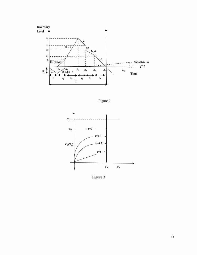
33

T

t2

z1

p1y

t1

Time (1-p1) x - λ

z2

B

Sales Returns

= αq2y T

Φ1 -λ

A1 A2 A3 A4 A3

Inventory

Level

-(-λ)

Φ - (1-p1) x

Φ – λ

-λ

-λ

z5

z4

z3

A5 A6

t3 t4 t5 t6

Figure 2

C0(Tp)

Cmax

C0

ϵ=0.1

ϵ=0.5

ϵ=1

ϵ=0

TM

TP

Figure 3

34

Table 2

Description Symbol Numerical 1

Numerical 2 Units

Production rate φ 2,00,000 1,50,000 units/ cycle

Screening cost during production

d1 0.5 0.6 $ / unit

Shortage cost cB 10 14 $ / unit / year

Screening rate x 1,75,200 1,00,000 units / year

Set-up cost C0 100 120 $ / cycle

Purchase cost c 25 30 $ / unit

Salvage cost v 16 20 $ / unit

Holding cost h 5 6 $ / unit / year

Table 3

T

Description Symbol Numerical 1

Numerical 2 Units

Defect proportion Α U ~ (0.4,0.6) U ~ (0.5,0.15)

Type-1 error proportion q1 U ~ (0.05,0.15) U ~ (0.2,0.8)

Type-1 error proportion q2 U ~ (0.1,0.3) U ~ (0.2,0.8)

Rework proportion R U ~ (0.5,0.7) U ~ (0.5,0.8)

Probability density function f(α) 1/(0.6 - 0.4) 1/(0.15 - 0.5)

Probability density function f(q1) 1/(0.3 - 0.1) 1/(0.8 - 0.2)

Probability density function f(q2) 1/(0.3 - 0.1) 1/(0.8 - 0.2)

Probability density function f(r) 1/(0.7 - 0.5) 1/(0.8 - 0.5)

Demand Rate λ 90,000 50,000 units / year

Shape Factor ϵ 0.2 0.3

Rework Rate φ1 80,000 40,000 units / cycle

Selling Price S 60 70 $ / unit

Screening Cost post production d2 0.6 0.7 $ / unit

Second Screening Cost d3 0.7 0.8 $ / unit

Type-I error Cost cr 10 12 $ / unit

Type-II error Cost ca 12 12 $ / unit

Rework Cost cW 8 9 $ / unit

Disposal Cost u 2 3 $ / unit

Maximum Set-Up Cost Cmax - - $ / cycle

Holding Cost during Rework h1 6 6 $ / unit

35

Table 4

Description Symbol Numerical 1 Numerical 2 Units

Order size y* 1,648 701 units/cycle

Backorder Quantity B* 267 109 units/cycle

Expected total profit per unit time E [ Z*(y, B)] 30,55,994 18,60,999 $/year

Cycle Length T* 6.55 4.94 Days

Table 5

Description Symbol Numerical 1 Numerical 2 Units

One way Inspection E [ Z*(y, B)] 30,39,578 18,10,119 $ / year

Two way Inspection E [ Z*(y, B)] 30,55,994 18,60,999 $ / year

Table 6

ϵ Tp* y* B* T* E[Z*(y,B)] % Loss

0.1 4.12 2,258.45 366.89 8.98 30,54,899.54 -25.05

0.2 3.01 1,648.97 267.88 6.55 30,55,994.14 -25.09

0.3 2.10 1,149.54 186.74 4.57 30,56,944.69 -25.13

0.4 1.38 756.22 122.85 3.01 30,57,746.91 -25.17

0.5 0.84 461.71 75.01 1.84 30,58,400.44 -25.19

0.6 0.47 255.16 41.45 1.01 30,58,909.70 -25.21

0.7 0.46 251.86 41.64 1.01 30,60,737.84 -25.29

0.8 0.09 47.16 7.66 0.19 30,59,541.11 -25.24

Table 7

α y* B* T* E.T.C.U.* E.T.R.U.* E[Z*(y,B)]

0.01 1,681.62 272.75 6.79 23,07,399.23 54,04,698.80 30,97,299.57

0.03 1,664.67 270.26 6.67 23,37,406.30 54,14,210.53 30,76,804.23

0.05 1,648.98 267.88 6.55 23,67,883.41 54,23,877.55 30,55,994.14

0.07 1,634.43 265.60 6.44 23,98,841.05 54,33,703.70 30,34,862.66

0.09 1,620.97 263.41 6.34 24,30,289.94 54,43,692.95 30,13,403.01

Table 8

q1 y* B* T* E.T.C.U.* E.T.R.U.* E[Z*(y,B)]

0 1,648.97 267.88 6.55 23,58,548.20 54,23,877.55 30,65,329.35

0.01 1,648.98 267.88 6.55 23,67,883.41 54,23,877.55 30,55,994.14

0.02 1,648.97 267.88 6.55 23,77,218.61 54,23,877.55 30,46,658.94

0.03 1,648.97 267.88 6.55 23,86,553.82 54,23,877.55 30,37,323.74

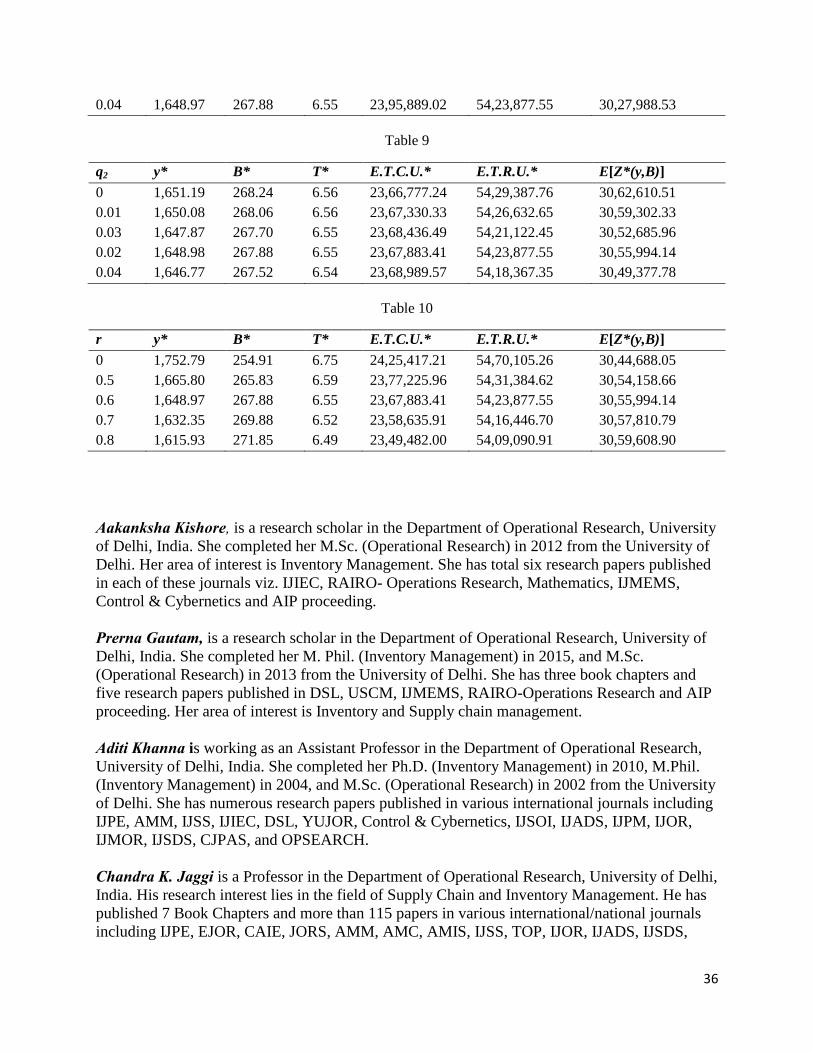
36

0.04 1,648.97 267.88 6.55 23,95,889.02 54,23,877.55 30,27,988.53

Table 9

q2 y* B* T* E.T.C.U.* E.T.R.U.* E[Z*(y,B)]

0 1,651.19 268.24 6.56 23,66,777.24 54,29,387.76 30,62,610.51

0.01 1,650.08 268.06 6.56 23,67,330.33 54,26,632.65 30,59,302.33

0.03 1,647.87 267.70 6.55 23,68,436.49 54,21,122.45 30,52,685.96

0.02 1,648.98 267.88 6.55 23,67,883.41 54,23,877.55 30,55,994.14

0.04 1,646.77 267.52 6.54 23,68,989.57 54,18,367.35 30,49,377.78

Table 10

r y* B* T* E.T.C.U.* E.T.R.U.* E[Z*(y,B)]

0 1,752.79 254.91 6.75 24,25,417.21 54,70,105.26 30,44,688.05

0.5 1,665.80 265.83 6.59 23,77,225.96 54,31,384.62 30,54,158.66

0.6 1,648.97 267.88 6.55 23,67,883.41 54,23,877.55 30,55,994.14

0.7 1,632.35 269.88 6.52 23,58,635.91 54,16,446.70 30,57,810.79

0.8 1,615.93 271.85 6.49 23,49,482.00 54,09,090.91 30,59,608.90

Aakanksha Kishore, is a research scholar in the Department of Operational Research, University

of Delhi, India. She completed her M.Sc. (Operational Research) in 2012 from the University of

Delhi. Her area of interest is Inventory Management. She has total six research papers published

in each of these journals viz. IJIEC, RAIRO- Operations Research, Mathematics, IJMEMS,

Control & Cybernetics and AIP proceeding.

Prerna Gautam, is a research scholar in the Department of Operational Research, University of

Delhi, India. She completed her M. Phil. (Inventory Management) in 2015, and M.Sc.

(Operational Research) in 2013 from the University of Delhi. She has three book chapters and

five research papers published in DSL, USCM, IJMEMS, RAIRO-Operations Research and AIP

proceeding. Her area of interest is Inventory and Supply chain management.

Aditi Khanna is working as an Assistant Professor in the Department of Operational Research,

University of Delhi, India. She completed her Ph.D. (Inventory Management) in 2010, M.Phil.

(Inventory Management) in 2004, and M.Sc. (Operational Research) in 2002 from the University

of Delhi. She has numerous research papers published in various international journals including

IJPE, AMM, IJSS, IJIEC, DSL, YUJOR, Control & Cybernetics, IJSOI, IJADS, IJPM, IJOR,

IJMOR, IJSDS, CJPAS, and OPSEARCH.

Chandra K. Jaggi is a Professor in the Department of Operational Research, University of Delhi,

India. His research interest lies in the field of Supply Chain and Inventory Management. He has

published 7 Book Chapters and more than 115 papers in various international/national journals

including IJPE, EJOR, CAIE, JORS, AMM, AMC, AMIS, IJSS, TOP, IJOR, IJADS, IJSDS,

37

DSL, YUJOR etc. He is a reviewer of more than 25 International/National journals. He has

guided 10 Ph. D. and 20 M. Phil. in Operations Research. He is Ex-Editor-in-Chief of IJICM,

Associate Editor of IJSAEM, Springer, and on the Editorial Board of the IJSS: Operations &

Logistics, IJSOI, AJOR, IJECBS, JASR, AJBAS.