A7_278

13th World Congress in Mechanism and Machine Science, Guanajuato, México, 19-25 June, 2011 A7_278

1

Isotropic Design of a 2 dof Parallel Kinematic Machine with a Translational

Workpiece Table

H. A. Moreno

* J. A. Pamanes

†

Technical University of Madrid Autonomous University of Coahuila

Madrid, Spain Torreon, Mexico

Abstract—Parallel Kinematic Machines (PKMs)

usually have the disadvantage of a reduced workspace.

This problem can be solved by adding a moving table

that relocates the workpiece for the PKM. In this paper

we present the isotropic design of a 2 degrees of freedom

PKM that works in cooperation with a moving table. For

the analysis we used the condition number of the

Jacobian Matrix of the whole kinematic chain (PKM-

table). This work reveals the benefits of using a

performance index, which considers the kinematics of

both components together and not separately. Keywords: Kinematic redundancy, Isotropic design, Condition

number.

I. Introduction

Although PKMs have interesting features for

machining applications, in many cases they do not have

sufficient workspace for machining large workpieces.

This handicap, however, can be overcame by

incorporating a secondary cooperative manipulator to aid

the main one (the PKM) to achieve the task. The

secondary manipulator should continuously relocate the

work-piece to the main one in such a way that the

kinematic performance of the chain is enhanced. In this

paper, the isotropic design of a system with the

previously cited characteristics is presented.

The strategy in which a positional device is

incorporated to aid the main manipulator has been

applied in previous works. In one paper [1] the main

manipulator was redundant, and the secondary was non-

redundant. Both manipulators cooperate to achieve a

welding task: the main one (right hand) moves the

welding torch and the positioner (left hand) continuously

relocates the work-pieces.

In this paper, we present the isotropic design of a 2-

PRR type PKM that works in cooperation with a

translational table, see Figure 1.

Fig. 1. 2 dof PKM and translational table

The PKM presented here is termed 2 dof Orthoglide,

[2][3]. The 2 dof Orthoglide can be used for machining

applications such as milling.

On the other hand, the translational table moves the

workpiece in such a way that the Orthoglide’s end

effector is enabled to reach task points that could not be

reached otherwise. The translational table moves only in

one direction, even though the workspace is significantly

increased, as it will be demonstrated later.

In this paper we analyze the benefits of using a

kinematic performance index obtained from coupled

manipulator kinematics. In consequence, the optimal

configurations from the point of view of the condition

number are obtained regarding the Jacobian matrix of the

whole kinematic chain.

We consider three optimal configurations and analyze

errors corresponding to each, in order to numerically

Workpiece

Translational table

2 dof PKM

End Effector

Actuated

Prismatic Joint

*[email protected]

†[email protected]


2

2ρ

0

cr

0y

0x

A

B

C

1ρ

1θ

1y

1x

3ρ

0

cr

0y

0x

2ρ

1ρ

revealing and contrasting the PKM’s performance during

a task.

II. Preliminaries

The kinematic scheme of the 2 dof Orthoglide is

shown in Figure 2. As can be observed, the PKM is

composed of two actuated sliding blocks which are

coupled to the fixed frame by prismatic joints. On the

other hand, the blocks are connected to the links AC and

BC by the revolute joints A and B, respectively. Lastly,

such links are connected by the revolute joint C. All the

revolute joints are passives. The axes of the prismatic

joints are orthogonal.

Fig. 2. Kinematic scheme of the 2 dof Orthoglide.

Figure 3 shows a kinematic scheme of the Orthoglide

and the cooperative table with translational motion. We

name this system (Orthoglide and table) assisted PKM.

The direction of motion of the table is defined by the

angle 1θ . On the other hand,

1γ is half of the angle

between the sliding blocks movement axes. By

definition, for the Orthoglide we have 1 45γ = ° .

Fig. 3. Kinematic scheme of the 2 dof Orthoglide with the cooperative

table.

In the following, we consider lengths of bars AC and

BC as being 1mL = ; besides, we maintain the angle

1 45θ = ° , since the workspace reaches its maximum at

this value.

It can be observed in Figure 4 that the PKM’s

workspace oW is increased by incorporating a

cooperative table. If tl was the length of the largest

transversal line that the PKM is able to draw on the table,

then the assisted PKM’s workspace is given by :

3op o tW W l ρ= + ∆ with3 3max 3minρ ρ ρ∆ = − .

(a) (b)

Figure 4. Workspace of the 2 dof Orthoglide. (a) Without cooperative

table, (b) Assisted PKM

A. Kinematics of the assisted PKM

The joint and operational velocity vectors, ρ and t,

respectively, of a parallel manipulator are related as

follows:

At = Bρ& (1)

In (1), A and B are, respectively, the parallel and serial

Jacobian matrices, [4]. The entries of these matrices

depend on both the design variables and manipulator

pose.

For the Orthoglide without table, the joint velocity

vector is given by [ ]1 2

Tρ ρ=ρ& & & and the operational

velocity vector is [ ]Tcx cyr r=t & & . The scalars cxr& and

cyr&

are the orthogonal components of the position vector 0rc

(corresponding to point C) referred to a frame x0-y

0, (Fig.

1.) For the Orthoglide we have:

0

4

0

5

ˆ

ˆ

T

o T

=

rA

r (2)

1 4

2 5

ˆ ˆ0

ˆ ˆ 0

T

o T

=

r rB

r r (3)

1γ

1γ

2γ

3γ

4r̂

1̂r

2r̂

5̂r

3̂r

tl

m1.50 2 ≤≤ ρ

m1.50 3 ≤≤ ρ

m 11- 3 ≤≤ ρ


3

For the assisted PKM (Figure 3), the joint velocity

vector is given by [ ]1 2 3

Tρ ρ ρ=ρ& & & & and the operational

velocity vector is defined in the same way that the last

case. The corresponding Jacobian matrices are:

0

4

0

5

ˆ

ˆ

T

op T

=

rA

r (4)

1 4 3 4

2 5 3 5

ˆ ˆ ˆ ˆ0

ˆ ˆ ˆ ˆ0

T T

op T T

=

r r r rB

r r r r (5)

The symbol ^ on a vectorial term of these equations

designates unit vector. In matrices (4) and (5) the unit

vectors correspond to the position vectors associated with

PKM’s links, as shown in Figure 2. The velocity of point

C (end-effector) of the Orthoglide relative to the table is

obtained from Equation 1 as:

=t Jρ& (6)

where 1−=J A B .

On the other hand, since the assisted PKM can be

considered as a redundant one, the general solution of the

inverse kinematic problem is written as follows:

( )+ += + −ρ J t I J J z& (7)

The term +J t is the least norm solution of the inverse

kinematic problem. The expression ( )+−I J J z , is the

homogenous solution, which represents the projection of

z on the null space of J .

B. Singular configurations

It can be shown that matrix oA and

opA are singular

when vectors 4r and 5r (i.e. links AC and BC) are

parallel; in this case the PKM is on a parallel singularity.

Figure 5(a) show a configuration which corresponds to a

parallel singularity. It is possible to observe that the PKM

can not support any force perpendicular to links AC and

BC; consequently point C could be moved even if the

actuators are blocked. This situation is obviously

undesirable.

On the other hand, in (3) it can be observed that matrix

oB is singular when vectors 1r and

4r , or 2r and

5r ,

become orthogonal. In this case the PKM is on a serial

singularity. In this situation, the PKM is not able to move

its end-effector.

Fig. 5. Parallel (a) and serial (b) singularities.

When matrix opB is rank-deficient the PKM cannot

control its end-effector. Figure 5(b) shows a serial

singularity at which the PKM is unable to move point C;

in this case the relative movement, between point C and

the table, only can be in parallel direction to the table axis

of motion.

Note that vector 3r does not have any influence over

matrix opA . On the other hand, even though some entries

of matrix opB depend on

3r , this vector cannot produce a

rank loss.

III. Kinematic Performance Index

There are several works on indexes that evaluate the

kinematic performance of serial manipulators, for

example, those introduced in [5],[6],[7]. However, the

extension of those indexes for their application in parallel

manipulators is not immediate because of the existence of

two Jacobian matrices, each of them with a different

function in the PKM kinematic model. Therefore, the

performance evaluation through an arbitrary index used

in serial manipulators could produce undesirable results

in parallels.

In this article, the condition number is used as a

performance index, since it can be efficiently applied to

both serial and parallel manipulators [6].

The condition number of the Jacobian matrix is an

interesting index for evaluating the PKM kinematic

performance. This index measures the uniformity of the

velocities and forces distribution that could develop end-

effector in all directions [8], this feature is a priority for

tasks such as machined processes [9, 10].

Besides, the condition number limits the error

propagation from the joint velocities to the end-effector

velocities. In consequence, it is necessary to maintain

that number in its lowest possible value for the purpose

of preserving an adequate precision level of the

manipulator’s movements. The condition number of a

matrix J is defined as

m

M

λλ

κ =(J) ( 8 )

A, B

C

C A

B

(a) (b)


4

where Mλ and

mλ are maximum and minimum

singular values of J, respectively. The minimum value

that could reach κ(J) is 1. When one configuration

reaches this ideal value, it is said that the configuration is

isotropic. On the other hand, κ(J) becomes infinite when

the PKM is in a singular configuration.

The condition number of the Othoglide κo= κ(Jo), is

calculated from the next Jacobian matrix:

1

o o o

−=J A B ( 9 )

On the other hand, the condition number of the assited

PKM κop= κ(Jop), is determined by the following

Jacobian matrix:

1

op op op

−=J A B (10)

The matrixes A and B from the equation (9) and (10)

are defined in equations (2) to (5).

IV. Isotropic Design and Configurations

Isotropic configurations are those whose condition

number is equal to the unit. In this kind of configuration,

the PKM is capable of displacing the end-effector in the

same extent in all directions. If a PKM is capable of

reaching an isotropic configuration, it is called isotropic.

Two degree of freedom planar manipulators are an

important type of robotic mechanism that can follow an

arbitrary planar curve. Because of their usefulness in

applications, these mechanisms have drawn the attention

of researches who have investigated their workspace and

design [2, 3, 13]. The robots taken into consideration

were not redundant in those works. In [14] an analysis

was developed to determine the isotropic design of a n-

axis planar serial manipulator, this manipulato was

intended for positioning the end-effector in the x-y plane.

In that work, Angeles pointed out that isotropic

conditions could be achieved in several ways. Because

the entries of the Jacobian matrices (4) and (5) are based

on five unit vectors, there are different ways to determine

an isotopic configuration.

The Jacobian matrices can be expressed in terms of

five angles that correspond to the unit vectors. For

simplicity and regarding the PKM structure, we choose

only three angles that characterize the design and position

of the assisted PKM. Those are 1γ ,

2γ , and 3γ , and

were previously shown in Fig 4. Those angles describe

the orientation of vectors 1r ,

2r , 4r and

5r with respect

the motion axis of the table.

Regarding the angles 1γ ,

2γ and 3γ , the Jacobian

matrices (4) and (5) become:

2 2

3 3

sin( ) cos( )

sin( ) cos( )op

γ γγ γ

− =

A (11)

1 2 2

1 3 3

0 cos( ) cos( )

cos( ) 0 cos( )op

γ γ γγ γ γ

− − = − −

B (12)

hence, the Jacobian matrixopJ is set in the following

way:

2 1 3 3 1 2

2 1 3 3 1 2 2 3

cos( )cos( ) cos( ) cos( ) 0

sin( ) cos( ) sin( ) cos( ) sin( )op d

γ γ γ γ γ γγ γ γ γ γ γ γ γ

− − − = − − − − +

J

(13)

where 2 31/ sin( )d γ γ= + .

If we let K be defined in the following way :

T

op op=K J J (14)

opJ becomes isotropic when [15 ] :

τ=K I (15)

the entries of K are given by

11 12

21 22

k k

k k

=

K

where: 2 2 2 2 2

11 3 1 2 2 1 3cos( ) cos( ) cos( ) cos( )k d γ γ γ γ γ γ = − + − 2 2 2 2 2 2

22 2 3 3 1 2 2 1 3sin( ) sin( ) cos( ) sin( ) cos( )k d γ γ γ γ γ γ γ γ = + + − + − 2 2 2

12 2 1 3 2 3 1 2 3cos( )cos( ) sin( ) cos( )cos( ) sin( )k d γ γ γ γ γ γ γ γ = − − −

12 21k k=

(16 a-d)

The isotropic conditions from (15) are

12 21 0k k= = and 11 22k k τ= = . It is easy to observe from

(16c), d that 12k and

21k become zero when 2 3γ γ= for

any value of 1γ . On the other hand, if we regard

2 3γ γ=

then the equality 11 22k k τ= = becomes :

2 2 2 2

2 2 1 2 22 cos( ) sin( ) cos( ) sin(2 )γ γ γ γ γ − − = (17)

resolving for 1γ :

2 21 2

tan(2 )sin(2 )= +acos

2

γ γγ γ

±

(18)


5

Fig. 6. Isotropic designs.

In Fig. 6 the values of 1γ and

2 3γ γ= which provide

the isotropic design are shown. Fig. 6 shows that there

are several isotropic designs and their corresponding

poses. It is very important to note that when 2 0ºγ = the

links AB and BC are parallel and the PKM assumes a

singular configuration of parallel type (Fig. 5a). Even

though the Jacobian matrix (13) remains isotropic when

2γ is close to zero, the PKM loses its ability to move in

the 0y direction. Therefore it is not advisable to choose

design variables when 2γ is close to zero.

In the following subsections we use the results derived

in preceding paragraphs, and obtain from (18) an

isotropic configuration for the Orthoglide (it means

1 45ºγ = ). Furthermore, we derive an isotropic design

where the motion axes of the actuated joints are

symmetrically situated. We compare its performance

regarding the velocity error in the isotropic configuration.

Case 1: Orthoglide Isotropic Configuration

The Orthoglide isotropic configuration is shown in

Fig. 6. In this configuration, the velocity cxr& is directly

proportional to the joint velocity2ρ& , therefore the

velocity errors in the 0x direction are only a product of

velocity errors in the actuator associated to2ρ& , but not of

two actuators at the same time. The same occurs in the

case of cyr& , whose velocity is given by

1ρ& .

On the other hand, the PKM has not only an isotropic

configuration, there are a set of isotropic configurations

that correspond to a continuum of workspace points

defined by a 45 ° straight line segment with respect to

the frame x0-y

0 [15]. When the PKM’s end-effector

reaches points over this line 1oκ = ; but, even though the

singular values that correspond to one point in the line

are equal among them, the magnitudes of those values

change at different points in the line.

When the Orthoglide, under one configuration such as

1oκ = , is required to work with a moving table, it is

observed that κop ≠ 1, therefore this assisted PKM

configuration is not isotropic. In this configuration, the

Jacobian matrix of the whole kinematic chain is given by:

(1)

0.7071 0.7071 0

0.7071 0.7071 1op

− = − − −

J , (19)

from which 1.4142opκ = is obtained.

Fig. 7. Orthoglide isotropic configuration

Case 2: Assisted PKM Isotropic Configuration

The minumum condition number that is obtained

inside the PKM’s workspace is 1opκ = . In Fig. 8, the

configuration corresponding to this value is shown. In

this configuration, the robot is Isotropic.

In the isotropic configuration the Jacobian is given by:

(2)

0.9127 0.9127 0

0.5771 0.5771 1op

− = − − −

J (20)

Fig. 8. Assisted PKM isotropic configuration.

Case 3: Isotropic design of the assisted PKM

In Fig. 9, the isotropic design of the PKM can be seen

in an isotropic configuration. In this case the Jacobian

matrix results in:

(3)

0.8660 0.8660 0

0.5 0.5 1op

− = − −

J (21)

In this case 1opκ = is obtained.

1γ

1γ (deg)

1γ

2 3γ γ= (deg)

Isotropic

continuuum


6

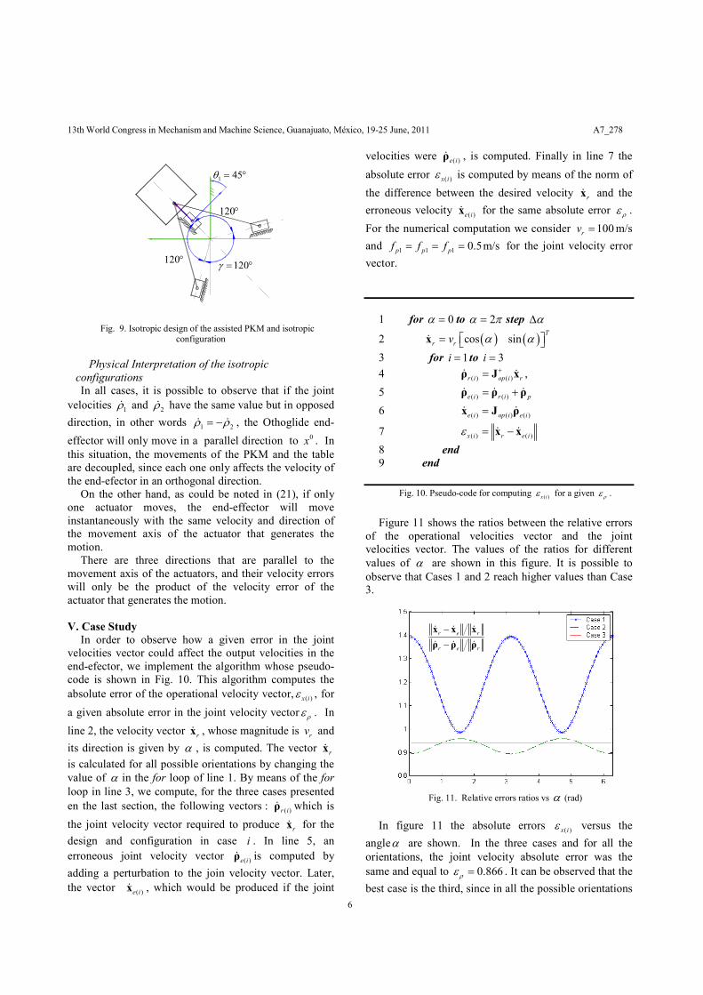
120γ = °

120°

120°

1 45θ = °

Fig. 9. Isotropic design of the assisted PKM and isotropic configuration

Physical Interpretation of the isotropic

configurations

In all cases, it is possible to observe that if the joint

velocities 1ρ& and

2ρ& have the same value but in opposed

direction, in other words 1 2ρ ρ= −& & , the Othoglide end-

effector will only move in a parallel direction to 0x . In

this situation, the movements of the PKM and the table

are decoupled, since each one only affects the velocity of

the end-efector in an orthogonal direction.

On the other hand, as could be noted in (21), if only

one actuator moves, the end-effector will move

instantaneously with the same velocity and direction of

the movement axis of the actuator that generates the

motion.

There are three directions that are parallel to the

movement axis of the actuators, and their velocity errors

will only be the product of the velocity error of the

actuator that generates the motion.

V. Case Study

In order to observe how a given error in the joint

velocities vector could affect the output velocities in the

end-efector, we implement the algorithm whose pseudo-

code is shown in Fig. 10. This algorithm computes the

absolute error of the operational velocity vector,( )x iε , for

a given absolute error in the joint velocity vector ρε . In

line 2, the velocity vector rx& , whose magnitude is

rv and

its direction is given by α , is computed. The vector rx&

is calculated for all possible orientations by changing the

value of α in the for loop of line 1. By means of the for

loop in line 3, we compute, for the three cases presented

en the last section, the following vectors : ( )r iρ& which is

the joint velocity vector required to produce rx& for the

design and configuration in case i . In line 5, an

erroneous joint velocity vector ( )e iρ& is computed by

adding a perturbation to the join velocity vector. Later,

the vector ( )e ix& , which would be produced if the joint

velocities were ( )e iρ& , is computed. Finally in line 7 the

absolute error ( )x iε is computed by means of the norm of

the difference between the desired velocity rx& and the

erroneous velocity ( )e ix& for the same absolute error ρε .

For the numerical computation we consider 100rv = m/s

and 1 1 1 0.5m/sp p pf f f= = = for the joint velocity error

vector.

1 for 0α = to 2α π= step α∆

2 ( ) ( )cos sinT

r rv α α= x&

3 for 1i = to 3i =

4 ( ) ( )r i op i r

+=ρ J x& & ,

5 ( ) ( )e i r i p= +ρ ρ ρ& & &

6 ( ) ( ) ( )e i op i e i=x J ρ&&

7 ( ) ( )x i r e iε = −x x& &

8 end

9 end

Fig. 10. Pseudo-code for computing ( )x iε for a given ρε .

Figure 11 shows the ratios between the relative errors

of the operational velocities vector and the joint

velocities vector. The values of the ratios for different

values of α are shown in this figure. It is possible to

observe that Cases 1 and 2 reach higher values than Case

3.

Fig. 11. Relative errors ratios vs α (rad)

In figure 11 the absolute errors ( )x iε versus the

angleα are shown. In the three cases and for all the

orientations, the joint velocity absolute error was the

same and equal to 0.866ρε = . It can be observed that the

best case is the third, since in all the possible orientations

r e r

r e r

−

−

x x x

ρ ρ ρ

& & &

& & &


7

it always preserves the lowest value of absolute error

( )x iε . On the other hand, the best second case is case 2. It

is possible to observe that cases 2 and 3 are closer than

cases 2 and 1. In conclusion, it is possible to observe that

the third case was the least affected by the errors in the

joint velocity vector.

0 1 2 3 4 5 60.95

1

1.05

1.1

1.15

1.2

1.25

Case 1

Case 2

Case 3

Fig. 11. Absolute errors vs α (rad)

VI. Conclusions

In this paper we presented the isotropic design of a 2

dof PKM that works in cooperation with a translational

table. It was shown that the workspace is directly

proportional to the range of motion of the translational

table, and can be significantly amplified when the table is

added. For the kinematic analysis we used the condition

number of the Jacobian Matrix of the whole kinematic

chain. Three angles were used to characterize the design

and position of the assisted PKM in order to simplify the

analisys. A Jabobian matrix in function of these angles

was derived. By means of this analysis, we found the

geometric conditions to attain isotropic designs and

configurations. Three optimal designs were considered in

order to make a numerical study of the velocity errors

corresponding to each. In all cases, it is possible to

observe that if the PKM’s joint velocities 1ρ& and

2ρ&

have the same value but in opposed direction, in other

words 1 2ρ ρ= −& & , the PKM end-effector will only move

in a parallel direction to 0x . In this situation, the

motions of the PKM and the table are decoupled, since

each one only affects the velocity of the end-efector in an

orthogonal direction. A symmetric design was found, and

it was observed that if only one actuator moves, the end-

effector will move instantaneously with the same velocity

and direction of the movement axis of the actuator that

generates the motion. There are three directions that are

parallel to the movement axis of the actuators, and their

velocity errors will only be the product of the velocity

error of the actuator that generates the motion. It was

shown that the Orthoglide’s isotropic configuration is not

valid when it works in cooperation with a translational

table. This work revealed the benefits of using a

performance index, which considers the kinematics of

both components together and not separately. In this

paper we presented the isotropic design of a mechanical

system for a real aplication, the analsys provides

meaningful results at practical and conceptual levels.

References

[1] Hemmerle J.S., Prinz F.B, “Optimal Path Placement for

Kinematically Redundant Manipulators,” Proceedings of the 1991 IEEE International Conference of Robotics and Automation, pp.1234-1243.

[2] Majou F., Wenger P., Chablat D., “Design of 2-DOF Parallel

Mechanisms for Machining Applications,” Advances in Robot Kinematics: Theory and Applications; Kluwer Academic

Publishers. Edited by J. Lenarcic and F. Thomas; pp. 319-328,

2002. [3] Wenger P., Gosselin C., Chablat D. “A comparative study of

parallel kinematic architectures for machining applications,” 2nd

Workshop on Computational Kinematics, Seoul South Korea; 2001. [4] Gosselin C., Angeles J., “Singularity analysis of closed-loop

kinematic chains,” Proceedings of the 1990 IEEE International

Conference of Robotics and Automation. [5] Yoshikawa T., “Manipulability of Robotics Mechanisms,”

Robotics Research: The second International Symposium, pp.439-

446, 1984. [6] Angeles J., López-Cajún C., “Kinematic Isotropy and

Conditioning Index of Serial Robotic Manipulators,” Int. J.

Robotics Research; 11 (6), pp. 560-571 (1992). [7] Chiu, S. L., “Task compatibility of manipulators postures,” Int.

J. Robotics Research, 7 (5), 13-21, 1988.

[8] Salisbury J.K., Craig J. J., “Articulated hands: force and kinematic issues,” The Int. J. of Robotic Research, vol. 1(1), pp. 4-17, 1982.

[9] Chablat D., Wenger P., “Architecture Optimization of a 3-DOF

Parallel Mechanism for Machining Applications, the Orthoglide,” IEEE Transactions on Robotics and Automation, vol. 19(3), pp

403-410, juin 2003.

[10] Huang T., Whitehouse D., “Local dexterity, optimal architecture and optimal design of parallel machine tools,” Ann.

CIRP, vol. 47, no. 1, pp. 347–351, 1998.

[11] Zanganeh K. E., Angeles J., “Kinematic isotropy and the optimum design of parallel manipulators,” Int. J. Robot. Res., vol.

16, no. 2, pp. 185–197, 1997.

[12] Baron L., Bernier G., “The design of parallel manipulators of star topology under isotropic constraint,” Proc. DETC ASME,

Pittsburgh, PA, 2001. [13] Tian Huang, Meng Li, Zhanxian Li, Derek G. Chetwynd, and

David J. Whitehouse, “Optimal Kinematic Design of 2-DOF

Parallel Manipulators With Well-Shaped Workspace Bounded by a Specified Conditioning Index,” IEEE Transactions On Robotics

And Automation, Vol. 20, No. 3, June 2004 pp 538 543.

[14] Jorge Angeles, “The Design of Isotropic Manipulator Architectures in the presence of Redundancies,” The International

Journal of Robotics Research. Vol. 11. No. 3. June 1992. pp. 196-

201. [15] Angeles J., Fundamentals of robotic mechanical systems,

Springer-Verlag, New York. 3rd ed., 2007.

A7_278

Documents

Transcript of A7_278