124 IEEE TRANSACTIONS ON COMPONENTS, HYBRIDS, AND MANUFACTURING TECHNOLOGY, VOL. 14. NO. 1, MARCH 1991

A Weibull Model to Characterize Lifetimes of Aluminum Allov Electrical Wire Connections

Carol F

A bstract-Samples of 12 gauge aluminum alloy electrical conductor wire, including aluminum 1350 and one 8000 series alloy, and three different connector torques were tested to lo00 cycles, using an acceler- ated test method which is independent of commercially available connec- tors. A Weibull probability model was fitted to the number of cycles to failure, for each of the torques for each alloy. For all groups, 6 (Weibull shape parameter, describing the spread in observed connection lifetimes) was in the range of 1-2. The parameter a (location parameter, descrih- ing the characteristic connector lifetime) increased as connector torque increased, and had a value characteristic of the alloy used. Assuming a Weibull model for failure of electrical connectors for aluminum wire, acceptance plans were developed to discriminate between alloys with different characteristic lifetimes. Experiments confirmed the ability of the acceptance plans to clearly discriminate between known alloys.

I. INTRODUCTION ONNECTABILITY tests to evaluate suitability of various C alloys for electrical conductors usually take the form of

connecting several samples of wire together in series and sub- jecting them to cycles of on/off current. The current used is much higher than would be encountered by the wire in normal use, and hence, these are accelerated tests, giving failures much earlier than in normal use. Failure of the connection is usually indicated by observation of a predetermined temperature that is much above ambient temperature.

The currently used acceptance test for aluminum branch cir- cuit electrical conductor wire runs for 500 cycles of 3-1/2 h on and 112 h off, thus taking nearly 12 weeks to evaluate an alloy. Connections are made using commercial connectors which are no longer manufactured, and therefore, are subject to shelf life aging problems [4]. An hypothesis first put forward by Battelle Columbus Laboratories [23] and later tested at Alcan [20], was used to develop a test of shorter duration. Using this accelerated method, tests were run, using 96 samples of 12 gauge uninsu- lated aluminum electrical conductor wire, 48 each of two alloys: AA-1350’ (formerly Electrical Conductor grade) and AA-8076, a CSA certified, UL listed ACM conductor alloy, sold under the trade name NUAL.TM AA-8076 alloy wire is known to have superior connectability and lifetime. These two alloys were chosen as those with extremes of connectability characteristics. Within each alloy, wires were connected with one of 3 different torques (0.8, 1.0, and 1.2 N-m). Thus there were 6 alloy-torque groups, each with 16 replicates. The number of cycles to failure was recorded.

Manuscript received April 1, 1990; revised October 26, 1990. This paper was presented at the 36th IEEE Holm Conference on Electrical Contacts, Montreal, P.Q., Canada, August 20-24, 1990.

The author is with the Kingston Research and Development Centre, Alcan International Ltd., Kingston, Ont., Canada K7L 5L9.

fEEE Log Number 9041694. Aluminum alloys are designated as AA-nnnn, by the Aluminum Associa-

tion. NUAL registered trademark of Alcan Aluminium Ltd. TM

Joyce

This paper uses a Weibull model to predict the number of cycles to failure for the wire, and then develops acceptance plans to discriminate between alloys with different Weibull characteris- tic lifetime parameters.

11. THE WEIBULL DISTRIBUTION

In 1951, Weibull [24], a Professor of Applied Physics at Royal Institute of Technology in Stockholm, Sweden, published a paper describing a probability distribution based on the sim- plest mathematical function to describe the probability of a chain breaking (due to failure of an individual link), as the load ( x ) on the chain increases. The “weakest link” model may be applied to many life testing and reliability situations. The probability of an item lasting to load x , or time x , is the cumulative form of the Weibull probability distribution, given by

x--y B F ( x ) = 1 - e - ( , ) , x r y , a > O , P > O (1)

where

x random variable, F( x) cumulative probability of failure or cumulative fre-

quency of values of x, (Y scale parameter (or characteristic life = 63.2 per-

centile),’ 6 shape parameter, y location parameter.

This equation may be transformed to a linear form:

Equation (2) is a linear function of l n ( x - y), so when In In (1 /( 1 - F( x ) ) is plotted against In ( x - y), data from a Weibull distribution will fall on a straight line with slope = 0, and intercept - P . In ( a ) . This is the basis for Weibull probability plotting scales. Fig. 1 shows various plots of Weibull distribu- tions, for the same value of a , and different values of 0.

This distribution has been used since the 1930’s, to describe particle size distributions [l], [8], [9], where it is known as the Rosin-Rammler distribution, after the individuals who proposed it as a model to describe the size distribution of fine powdered coal [18]. Harris suggests acceptance of the Rosin-Rammler distribution as the preferred method for representing pulveriza- tion data as an international standard for coal preparation and mineral processing applications [9].

Weibull’s name became associated with the distribution be- cause he used it as an empirical model to describe a variety of physical properties [24], [25]. Since then, the distribution has been used to empirically model many and diverse processes,

When ( x - y) = a , (1) becomes F ( x ) = 1 - e - ’ = 0.632, for all 6.

0048-6411/91/0300-0l24$01.00 0 1991 IEEE

JOYCE: MODEL TO CHARACTERIZE LIFETIMES OF ELECTRICAL WIRE CONNECTIONS 125

1 1 . 0 . t‘, 0

0 - x w -

0

0

0

Fig. 1. Plots of Weibull distributions.

especially lifetimes of systems subjected to stress [3], [5], [6], [lo], [12], [13], [19], [22]. Thus it is appropriate to consider a Weibull model to describe the lifetimes of single strand 12 gauge aluminum conductor wire connections.

111. INTERPRETATION OF THE WEBULL PARAMETERS The Weibull distribution is an empirical model that fits many

types of observed data very well, where other or theoretical mathematical models do not exist. The form of the distribution is really a family of curves, and a system behaves differently depending on values of the parameters. Values of the parameters a! and 0 have been assigned physical significance: a indicating an average or characteristic value or lifetime, and P indicating the dispersion of the failures. In Fig. 1, all the curves have a = 1; as a! increases, the curves would be displaced along the x axes.

> 1, the rate of failure increases with time (or stress), which is intuitively a reasonable model for an aging or stressed system. When P < 1, failures are due to “infant mor- tality” or manufacturing defects, and the failure rate decreases with time. When = 1, the rate of failure is constant over time. It has been suggested [21] that in any Weibull distribution, early failures are mechanical, due to physical defects, and delayed

When

failures are electrical or chemical, and are usually associated with component wear.

For specific values of P, the Weibull distribution may be known by other names [21]. When 0 = 1, the Weibull distribu- tion is an exponential one, and the rate of failure is constant over time. When P = 2, it is a Rayleigh distribution, which deals with errors in a two-dimensional grid. When P = 3.25, it is (approximately) a normal distribution.

If the data plotted on a Weibull scale appear to be a bent line, or two lines intersecting, this could be due to two different failure modes, with different values for P. The lower P values are consistent with catastrophic or sudden failures and the higher

values indicate wear out or delayed failures. Examples of dual failure modes have been reported for electron tubes [Il l , and gas generators [ 141. Proportions of data in each of the distribu- tions may be estimated by the method of moments [17] or maximum likelihood methods [5].

The parameter y indicates a minimum lifetime. If y < 0, it means that the item failed some time before going into service, or experienced shelf life failure. y = 0 implies the earliest failure could be at time 0, which is normally encountered. Cases where y > 0 are ones where there is some physical constraint where there could be absolutely no occurrences below this minimum value. For example, for the case of particle sue

126 IEEE TRANSACTIONS ON COMPONENTS, HYBRIDS, AND MANUFACTURING TECHNOLOGY, VOL. 14, NO. 1 , MARCH 1991

distributions, small particles may be either undetectable or phys- ically not present in the sample. Also, in the case of multiple failure modes, there may be a mode of failure which cannot occur until a minimum time has elapsed [ 1 I], [ 141.

IV. ESTIMATION OF WEIBULL PARAMETERS Estimates of a and 0 may be obtained from a plot of

cumulative probability distribution data on Weibull scales. Least-squares estimates of the parameters for (2 ) may be ob- tained by fitting the transformed data to a linear function, and then transforming again to get a and 0 estimates. Least-squares estimates of a and 0 may be obtained directly by fitting observed data to (I), but results are nearly impossible to obtain without reasonable starting values. Starting values for the least- squares fit may be obtained from the linear fit to ( 2 ) . This method is quite satisfactory for situations where failure informa- tion is available for all the data-for example, when all speci- mens have failed, or in the case of particle size distribution data, when all of the sample may be classified into intervals for the cumulative probability distribution.

In many cases total failure of test families or complete classi- fication is not possible. However, maximum likelihood (ML) methods use information about failed and continuing items, and is the appropriate method to estimate parameters in these situa- tions. Observations for which complete data is not known are censored data, and the termination time of the test is the censoring time. ML methods may be used then to estimate parameters for a life distribution, using lifetime data for which all items have not failed (censored data), and for which the continuing items have different lifetimes (multiply censored data). Methods for estimating Weibull parameters from multiply cen- sored data using ML methods, are outlined in Nelson's text and his monograph from the American Society of Quality Control [W, V61.

ML parameter estimates are those which are most likely to be the ones to describe the distribution from which the observed data are obtained. A Weibull likelihood function for multiply censored data incorporates information about the Weibull distri- bution, the observed failures, lifetimes of continuing items, and parameters a and 0. The log-likelihood function is maximized when the first derivative is zero. When the first derivative is zero, the second derivative (with respect to each of the parame- ters) represents the change in ML with respect to each of the parameters-i.e., the variance-covariance matrix for the param- eter estimates.

The ML method, therefore, provides the best way of estimat- ing the most likely values of the parameters of the Weibull distribution, given a set of observed censored data. (With com- plete uncensored data, the ML estimates are nearly equal to the least-squares estimates.) The ML method also provides an esti- mate of the variability of the estimates, from which confidence intervals for the parameters may be obtained. The log-likelihood function for the Weibull distribution (with parameters a , p) , for a sample of n units with r failures is given by

-?'("" a (3)

where E' runs over all failed items, CL runs over all unfailed

items, and ti = lifetime. i i

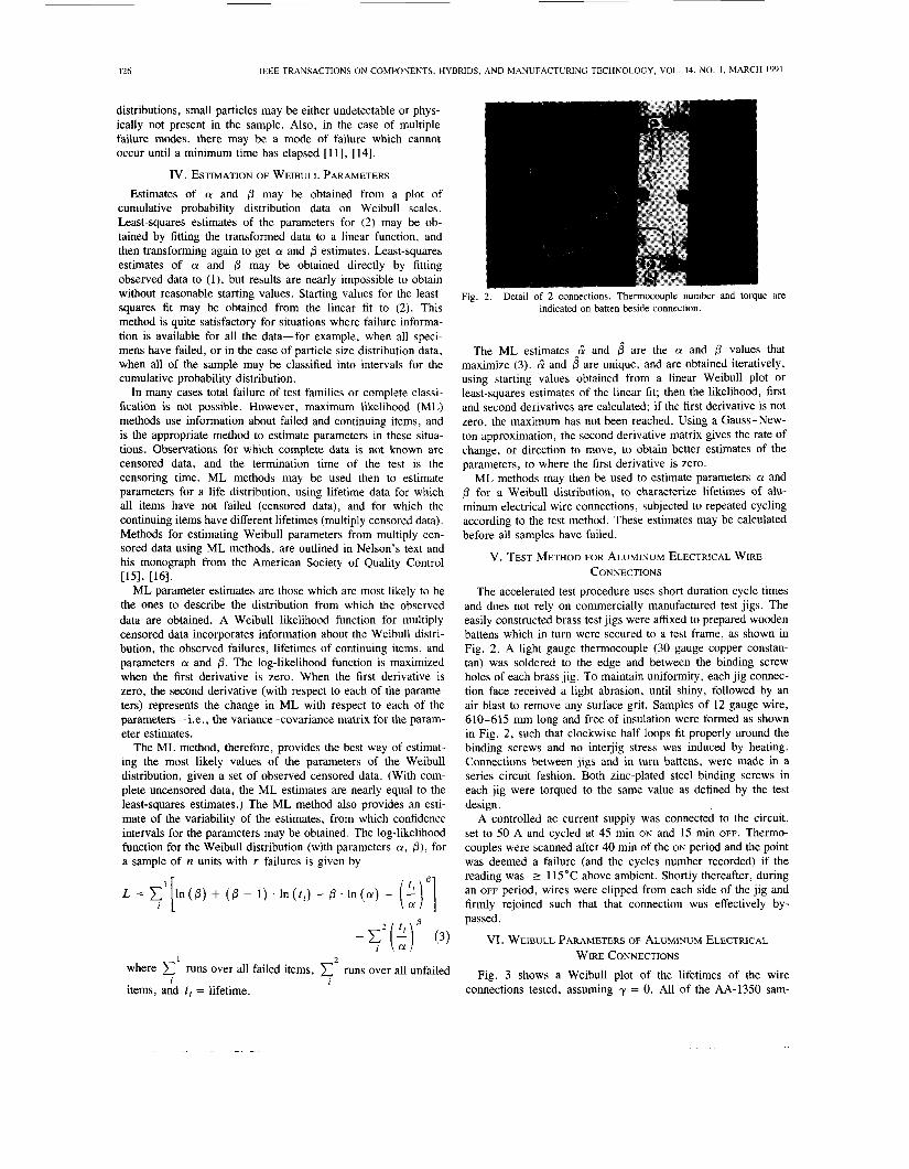
Fig. 2. Detail of 2 connections. Thermocouple number and torque are indicated on batten beside connection.

The ML estimates A& and are the a and 0 values that maximize (3). 13 and 0 are unique, and are obtained iteratively, using starting values obtained from a linear Weibull plot or least-squares estimates of the linear fit; then the likelihood, first and second derivatives are calculated; if the first derivative is not zero, the maximum has not been reached. Using a Gauss-New- ton approximation, the second derivative matrix gives the rate of change, or direction to move, to obtain better estimates of the parameters, to where the first derivative is zero.

ML methods may then be used to estimate parameters a and for a Weibull distribution, to characterize lifetimes of alu-

minum electrical wire connections, subjected to repeated cycling according to the test method. These estimates may be calculated before all samples have failed.

V. TEST METHOD FOR ALUMINUM ELECTRICAL WIRE CONNECTIONS

The accelerated test procedure uses short duration cycle times and does not rely on commercially manufactured test jigs. The easily constructed brass test jigs were affixed to prepared wooden battens which in turn were secured to a test frame, as shown in Fig. 2 . A light gauge thermocouple (30 gauge copper constan- tan) was soldered to the edge and between the binding screw holes of each brass jig. To maintain uniformity, each jig connec- tion face received a light abrasion, until shiny, followed by an air blast to remove any surface grit. Samples of 12 gauge wire, 610-615 mm long and free of insulation were formed as shown in Fig. 2 , such that clockwise half loops fit properly around the binding screws and no interjig stress was induced by heating. Connections between jigs and in turn battens, were made in a series circuit fashion. Both zinc-plated steel binding screws in each jig were torqued to the same value as defined by the test design.

A controlled ac current supply was connected to the circuit, set to 50 A and cycled at 45 min ON and 15 min OFF. Thermo- couples were scanned after 40 min of the ON period and the point was deemed a failure (and the cycles number recorded) if the reading was 2 115°C above ambient. Shortly thereafter, during an OFF period, wires were clipped from each side of the jig and firmly rejoined such that that connection was effectively by- passed.

VI. WEIBULL PARAMETERS OF ALUMINUM ELECTRICAL WIRE CONNECTIONS

Fig. 3 shows a Weibull plot of the lifetimes of the wire connections tested, assuming y = 0. All of the AA-1350 sam-

JOYCE: MODEL TO CHARACTERIZE LIFETIMES OF ELECTRICAL WIRE CONNECTIONS

A U

rl 4

n a" 2 0) > U

4 1 m

4

0 .02

o*oll A AA1350 0 . 8 N-m - * - AA1350 1 . 0 N-m - - AA1350 1.2 N-m - - a - AA8076 0.8 N-m -b- AA8076 1.0 N-m =c=AA8076 1.2 N-m

0 . 0 0 5 1 10 100 I

log (cycles) Fig. 3. Weibull plot of lifetimes of wire connections.

ples failed, with nearly straight lines on the Weibull probability plot. The characteristic life 6 may be read from the Weibull plot, as the x coordinate, where the line fitted to the data, intersects the line where the cumulative probability is equal to 0.63. It can be seen that the values of 6 for all the AA-1350 connections were less than those for AA-8076 connections. Within each of the test families, as torque increased (from 0.8 to 1.0 to 1.2 N-m), 6 increased. Also, all the lines in Fig. 3 seem to have a common slope-indicating a common f l parameter, and a single or similar mode of failure, and the suitability of the minimum lifetime y as zero. There were no failures of the AA-8076 at 1.2-N-m torque. Table I shows a summary of the alloys tested in the tests, including estimates of the Weibull parameters, with 95% confidence intervals for each of the parameter estimates.

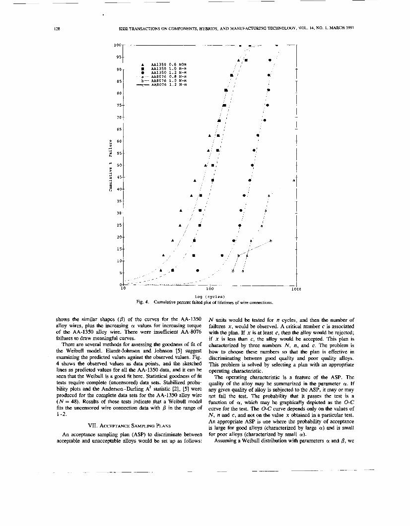
Fig. 4 shows the same data using the cumulative probability scale, and showing the fitted probability distributions for AA- 1350 alloy wires, using ML estimators for (Y and @. This graph

127

) O

TABLE I SUMMARY OF WIRE TESTS. NUMBER OF SAMPLES FAILED AT VARIOUS

ESTIMATES OF WEIBULL PARAMETERS CY, 0 NUMBER OF CYCLES, PLUS 95% CONFIDENCE INTERVALS FOR

Torque N failed (of 16) Weibull Parameter Estimates Alloy (N-m) (at cycles) + 95 % Confidence Intervals

500 700 lo00 (6 ai a;) (j p̂ $1

1350 0.8 16 16 16 85 116 156 1.2 1.7 2.5 1.0 16 16 16 111 143 185 1.4 2.0 2.9 1.2 15 16 16 305 373 456 1.7 2.5 3.8

8076 0.8 6 6 7 713 1372 2638 0.7 1.3 2.5 1.0 2 3 3 510 6619 85840 0.3 0.8 2.4 1.2 0 0 0'

' Weibull parameters could not be estimated for this condition, because no failures occurred.

128 IEEE TRANSACTIONS ON COMPONENTS, HYBRIDS, AND MANUFACTURING TECHNOLOGY, VOL. 14, NO. 1 , MARCH 1991

95-

90.-

8 5 %

80--

7 5--

70-

6 5.-

60.- 7 4 rl

4 55-

* SO-- > 2 4 5 5 a

40-

35-

30--

25--

20--

15.-

10.-

5.-

A AA1350 0 . 8 NOm W AA1350 1 . 0 N-MI

AA1350 1 . 2 N-m

-b- AA8016 1 . 0 N-m =c= AA0076 1 . 2 N-m

m - a - AA8076 0 . 8 N-m

m l I

I I

- 1 I !

I , ' I

I

A W '

I !

A .I I

I

A ,'. 0

I

e, ,

&

' e

e,'

.'

? a

A e' P b , ' ,' $

i i- A .

/

' 1 / '

d d

_ - _ _ - - - _ - 0 - - 10 100 1

log (cycles) Fig. 4. Cumulative percent failed plot of lifetimes of wire connections.

shows the similar shapes ((3) of the curves for the AA-1350 alloy wires, plus the increasing a values for increasing torque of the AA-1350 alloy wire. There were insufficient AA-8076 failures to draw meaningful curves.

There are several methods for assessing the goodness of fit of the Weibull model. Elandt-Johnson and Johnson IS] suggest examining the predicted values against the observed values. Fig. 4 shows the observed values as data points, and the sketched lines as predicted values for all the AA-1350 data, and it can be seen that the Weibull is a good fit here. Statistical goodness of fit tests require complete (uncensored) data sets. Stabilized proba- bility plots and the Anderson-Darling A' statistic [2], [51 were produced for the complete data sets for the AA-1350 alloy wire (N = 48). Results of these tests indicate ,that a Weibull model fits the uncensored wire connection data with /3 in the range of 1-2.

VII. ACCEPTANCE SAMPLING PLANS An acceptance sampling plan (ASP) to discriminate between

acceptable and unacceptable alloys would be set up as follows:

N units would be tested for n cycles, and then the number of failures x , would be observed. A critical number c is associated with the plan. If x is at least c, then the alloy would be rejected; if x is less than c, the alloy would be accepted. This plan is characterized by three numbers N, n, and c. The problem is how to choose these numbers so that the plan is effective in discriminating between good quality and poor quality alloys. This problem is solved by selecting a plan with an appropriate operating characteristic.

The operating characteristic is a feature of the ASP. The quality of the alloy may be summarized in the parameter a. If any given quality of alloy is subjected to the ASP, it may or may not fail the test. The probability that it passes the test is a function of a, which may be graphically depicted as the 0-C curve for the test. The 0-C curve depends only on the values of N, n and c, and not on the value x obtained in a particular test. An appropriate ASP is one where the probability of acceptance is large for good alloys (characterized by large a) and is small for poor alloys (characterized by small a).

Assuming a Weibull distribution with parameters a and (3, we

. .

JOYCE: MODEL TO CHARACTERIZE LIFETIMES OF ELECTRICAL WIRE CONNECTIONS 129

1.0

0.6

10 o.21 0.0 4 IO0 1500

- 6 - 2 9 A 3000

oc of& OC

Fig. 5. Operating characteristic curves for Weibull distribution with 0 = 2. Accept group if less than c failures in N samples. Curves show probabilities of acceutance where Drobabilitv of (discriminating between a = 400, 1500)

I \

> 0.9,

may calculate the probability of observing x failures out of a set of N samples tested, as follows.

Probability of (exactly x failures in N tested):

= ( :) prob ( x failures) prob ([ N - x ] continuing)

= ( y ) prob (1 failure) * prob (1

(4)

We may then calculate the probability of observing at least c failures in a set of N samples, by summing the individual probabilities calculated from (4), for various numbers of cycles completed. The probability of observing at least c failures in N samples, is the sum of observing exactly c failures + exactly (c + 1) failures, and so on, up to exactly N failures. These probabilities were calculated for various combinations of N samples, n cycles, and for values of 6 ranging from 1 to 2.

Fig. 5 shows 0-C curves for discriminating between items

with a = 400 and a = 1500 (highest 6 for AA-1350 versus lowest 6 for AA-8076, from tests reported here), assuming a Weibull distribution with 6 = 2. The 0-C curves with the best ability to discriminate, are those with an almost vertical slope, that is with a low probability of failing the test if the material has a high characteristic lifetime (a), and a high probability of failing the test if the material has a low characteristic lifetime (a).

Fig. 5 contains only the 0-C curves for N = 10, 20, 30, and n = 300, 500, 1O00, for which the probability of accepting an alloy with a < 400 is less then 0.05, and the probability of rejecting an alloy with a > 1500 is less than 0.05.3 It can be seen that a low values of N and n, there are not very many acceptance plans that discriminate between alloys with the two values of a. At high values of N and n, there are many plans to

~n fact, for N = 10, to 300 cycles, there are no acceptance plans with probability (making wrong decision) < 0.05. The closest plan has c = 2 (reject if there are at least c failures in 10 samples, to 300 cycles); with this plan, probability (rejecting alloy, if a < 400) = 0.031, and probability (rejecting alloy, if a > 1500) = 0.056.

.. .

130 IEEE TRANSACTIONS ON COMPONENTS, HYBRIDS, AND MANUFACTURING TECHNOLOGY, VOL. 14, NO. 1 , MARCH 1991

TABLE II EXAMPLES OF EFFICIENT ACCEPTANCE PLANS, ROBUST TO @ IN (1,2),

TO DISCRIMINATE BETWEEN Low AND HIGH VALUES OF a. PLANS REQUIRING MINIMUM SAMPLES AND/OR CYCLES, FROM ALL

PLANS USING 10-30 SAMPLES, RUNNING 100-loo0 CYCLES

a a N c ncycles N c ncycles low high smallest N shortest time

200 lo00 10 7 600 16 7 200 200 1500 10 5 300 12 5 200 400 1500 14 11 lo00 22 10 400 500 2000 14 9 900 27 9 400

Acceptance Plan: Test N samples to ncycles cycles; observe x , number of failures. If x < c, then accept; else, reject.

TABLE III ACCEPTANCE PLANS, WEIBULL DISTRIBU~ON FOR @ = 1-2;

PROBABILITY (ACCEPT ALLOY WITH a > 1500, REJECT

FAILURES IN N SAMPLES, RUNNING n CYCLES. ORDERED BY NUMBER OF CYCLES.

IF a < 400 CYCLES) > 0.95; REJECT IF AT LEAST c

400 400 400 400 400 400 400 400 400 500 500 500 500 500 500 500 500 500 500 500 500 600 600 600 600 600 600 600 600 600 600 600 6(K)

22 10 23 10 24 11 25 11 26 12 27 12 28 12 29 13 30 13 19 10 20 10 21 11 22 11 23 12 24 12 25 13 26 13 27 14 28 14 29 15 30 15 17 10 18 11 19 11 20 12 21 12 22 13 23 13 24 14 25 15 26 15 27 16 28 16

600 600 700 700 700 700 700 700 700 700 700 700 700 700 700 700 700 800 800 800 800 800 800 800 800 800 800 800 800 800 800 800 900

n n n cycles N c cycles N c cycles N c

29 17 900 16 12 30 17 900 17 13 16 10 900 18 13 17 11 900 19 14 18 12 900 20 15 19 12 900 21 15 20 13 900 22 16 21 13 900 23 17 22 14 900 24 17 23 15 900 25 18 24 15 900 26 19 25 16 900 27 20 26 17 900 28 20 27 17 900 29 21 28 18 29 18 30 19 16 11 17 12 18 12 19 13 20 14 21 14 22 15 23 16 24 16 25 17 26 18 27 18 28 19 29 20 30 20

900 lo00 lo00 lo00 lo00 lo00 lo00 lo00 lo00 lo00 lo00 lo00 lo00 lo00 lo00 lo00 lo00 lo00

30 22 14 11 15 12 16 12 17 13 18 14 19 15 20 15 21 16 22 17 23 18 24 18 25 19 26 20 27 21 28 21 29 22 30 23

15 I1

choose from, each very good at discriminating between the

Because there are many plans to choose from, we may generate several plans for various values for /3, and then select plans which are valid for a range of /3 values. These plans would be robust to the value of &-that is, for a /3 within a range of values, the probability of rejecting an alloy with a > 1500 is less then 0.05, and the probability of accepting an alloy with a < 400 is less than 0.05.

alloys.

TABLE N ACCEPTANCE PLANS, WEIBULL DISTRIBUTTON FOR p = 1-2; PROBABILITY (ACCEPT ALLOY WITH (Y > 1500, REJECT IF

FAILURES IN N SAMPLES, RUNNING n CYCLES. ORDERED BY N SAMPLES TESTED

(Y < 400 CYCLES) > 0.95; REIECT IF AT LEAST c

n n n cycles

lo00 900

lo00 700 800 900

lo00 600 700 800 900

lo00 600 700 800 900

lo00 500 600 700 800 900

lo00 500 600 700 800 900

lo00 500 600 700 800

N c ~~

14 11 15 11 15 12 16 10 16 11 16 12 16 12 17 10 17 11 17 12 17 13 17 13 18 11 18 12 18 12 18 13 18 14 19 10 19 11 19 12 19 13 19 14 19 15 20 10 20 12 20 13 20 14 20 15 20 15 21 11 21 12 21 13 21 14

cycles

900 lo00 400 500 600 700 800 900

lo00 400 500 600 700 800 900

lo00 400 500 600 700 800 900

lo00 400 500 600 700 800 900

lo00 400 500 600

N c

21 15 21 16 22 10 22 11 22 13 22 14 22 15 22 16 22 17 23 10 23 12 23 13 23 15 23 16 23 17 23 18 24 11 24 12 24 14 24 15 24 16 24 17 24 18 25 11 25 13 25 15 25 16 25 17 25 18 25 19 26 12 26 13 26 15

cycles

700 800

9 0 0 1000 400 500 600 700 800 900

1000 400 500 600 700 800 900

1000 400 500 600 700 800 900

1000 400 500 600 700 800 900

1000

N c

26 17 26 18 26 19 26 20 27 12 27 14 27 16 27 17 27 18 27 20 27 21 28 12 28 14 28 16 28 18 28 19 28 20 28 21 29 13 29 15 29 17 29 18 29 20 29 21 29 22 30 13 30 15 30 17 30 19 30 20 30 20 30 23

VIII. DISCRIMINATION BETWEEN ALUMINUM ALLOYS FOR WIRE CONNECTIONS

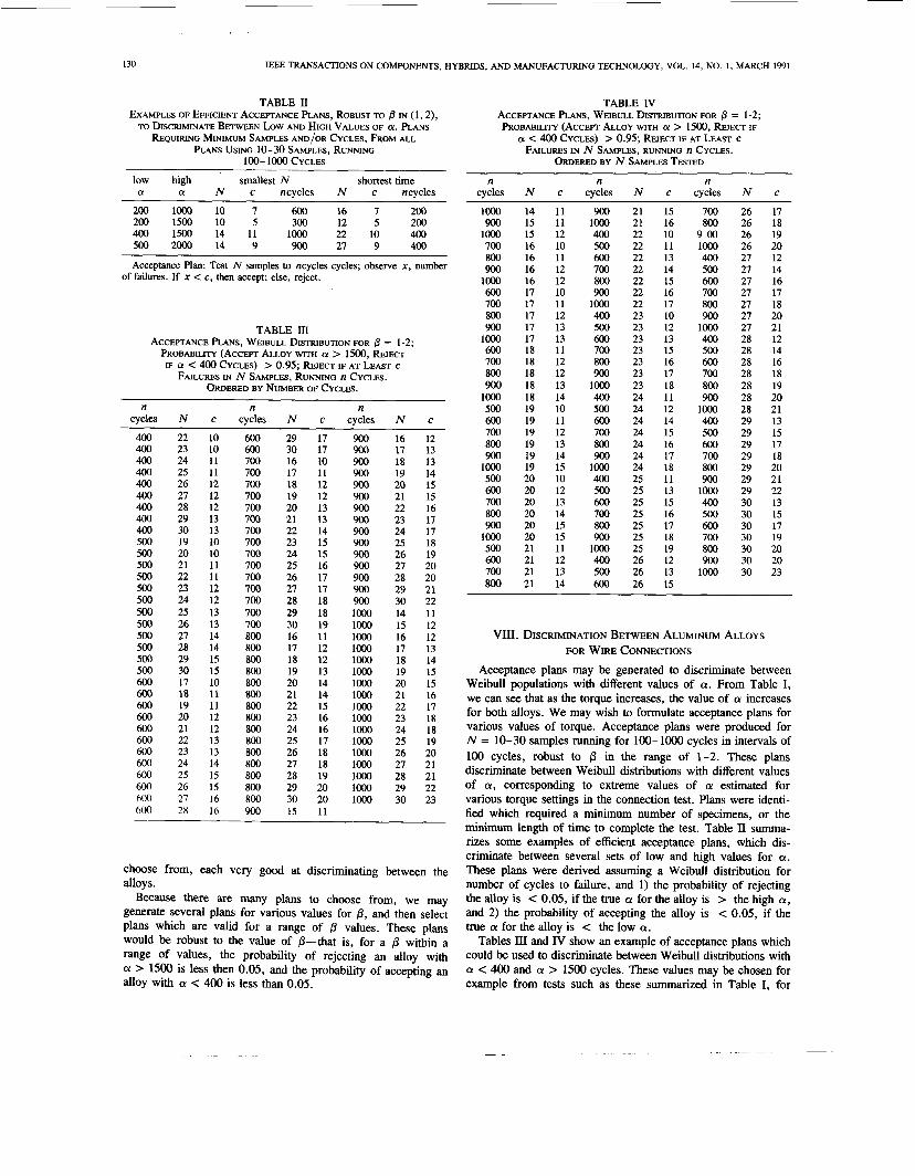
Acceptance plans may be generated to discriminate between Weibull populations with different values of a. From Table I, we can see that as the torque increases, the value of a increases for both alloys. We may wish to formulate acceptance plans for various values of torque. Acceptance plans were produced for N = 10-30 samples running for 100- loo0 cycles in intervals of 100 cycles, robust to /3 in the range of 1-2. These plans discriminate between Weibull distributions with different values of a, corresponding to extreme values of a estimated for various torque settings in the connection test. Plans were identi- fied which required a minimum number of specimens, or the minimum length of time to complete the test. Table II summa- rizes some examples of efficient acceptance plans, which dis- criminate between several sets of low and high values for a. These plans were derived assuming a Weibull distribution for number of cycles to failure, and 1) the probability of rejecting the alloy is < 0.05, if the true a for the alloy is > the high a, and 2) the probability of accepting the alloy is < 0.05, if the true a for the alloy is < the low a.

Tables III and IV show an example of acceptance plans which could be used to discriminate between Weibull distributions with a < 400 and a > 1500 cycles. These values may be chosen for example from tests such as these summarized in Table I, for

.I ,

JOYCE: MODEL TO CHARACTEFUZE LIFETIMES OF ELECTFUCAL WIRE CONNECTIONS 131

TABLE V SUMMARY OF TESTS, NUMBER OF FAILURES AT DIFFERENT NUMBER

OF CYCLES, PLUS VERDICT AFTER APPLYING ACCEPTANCE PLAN FROM TABLE III. (ALL TESTS HAD

N = 16 SAMPLES TESTED)

n c,min# n wire Torque failed failures

Test cycles Alloy (N-m) (/16) = reject verdict 16 fail 16 fail 16 fail

6 pass 3 pass 0 pass

1350 0.8 1350 1.0 1350 1.2

8076 0.8 8076 1.0 8076 1.2

700 11

A 1350 0.8 16 fail 1350 1.0 16 fail 1350 1.2 16 fail

lo00 13 8076 0.8 7 pass 8076 1.0 3 pass 8076 1.2 0 pass

1350 1.0 16 fail 1350 1.2 14 fail

8076 1.0 5 pass 8076 1.2 0 pass

700 11

B 1350 1.0 16 fail 1350 1.2 16 fail

8076 1.0 6 pass 8076 1.2 0 pass

lo00 13

wire connections with 1 .O-N-m torque. The acceptance plan was produced for N = 10-30 samples, running for 100-lo00 cy- cles, and these are shown in Table III and IV. For all these combinations of N, c, and n cycles, if the true CY is < 400 cycles, 95% of the time we will observe at least c failures in N samples tested to n cycles; similarly, if the true a is > 1500 cycles, 95% of the time we will observe less than c failures in N samples tested to n cycles.

E. SPECIFICATION OF A TEST TO DISCRIMINATE BETWEEN AL ALLOYS FOR WIRE CONNECTIONS

Based on this analysis of lifetimes of aluminum electrical wire connections, assuming a Weibull distribution with P ranging from 1 to 2, and a characteristic life for AA-8076 alloy of at least 1500 cycles, and for AA-1350 of at most 400 cycles, then Tables 111 and IV may be used to select conditions to run a test to discriminate between the alloys.

Using Table III, a test may be chosen on the basis of the desired number of cycles, or a test in progress may be monitored by checking the critical values for failure at intervals during the test period. Using Table IV, a test may be chosen on the basis of number of samples available to be tested, or if a test in progress loses test items for some reason other than failure, an alternative acceptance plan may be used, without stopping the test. It can be seen that the minimum number of samples to distinguish be- tween the alloys is 14 (running to lo00 cycles), and the mini- mum number of cycles is 400 (using 22 samples).

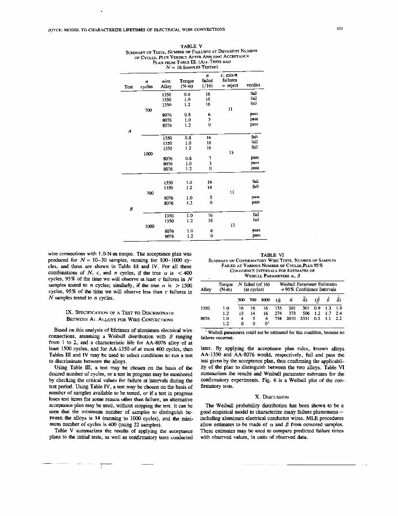
Table V summarizes the results of applying the acceptance plans to the initial tests, as well as confirmatory tests conducted

TABLE VI SUMMARY OF CONFIRMATORY WIRE TESTS. NUMBER OF SAMPLES

FAILED AT VARIOUS NUMBER OF CYCLES,PLUS 95% CONFIDENCE INTERVALS FOR ESTIMATES OF

WEIBULL PARAMETERS (Y, 0 Torque N failed (of 16) Weibull Parameter Estimates

Alloy (N-m) (at cycles) + 95 % Confidence Intervals

500 700 lo00 (4 oi 8) (h p^ j) 1350 1.0 16 16 16 135 201 301 0.9 1.3 1.9

1.2 13 14 16 274 373 506 1.2 1.7 2.4 8076 1.0 4 5 6 758 2010 5331 0.5 1.1 2.2

1.2 0 0 0'

' Weibull parameters could not be estimated for this condition, because no failures occurred.

later. By applying the acceptance plan rules, known alloys AA-1350 and AA-8076 would, respectively, fail and pass the test given by the acceptance plan, thus confirming the applicabil- ity of the plan to distinguish between the two alloys. Table VI summarizes the results and Weibull parameter estimates for the confirmatory experiments. Fig. 6 is a Weibull plot of the con- firmatory tests.

X. DISCUSSION The Weibull probability distribution has been shown to be a

good empirical model to characterize many failure phenomena- including aluminum electrical conductor wires. MLE procedures allow estimates to be made of a and from censored samples. These estimates may be used to compare predicted failure times with observed values, in units of observed data.

132 IEEE TRANSACTIONS ON COMPONENTS, HYBRIDS, AND MANUFACTURING TECHNOLOGY, VOL. 14, NO. 1, MARCH 1991

0.999

0.99

0.95

0.9

0 . 8

0 . 6 3

0.s

>t 5 0.3 4 ..I P m

% 0.2 P

al

U a 0 . 1

0.05

0.0;

0 . 0 1

0.001

- -t - AA1350 1.0 N-m - a.- AA1350 1.2 N-m -b- AA8076 1.0 N-m =C=AA8076 1.2 N-m

100

log (cycles)

Fig. 6. Weibull plot of the lifetimes of wire connections, confirmatory tests.

Characterization of lifetimes of electrical connections has been done previously using the Arrhenius method, as summarized in the 1986 CAE report [20]. Using this method, the test is continued until 50% of the samples have failed, and then the cycle number is recorded, as well as the steady-state temperature for the first ON portion of the test. Repeated runs of sets of samples are required, to obtain data points (l/Temperature versus cycle time for 50% of samples) for plotting on the Arrhenius scale, and hence, many samples tested (10) yield only one data point for plotting.

The Weibull model and ML methods that estimate parameters, uses d l of the data observed (cycle number to failure or still- continuing), and requires fewer samples than the Arrhenius method, and hence, is proposed as a more suitable method to characterize lifetimes of electrical connections. From the analy- sis done here, the Weibull model also fits the observed data very well.

Assuming a Weibull model to quantify characteristics of aluminum electrical wire connections, it may be of interest to

J 1000

determine if the /3 is a constant, characteristic of aluminum wire, and also to estimate it. The test done here with the complete data sets for AA-1350 wire indicate that /3 may be a constant for these test types, and in the range of 1-2. Tests run to 100% failure would be prohibitively long.4 However, for the purposes of discriminating between two alloys with quite differ- ent CY, the procedure as outlined here may be used to develop acceptance plans which are robust to a range of values for P.

ACKNOWLEDGMENTS Thanks to Paul Schell of Alcan KRDC for his careful work in

setting up and running the tests, data recording, and comments and feedback on using the Weibull MLE computer programs, and also to Gord Murphy of Alcan KRDC who helped make the programs run more efficiently. Thanks to Alcan Wire and Cable, Toronto, and Stephen Keeley of KRDC who, respectively,

Complete failure of the AA-8076 connections, to (estimated) 10 000 cycles, would require more than a year!

JOYCE: MODEL TO CHARACTERIZE LIFETIMES OF ELECTRICAL WIRE CONNECTIONS 133

sponsored and directed the testing, and to Bob Edwards of Alcan Wire and Cable for his guidance. Much appreciation to Louis Broekhoven of Queen’s University, who supervised this project for an M.Sc. degree at Queen’s.

r31

r41

r51

161

[71

[81

[91

REFERENCES

T. Allen, Particle Size Measurement, 3rd Ed. London, U.K.: Chapman and Hall, 1981. L. Broekhoven and R. Jahan, “Testing for the exponential distri- bution with large numbers of s m a l l samples,” Queen’s Univ. Dep. Math. Statistics Preprint 1987-13, 1987. M. Calvo, “Application of the Weibull statistics to the characteri- zation of metallic glass ribbons,” J. Mat. Sci., vol 24, no. 5 , 1989. “Nonmetallic Sheathed Cable: Wiring Products,” CSA Standard C22.2 No. 48-M1984, Canadian Standards Association, Toronto, 1984. R. C. Elandt-Johnson and N. L. Johnson, Survival Models and Data Analysis. Toronto, Canada: Wiley, 1980. A. J. Gross and V. A. Clark, Survival Distributions: Reliabil- ity Applications in the Biomedical Sciences. Toronto, Canada: Wiley, 1975. G. J. Hahn and S . S . Shapiro, Statistical Models in Engineer- ing. Toronto, Canada: Wiley, 1967. C. C. Harris, “The application of size distribution equations to multi-event cornmunition processes,” Trans. AIMEISME, vol.

- , “Graphical presentation of size distribution data: An as- sessment of current practice,” Trans. IMM (C), vol. 80, pp.

241, pp. 343-358, 1968.

C133-CI39. 1971.

r131

1141

[151

1161

1201

“Fatigue of ceramics (Part 2)-Cyclic fatigue properties of sin- tered Si,N, at room temperature,” J. Cer. Soc. Japan, vol. 97, no. 5 , 1989. Y. Matsuo, T. Oida, K. Jinbo, K. Yasuda, and S. Kimura, “Analysis of fatigue life of ceramics using multi-modal Weibull distribution,” J . Cer. Soc. Japan, vol. 97, no. 2, 1989. J. Natesan and A. K. S . Jardine, “Graphical estimation of mixed Weibull parameters for ungrouped multicensored data: Its appli- cation to failure data,” Maint. Manag. Znt., vol. 6, pp.

W. Nelson, Applied Life Data Analysis. Toronto, Canada: Wiley, 1982. - , “ASQC basic references in quality control: Statistical tech- niques, Volume 6: How to analyse reliability data,” Amer. Soc. for Quality Control, 1983. R. R. Rider, “Estimating the parameters of mixed Poisson, bionomial, and Weibull distributions by the method of moments,”

P. Rosin and E. Rammler, “The laws governing the fineness of powdered coal,” J. Inst. Fuel, vol. 7, pp. 29-36 and 109-112, 1933. Y. Sasaki, A. Kuichi, T. Shinke, T. Minato, T. Nishi, and K. Sugii, “Fatigue resistance analysis of corroded wire,” Kobefco Technol. Rev., no. 4. Aug. 1988. K. J. Smith and R. S . Timsit, “Electrical connectability of aluminum wire,” Rep. Canadian Electrical Association, CEA No. 76-19, Part B, 1985. F. H. Steiger, “Practical applications of the Weibull distribution function,” Chem. Tech., pp. 225-231, Apr. 1971. M. Sutcu, “Weibull statistics applied to fiber failure in ceramic composites and work of fracture,” Acta Metall., vol. 37, no. 2,

115-127, 1986.

ISI Bull. vol. 39, part 2, pp. 225-232, 1962.

[lo] 1989. Rep. on NEMA Research Project Aluminum Terminations, AP- pendix A, Underwriters’ Laboratories, May 11, 1981.

[111 J. H. K. Estimation of Mixed Weibull [24] W. Weibull, “A statistical theory of the strength of materials,” Ing. VelenskapsAkad. Handl. vol 151 pp. 1-45, 1939. distriiutio; ful;ction of wide applica- bility,” J. Appl. Mech., Sept. 1951.

H. E. Hill, “Application of the Weibull Distribution Function in the Coatings Industry,” journal of Coatings Technology, vol. 48, no. 619, August 1976.

Parameters in Life-Testing of Electron Tubes,” Technometrics, vol 1, no. 4, 1959, pp. 389-407. M. Masuda, N. Yamada, T. Soma, M. Matsui, and I. Oda,

[23I

[251 W. Weibull, ,,A [12]