A Weather Disaster Management - Suny...

A Weather Disaster Management (Baton Rouge, LA & Hurricane Sandy)

Group 5: Qingpei REN Xin LI Yapan LIU Yigang QIAN Ziyu MA

Reference: https://en.wikipedia.org/wiki/Hurricane_Sandy

Reference: https://www.google.com/maps/place/Baton+Rouge,+LA/@30.4968783,-91.5069376,9.82z/data=!4m5!3m4!1s0x86243867325f74cb:0x2123f1db91579a1d!8m2!3d30.4582829!4d-91.1403196

Reference: https://www.google.com/search?q=sandy+storm+baton+rouge+2012&newwindow=1&source=lnms&tbm=isch&sa=X&ved=0ahUKEwjf86mTmZHSAhVHNSYKHUZaA1EQ_AUICigD&biw=1536&bih=735

Before(long time

period)

Before(short

time/after being

monitored)

-ing Emergency

response

After

Government

Storage shelter

Reinforce building

Picking the safety

place

Storage food

Storage boat(large

and small)

Storage barrier staff

River management

(Mississippi)

Emergency(medical

workers, fireman,

policeman, guard)

Education(facing

disaster, manoeuver)

Experiment

Evacuate

people(using car,

helicopter, boat)

River management

(drain away water)

Emergency(medical

workers, fireman,

policeman, guard)

Reinforce house

Food and other

staffs’ transportation

News report (inform

public)

Evaluate the disaster

Maintain electronic

and communication

running smoothly

River management

(drain away water)

Distribute food and

stuff

Emergency(medical

workers, fireman,

policeman, guard)

Rescue

Transport the

refugee and rescuer


Allocation

Red cross and the

other organization

(donation)

News report (inform

public)

Maintain electronic

and communication

running smoothly

River management

(drain away water)

Distribute food and

stuff

Rebuild house

Inform people back

to their home

News report

Physical and mental

help


Red cross and the

other organization

(donation)

News report (inform

public)

Insurance

Experiment

Monitoring hurricanes

Disaster resp onse training

Reserve basi c living suppl ies

Reinforced h ouses

Set flood pre vention obst acles

Clean street hazards

Build shelter s at high altit ude

Safe depart ment keep s afety

Transfer resi dents to shel ters Rescue victi

ms

Identify iden tity

Send to shel ter and recei ve basic livi ng stuffs

Send to hos pital and rec eive treatme nt

Infection dis eases preven tion and con trol

Collection of deceased rel ics

Treatment of corpses

A

A

Basic living fa cilities reconst ruction

Houses recons truction

Transport resi dents

Return collectio ns of victims to their families

Record data an d analyze

Prepare for t he next disas ter

No

Detected Yes

No

Yes Alive

Yes

Injured No

Beginning

End

Cost of Poor Quality

Process Internal Failure External Failure Appraisal Prevention

Monitoring the hurricane Equipment Failure

Technique Support

Reinforce Houses Lack Building Technique Training

Disaster Response Training Absence

The strength level

Periodic Education

Food Storage Storage equipment broken Theft Food storage

policy Periodic Check

Evacuation of People Time and WF shortage

Reluctant to evacuate How & Where

Search and Rescue

Time and WF shortage/Road blockage

Clear road blockage

Injury Judgment Wrong judgment The level of

injury Training

Provide Basic Living Needs

Expired food, shelter collapse Examination

Treatment of the Injured WF & Equipment shortage

Scramble for goods

Basic living standard

Transportation of Injuries Vehicle damage Examination

Disease Control

Drinking water polluted/Corps not well

dealt Refuse to follow

the rules Make

regulations

Rebuild Building Material/Techiques Surfering disater Strength of the

building

ase the cost)

Quality(Incre

Poor

Organizations

Media

Residents

Emergency

Rescue Department

Government

barrier

Poor quality of the

Failure

River management

monitoring system

Low accuracy of

Poor shelters’ quality

medicine

Not enough food and

failure

Medicine and storage

Insufficient equipments

Insufficient staff

Low efficiency staff

system failure

Communication

system failure

Power transmission

staff

Insufficient trained

technology

Out of dated

of the disaster

Insufficient awareness

knowledge

Insufficient self rescue

accuracy

efficiency and

Low forecast

Late news update

Insufficient funds

volunteers

Insufficient trained

Root - Cause Diagram

Six Sigma

Define

Measure

Analyze Improve

Control

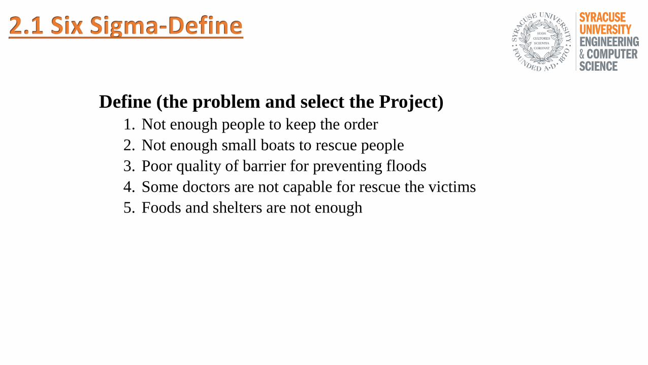
Define (the problem and select the Project)

1. Not enough people to keep the order

2. Not enough small boats to rescue people

3. Poor quality of barrier for preventing floods

4. Some doctors are not capable for rescue the victims

5. Foods and shelters are not enough

Measure (identified Quality parameters using

specific methods)

• Verify the project needs

• Document the process

• List of possible X’s that impact Y

• Plan for data collection

Questions X Did not solve Y

Shortage of people keep order Looting, fighting, people get hurt even

killed, chaos.

Shortage of small boats to rescue

victims

Cannot transferred and rescue the

victims in time.

Poor quality barriers Cannot stop the flood, resulting in

water level increased and led to

secondary disaster.

Doctors cannot handle treatment tasks Cannot timely rescue the patient led to

life-long disability or even death.

Shortage of foods and shelters The victims do not get food and shelter,

cause robbery and fights and other

chaos incidents.

List of possible X’s that impact Y

Generate random data

Before After

101.774 101.072

100.338 101.596

101.655 100.409

100.686 99.837

99.712 100.317

100.086 100.080

98.704 100.094

98.939 102.056

99.206 99.059

99.355 98.272

101.613 101.755

100.626 100.128

101.065 101.256

98.111 99.804

98.618 100.008

100.012 99.639

100.922 100.099

100.396 99.511

99.983 100.365

99.420 100.209

Analyze(Generate random data, using

Minitab)

Data collection planning

ANOVA

AfterBefore

100.75

100.50

100.25

100.00

99.75

99.50

Data

Interval Plot of Before, After95% CI for the Mean

The pooled standard deviation is used to calculate the intervals.

AfterBefore

102

101

100

99

98

Data

Boxplot of Before, After

Improve (provide some solutions to the problem

detected)

Tools

Improvement strategy

Process FMEA

Design of experiments (DOE)

Benchmarking

Mistake proofing

Lean event

Poor quality of barrier for preventing floods

1. FMEA: Poor quality of barrier for preventing floods

2. DOE: Testing the performance of barrier materials

3. Improvement Strategy: According to degrees of

floods, prepare different level barrier materials

Example:

Control (the solutions and ensure their permanent

implementation)

Tools-5S

Sort

Set in order

Shine

Standardize

Sustain

For the problem of “Some doctors are not capable

for rescuing the victims” 1. Sort: Classify the doctors concentrating in different area

for emergency calling.

2. Set in order: Flow Chart of doctors for dealing with

emergency processes.

3. Shine: Put the criteria on the Remarkable Places

4. Standardize: Make check list to see whether all the

equipment and people are working well

5. Sustain: Rating system keep everyone understanding the

process

Example:

DOE (Design of experiments)

Row Time Temp Catalyst Yield

1 50 200 A 48.4665

2 20 200 A 45.1931

3 50 200 B 49.204

4 50 150 B 45.5991

5 20 150 A 42.7636

6 50 150 A 44.7592

7 20 200 B 44.7077

8 20 150 B 43.3937

9 50 200 A 49.0645

10 50 150 B 45.1531

11 50 200 B 48.672

12 20 200 B 45.3297

13 50 150 A 45.3932

14 20 150 B 43.0617

15 20 150 A 43.2976

16 20 200 A 44.8891

Objective: Perform a Complete DOE 2^3 Full Factorial design with the data above (notice, TWO replications per treatment) using, both of these methods and verify your similar results. 1. an Excel Spread Sheet 2. Minitab Regression model

Factor Low Level (-1) High Level (+1)

Time 20 50

Temp 150 200

Catalyst A B

Excel Spread Sheet (Full Factorial Design) Coding

A-Time B-Temp C-Catalyst AB AC BC ABC Y1 Y2

1 1 1 1 1 1 1 1 48.4665 49.0645 48.7655

2 -1 1 1 -1 -1 1 -1 45.1931 44.8891 45.0411

3 1 1 -1 1 -1 -1 -1 49.204 48.672 48.938

4 1 -1 -1 -1 -1 1 1 45.5991 45.1531 45.3761

5 -1 -1 1 1 -1 -1 1 42.7636 43.2976 43.0306

6 1 -1 1 -1 1 -1 -1 44.7592 45.3932 45.0762

7 -1 1 -1 -1 1 -1 1 44.7077 45.3297 45.0187

8 -1 -1 -1 1 1 1 -1 43.3937 43.0617 43.2277

Avg. @-1 44.07953 44.17765 45.64013 45.12803 45.59645 45.51588 45.57075

Avg. @1 47.03895 46.94083 45.47835 45.99045 45.52203 45.6026 45.54773

Effect 2.959425 2.763175 -0.16177 0.862425 -0.07442 0.086725 -0.02302

Estimate 1.479713 1.381588 -0.08089 0.431213 -0.03721 0.043363 -0.01151

Var @-1 0.109335 0.124532 0.122381 0.135022 0.107439 0.169628 0.110953

Var @1 0.155188 0.139991 0.142142 0.129501 0.157084 0.094895 0.15357

F 1.419376 1.124141 1.161467 0.959114 1.462072 0.559432 1.384106

RegCoef b1 b2 b3 ab b0

Estimat. 1.479713 1.381588 -0.08089 0.431213 45.55924

Regression Estimations

Run

Factors and Interactions Replicated response values

Avg.

Var. of Model 0.132261 StdDv 0.363677

Var. of Effect 0.033065 StdDv 0.181839

Degree of Freedom 16

Student T (0.025;DF) 2.472878

C.I. Half Width 0.449665

Factor A B C AB AC BC ABC

Significant? Yes Yes No Yes No No No

Criteria: Absolute value of Effect > C.I. Half Width

Excel DOE

Minitab DOE

A-Time B-Temp C-Catalyst Y StdOrder RunOrder Blocks CenterPt

1 1 1 48.4665 1 1 1 1

-1 1 1 45.1931 2 2 1 1

1 1 -1 49.204 3 3 1 1

1 -1 -1 45.5991 4 4 1 1

-1 -1 1 42.7636 5 5 1 1

1 -1 1 44.7592 6 6 1 1

-1 1 -1 44.7077 7 7 1 1

-1 -1 -1 43.3937 8 8 1 1

1 1 1 49.0645 9 9 1 1

-1 1 1 44.8891 10 10 1 1

1 1 -1 48.672 11 11 1 1

1 -1 -1 45.1531 12 12 1 1

-1 -1 1 43.2976 13 13 1 1

1 -1 1 45.3932 14 14 1 1

-1 1 -1 45.3297 15 15 1 1

-1 -1 -1 43.0617 16 16 1 1

QFD and VSM (Quality Function Deployment)

QFD-- How it works？ 1.Quality Function Deployment methodology involves several sequential

phases. 2.During each phase one or more matrices are prepared. 3.Matrices help to plan and communicate critical product and process

planning and design information.

Trade-off

Correlation

Competition

Targets How much

Voice of Customer

Voice of Engineers

Value Stream Map (As a tool to Implement Lean Event)

1.Lean Event: More value with less work. 2.Lean Tools: VSM; 5S; Kanban; Takt Time… 3.Lean & 3 evil M’s: MUDA--Waste activities; MURA-- Inconsistent Use of

people; MURI-- Excessive demands on people/ processes. 4.Define VSM: The process for stored food to be disseminated.

Current VSM Future VSM

Implementation Plan in Steps

1. Hold training to clarify the concept of Lean process;

2. Constitute Group for collecting data for each process and to Analysis collected dat;

MSA (Measurement System Analysis)

Gage R&R Information Session We have three inspectors to detect the water level of the river, each of them detect the water level three times at the same time (8:00 AM, 16:00 PM, 00:00 AM), and compare them with the standard value. With these data, the Weather Forecast Office can decide to give Flood Warning or not. We choose some data from ten days and analyze this set of data, to find out if there are some factors can affect the results. We use a standard value of water level---25 feet.

Major Flood Stage: 40

Moderate Flood Stage: 38

Flood Stage: 35

Action Stage: 30

Flood Categories (in feet)

Day Monitor Measurement Monitor Measurement Monitor Measurement

1 A 2.9 B 0.8 C 0.4

1 A 4.1 B 2.5 C -1.1

1 A 6.4 B 0.7 C -1.5

2 A -5.6 B -4.7 C -13.8

2 A -6.8 B -12.2 C -11.3

2 A -5.8 B -6.8 C -9.6

3 A 13.4 B 11.9 C 8.8

3 A 11.7 B 9.4 C 10.9

3 A 12.7 B 13.4 C 6.7

4 A 4.7 B 0.1 C 1.4

4 A 5 B 10.3 C 2

4 A 6.4 B 2 C 1.1

5 A -8 B -5.6 C -14.6

5 A -9.2 B -12 C -10.7

5 A -8.4 B -12.8 C -14.5

6 A 0.2 B -2 C -2.9

6 A -1.1 B 2.2 C -6.7

6 A -2.1 B 0.6 C -4.9

7 A 5.9 B 4.7 C 0.2

7 A 7.5 B 5.5 C 0.1

7 A 6.6 B 8.3 C 2.1

8 A -3.1 B -6.3 C -4.6

8 A -2 B 0.8 C -5.6

8 A -1.7 B -3.4 C -4.9

9 A 22.6 B 18 C 17.7

9 A 19.9 B 21.2 C 14.5

9 A 20.1 B 21.9 C 18.7

10 A -13.6 B -16.8 C -14.9

10 A -12.5 B -16.2 C -17.7

10 A -13.1 B -15 C -21.6

DATA (In feet)

We can conclude that the factors of “Day” and “Inspector” can affect the results, there is no interaction between “Day” and “Inspectors”.

Gage R&R Study - ANOVA Method Two-Way ANOVA Table With Interaction Source DF SS MS F P Day 9 8836.19 981.799 492.291 0.000 Monitor 2 316.73 158.363 79.406 0.000 Day * Monitor 18 35.90 1.994 0.434 0.974 Repeatability 60 275.89 4.598 Total 89 9464.71 α to remove interaction term = 0.05 Two-Way ANOVA Table Without Interaction Source DF SS MS F P Day 9 8836.19 981.799 245.614 0.000 Monitor 2 316.73 158.363 39.617 0.000 Repeatability 78 311.79 3.997 Total 89 9464.71

1st 2nd 1st 2nd

1 go 1 go go 2 go go

2 no 1 no no 2 no no














16 go 1 go go 2 go no

17 go 1 no no 2 no go




ResultSample Attribute inspector inspector

Result

Attribute Agreement Analysis Information Session

We have 2 people to inspect the quality of the food, to evaluate each monitor’s capability we design an Attribute Agreement Analysis. In the data set below, we have 20 samples of a same kind of food and each inspector measure them twice.

21

100

95

90

85

80

75

70

Appraiser

Perc

en

t

95.0% CI

Percent

21

100

95

90

85

80

75

70

Appraiser

Perc

en

t

95.0% CI

Percent

Date of study:

Reported by:

Name of product:

Misc:

Assessment Agreement

Within Appraisers Appraiser vs Standard

We can conclude that Inspector 1 has a better capability in “Within Appraisers” and “Appraiser vs Standard”.

Acceptance Sampling Plan (Analysis of Food Safety in Disaster Management)

Project Review

Baton Rouge after the hurricanes and floods, the supply of daily consumables is critical. Our project is doing an acceptance sampling plan to check the quality of the foods.

Binomial Nomograph

n=225 C=16

Sampling Plan Parameters Lot size = 1500

AQL = 0.05

LTPD = 0.1

α = 0.05

β = 0.1

Acceptance sampling by attributes, the

results are “Good” or “Bad”.

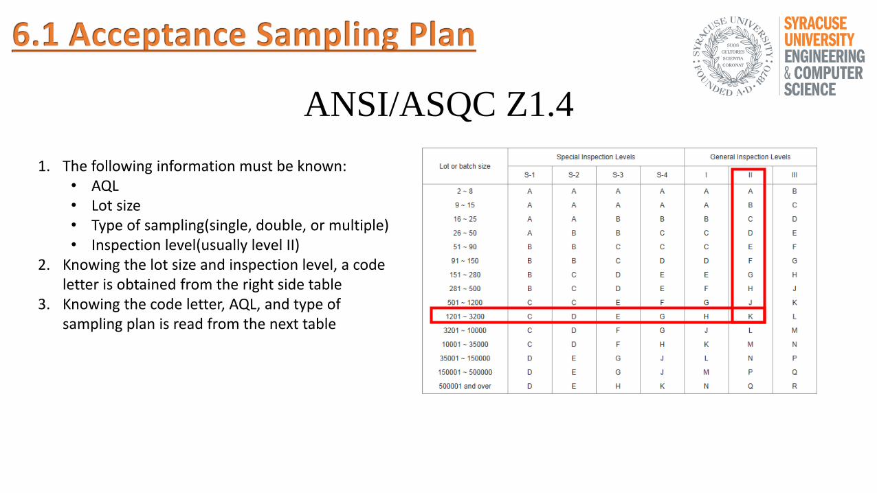
ANSI/ASQC Z1.4

1. The following information must be known: • AQL • Lot size • Type of sampling(single, double, or multiple) • Inspection level(usually level II)

2. Knowing the lot size and inspection level, a code letter is obtained from the right side table

3. Knowing the code letter, AQL, and type of sampling plan is read from the next table

Master table for normal inspection (single sampling)

n=125 c=12

Our Data

Binomial Binomial

n = 125 n = 225

c = 12 c = 16

PDPa

(Cumulative)AOQ

Average Total

Inspection

Pa

(Cumulative)AOQ

Average Total

Inspection0 1.000000 0.000000 125.0 1.000000 0.000000 225.0

0.01 1.000000 0.009167 126.0 1.000000 0.008500 226.0

0.02 0.999998 0.018333 126.0 0.999996 0.017000 226.0

0.03 0.999894 0.027497 126.0 0.999485 0.025487 226.0

0.04 0.998432 0.036609 128.0 0.990392 0.033673 238.0

0.05 0.989994 0.045375 139.0 0.939319 0.039921 303.0

0.06 0.962322 0.052928 177.0 0.803800 0.040994 476.0

0.07 0.901081 0.057819 262.0 0.591709 0.035207 746.0

0.08 0.799634 0.058640 401.0 0.367611 0.024998 1032.0

0.09 0.665182 0.054877 586.0 0.193076 0.014770 1254.0

0.1 0.516016 0.047301 791.0 0.086692 0.007369 1390.0

0.11 0.372988 0.037610 988.0 0.033740 0.003155 1457.0

0.12 0.251652 0.027682 1154.0 0.011536 0.001177 1486.0

0.13 0.158971 0.018944 1282.0 0.003506 0.000387 1496.0

0.14 0.094362 0.012110 1371.0 0.000957 0.000114 1499.0

0.15 0.052820 0.007263 1428.0 0.000237 0.000030 1500.0

0.16 0.027978 0.004103 1462.0 0.000053 0.000007 1500.0

0.17 0.014066 0.002192 1481.0 0.000011 0.000002 1500.0

0.18 0.006731 0.001111 1491.0 0.000002 0.000000 1500.0

0.19 0.003074 0.000535 1496.0 0.000000 0.000000 1500.0

0.2 0.001342 0.000246 1499.0 0.000000 0.000000 1500.0

0.21 0.000561 0.000108 1500.0 0.000000 0.000000 1500.0

0.22 0.000225 0.000045 1500.0 0.000000 0.000000 1500.0

0.23 0.000087 0.000018 1500.0 0.000000 0.000000 1500.0

0.24 0.000032 0.000007 1500.0 0.000000 0.000000 1500.0

0.25 0.000011 0.000003 1500.0 0.000000 0.000000 1500.0

OC Example OC Example

0.000000

0.100000

0.200000

0.300000

0.400000

0.500000

0.600000

0.700000

0.800000

0.900000

1.000000

0 0.05 0.1 0.15 0.2 0.25

% P

a (

Pro

bab

ility

of

Acc

epta

nce

)

% Pd ( Lot Percent Defective)

Operating Characteristic (OC) Curve

n=125, c=12

n=225, c=16

0.000000

0.010000

0.020000

0.030000

0.040000

0.050000

0.060000

0.070000

0 0.05 0.1 0.15 0.2 0.25 0.3

AO

Q (

Per

cen

t D

efec

ive)

Incoming Lot Percent Defective

Average Outgoing Quality (AOQ) Curve

n=125, c=12

n=225, c=16

0.0

200.0

400.0

600.0

800.0

1000.0

1200.0

1400.0

1600.0

0 0.05 0.1 0.15 0.2 0.25 0.3

Ave

rage

To

tal I

nsp

ecti

on


Average Total Inspection (ATI) Curve

n=125, c=12

n=225, c=16

Minitab Acceptance Sampling Acceptance Sampling by Attributes Measurement type: Number of defects Lot quality in defects per unit Lot size: 1500 Use Poisson distribution to calculate probability of acceptance Acceptable Quality Level (AQL) 0.05 Producer’s Risk (α) 0.05 Rejectable Quality Level (RQL or LTPD) 0.1 Consumer’s Risk (β) 0.1 Generated Plan(s) Sample Size 248 Acceptance Number 18 Accept lot if number of defects in 248 items ≤ 18; Otherwise reject. Defects Probability Probability Per Unit Accepting Rejecting AOQ ATI 0.05 0.951 0.049 0.03970 309.0 0.10 0.099 0.901 0.00822 1376.6 Average outgoing quality limit (AOQL) = 0.04165 at 0.05772 defects per unit.

0.000000

0.100000

0.200000

0.300000

0.400000

0.500000

0.600000

0.700000

0.800000

0.900000

1.000000

0 0.05 0.1 0.15 0.2 0.25

% P

a (

Pro

bab

ility

of

Acc

epta

nce

)


Operating Characteristic (OC) Curve

n=125, c=12

n=225, c=16

n=248, c=18

0.0

200.0

400.0

600.0

800.0

1000.0

1200.0

1400.0

1600.0

0 0.05 0.1 0.15 0.2 0.25 0.3

Ave

rage

To

tal I

nsp

ecti

on


Average Total Inspection (ATI) Curve

n=125, c=12

n=225, c=16

n=248, c=18

0.000000

0.010000

0.020000

0.030000

0.040000

0.050000

0.060000

0.070000

0 0.05 0.1 0.15 0.2 0.25 0.3

AO

Q (

Per

cen

t D

efec

ive)

Incoming Lot Percent Defective

Average Outgoing Quality (AOQ) Curve

n=125, c=12

n=225, c=16

n=248, c=18

TEST Sampling Plan in Minitab MTB > Random 225 'TEST-0.05'; SUBC> Bernoulli 0.05. MTB > PRINT C1 Data Display TEST-0.05 0 0 0 0 0 0 0 0 0 0 0 0 0 0 0 0 0 1 0 0 0 0 0 0 1 0 0 0 0 0 0 0 0 0 0 0 0 0 0 0 0 0 0 0 0 0 0 0 0 0 0 0 0 0 0 0 0 0 0 0 0 0 0 0 0 0 0 0 0 0 0 0 0 0 0 0 1 0 0 0 0 1 0 0 0 0 1 0 0 0 0 0 0 1 0 0 0 0 0 0 0 0 0 0 0 0 0 0 0 0 0 0 0 0 0 0 0 0 0 0 0 0 0 0 0 0 0 0 0 0 0 0 0 0 1 0 0 0 0 0 0 0 0 0 0 0 0 0 0 0 0 1 0 0 0 0 0 0 0 0 0 0 0 0 0 0 0 0 0 0 0 0 0 0 0 1 0 0 0 0 0 0 0 0 0 0 0 0 0 0 0 0 0 0 0 0 0 0 0 0 0 0 0 0 0 0 0 0 0 0 0 0 1 0 1 0 0 0 0 0 0 0 0 0 1 MTB > SUM C1 Sum of TEST-0.05 Sum of TEST-0.05 = 12

MTB > Random 225 'TEST-0.04'; SUBC> Bernoulli 0.04. MTB > PRINT C2 Data Display TEST-0.04 0 0 0 0 0 0 0 0 0 0 0 0 0 0 1 0 0 0 0 0 0 0 0 0 0 0 0 0 0 0 0 0 0 0 0 0 0 0 0 0 0 0 0 0 0 0 0 0 0 0 0 0 0 0 1 0 0 0 0 0 0 0 0 0 0 0 0 0 0 0 0 1 0 0 0 0 0 0 0 0 0 0 0 0 0 0 0 0 0 0 0 0 0 0 0 0 0 0 1 0 0 0 0 0 0 0 0 0 0 0 0 0 0 0 1 0 0 0 0 0 0 0 0 0 0 0 0 0 0 0 0 0 0 0 0 0 0 0 0 0 0 0 0 0 0 0 0 0 0 0 0 0 0 0 0 0 0 0 0 1 0 0 1 0 0 0 0 1 0 0 0 0 0 0 0 0 0 0 0 0 0 0 0 0 0 0 0 0 0 0 0 0 0 0 0 0 0 0 0 0 0 0 0 0 0 0 0 0 0 0 0 0 0 0 0 0 0 0 0 0 0 0 0 0 0 MTB > SUM C2 Sum of TEST-0.04 Sum of TEST-0.04 = 8

n=225, c=16

MTB > Random 225 'TEST-0.1_1'; SUBC> Bernoulli 0.1. MTB > PRINT C3 Data Display TEST-0.1_1 0 0 0 0 1 0 0 0 0 0 0 0 0 0 0 0 0 0 0 0 1 0 0 0 1 0 0 0 0 0 0 1 0 0 0 0 0 0 0 0 0 0 0 1 0 0 0 0 0 0 0 0 0 0 0 0 0 0 0 0 0 0 0 0 0 0 0 0 0 1 0 0 0 0 0 0 0 0 0 0 0 0 0 0 0 0 0 0 0 1 0 0 0 1 0 1 0 0 0 0 1 0 0 1 0 0 0 0 0 0 0 0 0 0 0 0 0 0 0 0 0 0 0 0 0 0 0 1 0 0 0 0 0 0 0 0 0 0 0 0 0 0 0 0 0 0 0 0 0 0 0 0 1 0 0 0 0 0 1 1 0 0 0 0 0 0 0 0 1 0 0 0 0 0 0 0 0 0 0 1 0 0 0 0 0 0 0 0 0 0 0 0 1 1 0 0 0 0 0 0 0 0 0 0 0 0 0 1 0 0 0 0 0 0 0 0 0 0 0 0 0 0 0 0 0 MTB > SUM C3 Sum of TEST-0.1_1 Sum of TEST-0.1_1 = 20

MTB > Random 225 'TEST-0.1_2'; SUBC> Bernoulli 0.1. MTB > PRINT C4 Data Display TEST-0.1_2 0 0 0 0 0 0 1 1 0 0 1 0 0 0 0 0 0 0 0 0 0 0 0 0 0 0 0 0 0 0 0 0 1 0 0 0 0 1 0 0 1 0 0 0 0 0 1 0 0 0 0 0 0 0 0 0 0 0 1 0 0 0 0 0 0 0 0 1 0 0 0 0 0 0 0 0 0 0 1 0 0 0 0 0 0 0 0 0 1 0 1 0 0 0 0 0 0 0 0 0 0 0 0 0 0 0 0 0 0 0 0 0 1 1 0 0 0 0 0 0 0 0 0 1 0 0 0 0 1 0 0 0 0 0 0 0 1 0 0 0 0 1 0 0 0 1 0 0 0 1 0 0 0 0 0 0 0 0 0 0 0 0 0 1 0 1 0 0 0 0 0 0 0 0 0 0 0 0 0 0 0 1 1 0 0 0 0 0 1 0 0 0 0 1 0 1 0 0 0 0 0 1 0 0 0 0 0 0 0 0 1 0 0 1 0 0 0 0 0 0 0 0 0 0 0 MTB > SUM C4 Sum of TEST-0.1_2 Sum of TEST-0.1_2 = 30

n=225, c=16 TEST Sampling Plan in Minitab

Economic of Inspection • N = number of items in lot

• n = number of items in sample

• p = proportion defective in lot

• A = damage cost incurred if a defective slips through inspection

• I = inspection cost per item

• Pa = probability that lot will be accepted by sampling plan

• The break-even point Pb = I / A

Alternative Total Cost

No inspection NpA

Sampling nI+(N-n)pAPa+(N-n)(1-Pa)I

100% inspection NI

Economic comparison of inspection alternatives

Economic of Inspection • N= 1500

• n= 225

• p= 0.05

• A= 10.0

• I=0.5

• Pa= 0.94

• Pb= I/A=0.50/10.00=5.0%

Deming kp rule

If the lot quality (p) is less than Pb , the total cost will be lowest with sampling inspection or no inspection.

If p is greater than Pb , 100% inspection is best.

Economic comparison of inspection alternatives

N = 1500 n = 225

p = 0.05 Pa = 0.94

Alternative

Total Cost

A= 5 10 15

I= 0.5 0.5 0.5

Pb= 0.1 0.05 0.033

No inspection 375 750 1125

Sampling 450.375 750 1049.625

100%

Inspection 750 750 750

SPC- Statistical Process Control (Control Charts)

• SPC: the application of statistical methods to the measurement and analysis of variation in a process.

• Process: is a collection of activities that converts inputs into outputs or results

• Control charts are used to routinely monitor quality. Depending on the number of process characteristics to be monitored, there are two basic types of control charts.

• Variable data: 1. X-bar and R chart 2. X-bar and S chart

• Attribute data: 1. P chart 2. C chart

• Process variations have two kinds of causes: 1. common 2. special

Chart for Central line Lower limit Upper limit

Averages 𝑥 𝑥 − 𝐴2𝑅 𝑥 + 𝐴2𝑅

Ranges R 𝑅 D3R D4R

Proportion nonconforming p

𝑝 𝑝 -3

𝑝 (1−𝑝 )

𝑛 𝑝 +3

𝑝 (1−𝑝 )

𝑛

Number of nonconformities c

𝑐 𝑐 -3 𝑐 𝑐 +3 𝑐

Objective: • We want to monitor the quality of foods in storage. From the historical data, we find that as

the temperature increasing, our foods are more easily turn bad. We want to verify the relation between temperature and food quality. We use Binomial distribution to generate random data which represents the defect counts.

X bar-R Chart of Variable We use Normal distribution to generate random data which represents the measurements. There are ten sets of data, sub group size is 6. We use p = 0.1 as the initial value of defect percent.

NP Chart There are 35 samples, each sample we measure 100 times. We use p = 0.1 as the initial value of defect percent.

• Binomial Distribution 1

• p= 0.1; n=35; Number of trials=100

343128252219161310741

20

15

10

5

0

Sample

Sam

ple

Co

un

t

__NP=10

UCL=19

LCL=1

NP Chart of Attribute_1

An estimated historical parameter is used in the calculations.


• p = 0.12; n=35; Number of trials=100

343128252219161310741

20

15

10

5

0

Sample

Sam

ple

Co

un

t

__NP=10

UCL=19

LCL=1





343128252219161310741

25

20

15

10

5

0

Sample

Sam

ple

Co

un

t

__NP=10

UCL=19

LCL=1

1

1





343128252219161310741

25

20

15

10

5

0

Sample

Sam

ple

Co

un

t__NP=10

UCL=19

LCL=1

1

11

1

1

1



• Normal Distribution 1

• μ = 55; σ = 15


• μ = 66; σ = 15.


• μ = 77; σ = 15.

10987654321

70

60

50

40

Sample

Sam

ple

Me

an

__X=55

UCL=73.37

LCL=36.63

10987654321

80

60

40

20

0

Sample

Sam

ple

Rang

e

_R=38.01

UCL=76.17

LCL=0

Xbar-R Chart of Variable_1

At least one estimated historical parameter is used in the calculations.

10987654321

80

70

60

50

40

Sample

Sam

ple

Mea

n

__X=55

UCL=73.37

LCL=36.63

10987654321

80

60

40

20

0

Sample

Sam

ple

Rang

e

_R=38.01

UCL=76.17

LCL=0

1



10987654321

100

80

60

40

Sample

Sam

ple

Mea

n

__X=55

UCL=73.37

LCL=36.63

10987654321

80

60

40

20

0

Sample

Sam

ple

Rang

e

_R=38.01

UCL=76.17

LCL=0

1

1

111

1



Conclusion From the graphs above, we can conclude that as p increasing, there are some data fall out of the control limits. The process became unstable and Minitab can show these changes in the graphs. Based on our projects, we should check the foods more frequently when the temperature increase. Or we can improve the quality standard at this situation.

Reliability Analysis (FMEA)

Definition • Reliability is the ability of a product to perform a required function

under stated conditions for a stated period of time.

• Four implications become apparent:

• 1. The quantification of reliability in terms of a probability

• 2. A statement defining successful product performance

• 3. A statement defining the environment in which the equipment must be operate

• 4. A statement of the required operating time between failures

Reliability quantification: 1. Apportionment

2. Prediction

3. Analysis

Reliability prediction is a continuous process starting with paper predictions based on a design analysis, plus historical failure-rate information.

Two Techniques to exam failure: 1. FMEA( Failure Mode and Effect Analysis)

2. FTA( Fault Tree Analysis)

Availability is the ability of a product, when used under given conditions.

Definition

• With Brainstorm and COPQ, we find the defects in our project.

• With Acceptance sampling Plan and SPC, we find some factors significantly affect the

quality of foods.

• With the MSA(Gage R&R), we can assess the capacity of the operators.

• With QFD, VSM, updated FMEA and DOE, we can find out how to improve the

performance of our system.

• With 5s method, we can make those improvements sustainable

Group 5: Qingpei REN Xin LI Yapan LIU Yigang QIAN Ziyu MA

A Weather Disaster Management - Suny...

Documents

Transcript of A Weather Disaster Management - Suny...