A WAY TO COMPUTE THE GRAVITATIONAL POTENTIAL FOR ...

QUARTERLY OF APPLIED MATHEMATICS

VOLUME LXIV, NUMBER 2

JUNE 2006, PAGES 229–252

S 0033-569X(06)01001-2

Article electronically published on April 17, 2006

A WAY TO COMPUTE THE GRAVITATIONAL POTENTIALFOR NEAR-SPHERICAL GEOMETRIES

By

PAVEL GRINFELD (Department of Mathematics, Drexel University, Philadelphia, Pennsylvania)

and

JACK WISDOM (Department of EAPS, MIT, Cambridge, Massachusetts)

Abstract. We use a boundary perturbation technique based on the calculus of mov-ing surfaces to compute the gravitational potential for near-spherical geometries withpiecewise constant densities. The perturbation analysis is carried out to third orderin the small parameter. The presented technique can be adapted to a broad range ofpotential problems including geometries with variable densities and surface density dis-tributions that arise in electrostatics. The technique is applicable to arbitrary smallperturbations of a spherically symmetric configuration and, in principle, to arbitraryinitial domains. However, the Laplace equation for an arbitrary domain can usually besolved only numerically. We therefore concentrate on spherical domains which yield anumber of geophysical applications.

As an illustration, we apply our analysis to the case of a near spherical triaxial ellipsoidand show that third order estimates for ellipticities such as that of the Earth are accurateto ten digits. We include an appendix that contains a concise, but complete, expositionof the tensor calculus of moving interfaces.

1. Introduction. This paper demonstrates how to use the calculus of moving sur-faces to compute the gravitational potential for near spherical geometries based on aperturbation theory approach. Our expressions apply equally well (with a minus sign!)to the electrostatic potential when no surface charges are present.

The perturbation of the potential is induced by a small deformation of the boundary ofthe domain. Our analysis applies to an arbitrary sufficiently smooth small deformation.We consider the case of constant density which can be extended to piecewise constant bythe superposition principle. We do not consider the case of varying density, since the mostchallenging and interesting part of the analysis deals with the density discontinuities atthe boundary of the domain. The presented technique can also be applied to boundarydensity distributions that arise in the analysis of the electrostatic potential of a conductor.

Received March 1, 2005.2000 Mathematics Subject Classification. Primary 81V17.

c©2006 Brown University

229

230 PAVEL GRINFELD AND JACK WISDOM

R1

R2

R3

ρ1

ρ2

ρ3

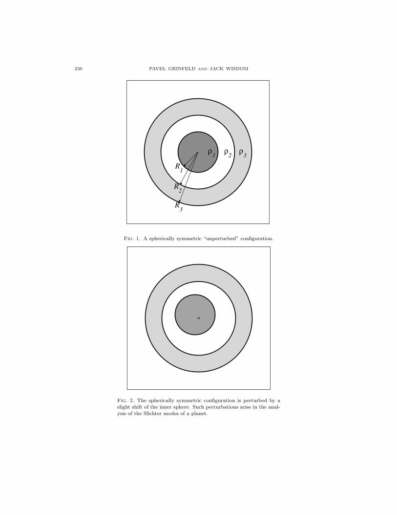
Fig. 1. A spherically symmetric “unperturbed” configuration.

Fig. 2. The spherically symmetric configuration is perturbed by aslight shift of the inner sphere. Such perturbations arise in the anal-ysis of the Slichter modes of a planet.

GRAVITATIONAL POTENTIAL FOR NEAR-SPHERICAL GEOMETRIES 231

Fig. 3. An ellipsoidal perturbation of the spherically symmetric con-figuration. Such perturbations find applications in the analysis of thelibrational modes of an ellipsoidal planet. Note that the inner spherecan be arbitrarily turned relative to the shell.

Fig. 4. An arbitrary small perturbation of the spherically symmetric

configuration. Such perturbations may arise in the study of phasetransformations at the inner core boundary of a planet.


The presented analysis has a number of geophysical applications:a. The study of Slichter modes of the inner core. First studied in 1961 [9] by Slichter,

the modes refer to the translational motion of the inner core of a planet with respectto the outer core and the mantle. Busse [1] presented an analytical treatment of thisproblem in which he treated the constituents of the planet as constant density (Figure1). A small translational displacement of the inner core (Figure 2) can be treated as asmall boundary perturbation of the unperturbed spherical configuration.

b. Libration of the inner core. An inner core and a mantle which are slightly ellipsoidal(Figure 3) are coupled by a gravitational torque that is roughly proportional to theellipticities. As a result, the two parts of the planet oscillate about a stable equilibriumconfiguration. Because the product of the (small) ellipticities is involved, the effect issecond order and requires a second order perturbation analysis.

c. Phase transformations at the inner core boundary. It is a well-accepted hypothesisthat the matter at the inner core - outer core boundary undergoes phase transformations[4]. If the inner core is no longer assumed rigid, then potentially arbitrary deformationsof the interface may occur, as illustrated in the exaggerated Figure 4, and a techniqueflexible enough to analyze such deformations is required.

2. Methodology.2.1. A word about our notation. Throughout the paper we adhere to the indicial no-

tation of tensor calculus, [7], [6], [12]. In our experience, this language is best for thecalculus of moving surfaces outlined in the Appendix. For the sake of consistency we useindicial expressions such as N i∇iψ even where the more conventional N ·∇ψ would havebeen sufficient.

2.2. Evolution of geometries and the power series. The gravitational potential field isdetermined by the distribution of mass densities. Since we consider piecewise constantdensities, the potential field is essentially determined by the geometry of the configura-tion. We suppose that the geometry Ω′, for which the potential field is to be computed, isclose to a spherically symmetric configuration Ω. Then the desired gravitational potentialψ′ (z) for Ω′ is close to ψ0 (z) for Ω. The letter z indicates a point in the three-dimensionalspace.

We imagine a smooth evolution Ω (τ ) of Ω into Ω′ indexed by a time-like parameter τ

(sometimes conveniently thought of as having dimensions of time) such that

Ω (0) = Ω, (1)

Ω (1) = Ω′. (2)

The gravitational potential ψ also undergoes a smooth evolution ψ (τ, z) such that

ψ (0, z) = ψ0 (z) , (3)

ψ (1, z) = ψ′ (z) . (4)

We approximate ψ′ (z) by the first n terms of the power series

ψ′ (z) ≈ ψ0 (z) +∂ψ (τ, z)

∂τ

∣∣∣∣τ=0

+12

∂2ψ (τ, z)∂τ2

∣∣∣∣τ=0

+ ... +1

N !∂Nψ (τ, z)

∂τN

∣∣∣∣τ=0

(5)


and calculate the first three terms explicitly. Note that by letting ∆τ = 1, we considerslow evolutions over a finite period of time rather than an equivalent scenario with finitevelocities over a short period of time.

2.3. Two approaches to the problem. Our task is to compute ∂nψ/∂τn at τ = 0. At agiven time τ , the potential is given by the conceptual integral

ψ (τ, z) = −∫

Ω

ρ (τ, z∗)Distance (z, z∗)

dΩ∗, (6)

where ρ (τ, z) is the imaginary evolution of density distribution. This integral can in prin-ciple be differentiated with respect to τ to obtain ∂ψn/∂τn. Since this approach requiresa complicated analysis of integrals with singularities, we prefer a different approach basedon Poisson’s equation.

Away from the surfaces of density discontinuities, the gravitational potential ψ satisfiesPoisson’s equation

∇i∇iψ = 4πGρ. (7)

In addition, ψ vanishes at infinity and is finite everywhere. Finally, across the interfacesS of density discontinuities, ψ is continuous along with its derivatives

[ψ]S = 0, (8)

N i [∇iψ]S = 0, (9)

where[X]S (10)

stands for the jump in quantity X across the surface S. We require continuity onlyfor the normal derivatives since the continuity of tangential derivatives follows from thecontinuity of ψ.

2.4. Outline of the procedure. We start by calculating the unperturbed potential ψ0 (r)for the initial domain Ω. Since Ω is spherically symmetric, a sphere of radius R in ourcase, this is a straightforward task. We then derive a system of equations for ∂nψ/∂τn

by repeatedly differentiating (or perturbing) the system (7)–(9) with respect to τ . Dif-ferentiating the bulk condition (7) n times yields

∇i∇i∂nψ

∂τn= 0. (11)

The derivative of the right-hand side of (7) vanishes since ρ is presumed piecewise con-stant.

The differentiation of the boundary conditions (8) and (9) is far more challenging andrequires an application of the so-called δ/δτ -derivative, a key operation in the calculusof moving surfaces (see the Appendix).

The perturbed system needs to be solved for the initial configuration since the powerseries (5) requires the values of ∂nψ/∂τn at τ = 0. The spherical symmetry of the initialconfiguration allows us to solve the resulting systems by separation of variables.

We consider a single domain of density ρ. More complicated geometries with piecewiseconstant densities can be obtained by superimposing solid domains. For example, aplanet with an inner core of density ρ1, an outer core of density ρ2 and a mantle of


density ρ3 can be represented as a sphere of radius ρ3 with a smaller sphere (outer core)of density ρ2 − ρ3 and an even smaller sphere (inner core) of density ρ1 − ρ2.

For a sphere of radius R and density ρ, the unperturbed potential ψ0 (z) is given by

ψ0 (r) = 4πGρR2

3

⎧⎪⎨⎪⎩

12

(rR

)2 − 32 , z < Ω,

−(

rR

)−1, z > Ω,

(12)

where z < Ω and z > Ω is a shorthand notation for “points inside Ω” and “points outsideΩ”.

3. First perturbation of the potential.3.1. Solution of Laplace’s equation for a sphere. We noted that ∂nψ/∂τn satisfies

Laplace’s equation in R3, i.e. ∂nψ/∂τn is harmonic. Here, we present the general

solution for the Laplace equation in R3 that is finite at the origin, vanishes at infinity,

and satisfies the given boundary condition on the sphere of radius R.Suppose that χ is a harmonic function

∇i∇iχ = 0 (13)

and that, in addition to being finite at the origin and zero at infinity, χ satisfies thefollowing discontinuity conditions across S, the boundary of Ω:

[χ]S = J, (14a)

N i [∇iχ]S =H

R. (14b)

Both J and H are determined by the evolution Ω (τ ), and the factor of R−1 was intro-duced for nondimensionalization. If the fields J and H are represented as a series inspherical harmonics Ylm (θ, φ)

J = J lmYlm (θ, φ) , (15a)

H = H lmYlm (θ, φ) , (15b)

then χ is given by

χ (r, θ, φ) =

(l+1)Jlm+Hlm

2l+1

(rR

)l, z < Ω

−lJlm+Hlm

2l+1

(rR

)−l−1, z > Ω

∣∣∣∣∣Ylm (θ, φ) . (16)

We usually prefer complex spherical harmonics Ylm (θ, φ) that are normalized to unityon the unit sphere ∫

|r|=1

Yl1m1 (θ, φ)Y ∗l2m2

(θ, φ) dS = δl1l2δm1m2 ,

where ∗ means complex conjugation.As we compute successive perturbations of the system (7)–(9) we obtain Laplace sys-

tems of the type (13)–(14b), each with its own H and J . Denote the H and J appearing


in the n-th perturbation by Jn and Hn and their spherical harmonic expansion coeffi-cients by H lm

n and J lmn . The power series approximation of the perturbation ∆ψ (r, θ, φ)

of ψ (r, θ, φ) (5) is then given by

∆ψ (r, θ, φ) ≈N∑

n=1

⎧⎨⎩

(l+1)Jlmn +Hlm

n

(2l+1)n!

(rR

)l, z < Ω

−lJlmn +Hlm

n

(2l+1)n!

(rR

)−l−1, z > Ω

∣∣∣∣∣∣Ylm (θ, φ) . (17)

The task that remains is to determine the surface fields Jn and Hn and to represent themwith respect to the spherical harmonics.

3.2. The δδτ -derivative and the interface velocity C. This paper relies heavily on the

calculus of moving surfaces, whose concise but complete exposition can be found in theAppendix. This section briefly introduces the main concepts, enabling the reader to seethe big picture presented in the following section while using the Appendix as a reference.

The two primary concepts on the calculus of moving surfaces is the δ/δτ -derivativeand the interface velocity C. In the following sections, the boundary conditions for thepotential field perturbations are stated only in terms of this operator and this quan-tity, plus the stationary surface fields such as the mean curvature. Therefore, while thederivation of the perturbation equations requires the knowledge of the calculus of movingsurfaces, the interpretation of the resulting equations only requires the concepts introducedin this section.

Consider a one parameter family of curves Sτ indexed by a time-like parameter τ . Thefamily Sτ can also be thought of as a time evolution of a single curve S. Let T (τ, Sτ ) be ascalar field defined on Sτ , so T not only changes its values with time but also experiencesa change in its domain of definition.

We present a geometric definition of the δ/δτ -derivative at a point ξ on the surfaceSτ at time τ , illustrated in Figure 5. Consider two locations of the surface Sτ and Sτ∗

at nearby times τ and τ∗. Draw the straight line orthogonal to Sτ passing through thepoint ξ. Mark the point ξ∗, where this straight line intersects Sτ∗ . Define

δT (τ, ξ)δτ

= limτ∗→τ

T (τ∗, ξ∗) − T (τ, ξ)τ∗ − τ

. (18)

An equivalent algebraic definition of the δ/δτ -derivative of a scalar is given by equation(108) of the Appendix. A general definition applicable to tensors of arbitrary shape isgiven by equation (111).

Let ∆z be the vector connecting the point ξ to the point ξ∗. Then the velocity of theinterface C (also known as the normal velocity) is defined as

C = limτ∗→τ

∆z · Nτ∗ − τ

, (19)

where N is the unit normal to the surface Sτ . By construction, ∆z is aligned with N,and the dot indicates that the sign of C depends on the choice of the normal. ObviouslyC is a scalar, and it is called “velocity” rather than “speed” because the normal directionis implied.


ξ,Tτ(ξ)

ξ*,Tτ*(ξ*)

Fig. 5. Geometric definition of the δ/δτ -derivative as applied to ascalar field T defined at time τ on the surface Sτ .

If z is the radius vector with respect to an arbitrary origin, then the definition of C

(19) can be rewritten as

C =δzδτ

·N.

The velocity field C completely determines the evolution of the interface, much likeprescribing the velocity field of a fluid completely determines its flow, with one significantdifference. In the flow of a fluid, the trajectories of individual particles are usually ofinterest and the velocity field allows one to determine the flow. The velocity C, on theother hand, describes the motion of the surface as a geometric object not keeping trackof individual points.

3.3. The first perturbation ∂ψ/∂τ . The perturbed bulk equation is obtained simplyby differentiating Poisson’s equation with respect to τ :

∇i∇i∂ψ

∂τ= 0. (20)

Since ρ is constant, the would-be right-hand side 4πG ∂ρ∂τ vanishes. The effect of the

variation in the mass density is instead captured by the boundary conditions.Taking a δ/δτ -derivative (see the Appendix) of

[∂ψ∂τ

]S

= 0 we get

0 =δ [ψ]S

δτ=[δψ

δτ

]S

, (21)

by eqn. (112) =[∂ψ

∂τ

]S

+ CN i [∇iψ]S , (22)

where C is the velocity of the interface defined above.Since the jump in the normal derivative of ψ vanishes, so does [∂ψ/∂τ ]S :

[∂ψ

∂τ

]S

= 0. (23)


Taking the δ/δτ derivative of the second boundary condition, we have

0 =δ(N i [∇iψ]S

)δτ

=

[δ(N i∇iψ

)δτ

]S

, (24a)

∗ =δN i

δτ[∇iψ]S + N i

[δ∇iψ

δτ

]S

, (24b)

& = −ziα∇αC [∇iψ]S + N i

[∇i

∂ψ

∂τ

]S

+ CN iN j [∇i∇jψ]S . (24c)

∗Product Rule (24d)&By eqns. (114e) and (112) (24e)

Since ∇iψ is orthogonal to the interface at τ = 0, the product ziα∇iψ vanishes on both

sides of the interface, and we have

N i

[∇i

∂ψ

∂τ

]S

= −CN iN j [∇i∇jψ]S . (25)

It can be shown for a continuous function ψ with continuous derivatives that

[∇i∇jψ]S =(NkN l [∇k∇lψ]S

)NiNj . (26)

In other words, the nine entries of [∇i∇jψ]S share a single degree of freedom (ratherthan six for an arbitrary function). Raising one of the indices and contracting, we get[∇i∇iψ

]S

= 4πG [ρ]S . Therefore, the second boundary condition can be rewritten as

N i

[∇i

∂ψ

∂τ

]S

= −4πGCρ. (27)

Summarizing, the perturbed potential ∂ψ/∂τ is governed by

∇i∇i∂ψ

∂τ= 0, z ∈ Ω, (28)[

∂ψ

∂τ

]S

= 0, (29)

N i

[∇i

∂ψ

∂τ

]S

= −4πGCρ. (30)

Therefore, the “jump” function J1 and the “hop” function H1 are given by

J1 = 0, (31a)

H1 = −4πGRCρ. (31b)

Let us now represent C as a series in spherical harmonics in a way similar to equations(15b) and (15a) except with an additional parameter R for nondimensionalization:

C = RClmYlm (θ, φ) . (32)

As C is determined by the evolution Ω (τ ), so are the Clm. We think of the Clm asthe collection of small parameters that represent the given perturbation, and all relevantexpressions are given in terms of the Clm. Below, we shall explicitly calculate the Clm

for two specific perturbations of the sphere: a radial perturbation that preserves thesymmetry of the system and an ellipsoidal perturbation.


Given equations (31a) and (31b), the coefficients J lm1 and H lm

1 are easy to determine:

J lm1 = 0, (33a)

H lm1 = −4πGR2ρClm. (33b)

We have thus obtained the first order approximation to the gravitational potential:

∆ψ (r, θ, φ) ≈ −4πGρR2Clm

2l + 1

(rR

)l , z < Ω,(rR

)−l−1, z > Ω,

Ylm (θ, φ) . (34)

4. Second and third perturbations. The system of equations for ∂2ψ/∂τ2 is ob-tained by repeating the steps of the previous section, i.e. by differentiating equations(28)–(30) we respect to τ :

∇i∇i∂2ψ

∂τ2= 0, z ∈ Ω, (35)[

∂2ψ

∂τ2

]S

= 4πGρC2, (36)

N i

[∇i

∂2ψ

∂τ2

]S

= −4πGρδC

δτ+ 4πGρC2Bα

α ,

where Bαa is the mean curvature (102) which, for a sphere of radius R, equals −2/R. We

rewrite the last boundary condition as

N i

[∇i

∂2ψ

∂τ2

]S

= −4πGρ

(2C2

R+

δC

δτ

). (37)

J2 and H2 are therefore given by

J2 = 4πGρC2, (38a)

H2 = −4πGρ

(2C2 + R

δC

δτ

). (38b)

The surface fields J2 and H2 cannot be as easily decomposed in spherical harmonics asJ1 (which was zero) and H1 (which was directly proportional to C). Therefore, for agiven perturbation they need to be explicitly computed and independently expressed inspherical harmonics. Below we perform this task for radial and ellipsoidal perturbations.

Finally, we present the system for ∂3ψ/∂τ3, which is obtained analogously to ∂ψ/∂τ

and ∂2ψ/∂τ2:

∇i∇i∂2ψ

∂τ2= 0, z ∈ Ω, (39a)[

∂2ψ

∂τ2

]S

= 4πGρ

(3C

δC

δτ− C3Bα

α

), (39b)

N i

[∇i

∂2ψ

∂τ2

]S

= −4πGρ

(δ2Cδτ2 − 3C δC

δτ Bαα − 3C2∇α∇αC − ...

... − 4C∇αC∇αC − C3Bαβ Bβ

α + C3BααBβ

β

), (39c)


where (having substituted Bαα = −2/R and Bα

β Bβa = 2/R2)

J3 = 4πGρ

(3C

δC

δτ+

2C3

R

), (40a)

H3 = −4πGρ

(R δ2C

δτ2 + 6C δCδτ − 3RC2∇α∇αC − ...

... − 4RC∇αC∇αC + 2C3

R

). (40b)

We reiterate that the perturbation equations are started only in terms of the operatorδ/δτ and the velocity field C along with the stationary characteristics of the surface suchas the mean curvature Bα

α and the trace of the third groundform Bαβ Bβ

α.

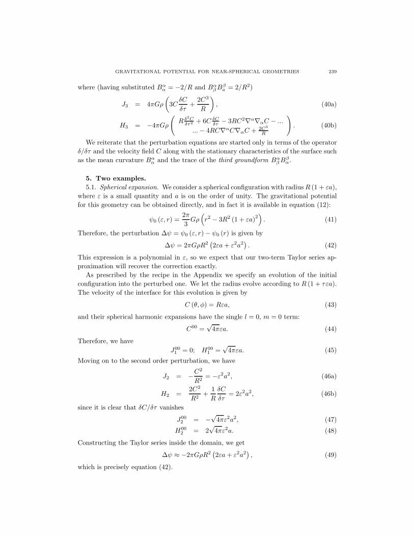
5. Two examples.5.1. Spherical expansion. We consider a spherical configuration with radius R (1 + εa),

where ε is a small quantity and a is on the order of unity. The gravitational potentialfor this geometry can be obtained directly, and in fact it is available in equation (12):

ψ0 (ε, r) =2π

3Gρ

(r2 − 3R2 (1 + εa)2

). (41)

Therefore, the perturbation ∆ψ = ψ0 (ε, r) − ψ0 (r) is given by

∆ψ = 2πGρR2(2εa + ε2a2

). (42)

This expression is a polynomial in ε, so we expect that our two-term Taylor series ap-proximation will recover the correction exactly.

As prescribed by the recipe in the Appendix we specify an evolution of the initialconfiguration into the perturbed one. We let the radius evolve according to R (1 + τεa).The velocity of the interface for this evolution is given by

C (θ, φ) = Rεa, (43)

and their spherical harmonic expansions have the single l = 0, m = 0 term:

C00 =√

4πεa. (44)

Therefore, we haveJ00

1 = 0; H001 =

√4πεa. (45)

Moving on to the second order perturbation, we have

J2 = −C2

R2= −ε2a2, (46a)

H2 =2C2

R2+

1R

δC

δτ= 2ε2a2, (46b)

since it is clear that δC/δτ vanishes

J002 = −

√4πε2a2, (47)

H002 = 2

√4πε2a. (48)

Constructing the Taylor series inside the domain, we get

∆ψ ≈ −2πGρR2(2εa + ε2a2

), (49)

which is precisely equation (42).


5.2. Ellipsoidal perturbation. We now turn to the computation of the potential insidea near-spherical ellipsoidal domain. The potential outside this domain can be computedanalogously, but the results are not presented here for consideration of space.

The gravitational potential of a near-spherical ellipsoid can be estimated to any orderby a technique originally proposed by Migdal [8], [5] for the analysis of the energy splittingof a quantum particle trapped in an ellipsoidal cavity. Migdal’s technique is simplerthan ours (although not shorter!) for lower order perturbations and can be used for anindependent verification of our results.

The gravitational correction inside a slightly ellipsoidal shell was also calculated tosecond order in [10].

The boundary S is an ellipsoid with semi-axes R (1 + εa), R (1 + εb), R (1 + εc). Asbefore, we start by specifying the evolution from Ω0 (a sphere of radius R) to Ω1 (ourellipsoid): ⎡

⎣ z1

z2

z3

⎤⎦ = R

⎡⎣ (1 + τa) sin θ cos φ

(1 + τb) sin θ sin φ

(1 + τc) cos θ

⎤⎦ . (50)

5.2.1. Computing C. The marker velocity vi (107a) is given by

vi =∂zi

∂τ= R

⎡⎣ a sin θ cos φ

b sin θ sin φ

c cos θ

⎤⎦ , (51)

and the velocity C of the boundary at τ = 0 is constructed by projecting the markervelocity onto the unperturbed normal N i = (a sin θ cos φ, b sin θ sin φ, c cos θ):

C|τ=0 = R(a sin2 θ cos2 φ + b sin2 θ sin2 φ + c cos2 θ

). (52)

This expression is easy to represent in terms of Ylm as in equation (32), since only a fewterms are nonzero:

C00 =

√4π

9(a + b + c) , (53a)

C2m =

⎡⎢⎢⎢⎢⎢⎢⎢⎣

√2π15 (a − b)

0

−√

4π45 (a + b − 2c)

0√2π15 (a − b)

⎤⎥⎥⎥⎥⎥⎥⎥⎦

. (53b)

These coefficients can practically be obtained from equation (52) in a number of ways.One is by integration:

Clm =1R

∫ π

−π

∫ π

0

C (θ, φ)Y ∗lm (θ, φ) sin θdθdφ, (54)

where ∗ stands for complex conjugation.


Alternatively, one can expand the harmonic series for C (32) as a single trigonometricpolynomial and form a linear system for Clm by matching up the terms of the trigono-metric polynomials with the explicit expression (52) for C.

5.3. First order coefficients. Decomposing J1 = 0 and H1 = C/R, defined by equa-tions (14a), (14b), with respect to spherical harmonics yields the following coefficients(15a), (15b):

(l + 1)J lm1 + H lm

1

−4πGR2ρ

∣∣∣∣l=0

=−lJ lm

1 + H lm1

−4πGR2ρ

∣∣∣∣l=0

=

√4π

9(a + b + c) , (55a)

(l + 1)J lm1 + H lm

1

−4πGR2ρ

∣∣∣∣l=2

=−lJ lm

1 + H lm1

−4πGR2ρ

∣∣∣∣l=2

=

⎡⎢⎢⎢⎢⎢⎢⎢⎣

√2π15 (a − b)

0

−√

4π45 (a + b − 2c)

0√2π15 (a − b)

⎤⎥⎥⎥⎥⎥⎥⎥⎦

. (55b)

5.3.1. Computing δC/δτ . According to the definition of the δ/δτ -derivative (108), wehave

δC

δτ=

∂C (τ, θ, φ)∂τ

− vizαi ∇αC. (56)

The term ∂C/∂τ contains a partial derivative of the normal N i with respect to τ . Thiswould be a very cumbersome computation, given the definition of the normal in equation(95). It can be avoided by utilizing equations (111) and (114e) to eliminate the ∂N i/∂τ

term. The resulting expression is

δC

δτ= −viz

iα

(Nk∇αvk + ∇αC

). (57)

The shift tensor ziα (87) is given by

ziα = R

⎡⎣ cos θ cos φ − sin θ sin φ

cos θ sin φ sin θ cos φ

− sin θ 0

⎤⎦ . (58)

Since C is a scalar, the surface gradient (97) of C coincides with the ordinary gradient:

∇αC = R

[ (12a − 1

2b)sin 2θ cos 2φ −

(c − 1

2a − 12b)sin 2θ

− (a − b) sin2 θ sin 2φ

]. (59)

The surface gradient of the marker velocity coincides with the ordinary gradient, since aCartesian metric is used in the embedding space:

∇αvi = R

⎡⎣ cos θ cos φ − sin θ sin φ


− sin θ 0

⎤⎦ . (60)


Putting everything together we obtain the following expression:

δC

δτ= −


b sin θ sin φ

c cos θ

⎤⎦

T ⎡⎣ cos θ cos φ − sin θ sin φ


− sin θ 0

⎤⎦[ 1 0

0 sin2 θ

]−1[

∂C∂θ∂C∂φ

]

−


b sin θ sin φ

c cos θ

⎤⎦

T ⎡⎣ cos θ cos φ − sin θ sin φ


− sin θ 0

⎤⎦[ 1 0

0 sin2 θ

](61a)

×

⎡⎣ a cos θ cos φ −a sin θ sin φ

b cos θ sin φ b sin θ cos φ

−c sin θ 0

⎤⎦

T ⎡⎣ sin θ cos φ

sin θ sin φ

cos θ

⎤⎦ .

5.3.2. Second order coefficients. The following equations summarize the values for(l + 1) J lm

n + H lmn and −lJ lm

n + H lmn , which were obtained using Mathematica [13]:

(l + 1)J lm2 + H lm

2

4πGR2ρ

∣∣∣∣l=0

=215

√π(3a2 + 3b2 + 3c2 − 8ab − 8bc − 8ca

), (62a)

(l + 1)J lm2 + H lm

2

4πGR2ρ

∣∣∣∣l=2

=

⎡⎢⎢⎢⎢⎢⎣

√30π

105 (a − b) (9a + 9b − 4c)0

− 2√

5π105

(9a2 + 9b2 − 18c2 − 8ab + 4bc + 4ca

)0√

30π105 (a − b) (9a + 9b − 4c)

⎤⎥⎥⎥⎥⎥⎦ , (62b)

−lJ lm2 + H lm

2

4πGR2ρ

∣∣∣∣l=0

= −4√

π

3(a b + bc + ca) , (63a)

−lJ lm2 + H lm

2

−4πGR2ρ

∣∣∣∣l=2

=

⎡⎢⎢⎢⎢⎢⎣

√30π15 (a − b) (3a + 3b + 2c)

0− 2

√5π

15

(3a2 + 3b2 − 6c2 + 4ab − 2bc − 2ca

)0√

30π15 (a − b) (3a + 3b + 2c)

⎤⎥⎥⎥⎥⎥⎦ , (63b)

−lJ lm2 + H lm

2

4πGR2ρ

∣∣∣∣l=4

=

⎡⎢⎢⎢⎢⎢⎢⎢⎢⎢⎢⎢⎢⎢⎢⎣

−3√

70π35 (a − b)2

06√

10π35 (a − b) (a + b − 2c)

0− 6

√π

35

(3a2 + 3b2 + 8c2 + 2ab − 8bc − 8ca

)0

6√

10π35 (a − b) (a + b − 2c)

0− 3

√70π

35 (a − b)2

⎤⎥⎥⎥⎥⎥⎥⎥⎥⎥⎥⎥⎥⎥⎥⎦

. (63c)

Interestingly, according to equation (62b) there is no contribution from the l = 4 harmon-ics inside the ellipsoid, consistent with the fact that inside the ellipsoid with arbitrarysemi-axes the potential is a linear function of x2, y2, and z2, each of which can berepresented as a linear combination of r2Y2m.


5.3.3. Third order coefficients. Finally, we present the coefficients for the third orderperturbation:

(l + 1) J lm3 + H lm

3

4πGR2ρ

∣∣∣∣l=0

= −8√

π

35(a + b − 2 c) (2 a − b − c) (a − 2 b + c) , (64a)

(l + 1) J lm3 + H lm

3

4πGR2ρ

∣∣∣∣l=2

=

⎡⎢⎢⎢⎢⎢⎢⎢⎢⎢⎢⎢⎢⎢⎣

−27

√2 π15 (a − b)

(8 a2 + 8 b2 − 5 c2

+12 a b − b c − a c

)0

421

√π5

⎛⎝ 8 a3 + 8 b3 − 16 c3

−6 a2 b − 6 a b2 − 3 a c2 − 3 b c2

+9 b2 c + 9 a2 c

⎞⎠

0

−27

√2 π15 (a − b)

(8 a2 + 8 b2 − 5 c2

+12 a b − b c − a c

)

⎤⎥⎥⎥⎥⎥⎥⎥⎥⎥⎥⎥⎥⎥⎦

, (64b)

−lJ lm3 + H lm

3

4πGR2ρ

∣∣∣∣l=0

= 4√

π a b c, (65a)

−lJ lm3 + H lm

3

4πGR2ρ

∣∣∣∣l=2

=

⎡⎢⎢⎢⎢⎢⎢⎢⎢⎣

−√

6 π5 (a − b)

(a2 + 4 a b + b2 + 3 a c + 3 b c

)0

2√

π5

(a3 + 3 a2 b + 3 a b2 + b3

+3 a2 c + 3 b2 c − 6 a c2 − 6 b c2 − 2 c3

)0

−√

6 π5 (a − b)

(a2 + 4 a b + b2 + 3 a c + 3 b c

)

⎤⎥⎥⎥⎥⎥⎥⎥⎥⎦

, (65b)

−lJ lm3 + H lm

3

4πGR2ρ

∣∣∣∣l=4

=

⎡⎢⎢⎢⎢⎢⎢⎢⎢⎢⎢⎢⎢⎢⎢⎢⎢⎢⎢⎢⎢⎢⎢⎢⎢⎣

−9 (a − b)2 (2 a + 2 b + c)√

2 π35

0

187

√2 π5 (a − b)

(2 a2 + 2 b2 − 3 c2

+3 a b − 2 a c − 2 b c

)0

−1835

√π

⎛⎝ 6 a3 + 6 b3 + 16 c3 + 6 a2 b + 6 a b2

−9 a2 c − 9 b2 c − 4 a c2 − 4 b c2

−14 a b c

⎞⎠

0

187

√2 π5 (a − b)

(2 a2 + 2 b2 − 3 c2

+3 a b − 2 a c − 2 b c

)0

−9√

2 π35 (a − b)2 (2 a + 2 b + c)

⎤⎥⎥⎥⎥⎥⎥⎥⎥⎥⎥⎥⎥⎥⎥⎥⎥⎥⎥⎥⎥⎥⎥⎥⎥⎦

, (65c)


−lJ lm3 + H lm

3

4πGR2ρ

∣∣∣∣l=6

=

⎡⎢⎢⎢⎢⎢⎢⎢⎢⎢⎢⎢⎢⎢⎢⎢⎢⎢⎢⎢⎢⎢⎢⎢⎢⎢⎢⎢⎢⎢⎢⎢⎢⎣

−√

143 π21 (a − b)3

0√26 π7 (a − b)2 (a + b − 2 c)

0

−√

13 π105 (a − b)

(5 a2 + 6 a b + 5 b2

−16 a c − 16 b c + 16 c2

)0

221

√13 π (a + b − 2 c)

(5 a2 + 5 b2 + 8 c2

−2 a b − 8 a c − 8 b c

)0

−√

13 π105 (a − b)

(5 a2 + 6 a b + 5 b2

−16 a c − 16 b c + 16 c2

)0√

26 π7 (a − b)2 (a + b − 2 c)

0

−√

143 π21 (a − b)3

⎤⎥⎥⎥⎥⎥⎥⎥⎥⎥⎥⎥⎥⎥⎥⎥⎥⎥⎥⎥⎥⎥⎥⎥⎥⎥⎥⎥⎥⎥⎥⎥⎥⎦

. (65d)

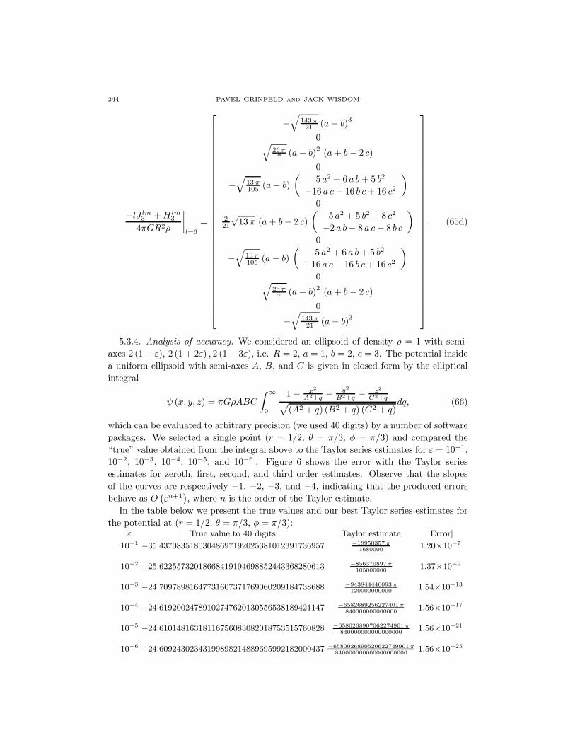
5.3.4. Analysis of accuracy. We considered an ellipsoid of density ρ = 1 with semi-axes 2 (1 + ε), 2 (1 + 2ε) , 2 (1 + 3ε), i.e. R = 2, a = 1, b = 2, c = 3. The potential insidea uniform ellipsoid with semi-axes A, B, and C is given in closed form by the ellipticalintegral

ψ (x, y, z) = πGρABC

∫ ∞

0

1 − x2

A2+q − y2

B2+q − z2

C2+q√(A2 + q) (B2 + q) (C2 + q)

dq, (66)

which can be evaluated to arbitrary precision (we used 40 digits) by a number of softwarepackages. We selected a single point (r = 1/2, θ = π/3, φ = π/3) and compared the“true” value obtained from the integral above to the Taylor series estimates for ε = 10−1,10−2, 10−3, 10−4, 10−5, and 10−6.. Figure 6 shows the error with the Taylor seriesestimates for zeroth, first, second, and third order estimates. Observe that the slopesof the curves are respectively −1, −2, −3, and −4, indicating that the produced errorsbehave as O

(εn+1

), where n is the order of the Taylor estimate.

In the table below we present the true values and our best Taylor series estimates forthe potential at (r = 1/2, θ = π/3, φ = π/3):

ε True value to 40 digits Taylor estimate |Error|10−1 −35.43708351803048697192025381012391736957 −18950357 π

16800001.20×10−7

10−2 −25.62255732018668419194698852443368280613 −856370897 π105000000

1.37×10−9

10−3 −24.70978981647731607371769060209184738688 −943844446093 π120000000000

1.54×10−13

10−4 −24.61920024789102747620130556538189421147 −6582689256227401 π840000000000000

1.56×10−17

10−5 −24.61014816318116756083082018753515760828 −6580268907062274901 π840000000000000000

1.56×10−21

10−6 −24.60924302343199898214889695992182000437 −6580026890520622749901 π840000000000000000000

1.56×10−25


10-6

10- 5

10- 4

10- 3

10- 2

10-25

10-20

10-15

10-10

10-5

100

ε

Err

or

Fig. 6. The error in the Taylor series estimate for ε = 10−2, 10−3,10−4, 10−5, 10−6. The four curves correspond to the Taylor serieswith zero, one, two, and three terms.

The ellipticity of the Earth is roughly on the order of 10−2. Since the density ofthe Earth varies with distance from the center, our technique is not directly applicable.However, an adaptation of our technique would be applicable, and Figure 6 indicatesthat the second order estimate will produce a relative error on the order of 5 × 10−11.

6. First order perturbation for a triaxial planet. This section is concerned withan example that has a number of geophysical applications related to the dynamics of theinner core and also shows how to apply the obtained expressions to composite geometries.Suppose that the configuration (before the perturbation) consists of an inner core Ω1 ofradius R1 and density ρ1, an outer core Ω2 of radius R2 and density ρ2, and a mantleΩ3 of radius R3 and density ρ3. This configuration can be equivalently represented bythree superimposed spheres: one of radius R3 and density ρ3, another of radius R2 anddensity ρ2 − ρ3, and a third one of radius R1 and density ρ1 − ρ2.

We construct the estimates for the resulting potential by adjusting expressions for theunperturbed potential (12) and the first order perturbation (34) to each of the domainsand then combining them. In order to make equations (12) and (34) appear more generic,introduce a radius R∗ and a density ρ∗. Also, define the dimensionless densities n and


radii Qn:

n =ρn

ρ∗, Qn =

Rn

R∗, (67)

and a convenient quantity Ψ∗ that has dimensions of gravitational potential:

Ψ∗ =4π

3Gρ∗R

2∗. (68)

Consistent with the definition (10), let []1 = 1 − 2, []2 = 2 − 3, and []3 = 3.6.1. The unperturbed potential. The unperturbed potential for a single domain (say

Ω1), equation (12), can now be rewritten as

ψ0 (r) = Ψ∗

⎧⎪⎨⎪⎩

[]12

(r

R∗

)2

− 32 []1 Q2

1, z < Ω1,

− []1 Q31

(r

R∗

)−1

, z > Ω1,

and the combined expression is easily obtained by replacing the subscript of 1 with 2and 3:

ψ0 (r) = Ψ∗

⎧⎪⎪⎪⎪⎪⎪⎪⎪⎪⎪⎪⎪⎪⎪⎨⎪⎪⎪⎪⎪⎪⎪⎪⎪⎪⎪⎪⎪⎪⎩

[]12

(r

R∗

)2

− 32 []1 Q2

1, z < Ω1,

− []1 Q31

(r

R∗

)−1

, z > Ω1,

+[]22

(r

R∗

)2

− 32 []2 Q2

2, z < Ω2,

− []2 Q32

(r

R∗

)−1

, z > Ω2,

+[]32

(r

R∗

)2

− 32 []3 Q2

3, z < Ω3,

− []3 Q33

(r

R∗

)−1

, z > Ω3.

Rewriting the sum in a single expression, we get

ψ0 (r) = Ψ∗

⎧⎪⎪⎪⎪⎪⎪⎪⎨⎪⎪⎪⎪⎪⎪⎪⎩

12

(r

R∗

)2

+ A1, z < Ω1,

22

(r

R∗

)2

+ A2 + B2

(r

R∗

)−1

, Ω1 < z < Ω2,

32

(r

R∗

)2

+ A3 + B3

(r

R∗

)−1

, Ω2 < z < Ω3,

B4

(r

R∗

)−1

, Ω3 < z,

(69)

where

⎡⎢⎢⎢⎢⎢⎢⎢⎣

A1

A2

A3

B2

B3

B4

⎤⎥⎥⎥⎥⎥⎥⎥⎦

=

⎡⎢⎢⎢⎢⎢⎢⎢⎢⎢⎢⎢⎢⎢⎢⎢⎢⎢⎣

−32 []1 Q2

1 − 32 []2 Q2

2 − 32 []3 Q2

3

−32 []2 Q2

2 − 32 []3 Q2

3

−32 []3 Q2

3

− []1 Q31

− []1 Q31 − []2 Q3

2

− []1 Q31 − []2 Q3

2 − []3 Q33

⎤⎥⎥⎥⎥⎥⎥⎥⎥⎥⎥⎥⎥⎥⎥⎥⎥⎥⎦

. (70)


6.2. The first order perturbation. We assume that each of the three domains Ωn isperturbed in its own way according to Cn and that each Cn is represented as a series inspherical harmonics

Cn = RnClmn Ylm.

We first rewrite the first order perturbation for a single domain (say Ω1) as

∆ψ (r, θ, φ) ≈ − 3Ψ∗2l + 1

⎧⎪⎨⎪⎩

[]1 Q−l+21

(r

R∗

)l

Clm1 , z < Ω1,

[]1 Ql+31

(r

R∗

)−l−1

Clm1 , z > Ω1,

Ylm (θ, φ) ,

and the combined expression can be obtained similarly to the unperturbed potential:

∂ψ

∂τ(r, θ, φ) = Ψ∗

⎧⎪⎪⎪⎪⎪⎪⎪⎨⎪⎪⎪⎪⎪⎪⎪⎩

Alm1

(r

R∗

)l

, z < Ω1

Alm2

(r

R∗

)l

+ Blm2

(r

R∗

)−l−1

, Ω1 < z < Ω2

Alm3

(r

R∗

)l

+ Blm3

(r

R∗

)−l−1

, Ω2 < z < Ω3

Blm4

(r

R∗

)−l−1

, Ω3 < z

∣∣∣∣∣∣∣∣∣∣∣∣∣Ylm (θ, φ) , (71)

where ⎡⎢⎢⎢⎢⎢⎢⎢⎣

Alm1

Alm2

Alm3

Blm2

Blm3

Blm4

⎤⎥⎥⎥⎥⎥⎥⎥⎦

= − 32l + 1

⎡⎢⎢⎢⎢⎢⎢⎢⎣

Q−l+21 Q−l+2

2 Q−l+23

0 Q−l+22 Q−l+2

3

0 0 Q−l+23

Ql+31 0 0

Ql+31 Ql+3

2 0Ql+3

1 Ql+32 Ql+3

3

⎤⎥⎥⎥⎥⎥⎥⎥⎦

⎡⎣ []1 Clm

1

[]2 Clm2

[]3 Clm3

⎤⎦ . (72)

We have computed a first order correction to the graviational potential of a piecewiseconstant density tri-layer planet for aribtrary small deformations of the three interfaces.Such deformations are typically caused by the planet’s rotation (Earth) or by thermalconvection in the interior of the planet (Mercury). In both cases, the deformations may betreated as ellipsoidal for a number of purposes. Therefore, the resulting corrections to thegravitational field may be obtained by substituting the ellipsoidal expansion coefficientsClm, equations (53a)–(53b), into the expressions for ∂ψ/∂τ, equations (71)–(72). Theresulting estimates are consistent with the estimates obtained by Szeto and Xu in [10]for the gravitational potential inside an ellipsoidal cavity.

7. Appendix: A concise exposition of the δ/δτ -derivative.7.1. Objects defined in a Euclidean space. The radius vector z extends from an arbi-

trarily selected pole O to points in the Euclidean space. In a coordinate system zi (i.e.(z1, z2, z3

)), the radius vector z becomes a (vector-valued) function of zi: z = z

(zi).

This definition overloads the symbol z—it now stands for both an invariant vector fieldand its functional representation. We almost always omit the indices in the argumentsof a function and simply write

z = z (z) , (73)

implying z = z(z1, z2, z3

).


The covariant basis zi is defined at every point in space as

zi =∂z∂zi

. (74)

The covariant basis is a (vector-valued) tensor which can be shown by a simple applicationof the chain rule.

The covariant metric tensor zij is defined as

zij = zi · zj . (75)

Consistent with its name, it is a doubly covariant tensor which follows from the factthat the dot product is a tensor operation. As a matrix it is symmetric and positive(semi-)definite.

When it leads to no confusion, the determinant |zij | (not a tensor) is denoted by z.The permutation tensors zijk and zijk are defined as

zijk =√

zeijk, zijk =1√zeijk, (76)

where

eijk, eijk =

⎧⎨⎩

+1, if i, j, k is a positive permutation,

−1, if i, j, k is a negative permutation,

0, otherwise.(77)

The contravariant metric tensor zij is defined as the matrix inverse of zij :

zijzjk = δk

i . (78)

Linear algebra dictates that contraction by the other index (“commuting” in the languageof LA) also yields δi

j (“Identity” in LA):

zijzki = δk

j . (79)

The tensors zij and zij are used for raising and lowering indices. Raising the secondindex of zij by zjk leads to z·ki , but it also leads to δ·ki ! Therefore, δ and z can be usedinterchangeably (but then δij no longer has the Kronecker interpretation).

The inner product of two vectors a = aizi and b = bizi is given by

a · b = aizi · bizi = zijaibj = aibi = ajb

j . (80)

The contravariant component ai can be extracted by dotting a with zi:

ai = a · zi. (81)

The covariant derivative ∇i, as applied to a typical tensor T j·k, is defined as

∇iTj·k =

∂T j·k (z)∂zi

+ ΓjimTm

·k − ΓmikT j

·m, (82)

where the Christoffel symbol Γijk (not a tensor) is defined as

Γijk =

∂zj

∂zk· zi. (83)


When applied to tensors, the covariant derivative yields tensors of one covariant orderhigher. The covariant derivative reduces to the partial when applied to tensors of or-der zero, or when applied to general tensors in affine coordinate systems. Covariantdifferentiation in Euclidean spaces is commutative

∇i∇j = ∇j∇i (84)

and kills all metrics

∇mzij ,∇mδij ,∇mzij ,∇mz,∇mzi,∇mzi,∇mzijk,∇mzijk = 0. (85)

7.2. Objects defined on embedded surfaces. Consider a surface S given parametricallyin coordinates ξα as

zi = zi (ξ) . (86)

The shift tensor ziα is defined as

ziα =

∂zi

∂ξα. (87)

It is a tensor with respect to both a change of coordinates in space and a change ofcoordinates on the surface.

The covariant basis ξα is defined as

ξα =∂z∂ξα

. (88)

An application of the chain rule gives an alternative expression

ξα = ziαzi (89)

and suggests the interpretation of ziα as a projection operator. Any surface vector a =

aαξα can be decomposed with respect to the spatial basis zi as a = aizi, where ai = ziαaα.

The covariant metric tensor ξαβ is defined as

ξαβ = ξα · ξβ (90)

and is also expressed asξαβ = zijz

iαzj

β, (91)

which (running one sentence ahead) can be alternatively written as

ziαzβ

i = δβα. (92)

The contravariant metric tensor ξαβ is defined as the matrix inverse of ξαβ :

ξαβξβγ = δγα; ξαβξγα = δγ

β . (93)

When it leads to no confusion, the determinant |ξαβ | (not a tensor) is denoted by ξ.The permutation tensors εαβ and εαβ (reusing letter ξ is impossible) are defined as

εαβ =√

ξeαβ , εαβ =1√ξeαβ , (94)

where e12 = −e21 = 1 and e11 = e22 = 0.


The normal N i is defined as

N i =12zijkεαβzα

j zβk . (95)

It is of unit length, N iNi = 1, and is orthogonal to the surface N izαi = 0.

The tensor ziαzα

j is interpreted as the projection onto the surface. This interpretationis firmly justified by the following identity:

ziαzα

j = δij − N iNj . (96)

The covariant derivative ∇γ as applied to a typical tensor T j·α··k·β is defined as

∇γT i·α··j·β =

T i·α··j·β

∂ξγ+ zk

γΓikmTm·α·

·j·β − zkγΓm

kjTi·α··m·β + Γα

γδTi·δ··j·β − Γδ

γβT i·α··j·δ , (97)

where the Christoffel symbol Γαβγ (not a tensor) must now be defined traditionally:

Γαβγ =

12ξαω

(∂ξωγ

∂ξβ+

∂ξωβ

∂ξγ− ∂ξβγ

∂ξω

). (98)

When applied to a surface restriction of a spatial tensor T i·j we have the chain rule

∇αT i·j = zk

α∇kT i·j . (99)

The covariant surface derivative kills many of the metrics (but not the bases):

∇λξαβ , ∇λδβα, ∇λξαβ, ∇λεαβ ,∇λεαβ = 0. (100)

The chain rule tells us that the covariant surface derivatives kills all spatial metrics:

∇γzij ,∇γδij ,∇γzij ,∇γz,∇γzi,∇γzi,∇γzijk,∇γzijk = 0. (101)

The curvature tensor Bαβ is defined as

Bαβ = Ni∇αziβ . (102)

Multiplying both sides by N j and applying the projection formula, we get N jBαβ =

N jNi∇αziβ =

(δji − zγ

i zjγ

)∇αzi

β = ∇αzjβ − zj

γ∇αδγβ . Since the second term is zero, we

obtain the formula for differentiating the shift tensor:

∇αziβ = N iBαβ . (103)

Once again taking the definition of Bαβ and multiplying both sides by zjβ , we get

zjβBαβ = Nizjβ∇αzi

β = −zjβziβ∇αNi =

(−δij + N iNj

)∇αNi = −∇αN j +NjN

i∇αNi.Since N iNi ≡ 1, the second term vanishes and we obtain the formula for differentiatingthe normal

∇αN i = −ziβBαβ . (104)

Gauss’s Theorema Egregium

|B..| ενµεαβ = BανBβµ − BβνBαµ (105)

can be interpreted as saying that the tensor Bαβ has only two degrees of freedom (themean curvature and the intrinsic curvature).


7.3. The δ/δτ -derivative for moving surfaces. Let the motion of the surface Sτ bedescribed by

Sτ : zi = zi (τ, ξ) . (106)

Define the marker velocity vi (not a tensor) and its projection vα onto the surface (alsonot a tensor) as

vi (τ, ξ) =∂zi (τ, ξ)

∂τ, (107a)

vα = zαi vi. (107b)

For a tensor of order zero T , the derivative δTδτ is defined as [11]

δT (τ, ξ)δτ

=∂T (τ, ξ)

∂τ− vα∇αT. (108)

The physical interpretation of this definition is shown in Figure 5.The velocity of the interface C is defined as

C =δzδτ

· N. (109)

It is clear from Figure 5 that δzδτ is normal to the surface, so δz

δτ = CN. We also have

C = viNi. (110)

The definition (108) applies only to scalars and not more general tensors such as ziα and

Bαβ . For an arbitrary tensor T i·α·

·j·β , the definition of δ/δτ -derivative was given in [2]:

δT i·α··j·β (τ.ξ)

δτ=

∂T i·α··j·β (τ.ξ)

∂τ− vγ∇γT i·α·

·j·β (111)

+vmΓimkT k·α·

·j·β − vmΓkmjT

i·α··k·β + ∇γvαT i·γ·

·j·β −∇βvγT i·α··j·γ ,

where ∇γvα and ∇βvγ are formal applications of the covariant surface derivative to thenon-tensor vα.

For restrictions of spatial tensors T i··j , we find very useful the chain rule

δT i··j

δτ=

∂T i··j

∂τ+ CNk∇kT i·

·j . (112)

The chain rule indicates that the δδτ -derivative kills all spatial metrics

δzij

δτ,δδi

j

δτ,δzij

δτ,δz

δτ,δzi

δτ,δzi

δτ,δzijk

δτ,δzijk

δτ= 0. (113)

It is also clear for such tensors that δδτ commutes with the covariant space derivative ∇i.

7.4. Properties of δ/δτ . The key properties of the δ/δτ -derivative, sufficient for thederivation of all relationships in the text, are given in the following table:

δziα

δτ= ∇α

(CN i

), (114a)

δ

δτδαβ = 0, (114b)

δξαβ

δτ= −2CBαβ, (114c)


δξαβ

δτ= 2CBαβ , (114d)

δN i

δτ= −zi

α∇αC, (114e)

δBαβ

δτ= ∇β∇αC + CBα

γ Bγβ . (114f)

Acknowledgements. We thank Michael Person for helping us get up to speed withMathematica.

References

[1] F.H. Busse, 1974. On the free oscillation of the Earth’s inner core. J. Geophys. Res. 79, 753–757.[2] M.A. Grinfeld, Thermodynamic Methods in the Theory of Heterogeneous Systems. Longman, Sus-

sex, 1991. MR243876 (96e:73010)[3] J.S. Hadamard. Lecons sur la propagation des ondes et les equations de l’hydrodynamique. A.

Hermann, Paris (1903).[4] H. Jeffreys. The Earth. Cambridge University Press, 5th ed. (1970).[5] L. D. Landau and E. M. Lifschitz, Quantum Mechanics (Non-Relativistic Theory), 3rd ed. Pergamon

Press, Oxford, England (1977). MR0093319 (19:1230k)[6] Tullio Levi-Civita, The Absolute Differential Calculus (Calculus of Tensors). Dover Publications

(1977).[7] A. J. McConnell. Applications of Tensor Analysis. Dover Publications (1960).[8] A.B. Migdal. Qualitative Methods in Quantum Theory, W. A. Benjamin, Reading, Mass. (1977).

MR0522455 (58:25508b)[9] L. Slichter, 1961. The fundamental free mode of the Earth’s inner core. Proc. Natl. Acad. Sci. U.S.A.

47, 186–190.[10] A.M.K. Szeto and S. Xu, 1997. Gravitational Coupling in a Triaxial Ellipsoidal Earth. J. Geophys.

Res., vol. 102, 27651-27657.[11] T.Y. Thomas. Plastic flow and fracture in solids. Academic Press, New York (1961). MR127630

(23:B675)

[12] Hermann Weyl. Space time matter. Dover Publications (1984).[13] S. Wolfram. The Mathematica Book, 5th ed. Wolfram Media (2003). MR1404696 (97d:68001)

http://www.ams.org/mathscinet-getitem?mr=243876










A WAY TO COMPUTE THE GRAVITATIONAL POTENTIAL FOR ...

Documents

Transcript of A WAY TO COMPUTE THE GRAVITATIONAL POTENTIAL FOR ...