A walk on Sunset Boulevard Stefan Weinzierl · A walk on Sunset Boulevard Stefan Weinzierl Institut...
27
A walk on Sunset Boulevard Stefan Weinzierl Institut f ¨ ur Physik, Universit ¨ at Mainz Q1: What functions occur beyond multiple polylogarithms ? Q2: What are the arguments of these functions ? in collaboration with L. Adams, Ch. Bogner, S. M ¨ uller-Stach and R. Zayadeh
Transcript of A walk on Sunset Boulevard Stefan Weinzierl · A walk on Sunset Boulevard Stefan Weinzierl Institut...

A walk on Sunset Boulevard
Stefan Weinzierl
Institut fur Physik, Universitat Mainz
Q1: What functions occur beyond multiple polylogarithms ?
Q2: What are the arguments of these functions ?
in collaboration with
L. Adams, Ch. Bogner, S. Muller-Stach and R. Zayadeh

One-loop amplitudes
All one-loop amplitudes can be expressed as a sum of algebraic functions of the spinor
products and masses times two transcendental functions, whose arguments are again
algebraic functions of the spinor products and the masses.
The two transcendental functions are the logarithm and the dilogarithm:
Li1(x) = − ln(1− x) =∞
∑n=1
xn
n
Li2(x) =∞
∑n=1
xn
n2

Generalisations of the logarithm
Beyond one-loop, at least the following generalisations occur:
Polylogarithms:
Lim(x) =∞
∑n=1
xn
nm
Multiple polylogarithms (Goncharov 1998):
Lim1,m2,...,mk(x1,x2, ...,xk) =
∞
∑n1>n2>...>nk>0
xn11
nm11
·x
n22
nm22
· ... ·x
nkk
nmkk

Iterated integrals
Define the functions G by
G(z1, ...,zk;y) =
y∫
0
dt1
t1− z1
t1∫
0
dt2
t2− z2
...
tk−1∫
0
dtk
tk− zk
.
Scaling relation:
G(z1, ...,zk;y) = G(xz1, ...,xzk;xy)
Short hand notation:
Gm1,...,mk(z1, ...,zk;y) = G(0, ...,0
︸ ︷︷ ︸m1−1
,z1, ...,zk−1,0...,0︸ ︷︷ ︸mk−1
,zk;y)
Conversion to multiple polylogarithms:
Lim1,...,mk(x1, ...,xk) = (−1)kGm1,...,mk
(1
x1
,1
x1x2
, ...,1
x1...xk
;1
)
.

Differential equations for Feynman integrals
If it is not feasible to compute the integral directly:
Pick one variable t from the set s jk and m2i .
1. Find a differential equation for the Feynman integral.
r
∑j=0
p j(t)d j
dt jIG(t) = ∑
i
qi(t)IGi(t)
Inhomogeneous term on the rhs consists of simpler integrals IGi.
p j(t), qi(t) polynomials in t.
2. Solve the differential equation.
Kotikov; Remiddi, Gehrmann; Laporta; Argeri, Mastrolia; S. Muller-Stach, S.W., R. Zayadeh; Henn; ...

Differential equations: The case of multiple polylogarithms
Suppose the differential operator factorises into linear factors:
r
∑j=0
p j(t)d j
dt j=
(
ar(t)d
dt+br(t)
)
...
(
a2(t)d
dt+b2(t)
)(
a1(t)d
dt+b1(t)
)
Iterated first-order differential equation.
Denote homogeneous solution of the j-th factor by
ψ j(t) = exp
−t∫
0
dsb j(s)
a j(s)
.
Full solution given by iterated integrals
IG(t) = C1ψ1(t)+C2ψ1(t)
t∫
0
dt1ψ2(t1)
a1(t1)ψ1(t1)+C3ψ1(t)
t∫
0
dt1ψ2(t1)
a1(t1)ψ1(t1)
t1∫
0
dt2ψ3(t2)
a2(t2)ψ2(t2)+ ...
Multiple polylogarithms are of this form.

Differential equations: Beyond linear factors
Suppose the differential operator
r
∑j=0
p j(t)d j
dt j
does not factor into linear factors.
The next more complicate case:
The differential operator contains one irreducible second-order differential operator
a j(t)d2
dt2+b j(t)
d
dt+ c j(t)

An example from mathematics: Elliptic integral
The differential operator of the second-order differential equation
[
t(1− t2
) d2
dt2+(1−3t2
) d
dt− t
]
f (t) = 0
is irreducible.
The solutions of the differential equation are K(t) and K(√
1− t2), where K(t) is the
complete elliptic integral of the first kind:
K(t) =
1∫
0
dx√
(1− x2)(1− t2x2).

An example from physics: The two-loop sunset integral
S(
p2,m21,m
22,m
23
)= p
m1
m2
m3
• Two-loop contribution to the self-energy of massive particles.
• Sub-topology for more complicated diagrams.
Well-studied in the literature:
Broadhurst, Fleischer, Tarasov, Bauberger, Berends, Buza, Bohm, Scharf, Weiglein, Caffo, Czyz, Laporta, Remiddi, Groote,
Korner, Pivovarov, Bailey, Borwein, Glasser, Adams, Bogner, Muller-Stach, S.W, Zayadeh, Bloch, Vanhove, Tancredi,
Pozzorini, Gunia, ...
but still room for further investigations ...

The two-loop sunset integral in two dimensions
In two dimensions: Sunset integral is finite.
Integrand depends only on one graph polynomial.
S (t) = p
m1
m2
m3
=
∫
x j≥0
d3x δ(1−∑x j
) 1
F,
x1
x2
x3
σ
F = −x1x2x3t +(x1m2
1+ x2m22+ x3m2
3
)(x1x2+ x2x3+ x3x1) , t = p2
Algebraic geometry studies the zero sets of polynomials.
In this case look at the set F = 0.

The two-loop sunset integral
From the point of view of algebraic geometry there are two objects of interest:
• the domain of integration σ,
• the zero set X of F = 0.
X and σ intersect at three points:
x1
x2
x3
σ
X

The elliptic curve
Algebraic variety X defined by the polynomial in the denominator:
−x1x2x3t +(x1m2
1+ x2m22+ x3m2
3
)(x1x2+ x2x3 + x3x1) = 0.
This defines (together with a choice of a rational point as origin) an elliptic curve.
Change of coordinates → Weierstrass normal form
y2z−4x3+g2(t)xz2+g3(t)z3 = 0.
In the chart z = 1 this reduces to
y2 −4x3+g2(t)x+g3(t) = 0.
The curve varies with t. y2 = 4x3−28x+24
x
y

The second-order differential equation
In two dimensions we have for all values of the masses a second-order differential
equation.
The order of the differential equation follows from the fact, that the first cohomology
group of an elliptic curve is two dimensional.
[
p2(t)d2
dt2+ p1(t)
d
dt+ p0(t)
]
S (t) = p3(t)
p0, p1, p2 and p3 are polynomials in t.
(S. Muller-Stach, S.W., R. Zayadeh, 2011)

Periods of an elliptic curve
In the Weierstrass normal form, factorise the cubic polynomial in x:
y2 = 4(x− e1)(x− e2)(x− e3) .
Holomorphic one-form is dxy
, associated periods are
ψ1 (t) = 2
e3∫
e2
dx
y, ψ2 (t) = 2
e3∫
e1
dx
y.
These periods are the solutions of the homogeneous differential equation.
L. Adams, Ch. Bogner, S.W., ’13
The full result
• Once the homogeneous solutions are known, variation of the constants yields the
full result up to quadrature:
– Equal mass case: Laporta, Remiddi, ’04
– Unequal mass case: L. Adams, Ch. Bogner, S.W., ’13
• The full result can be expressed in terms of elliptic dilogarithms:
– Equal mass case: Bloch, Vanhove, ’13
– Unequal mass case: L. Adams, Ch. Bogner, S.W., ’14
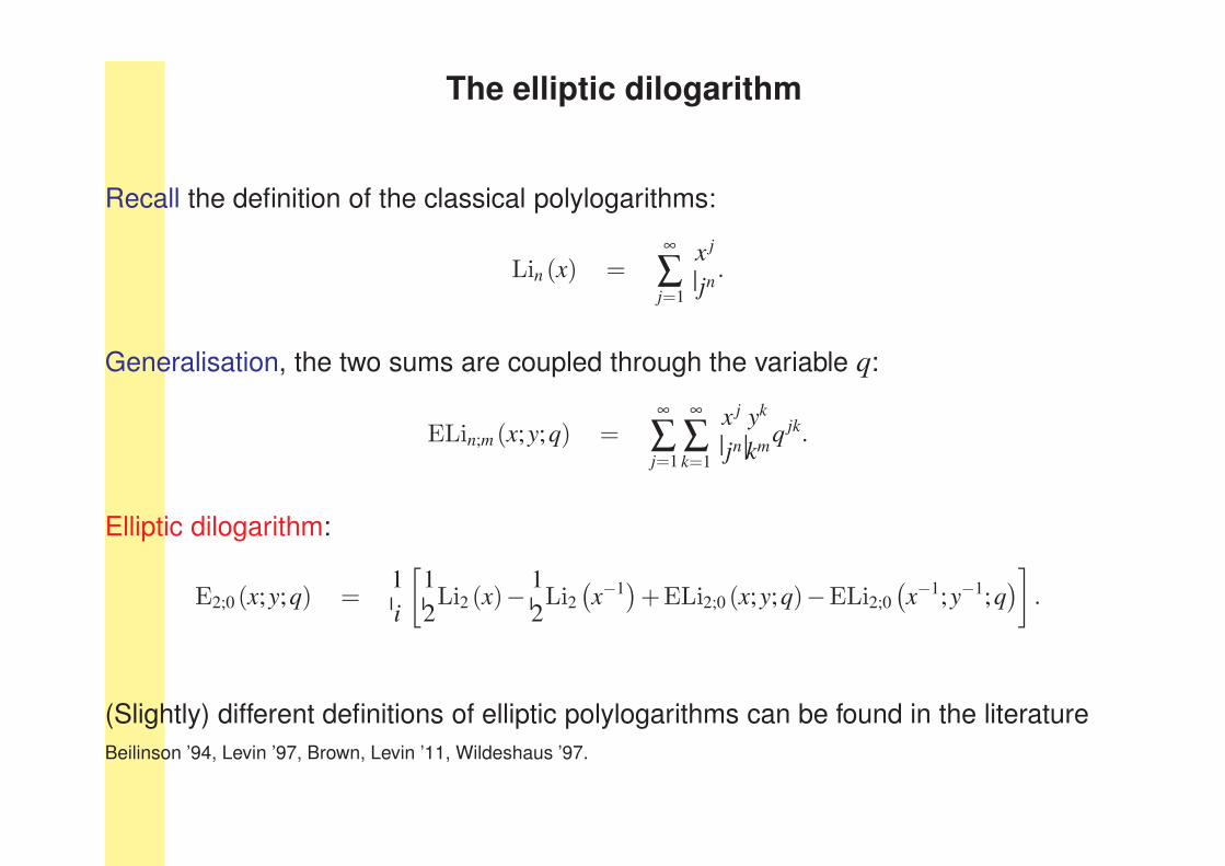
The elliptic dilogarithm
Recall the definition of the classical polylogarithms:
Lin (x) =∞
∑j=1
x j
jn.
Generalisation, the two sums are coupled through the variable q:
ELin;m (x;y;q) =∞
∑j=1
∞
∑k=1
x j
jn
yk
kmq jk.
Elliptic dilogarithm:
E2;0 (x;y;q) =1
i
[1
2Li2 (x)−
1
2Li2(x−1)+ELi2;0 (x;y;q)−ELi2;0
(x−1;y−1;q
)]
.
(Slightly) different definitions of elliptic polylogarithms can be found in the literature
Beilinson ’94, Levin ’97, Brown, Levin ’11, Wildeshaus ’97.

Elliptic curves again
The nome q is given by
q = eiπτ with τ =ψ2
ψ1
= iK(k′)
K(k).
Elliptic curve represented by
x1
x2
x3
X
Algebraic variety
F = 0
x
y
Weierstrass normal form
y2 = 4x3 −g2x−g3
Re z
Im z
Torus
C/Λ
Re w
Im w
Jacobi uniformization
C∗/q2Z

The arguments of the elliptic dilogarithms
Elliptic curve: Cubic curve together with a choice of a rational point as the origin O.
Distinguished points are the points on the intersection of the cubic curve F = 0 with
the domain of integration σ:
P1 = [1 : 0 : 0] , P2 = [0 : 1 : 0] , P3 = [0 : 0 : 1] .
Choose one of these three points as origin and look at the image of the two other
points in the Jacobi uniformization C∗/q2Z of the elliptic curve. Repeat for the two
other choices of the origin. This defines
w1,w2,w3,w−11 ,w−1
2 ,w−13 .
In other words: w1,w2,w3,w−11 ,w−1
2 ,w−13 are the images of P1, P2, P3 under
Ei −→ WNF −→ C/Λ −→ C∗/q2Z.

The full result in terms of elliptic dilogarithms
The result for the two-loop sunset integral in two space-time dimensions with arbitrary
masses:
S =4
[(t −µ2
1
)(t −µ2
2
)(t −µ2
3
)(t −µ2
4
)]14
︸ ︷︷ ︸
algebraic prefactor
K (k)
π
︸ ︷︷ ︸
elliptic integral
3
∑j=1
E2;0 (w j;−1;−q)
︸ ︷︷ ︸
elliptic dilogarithms
t momentum squared
µ1,µ2,µ3 pseudo-thresholds
µ4 threshold
K(k) complete elliptic integrals of the first kind
k,q modulus and nome
w1,w2,w3 points in the Jacobi uniformization
The two-loop sunset integral around four dimensions
The result in D = 4−2ε dimensions
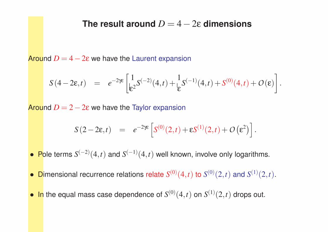
The result around D = 4−2ε dimensions
Around D = 4−2ε we have the Laurent expansion
S (4−2ε, t) = e−2γε
[1
ε2S(−2)(4, t)+
1
εS(−1)(4, t)+S(0)(4, t)+O (ε)
]
.
Around D = 2−2ε we have the Taylor expansion
S (2−2ε, t) = e−2γε[
S(0)(2, t)+ εS(1)(2, t)+O(ε2)]
.
• Pole terms S(−2)(4, t) and S(−1)(4, t) well known, involve only logarithms.
• Dimensional recurrence relations relate S(0)(4, t) to S(0)(2, t) and S(1)(2, t).
• In the equal mass case dependence of S(0)(4, t) on S(1)(2, t) drops out.

Generalisations of the Clausen and Glaisher functions
The Clausen and Glaisher functions are defined by (x = eiϕ):
Cln(ϕ) =
12i
[Lin (x)−Lin
(x−1)],
12
[Lin (x)+Lin
(x−1)],
Gln(ϕ) =
12
[Lin (x)+Lin
(x−1)], n even,
12i
[Lin (x)−Lin
(x−1)], n odd.
Elliptic generalisation:
En;m (x;y;q) =
=
1i
[12Lin (x)− 1
2Lin(x−1)+ELin;m (x;y;q)−ELin;m
(x−1;y−1;q
)], n+m even,
12Lin (x)+
12Lin(x−1)+ELin;m (x;y;q)+ELin;m
(x−1;y−1;q
), n+m odd.

The multi-variable case
In S(1)(2, t) we encounter one multi-variable function.
Sum representation:
E0,1;−2,0;4 (x1,x2;y1,y2;q) =
1
i
{[ELi2;0 (x1;y1;q)−ELi2;0
(x−1
1 ;y−11 ;q
)]×
1
2
[Li1 (x2)+Li1
(x−1
2
)]
+∞
∑j1=1
∞
∑k1=1
∞
∑j2=1
∞
∑k2=1
k21
j2 ( j1k1 + j2k2)2
(
xj11 y
k11 − x
− j11 y
−k11
)(
xj22 y
k22 + x
− j22 y
−k22
)
q j1k1+ j2k2
}
Integral representation:
E0,1;−2,0;4 (x1,x2;y1,y2;q) =
q∫
0
dq1
q1
q1∫
0
dq2
q2
[E0;−2 (x1;y1;q2)−E0;−2 (x1;y1;0)]E1;0 (x2;y2;q2)

The alphabet
All arguments for the x’s and y’s are from the set
{w1,w2,w3,w
−11 ,w−1
2 ,w−13 ,1,−1
}.

The ε1-term S(1)(2, t) of the expansion around D = 2−2ε
Recall: At O(ε0) we had
S(0)(2, t) =ψ1
π
3
∑j=1
E2;0 (w j;−1;−q)
At O(ε1) we have now
S(1)(2, t) =ψ1
π
[3
∑j=1
E3;1 (w j;−1;−q) + weight 3 terms
]
with
E3;1 (x;y;q) =1
i
[1
2Li3 (x)−
1
2Li3(x−1)+ELi3;1 (x;y;q)−ELi3;1
(x−1;y−1;q
)]
.
Remark: ELi3;1 is of weight 4.

The full result for S(1)(2, t)
If you are really curious:
S(1)(2,t) =ψ1
π
{[
−2
3
3
∑j=1
ln
(
m2j
µ2
)
−6E1,0 (−1;1;−q)+3
∑j=1
(
E1;0
(w j;1;−q
)−
1
3E1;0
(w j;−1;−q
))]
3
∑k=1
E2;0 (wk;−1;−q)
−23
∑j=1
1
2i
{
Li2,1(w j,1
)−Li2,1
(
w−1j ,1
)
+Li3(w j
)−Li3
(
w−1j
)
+3ln(2)[
Li2(w j
)−Li2
(
w−1j
)]}
+3
∑j=1
[4E0,1;−2,0;4
(w j,w j;−1,−1;−q
)−6E0,1;−2,0;4
(w j,w j;1,−1;−q
)+6E0,1;−2,0;4
(w j,−1;−1,1;−q
)]
+3
∑j1=1
3
∑j2=1
[2E0,1;−2,0;4
(w j1,w j2;1,−1;−q
)−E0,1;−2,0;4
(w j1,w j2;−1,−1;−q
)−E0,1;−2,0;4
(w j1,w j2;−1,1;−q
)]
+3
∑j=1
E3;1
(w j;−1;−q
)
}

Conclusions
Question: What is the next level of sophistication beyond multiple polylogarithms for
Feynman integrals?
Answer: Elliptic stuff.
• Algebraic prefactors as before.
• Elliptic integrals generalise the period π.
• Elliptic (multiple) polylogarithms generalise the (multiple) polylogarithms.
• Arguments of the elliptic polylogarithms are points in the Jacobi uniformization of
the elliptic curve.
• Weight may raise by two units in the ε-expansion.

![Feynman integrals and multiple polylogarithms arXiv:0705.0900v1 … · arXiv:0705.0900v1 [hep-ph] 7 May 2007 MZ-TH/07-06 Feynman integrals and multiple polylogarithms Stefan Weinzierl](https://static.fdocuments.us/doc/165x107/60546717048db466a451dca9/feynman-integrals-and-multiple-polylogarithms-arxiv07050900v1-arxiv07050900v1.jpg)