A Vision-based Navigation System of Mobile Tracking Robot

Jie Wu, Vac1av Snasel Dept. Computer Science, FEECS

VSB - Technical University of Ostrava

Ostrava, Czech Republic

defermat2008 @hotmail.com, vaclav. snasel @vsb.cz

Abstract-Based on the study of developments in many fields of computer vision, a novel computer vision navigation system for mobile tracking robot is presented. Three irrelevant technologies, pattern recognition, binocular vision and motion estimation, make up of the basic technologies of our robot. The non· negative matrix factorization (NMF) algorithm is applied to detect the target. The application method of NMF in our robot is demonstrated. Interesting observations on distance measurement and motion capture are discussed in detail. The reasons resulting in error of distance measurement are analyzed. According to the models and formulas of distance measurement error, the error type could be found, which is helpful to decrease the distance error. Based on the diamond search (DS) technology applied in MPEG· 4, an improved DS algorithm is developed to meet the special requirement of mobile tracking robot.

Index Terms-mobile robot, navigation, computer vision, non· negative matrix factorization, binocular vision, motion estimation.

I. INTRODUCTION

A main aim of robotics research is to gain knowledge about

the nature of intelligence, to make computers more useful to

human. Creating more intelligent computers will make robots

more useful to people. Mobile tracking robot can offer some

attractive home services closely related to our life. It will be

the most useful partner in our life in future. In our project, we

try to develop a kind of mass producible, low-cost autonomous

mobile tracking robot.

Indubitably, vision navigation system is one of the most

important systems in mobile robot. Computer vision for mobile

robot navigation became a hot subject since the end of 1970s.

It has achieved great progress in the field of computer vision

in recent several decades. Many interesting technologies were

applied in this field continuously. Most research work on

mobile robot vision navigation is focused on map building,

self-localization, path planning, and obstacle avoidance.

G. N. DeSouza et al. [1] investigated the developments of

twenty years in the field of vision for mobile robot navigation.

The developments can be divided into indoor navigation and

outdoor navigation.

For the indoor navigation, it includes three broad groups:

map-based, map-building-based and mapless navigation. Map­

based navigation systems depend on user-created geometric

models or topological maps of the environment. Map-building­

based navigation systems use sensors to construct their own

978-1-4244-6588-0/10/$25.00 ©2010 IEEE

Ajith Abraham Machine Intelligence Research Labs, MIR Labs

http://www.mirlabs.org

Washington, USA

ajith.abraham@ieee.org

geometric or topological models of the environment and then

use these models for navigation. Mapless navigation systems

use no explicit representation at all about the space in which

navigation is to take place, but other resort to recognize

objects found in the environment or to track those objects by

generating motions based on visual observations. The problem

of robotic mapping is that of acquiring a spatial model of

a robot's environment. It is a process for robot to perceive

the outside world. Sebastian Thrun [2] surveyed major algo­

rithms of robotic mapping, including Kalman filter techniques,

approaches based on Dempster's expectation maximization

algorithm, occupancy grid techniques, and so on.

For the outdoor navigation, which usually involves obstacle­

avoidance, land-mark detection, map-building or updating, and

position estimation, it can be divided into structured and

unstructured environments according to the level of structure of

the environment. In general, outdoor navigation in structured

environments requires some sort of road-following; while out­

door navigation in unstructured environments, which doesn't

require regular properties used to be perceived or tracked for

navigation, can make use of at most a generic characterization

of the possible obstacles in the environment.

Each sort of those methods mentioned above has its own

technical characteristics. The central computations involved

in map-based navigation can be divided into four steps: ac­

quire sensory information, detect landmarks, establish matches

between observation and expectation and calculate position.

The map-building-based approaches try to explore the en­

vironment and build an internal representation of it for the

robot, such as 3D coordinates, occupancy grid or metric­

topological representation, etc. Mapless navigation does not

need map, in which the robot motions are determined by

observing and extracting relevant information of environment

such as walls, desks, doorways, etc. Optical flow-based and

appearance-based are two prominent techniques used in maples

navigation. Outdoor navigation is often executed by cars or

wheeled vehicles. The road-following for outdoor navigation

in structured environments means an ability to recognize the

lines that separate the lanes or separate the road from the berm,

the texture of the road surface, and the adjoining surfaces, etc.

In unstructured outdoor navigation, those techniques include

external camera observation, far-point landmark triangulation,

3053

global positioning, etc.

Human eyes and vision navigation system take on similar

fundamentality in human and mobile robot, respectively. From

the perspective of bionics, the researches on human eyes

are referential and significant to the development of robotic

vision system. With the important functions, such as binocular

parallax, motion parallax, accommodation and convergence,

human eyes can extract depth cue out of scene, which finally

results in the ability of depth perception. Similarly, if the

robotic vision system performs similar functions to those of

human eyes, the robot will be more intelligent.

By analyzing those functions of human eyes more carefully,

it can be found that there are three processes which are primary

and essential to robot: target recognition, distance estimation

and motion capture. Target recognition, or object recognition,

can tell robot what the target is. Distance estimation can

describe the environment; tell robot where the target is and

where robot itself is, which actually means some certain kind

of stereo vision capability. Motion capture can tell robot how to

follow the target. Based on these three primary processes, the

mobile tracking robot can possess some important capabilities.

In this paper, we present an approach of computer vision

navigation for mobile tracking robot. We try to use cheap

cameras and simple algorithm to realize the functions needed

by mobile tracking robot. The main process is summarized as

follows.

Step 1: Target Recognition. The features of target are

abstracted from images taken by the vision system of the

mobile robot. In this step, the robot can perceive the target.

Step 2: Distance Estimation. According to the images taken

by eyes of the mobile robot vision system, the distance of target

can be gotten depending on vision measurement technology.

Of course, if the map is necessary for the robot to select its

route or avoid obstacle, the robot can redraw the scene as a

map. Therefore, the robot can know the position of target and

get the environment information in this step.

Step 3: Motion Capture. When the target is moving, the

robot can compute the motion vector of target using search

algorithm. According to the target motion vector, the robot

can control its drive system to follow the target. Therefore,

the robot can know how to track the target.

The rest of this paper is organized as follows. Section 2

discusses the application of non-negative matrix factorization

in robot navigation. The data processing and an example are

demonstrated in this section. Section 3 and section 4 analyze

the distance estimation and the motion estimation, respectively.

Section 5 gives a model to validate the approach presented in

this paper, concludes the works of this paper, also discusses

some future work.

II. TARGET RECOGNITION

In this step, the essence of target recognition is the mecha­

nism of computer to cognise object. Undoubtedly, the research

on mechanism of the human brain to perceive the world is

helpful to resolve our problem.

Some researchers found psychological and physiological

evidence for parts-based representations in the brain. Conse­

quently, certain computational theories of object recognition

were presented based on such representations. According to

the parts-based representations, the objects can be represented

as

Objecti

where

bil x Parh + bi2 x Part2 + ...

+bij x Partj + ...

if part j is present in object i if part j is absent from object i.

Similarly, the object of image can be represented as

bil x Featurel + bi2 x Feature2 + ...

+bij x Featurej + ...

where bij ::::: 0 are the participation weight of feature j in

image i. Because each pixel is represented by its light intensity

measured by a non-negative value, the participation weight bij is inevitably a non-negative number.

The parts-based representations offer an approach to recon­

struct or recognize the world. Object can be cognised based on

parts perceived by human brain, and image can be recognized

based on features abstracted by computer. Consequently, the

hard core of our problem becomes to find a method by which

computer abstracts features, or parts, from images.

D. D. Lee and H. S. Seung [3] demonstrated an algorithm

for non-negative matrix factorization (NMF) that could learn

parts of objects, such as parts of faces and semantic features

of text. In their opinion, the image database is regarded as an

nxm matrix V, each column of which contains n non-negative

pixel values of one of the m facial images. Then the NMF

construct approximate factorizations of the form V � W H, or

r

ViI' = (WH)il' = L WiaHal' a=l

The r columns of Ware called basis images. Each column of

H is called an encoding and is in one-to-one correspondence

with a face in V. An encoding consists of the coefficients by

which a face is represented with a linear combination of basis

images. The dimensions of the matrix factors Wand H are

n x rand r x m, respectively. The rank r of the factorization

is generally chosen so that (n+m) x r < nm, and the product

W H can be regarded as a compressed form of the data in V. To find an approximate factorization V � W H, cost

function shall be defined firstly, which quantify the quality

of the approximate. Euclidean distance and Kullback-Leibler

divergence, or relative entropy, are two useful measures. The

cost functions based on them can be expressed as follows,

respectively.

IIV - WHI12 = L [Vij - (WH)ij]

2

ij

3054

D(vIIWH) = 2:: [VijlOg (:;)ij - Vij + (WH)ij ]

'J

The Euclidean distance II V -W HII is non-increasing under

the update rules

(WTV)a/-L Ha/-L r- Ha/-L (WTW H)a/-L

(VHT)ia Wia r- Wia

(W H HT)ia

The divergence D(VIIW H) is non-increasing under the

update rules

The Euclidean distance and divergence are invariant under

these respective updates if and only if Wand H are at a

stationary point of the distance or divergence, respectively.

D. D. Lee and H. S. Seung also gave two examples of

NMF application on facial images and semantic analysis. In

the facial image application, the grey intensities of each image

are first linearly scaled so that the pixel mean and standard

deviation equal 0.25, and then clip to the range [0, 1]. NMF is

performed with the iterative algorithm, starting with random

initial conditions for W and H. The algorithm converges

usually in 50 iterations in their example. In fact, they have

proved the convergence [4] of the NMF update rules.

According to the algorithm and application on facial im­

ages, it is obvious that the NMF can be applied to recognize the

object in our problem, no matter it is face, back or something

else. Because the NMF has the ability to learn the parts-based

features of object, the robot can recognize target if only it has

this kind of ability.

A feasible process of target recognition for our mobile

tracking robot may be is

Step 1: The robot captures the image of target multi­

angularly, such as from head to toe, from the front to the back,

from far to near, etc.

Step 2: Linear scale all these images. Construct matrix V by converting each image to a column vector and combining

them.

Step 3: Process the matrix V by implementing NMF algo­

rithm, and then get the basis images Wand encoding matrix

H. Step 4: For a new image matrix U that includes the parts of

target features or some columns of matrix W, new encoding

matrix J can be extracted by W-1U.

Step 5: Find the part in matrix J that is with the shortest

distance to another part in matrix H. This part in Matrix J contains the position information of target in matrix U. It

means we have found the target in the new image.

Fig. 1 shows briefly the main procedure of data processing.

Firstly, the color images are converted to grey images, see

(a)

(b)

Fig. I. Data processing by using NMF. (a) hand-aligned grey images, each of them corresponds to a column of matrix V; (b) the parts-based images corresponding to basis matrix W.

Fig. lea). To facilitate comparison with the matrix V, the nine

frontal views are aligned by hand, each of them corresponds

to a column of matrix V. Fig. I(b) shows the parts-based faces

transformed by the basis image matrix W.

In the NMF algorithm, the rank r is an important parameter

that decides the dimension of characteristic subspace. The

determining of r shall be helpful to reduce the dimension of

image matrix, but also to express target features effectively.

However, there is no good way to determine it nowadays.

In [5], N.D. Ho indicated that the problem of determining

the non-negative rank can be solved in finite time by looping

through r = 1, 2, ... , min(n, m) because the upper bound of

the non-negative rank is min(n, m). Additionally, N.D. Ho et al. [6] compared the convergence speed of different algorithms,

which can be a reference to the determining of r value.

III. MEASURE OF DISTANCE

Binocular stereo triangulation, see Fig. 2(a), is a simple and

effective approach in computational stereo [7]. It also can be

regarded as a special case of two-view geometry [8]. Given

the distance between aperture diaphragm OL and OR, called

baseline B, and the focal length f of the cameras, object

distance D may be computed by similar triangles as

D = fB

= K� Xl + Xr npixel

(I)

where Xl and Xr are the absolute horizontal distance between

image point and the left and right image center respectively, K is constant, npixel is displacement of pixels. Indeed binocular

stereo triangulation is outdated. But if used appropriately, it

will be very effective.

According to (1), the maximum estimated object distance

depends on maximum focal length f, baseline B and minimum

pixel displacement npixel. Obviously, the maximum value is

Dmax = K fmaxBmax, where Dmax, fmax and Bmax are maximum value of D, f and B, respectively.

It should be noticed that the lens model in Fig. 2(a) is

pinhole model. The image of the object on the image plane

is top-bottom inverted and left-right inverted. And camera can

revise these inversions in real picture automatically. Finally,

the point on image plane lying at lower left corner may lie

at upper right corner in the real picture. Therefore, these

automatic revisions should be considered in measuring the

distance between image point and image center in the real

picture.

3055

• object

�o, D I !OL

� � f 'I i\

I ... Xl �! ... B II X,. .. I'"

(a)

'''' \'�

\0, �

iOR � i\ Xl �

(b)

• I I I I

OL � OR �

I Xl I - I Xr -----+-1-j4---

(c)

Fig. 2. Three cases of object position in image plane: the object lies (a) between two centers, (b) at the left of the left camera center, and (c) at the right of the right camera center.

As shown in Fig. 2(b) and (c), if the object lies at the left

of left camera or right of right camera, the object distance D may be computed respectively as

D = fB (2)

xr - Xl

D = fB (3)

Xl - Xr

In our experiment, we select two pan-tilt-zoom webcams as

the cameras of the mobile robot vision navigation system. The

webcams are very cheap. In practice, it is difficult to build

ideal binocular stereo system with nonverged geometry. For

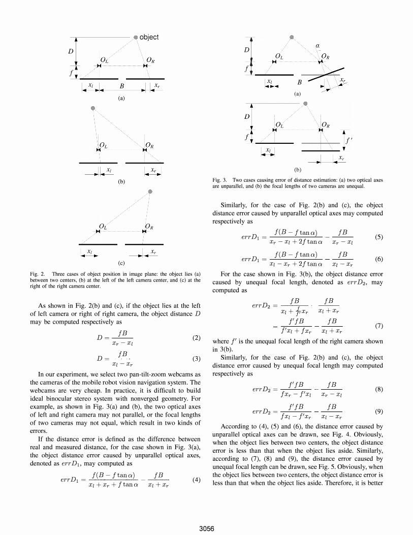
example, as shown in Fig. 3(a) and (b), the two optical axes

of left and right camera may not parallel, or the focal lengths

of two cameras may not equal, which result in two kinds of

errors.

If the distance error is defined as the difference between

real and measured distance, for the case shown in Fig. 3(a),

the object distance error caused by unparallel optical axes,

denoted as err D1, may computed as

errD1 = f(B - ftano:) _ fB (4)

Xl + Xr + f tan 0: Xl + Xr

a �

a. / ""--: OL lOR � �

!:�! ... B (a)

f •

OL OR � �

I I Xl I � �! I X,. ,'" (b)

Fig. 3. Two cases causing error of distance estimation: (a) two optical axes are unparal\el, and (b) the focal lengths of two cameras are unequal.

Similarly, for the case of Fig. 2(b) and (c), the object

distance error caused by unparallel optical axes may computed

respectively as

f(B - ftano:) fB errD1 = - (5)

Xr - Xl + 2ftano: Xr - Xl

f(B - f tan 0:) fB errD1 = (6)

Xl - Xr + 2f tan 0: xl -xr For the case shown in Fig. 3(b), the object distance error

caused by unequal focal length, denoted as err D2, may

computed as

errD2 = fB fB Xl + fXr Xl +Xr

f'fB fB (7) f'Xl + fXr Xl +Xr

where l' is the unequal focal length of the right camera shown

in 3(b).

Similarly, for the case of Fig. 2(b) and (c), the object

distance error caused by unequal focal length may computed

respectively as

f'fB fB errD2 = f f Xr - 'Xl Xr - Xl

f'fB fB errD2 = f f Xl - 'Xr Xl - Xr

(8)

(9)

According to (4), (5) and (6), the distance error caused by

unparallel optical axes can be drawn, see Fig. 4. Obviously,

when the object lies between two centers, the object distance

error is less than that when the object lies aside. Similarly,

according to (7), (8) and (9), the distance error caused by

unequal focal length can be drawn, see Fig. 5. Obviously, when

the object lies between two centers, the object distance error is

less than that when the object lies aside. Therefore, it is better

3056

O r-----------------------� � --- -- �,---,:-

,.--- -- - , ---- - -- - ' �

-0.1 V " , ,' -; '

- � , ,--E " .2- /'

e Qi

E .2-'-e Qi

a = 5° / a = 10° -0.2

V a = 15° a = 20°

-0.3 40 60 80 100

pixel displacement

(a) corresponding error of Fig. \ (a)

0 .---------------------.

�-------

�'-:::

"--

�

--" -'0.1 / ,,- ' - '

-� -

V " � ,.. J" / ...

, , , / a = 5° , -0.2

, a = 10° / a = 15°

If a = 20° -0 . 3

40 60 80 100

pixel displacement

(b) corresponding error of Fig. \ (b) and (c)

Fig. 4. The object distance error caused by unparallel optical axes. Baseline is 8 cm, and reference focal length is 4 cm.

to measure the object distance while the object lies between

two centers.

Based on the error analysis above, the unparallel optical

axis and unequal focal length can be corrected. Fig. 6 shows

the distance curves at different baseline after correction.

Equation (1) shows that the estimation range of distance is

directly proportional to f and B. If the robot wants to adjust

the distance range, it just need to increase or decrease focal

length f or baseline B. It is an effective way for the robot to

observe the object at very far or very close distance. But the

increase of f or B may also increase the object distance error,

which is a matter of course, because the further the object, the

larger the distance error.

IV. MOTION CAP TURE

If the robot can compute the object's motion vector from

every frame taken by its eyes, it can know the object motion,

and then can track it. An effective and popular method, called

block-matching motion estimation, has been widely applied

in various video coding standards, such as H.261, H.263,

MPEG-l, MPEG-2 and MPEG-4, and in motion-compensated

video coding technique. Many fast block-matching algorithms

have been developed, for example, 2-D logarithmic search,

three-step search, conjugate direction search, cross search, new

three-step search, four-step search, block-based gradient de­

scent search, etc. These fast block-matching algorithms exploit

different search patterns and search strategies for finding the

E .2-'-e Qi

E .2-e Qi

, 0 . 3 ,

, /'= 5 em ,

0 .2 /'= 6 em

, , 0.1 ' - .

o 20 40 60 80 100 120

0 . 8

0 . 6

0 . 4

0.2

0

pixel displacement

(a) corresponding error of Fig. \(a)

, , , ,

20 40

/'= 5 em /'= 6 em

60 80

pixel displacement

(b) corresponding error of Fig. \ (b) and (c)

Fig. 5. The object distance error caused by unequal focal length. Baseline is 8 cm, and reference focal length is 4 cm.

150 E .2-Q) 100 (J C ro (j)

'6 50

0 0

--- B=8em , \ - - - - B = 16 em ,

, , - -

\... ... ....... ...

B= 24 em

\S ...... -... ... .. -...... ....... - --

200 400 pixel displacement

Fig. 6. The distance curves at different baseline after correcting the errors.

optimum motion vector with drastically reduced number of

search points as compared with the full search algorithm that

test all the candidate blocks within the search window.

Shan Zhu and Kai Kuang Ma proposed a simple, robust

and efficient fast block-matching motion estimation algorithm,

called diamond search (DS) [9]. The DS algorithm employs

two search patterns, called large diamond search pattern

(LDSP) and small diamond search pattern (SDSP). We applied

the DS algorithm to compute the object's motion vector in our

experiment.

In contrast, it is necessary to repeat briefly the DS algorithm

firstly. After discussing it in detail, the improved DS algorithm

used in mobile tracking robot will be introduced.

The DS algorithm is summarized as follows, as shown in

3057

-7 -6 -5 -4 -3 -2 -1 0 1 2 3 4 5 6 7 -7 -6 -5 -4 • -3

� -2 · N· -1 . is • 0 . � • 1 • • • 2 • • 3 4 5 6 7

Fig. 7. Search path example which leads to the motion vector (-4, -2) in five search steps-four times of LDSP and one time SDSP at the final step. There are 24 search points in total-taking nine, five, three, three, and four search points at each step, sequentially.

-7 -6 -5 -4 -3 -2 -1 0 1 2 3 4 5 6 7 -7 -6 -5 -4 -3 -2 0 • -1 06. ••• 0 06. •••••

06. • •• 2 0 • 3 4 5 6 7

Fig. 8. Search path example which leads to the motion vector (-2, 0) in three search steps: once combination of LDSP and SDSP, once LDSP and once SDSP at the last step. There are 21 search points in total: taking thirteen, five and three search points at each step, sequentially.

Fig. 7.

Step 1: The initial LDSP is centered at the origin of the

search window, and the 9 checking points of LDSP are tested.

If the minimum block distortion (MBD) point calculated is

located at the center position, go to Step 3; otherwise, go to

Step 2.

Step 2: The MBD point found in the previous search step

is re-positioned as the center point to form a new LDSP. If the

new MBD point obtained is located at the center position, go

to Step 3; otherwise, recursively repeat this step.

Step 3: Switch the search pattern from LDSP to SDSP. The

MBD point found in this step is the final solution of the motion

vector which points to the best matching block.

Firstly, the DS algorithm computes every block's motion

vector; however, for mobile robot, it just need to only compute

the motion vector of interested one rather than every block.

Secondly, the DS algorithm has perfect performance if the

object moves to one of the 9 positions at LDSP in next frame;

(a) the reference frame

(b) the matched frame to compute motion vector

Fig. 9. Two frames of a video. (a) is the reference frame, and (b) is the next frame. The motion vector is computed according to these adjacent frames. The black square is target. The circle one is disturbing object. Both of them are moved.

but if the object moves outside of LDSP or to one of the

five positions at SDSP in next frame, it cannot find the object

any more. Considering what the robot track is human, general

movement is forward or backward, and rarely very fast left or

right, so the moving outside of LDSP in next frame could be

neglected. At the same time, the initial search should include

LDSP and SDSP.

In our experiment, we found that the block size has impor­

tant effect to the search result. The perfect situation is that the

search block has the same size to the object in image. If the

block is greater than the object, search is not very good.

Based on the discussion above, the improved DS algorithm

could be summarized as follows, as shown in Fig. 8.

Step 1: According on the object feature, set the block size

equals to the object size. The initial search including LDSP

and SDSP is centered at the origin of the search window, and

the 13 checking points are tested. If the MBD point calculated

is located at the center position, go to Step 3; otherwise, go

to Step 2.

Step 2: The MBD point found in the previous search step

is re-positioned as the center point to form a new LDSP. If the

new MBD point obtained is located at the center position, go

to Step 3; otherwise, recursively repeat this step.

Step 3: Switch the search pattern from LDSP to SDSP. The

MBD point found in this step is the final solution of the motion

vector which points to the best matching block.

Fig. 9(a) and (b) are two frames of a video. It shows

the movement of a circle and a square object. In fact, the

square one is the target, the method presented in this paper can

estimate the object's distance and compute its motion vector,

see Fig. 10.

3058

100 a; .[ 200 !ii u .� 300 >

400

o 100 200 300 400 500 600 horizontal pixel

Fig. 10. The motion vector of square target. The upper left comer is the origin of image. The vector means motion vector that shows the target's displacement from start to end point.

V. CONCLUSION

An ease way to validate the approach of vision-based

navigation system discussed in this paper is to connect we­

bcams with computer. After receiving data from webcams and

calculating the target's distance and motion vector, computer

send control parameters to robot. LEGO Mindstorms NXT is a

good choice for the robot. It's not necessary to fix the webcams

on LEGO robot in this verification model. The final purpose

of this model is to control the left and right wheel of LEGO

robot rotate correctly according to the movement of target.

Fig. 11 shows the flow of the verification model. The

webcams capture frames and send these data to computer,

computer then recognizes target and calculates its distance and

motion vector to control robot's speed and direction so as to

follow the target.

In sum, the vision-based system of computer vision nav­

igation for mobile tracking robot mentioned in this paper

consists of three main parts called target recognition, distance

measurement and motion capture, respectively.

The NMF algorithm is applied in recognition part to per­

ceive target. Because NMF is a parts-based algorithm, it can

recognize the target after learning the parts-based features.

The NMF is an important development of the research on

perception, which provides a feasible approach for machine

to simulate the cognitive methods in human brain. However,

NMF is not a perfect algorithm. For example, its localization

performance of basis image is not satisfied; when it finds

projecting basis vector to compress high dimensional data

to low dimensional data, it ignores an important information

that original data samples belong to different categories; also,

there is no clear requirements of statistical relationship of the

data after dimension reduction. Accordingly, many improved

algorithms were developed, such as local non-negative matrix

factorization (LNMF) [10], [11], sparseness non-negative ma­

trix factorization [12], [13], [14], fisher non-negative matrix

factorization (FNMF) [15], etc. It's necessary to optimize the

NMF according to the requirements of mobile tracking robot;

to find a method to determine the optimized rank r; to simplify

the recognition steps.

The reasons resulting in object distance error and its cor­

rection methods are discussed in detail. When the object lies

between two optical axes, the distance error is less than that

q Computer

I Object Recognition I LEGO NXT

Fig. II. The How of the verification model.

when object lies aside. An improved DS algorithm is developed

to meet the special requirement of mobile tracking robot. In

future, the distance estimation model should be developed. It

will be very good for the robot if it can fitting the distance

curves at different focal length f and baseline B easily.

Additionally, simpler and faster search algorithm should be

developed. Of course, all of these should be realized by cheap

hardware.

REFERENCES

[I] G. N. DeSouza and A. C. Kak, "Vision for mobile robot navigation: a survey," IEEE Trans. Pattern Analysis and Machine Intelligence, vol. 24, no. 2, pp. 237-267, Feb. 2002.

[2] S. Thrun, "Robotic mapping: a survey," School of Computer Science, Carnegie Mellon University, Pittsburgh, Tech. Rep., Feb. 2002.

[3] D. D. Lee and H. S. Seung, "Learning the parts of objects by non­negative matrix factorization," Nature, vol. 401, pp. 788-791, Oct. 1999.

[4] S. Se, D. G. Lowe, and 1. J. Little, "Vision-based global localization and mapping for mobile robots," IEEE Trans. on Robotics, vol. 21, no. 3, pp. 364--375, Jun. 2005.

[5] N.-D. Ho, "Non-negative matrix factorization algorithms and applica­tions," Ph.D. dissertation, UNIVERSIT07 CATHOLIQUE DE LOU­VAIN, Jun. 2008.

[6] N.-D. Ho, P. V. Dooren, and V. D. Blondel, "Descent methods for non­negative matrix factorization," in Numerical Linear Algebra in Signals, Systems and Control, Aug. 2009, ch. I.

[7] M. Z. Brown, D. Burschka, and G. D. Hager, "Advances in computational stereo," IEEE Trans. on Pattern Analysis and Machine Intelligence, vol. 25, no. 8, pp. 993-1008, 2003.

[8] R. Hartley and A. Zisserman, Multiple View Geometry in Computer Vision. UK: Cambridge University Press, 2003.

[9] S. Zhu and K. K. Ma, "A new diamond search algorithm for fast block­matching motion estimation," IEEE Trans. on Image Procesing, vol. 9, no. 2, pp. 287-290, Feb. 2000.

[10] S. Z. Li, X. Hou, H. Zhang, and Q. Cheng, "Learning spatially localized, parts-based representation," in Proc. of the 2001 IEEE Computer Society Con! on Computer Vision and Pattern Recognition, vol. 1, 2001, pp. 207-212.

[I I] T. Feng, S. Z. Li, H.-Y. Shum, and H. Zhang, "Local non-negative matrix factorization as a visual representation," in Proc. of the 2nd International Con! on Development and Learning, Jun. 2002, pp. 178-183.

[12] W. Liu, N. Zheng, and X. Lu, "Non-negative matrix factorization for visual coding," in Proc. IEEE International Con! on Acoustics, Speech, and Signal Processing, vol. 3, Apr. 2003, pp. 293-296.

[I3] P. O. Hoyer, "Non-negative sparse coding," in Proc. Neural Networks for Signal Processing, Nov. 2002, pp. 557-565.

[14] --, "Non-negative matrix factorization with sparseness constraints," Journal of Machine Learning Research, pp. 1457-1469, May 2004.

[15] Y. Wang, Y. Jia, C. Hu, and M. Turk, "Fisher non-negative matrix fac­torization for learning local features," in Asian Conference on Computer Vision, 2004.

3059