A very minimal introduction to TikZ∗

Jacques CremerToulouse School of Economics

jacques.cremer@tse-fr.eu

March 11, 2011

Contents

1 Introduction 3

2 Setting up a picture 3

3 Drawing lines and curves 43.1 Simple straight lines . . . . . . . . . . . . . . . . . . . . . . . . . 43.2 Scaling pictures . . . . . . . . . . . . . . . . . . . . . . . . . . . . 53.3 Arrows and the like . . . . . . . . . . . . . . . . . . . . . . . . . . 63.4 Changing the thickness of lines . . . . . . . . . . . . . . . . . . . 73.5 Dashes and dots . . . . . . . . . . . . . . . . . . . . . . . . . . . 83.6 Colors . . . . . . . . . . . . . . . . . . . . . . . . . . . . . . . . . 83.7 Pictures in the middle of the text . . . . . . . . . . . . . . . . . . 83.8 Curves . . . . . . . . . . . . . . . . . . . . . . . . . . . . . . . . . 83.9 Plotting functions . . . . . . . . . . . . . . . . . . . . . . . . . . 11

4 Filling up areas 124.1 Filling up simple areas . . . . . . . . . . . . . . . . . . . . . . . . 124.2 Filling up arbitrary areas . . . . . . . . . . . . . . . . . . . . . . 13

5 Putting labels in pictures 13

6 Integration with Beamer 16

7 Hints and tricks 17

∗Thanks to Christophe Bontemps, Michel-Benoıt Bouissou and Florian Schuett for com-ments which have improved this document.

1

8 Examples 178.1 Hotelling . . . . . . . . . . . . . . . . . . . . . . . . . . . . . . . . 17

8.1.1 The whole picture . . . . . . . . . . . . . . . . . . . . . . 178.1.2 Step by step . . . . . . . . . . . . . . . . . . . . . . . . . 18

8.2 Vertical differentiation . . . . . . . . . . . . . . . . . . . . . . . . 188.2.1 The whole picture . . . . . . . . . . . . . . . . . . . . . . 188.2.2 Step by step . . . . . . . . . . . . . . . . . . . . . . . . . 18

8.3 A curve . . . . . . . . . . . . . . . . . . . . . . . . . . . . . . . . 198.3.1 The whole picture . . . . . . . . . . . . . . . . . . . . . . 198.3.2 Step by step . . . . . . . . . . . . . . . . . . . . . . . . . 20

8.4 Tangency . . . . . . . . . . . . . . . . . . . . . . . . . . . . . . . 208.4.1 The whole picture . . . . . . . . . . . . . . . . . . . . . . 208.4.2 Step by step . . . . . . . . . . . . . . . . . . . . . . . . . 21

8.5 Consumer surplus . . . . . . . . . . . . . . . . . . . . . . . . . . . 228.5.1 The whole picture . . . . . . . . . . . . . . . . . . . . . . 228.5.2 Step by step . . . . . . . . . . . . . . . . . . . . . . . . . 22

8.6 Plotting lots of curves . . . . . . . . . . . . . . . . . . . . . . . . 23

9 Conclusion 24

2

1 Introduction

The aim of this document is to provide the minimum useful introduction to theTikZ package (written by Till Tantau), which enables you to do nice figures inLATEX. I hope it will encourage for further exploration, but I also believe thatat least 70% of the figures found in the economic literature can be drawn withthe commands I present here.1

There are certainly mistakes left in this document. Be careful and if youfind a mistake, drop me an e-mail!

The latest version of this document can be found at http://bit.ly/gNfVn9.

2 Setting up a picture

Just write2 \usepackage{tikz} in the preamble of your document. ModernTEX engines3 such as MikTeX will automatically install the package. Thenwhen you want to do a picture just write\begin{tikzpicture}

code

\end{tikzpicture}

If you want to do a figure (you know the kind of thing that “floats” to the topof the page) you need to set it up as\begin{figure}

\begin{tikzpicture}

code

\end{tikzpicture}

\caption{Do not forget!

Make it explicit enough that readers

can figure out what you are doing.}

\end{figure}

You then compile your document using pdfTEX or XeTEX.

1There is another popular package for doing figures in LATEX, PSTricks, whose originalversion is due to the economist Tim van Zandt. The two packages are pretty much equivalentin terms of ease of use and features. TikZ has the advantage of better compatibility withpdfTEX; PSTricks has the advantage of some nice commands for drawing curves. You canfind an introduction to PSTricks in the book “The LATEX Graphics Companion”.

2This assumes that you are using LATEX. TikZ can also be used in raw TEX, but if youare hardcore enough to do that, you probably are better off going straight to the manual.

3I do not know how to set up TikZ for use with Scientific Word (which you should not beusing in any case). If you know how to do it, please tell me so that I can put the instructions inthe next version of this document. (I assume that if you can do it is still pretty uncomfortable,as the code for the pictures will be in the infamous gray boxes.)

3

There is a very extensive (over 700 pages!) manual. You can find it athttp://bit.ly/e3eQQd.4,5,6

3 Drawing lines and curves

3.1 Simple straight lines

To draw a line you do something like\begin{tikzpicture}

\draw (0,0) --(1,2);

\end{tikzpicture}

and you get

TikZ automatically draws a line between the points (0,0) and (1,2) and setsup the right space for the figure (by default, coordinates are in centimeters).You can do a sequence of segments which goes from point to point:\begin{tikzpicture}

\draw (0,0) --(1,2) -- (2,3) -- (1,0);

\end{tikzpicture}

to get

(I have added the grid lines on the graphic to make it clearer. This is donethrough the command \draw[help lines] (0,0) grid (2,3);, which draws agrid from (0,0) to (2,3). The “help lines” option makes the presentation neater

4You can also find it on your computer once TikZ is installed. Go to the command linewindow and type texdoc pgf and choose pgfmanual.pdf in the list which is offered. Or, ifyou are using the WinEdt editor, you you can go to LATEX help and ask it for the help of thepgf package. (See the manual about the reasons for the two names TikZ and pgf.)

5In French, there also exists an introduction to TikZ which is shorter (but still 189 pageslong) and may be more accessible than the manual. It is called “TikZ pour l’impatient”, waswritten by Gerard Tisseau and Jacques Duma, and can be found at http://math.et.info.

free.fr/TikZ/bdd/TikZ-Impatient.pdf.6There are a number of wysiwyg or semi-wysiwyg tools which can help you do graphics.

For instance, while still in beta state TikZEdt seems useful (http://code.google.com/p/tikzedt/).

4

— I discuss this below. I will add grid lines as useful in what follows withoutputting the corresponding line in the code.)

Of course, you can put several lines on the same graph:\begin{tikzpicture}

\draw (0,0) --(1,2) -- (2,3) -- (1,0);

\draw (3,0) -- (1.5,0.5);

\end{tikzpicture}

yields

Notice the semi-colons “;” at the end of lines — it is these semi-colons whichmark the end of instructions. You will see below examples where one instructionis spread over several lines. We could also put several instructions on one line:in the last picture I could have written\draw (0,0) --(1,2) -- (2,3) -- (1,0); \draw (3,0) -- (1.5,0.5);

without changing the output. You can also add and suppress spaces, for instancein order to make the code easier to read, without changing anything in theoutput.

3.2 Scaling pictures

One very useful feature of TikZ is that you can blow up the picture, by addingan option “scale” to the environment.\begin{tikzpicture}[scale=3]

\draw (0,0) -- (1,1);

\end{tikzpicture}

to get

which you can compare to the following:\begin{tikzpicture}

\draw (0,0) -- (1,1);

\end{tikzpicture}

5

which yields

You can scale only one dimension:\begin{tikzpicture}[xscale=3]

\draw (0,0) -- (1,1);

\end{tikzpicture}

to get

or both dimensions in different proportions:\begin{tikzpicture}[xscale=2.5,yscale=0.5]

\draw (0,0) -- (1,1);

\end{tikzpicture}

to get

3.3 Arrows and the like

You can “decorate” the lines. For instance we can put arrows or bars on one ofboth extremities:\begin{tikzpicture}

\draw [->] (0,0) -- (2,0);

\draw [<-] (0, -0.5) -- (2,-0.5);

\draw [|->] (0,-1) -- (2,-1);

\end{tikzpicture}

which yields

When you draw several segments, the arrows are placed at the extremities ofthe first and the last segments. This is convenient, among other things to drawaxes (we will see later how to label them):\begin{tikzpicture}

\draw [<->] (0,2) -- (0,0) -- (3,0);

\end{tikzpicture}

which gives you

6

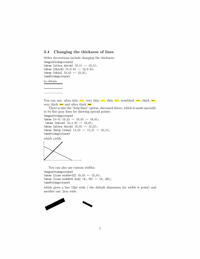
3.4 Changing the thickness of lines

Other decorations include changing the thickness:\begin{tikzpicture}

\draw [ultra thick] (0,1) -- (2,1);

\draw [thick] (0,0.5) -- (2,0.5);

\draw [thin] (0,0) -- (2,0);

\end{tikzpicture}

to obtain

You can use: ultra thin , very thin , thin , semithick , thick ,very thick and ultra thick

There is also the “help lines” option, discussed above, which is made speciallyto be fine gray lines for showing special points:\begin{tikzpicture}

\draw [<->] (0,2) -- (0,0) -- (4,0);

\draw [thick] (0,1.5) -- (3,0);

\draw [ultra thick] (0,0) -- (2,2);

\draw [help lines] (1,0) -- (1,1) -- (0,1);

\end{tikzpicture}

which yields

You can also use custom widths:\begin{tikzpicture}

\draw [line width=12] (0,0) -- (2,0);

\draw [line width=0.2cm] (4,.75) -- (5,.25);

\end{tikzpicture}

which gives a line 12pt wide ( the default dimension for width is point) andanother one .2cm wide:

7

3.5 Dashes and dots

You can also make dotted and dashed lines\begin{tikzpicture}

\draw [dashed, ultra thick] (0,1) -- (2,1);

\draw [dashed] (0, 0.5) -- (2,0.5);

\draw [dotted] (0,0) -- (2,0);

\end{tikzpicture}

This gives:

The top line shows you that you can mix types of decorations. You have lots ofcontrol over the style of your dotted and dashed lines (see the manual).

3.6 Colors

And finally, you can color your lines.\begin{tikzpicture}

\draw [gray] (0,1) -- (2,1);

\draw [red] (0, 0.5) -- (2,0.5);

\draw [blue] (0,0) -- (2,0);

\end{tikzpicture}

This gives

You have direct access to the following colors: red , green , blue , cyan, magenta , yellow , black , gray , darkgray , lightgray ,

brown , lime , olive , orange , pink , purple , teal , violetand white . And you can define all the colors you might want — see the

manual.

3.7 Pictures in the middle of the text

By the way, you may wonder how I included these rectangles in the text. TikZmakes a picture wherever you want; I just typedwherever \begin{tikzpicture} \draw [yellow, line width=6]

(0,0) -- (.5,0); \end{tikzpicture} you want

(To make these constructions easier to type you can use the command \tikz

— see the manual.)

3.8 Curves

You are not limited to straight lines:

8

\begin{tikzpicture}

\draw [blue] (0,0) rectangle (1.5,1);

\draw [red, ultra thick] (3,0.5) circle [radius=0.5];;

\draw [gray] (6,0) arc [radius=1, start angle=45, end angle= 120];

\end{tikzpicture}

This gives:

(The arc is of radius 1, starts at the point (6,0) leaving it at an angle of 45degrees and stops when its slope is 120 degrees — this is not the most convenientnotation!)

You can make paths take smoother turns:\begin{tikzpicture}

\draw [<->, rounded corners, thick, purple] (0,2) -- (0,0) -- (3,0);

\end{tikzpicture}

which gives you

If you want a precise curve you can do it by computing lots of points in aprogram such as Mathematica c© and then putting them into TikZ:\begin{tikzpicture}[xscale=25,yscale=5]

\draw [<->, help lines] (0.6,1.34) -- (0.6,1) -- (1.05,1);

\draw[orange] (0.6, 1.0385) --

(0.61, 1.06372) -- (0.62, 1.08756) -- (0.63, 1.11012) -- (0.64,

1.13147) -- (0.65, 1.15166) -- (0.66, 1.17074) -- (0.67, 1.18874) -- (0.68,

1.20568) -- (0.69, 1.22157) -- (0.7, 1.23643) -- (0.71, 1.25026) -- (0.72,

1.26307) -- (0.73, 1.27486) -- (0.74, 1.28561) -- (0.75, 1.29534) -- (0.76,

1.30402) -- (0.77, 1.31165) -- (0.78, 1.31821) -- (0.79, 1.32369) -- (0.8,

1.32806) -- (0.81, 1.33131) -- (0.82, 1.3334) -- (0.83, 1.33431) -- (0.84,

1.334) -- (0.85, 1.33244) -- (0.86, 1.32956) -- (0.87, 1.32533) -- (0.88,

1.31966) -- (0.89, 1.3125) -- (0.9, 1.30373) -- (0.91, 1.29325) -- (0.92,

1.2809) -- (0.93, 1.26649) -- (0.94, 1.24976) -- (0.95, 1.23032) -- (0.96,

1.2076) -- (0.97, 1.18065) -- (0.98, 1.14763) -- (0.99, 1.1038) -- (0.991,

1.09836) -- (0.992, 1.09261) -- (0.993, 1.0865) -- (0.994, 1.07994) -- (0.995,

1.07282) -- (0.996, 1.06497) -- (0.997, 1.0561) -- (0.998, 1.04563) -- (0.999,

1.03209) -- (0.9991, 1.03042) -- (0.9992, 1.02866) -- (0.9993,

1.02679) -- (0.9994, 1.02478) -- (0.9995, 1.0226) -- (0.9996, 1.02019) -- (0.9997,

1.01747) -- (0.9998, 1.01424) -- (0.9999, 1.01005) -- (0.9999,

1.01005) -- (0.99991, 1.00953) -- (0.99992, 1.00898) -- (0.99993,

1.0084) -- (0.99994, 1.00778) -- (0.99995, 1.0071) -- (0.99996,

1.00634) -- (0.99997, 1.00549) -- (0.99998, 1.00448) -- (0.99999, 1.00317) -- (1,

1) ;

\end{tikzpicture}

9

which gives you

Two remarks:

• This was overkill: I do not need so many points;

• This can also serve as a reminder that one TikZ instruction can be spreadover several lines and cut arbitrarily over several lines. The marker is thesemi-colon, not the end of line!

There are a number of ways by which you can do curves without plotting allthe points. Here is an easy one:\begin{tikzpicture}

\draw[very thick] (0,0) to [out=90,in=195] (2,1.5);

\end{tikzpicture}

This gives us a curve from (0,0) to (2,1.5) which leaves at an angle of 90◦ andarrive at an angle of 195◦:

Note that I had to replace the – by “to”. Notice how the angles work:

• When the curves goes “out” of (0,0), you put a needle with one extremityon the starting point and the other one facing right and you turn it coun-terclockwise until it is tangent to the curve. The angle by which you haveto turn the needle gives you the “out” angle.

• When the curves goes “in” at (2,1.5), you put a needle with one extremityon the arrival point and the other one facing right and you turn it coun-terclockwise until it is tangent to the curve. The angle by which you haveto turn the needle gives you the “in” angle.

As with straight lines you can put several to instructions in the same TikZinstruction:\begin{tikzpicture}

\draw [<->,thick, cyan] (0,0) to [out=90,in=180] (1,1)

to [out=0,in=180] (2.5,0) to [out=0,in=-135] (4,1) ;

\end{tikzpicture}

which gives you

10

Note that we can put arrows on curves also. They are put at the extremities ofthe first and last segments. If you want an arrow on each segment, you have tobuild the curve from individual components.

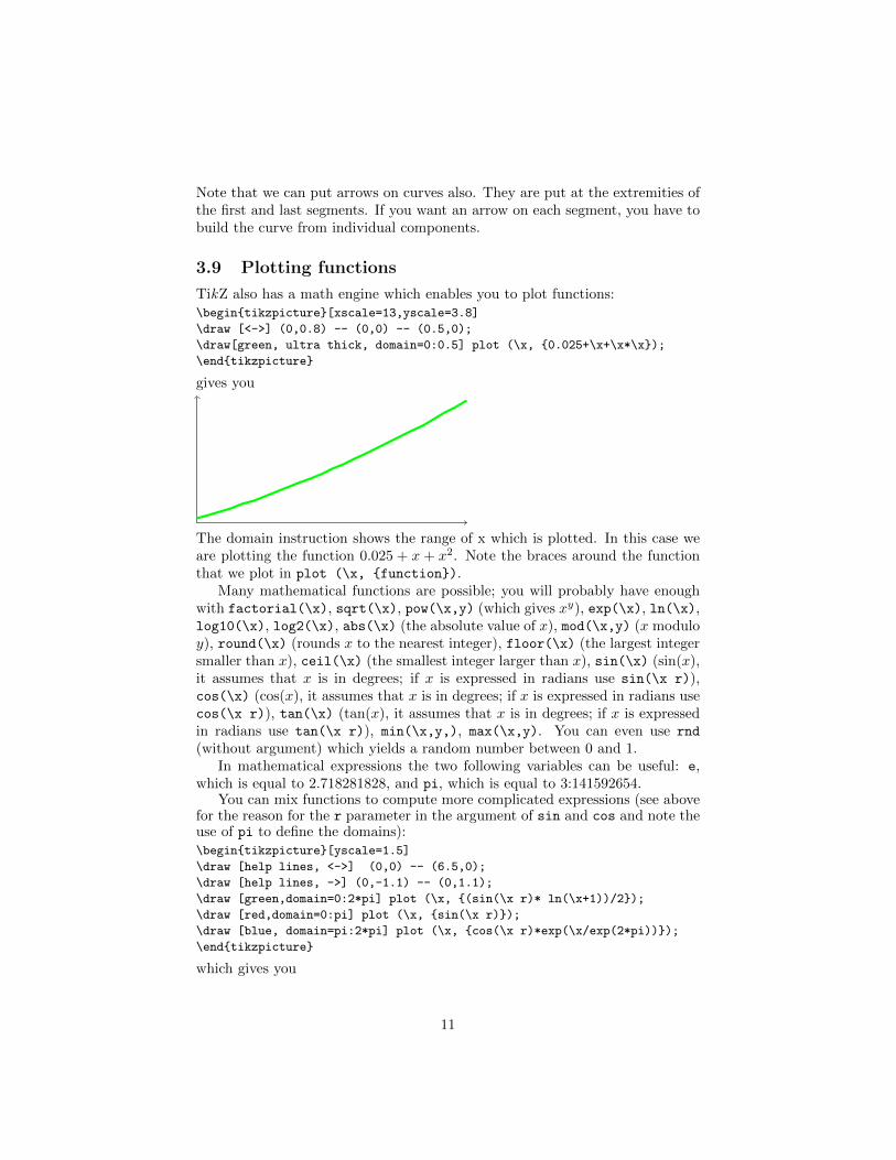
3.9 Plotting functions

TikZ also has a math engine which enables you to plot functions:\begin{tikzpicture}[xscale=13,yscale=3.8]

\draw [<->] (0,0.8) -- (0,0) -- (0.5,0);

\draw[green, ultra thick, domain=0:0.5] plot (\x, {0.025+\x+\x*\x});

\end{tikzpicture}

gives you

The domain instruction shows the range of x which is plotted. In this case weare plotting the function 0.025 + x + x2. Note the braces around the functionthat we plot in plot (\x, {function}).

Many mathematical functions are possible; you will probably have enoughwith factorial(\x), sqrt(\x), pow(\x,y) (which gives xy), exp(\x), ln(\x),log10(\x), log2(\x), abs(\x) (the absolute value of x), mod(\x,y) (x moduloy), round(\x) (rounds x to the nearest integer), floor(\x) (the largest integersmaller than x), ceil(\x) (the smallest integer larger than x), sin(\x) (sin(x),it assumes that x is in degrees; if x is expressed in radians use sin(\x r)),cos(\x) (cos(x), it assumes that x is in degrees; if x is expressed in radians usecos(\x r)), tan(\x) (tan(x), it assumes that x is in degrees; if x is expressedin radians use tan(\x r)), min(\x,y,), max(\x,y). You can even use rnd

(without argument) which yields a random number between 0 and 1.In mathematical expressions the two following variables can be useful: e,

which is equal to 2.718281828, and pi, which is equal to 3:141592654.You can mix functions to compute more complicated expressions (see above

for the reason for the r parameter in the argument of sin and cos and note theuse of pi to define the domains):\begin{tikzpicture}[yscale=1.5]

\draw [help lines, <->] (0,0) -- (6.5,0);

\draw [help lines, ->] (0,-1.1) -- (0,1.1);

\draw [green,domain=0:2*pi] plot (\x, {(sin(\x r)* ln(\x+1))/2});

\draw [red,domain=0:pi] plot (\x, {sin(\x r)});

\draw [blue, domain=pi:2*pi] plot (\x, {cos(\x r)*exp(\x/exp(2*pi))});

\end{tikzpicture}

which gives you

11

4 Filling up areas

4.1 Filling up simple areas

You can also fill paths when they are closed:\begin{tikzpicture}

\draw [fill=red,ultra thick] (0,0) rectangle (1,1);

\draw [fill=red,ultra thick,red] (2,0) rectangle (3,1);

\draw [blue, fill=blue] (4,0) -- (5,1) -- (4.75,0.15) -- (4,0);

\draw [fill] (7,0.5) circle [radius=0.1];

\draw [fill=orange] (9,0) rectangle (11,1);

\draw [fill=white] (9.25,0.25) rectangle (10,1.5);

\end{tikzpicture}

to get

Notice the difference between the first two squares. The second red in [fill=red,ultra thick,red]

tells TikZ to draw the line around the shape in red. We have indicated no colorin the first, so the line is black.

If you do not want to see the outline at all, replace the \draw command by\path:\begin{tikzpicture}

\path [fill=gray] (0,0) rectangle (1.5,1);

\draw [fill=yellow] (2,0) rectangle (3.5,1);

\end{tikzpicture}

gives you

Of course, we could have replaced the first line by \draw [fill=yellow,yellow] (0,0) rectangle (1.5,1);:we would have obtained a square like the second one, except for the fact that itis surrounded by a yellow line.

12

4.2 Filling up arbitrary areas

The content in this subsection are not necessary to understand the rest of thedocument. You can skip it at first reading. (But example 8.5 uses these tech-niques.)

You can draw paths which mix the -- and the to constructions above. Thisis useful for filling up strange looking areas.\begin{tikzpicture}

\draw [ultra thick] (0,0) to [out=87,in=150] (1,1) -- (.85,.15) -- (0,0);

\draw [ultra thick, fill=purple] (2,0) to [out=87,in=150] (3,1) -- (2.85,.15) -- (2,0);

\path [fill=purple] (4,0) to [out=87,in=150] (5,1) -- (4.85,.15) -- (4,0);

\end{tikzpicture}

to get

Actually if you put the to constructions without any “options” you get astraight line:\begin{tikzpicture}

\draw [ultra thick] (0,0) to (1,1) to (.85,.15) to (0,0);

\end{tikzpicture}

gives you

5 Putting labels in pictures

When you do a picture, in 99% of cases you also need to put labels. This iseasy. Let us start by seeing how we would place some text in a picture.\begin{tikzpicture}

\draw [thick, <->] (0,2) -- (0,0) -- (2,0);

\node at (1,1) {yes};

\end{tikzpicture}

yields

yes

Notice how the “yes” is positioned: the center of its “baseline” is at (1,1).Sometimes you want a label to be situated relative to a point. TikZ has neat

commands for this. For instance you can write

13

\begin{tikzpicture}

\draw [thick, <->] (0,2) -- (0,0) -- (2,0);

\draw[fill] (1,1) circle [radius=0.025];

\node [below] at (1,1) {below};

\end{tikzpicture}

to get

below

You are not limited to put things below a point:\begin{tikzpicture}

\draw [thick, <->] (0,2) -- (0,0) -- (2,0);

\draw[fill] (1,1) circle [radius=0.025];

\node [below] at (1,1) {below};

\node [above] at (1,1) {above};

\node [left] at (1,1) {left};

\node [right] at (1,1) {right};

\end{tikzpicture}

yields

below

aboveleft right

And, you can also mix and match\begin{tikzpicture}[scale=2]

\draw [thick, <->] (0,1) -- (0,0) -- (1,0);

\draw[fill] (1,1) circle [radius=0.025];

\node [below right, red] at (.5,.75) {below right};

\node [above left, green] at (.5,.75) {above left};

\node [below left, purple] at (.5,.75) {below left};

\node [above right, magenta] at (.5,.75) {above right};

\end{tikzpicture}

yields

below right

above left

below left

above right

This makes it possible to label axes and points:\begin{tikzpicture}[xscale=3, yscale=1.5]

\draw [thick, <->] (0,1) -- (0,0) -- (1,0);

\node [below right] at (1,0) {$x$};

14

\node [left] at (0,1) {$y$};

\draw[fill] (.4,.6) circle [radius=.5pt];

\node[above right] (.4,.6) {$A$};

\end{tikzpicture}

gives you

x

yA

You can avoid some typing by mixing nodes in the middle of paths. Forinstance the last figure could have been written as follows:\begin{tikzpicture}[xscale=3, yscale]

\draw [thick, <->] (0,1) node [left] {$y$}

-- (0,0) -- (1,0) node [below right] {$x$};

\draw[fill] (.4,.6) circle [radius=.5pt]

node[above right] (.4,.6) {$A$};

\end{tikzpicture}

which would have given exactly the same result. Note that the node is put afterthe point to which it is attached and that we suppress the \ in \node.

Sometimes, you may want to put several lines in your “node” (this is con-venient when drawing time lines for instance). This can be done by using thestandard LATEX \\ for indicating a new line but you must tell TikZ how to alignthings. Type\begin{tikzpicture}[xscale=1.3]

\draw [thick] (0,0) -- (9,0);

\draw (0,-.2) -- (0, .2);

\draw (3,-.2) -- (3, .2);

\draw (6,-.2) -- (6, .2);

\draw (9,-.2) -- (9, .2);

\node[align=left, below] at (1.5,-.5)%

{This happens\\in period 1\\and is aligned\\ left};

\node[align=center, below] at (4.5,-.5)%

{This happens\\in period 2\\and is centered};

\node[align=right, below] at (7.5,-.5)%

{This happens\\in period 2\\and is right\\aligned};

\end{tikzpicture}

to obtain

This happensin period 1and is alignedleft

This happensin period 2

and is centered

This happensin period 2and is right

aligned

Without the option align= TikZ will make one big line. If I made the mistaketo write

15

\begin{tikzpicture}

\draw [->] (0,0) -- (2,0);

\node [right] at (2,0) {above\\below};

\end{tikzpicture}

I would have obtained

abovebelow

The TikZ manual will give you information about the way in which you cancontrol more precisely the position and shapes of the labels, and also on the

way in which you can put labels on lines and curves as inlabel .

6 Integration with Beamer

TikZ works very well with Beamer (they were written by the same person!). Inparticular it is very easy to uncover figures progressively. For instance\begin{frame}

a few lines

\begin{center}

\begin{tikzpicture}

\draw [blue, ultra thick] (-1,2) -- (6,3);

\uncover<1>{\draw [green,thick] (-4,3) -- (2,2.5);}

\uncover<2>{\draw [red,thick] (0,0) -- (0,5);}

\end{tikzpicture}

\end{center}

and something under.

\end{frame}

gives you two slides:

a few lines

and something under.

a few lines

and something under.

It is important to use \uncover and \cover (or, nearly equivalently, \visibleand \invisible) rather than \only. If I replace \uncover by \only in thecode above I get

16

a few lines

and something under.

a few lines

and something under.

Notice how the text changes position. With \uncover the lines are “drawn” onall the slides but made invisible when not called for. With \only the lines areonly drawn when called for.

7 Hints and tricks

• It takes some time to draw figures. And it is normal to make mistakes.Proceed by trial and error, compiling your code often.

• If you have problems placing things, it is useful to draw a grid; you cancomment it out when compiling the final version. Put the grid as the firstinstruction in the picture, so that it does not overwrite the interestingpart! (There are lots of possible options for the grid: see the manual.)

8 Examples

A few examples.

8.1 Hotelling

8.1.1 The whole picture

0 a = b = 1/2 1

\begin{tikzpicture}[xscale=8]

\draw[-][draw=red, very thick] (0,0) -- (.5,0);

\draw[-][draw=green, very thick] (.5,0) -- (1,0);

\draw [thick] (0,-.1) node[below]{0} -- (0,0.1);

\draw [thick] (0.5,-.1) node[below]{$a=b=1/2$} -- (0.5,0.1);

\draw [thick] (1,-.1) node[below]{1} -- (1,0.1);

\end{tikzpicture}

17

8.1.2 Step by step

\draw[-][draw=red, very thick] (0,0) -- (.5,0);

\draw[-][draw=green, very thick] (.5,0) -- (1,0);

\draw [thick] (0,-.1) node[below]{0} -- (0,0.1);0

\draw [thick] (0.5,-.1) node[below]{$a=b=1/2$} -- (0.5,0.1);0 a = b = 1/2

\draw [thick] (1,-.1) node[below]{1} -- (1,0.1);0 a = b = 1/2 1

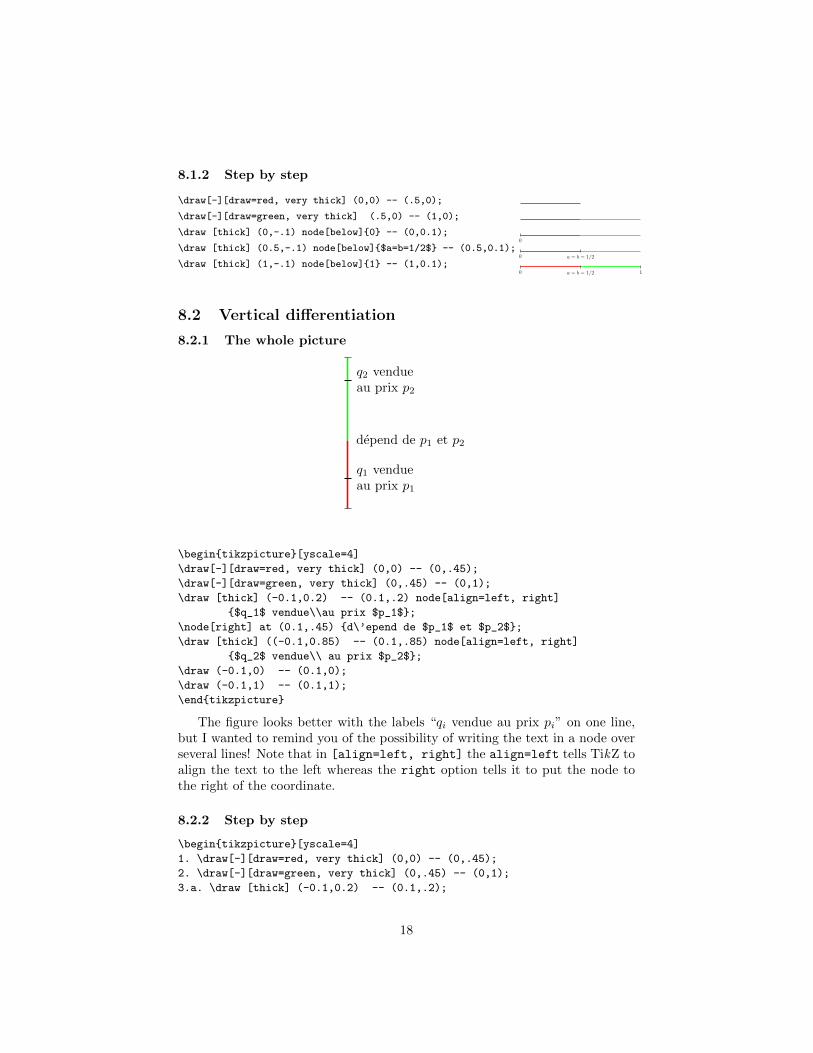
8.2 Vertical differentiation

8.2.1 The whole picture

q1 vendueau prix p1

depend de p1 et p2

q2 vendueau prix p2

\begin{tikzpicture}[yscale=4]

\draw[-][draw=red, very thick] (0,0) -- (0,.45);

\draw[-][draw=green, very thick] (0,.45) -- (0,1);

\draw [thick] (-0.1,0.2) -- (0.1,.2) node[align=left, right]

{$q_1$ vendue\\au prix $p_1$};

\node[right] at (0.1,.45) {d\’epend de $p_1$ et $p_2$};

\draw [thick] ((-0.1,0.85) -- (0.1,.85) node[align=left, right]

{$q_2$ vendue\\ au prix $p_2$};

\draw (-0.1,0) -- (0.1,0);

\draw (-0.1,1) -- (0.1,1);

\end{tikzpicture}

The figure looks better with the labels “qi vendue au prix pi” on one line,but I wanted to remind you of the possibility of writing the text in a node overseveral lines! Note that in [align=left, right] the align=left tells TikZ toalign the text to the left whereas the right option tells it to put the node tothe right of the coordinate.

8.2.2 Step by step

\begin{tikzpicture}[yscale=4]

1. \draw[-][draw=red, very thick] (0,0) -- (0,.45);

2. \draw[-][draw=green, very thick] (0,.45) -- (0,1);

3.a. \draw [thick] (-0.1,0.2) -- (0.1,.2);

18

3. \draw [thick] (-0.1,0.2) -- (0.1,.2) node[align=left, right]

{$q_1$ vendue\\au prix $p_1$};

4. \node[right] at (0.1,.45) {d\’epend de $p_1$ et $p_2$};

4. \draw [thick] ((-0.1,0.85) -- (0.1,.85) node[align=left, right]

{$q_2$ vendue\\ au prix $p_2$};

5. \draw (-0.1,0) -- (0.1,0);

5. \draw (-0.1,1) -- (0.1,1);

\end{tikzpicture}

1 2 3.a

q1 vendueau prix p1

3

q1 vendueau prix p1

depend de p1 et p2

q2 vendueau prix p2

4

q1 vendueau prix p1

depend de p1 et p2

q2 vendueau prix p2

5

8.3 A curve

8.3.1 The whole picture

q

V (q)

\begin{center}

\begin{tikzpicture}

\draw[<->] (6,0) node[below]{$q$} -- (0,0) --

(0,6) node[left]{$V(q)$};

\draw[very thick] (0,0) to [out=90,in=145] (5,4.5);

\end{tikzpicture}

\end{center}

19

8.3.2 Step by step

\begin{tikzpicture}

1.a. \draw[<->] (6,0) -- (0,0) --

(0,6);

1. \draw[<->] (6,0) node[below]{$q$} -- (0,0) --

(0,6) node[left]{$V(q)$};

2. \draw[very thick] (0,0) to [out=90,in=145] (5,4.5);

\end{tikzpicture}

1.a

q

V (q)

1

q

V (q)

3

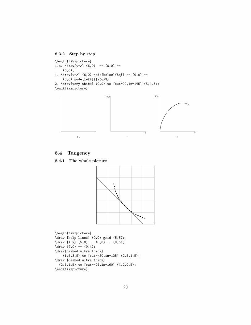
8.4 Tangency

8.4.1 The whole picture

\begin{tikzpicture}

\draw [help lines] (0,0) grid (5,5);

\draw [<->] (5,0) -- (0,0) -- (0,5);

\draw (4,0) -- (0,4);

\draw[dashed,ultra thick]

(1.5,3.5) to [out=-80,in=135] (2.5,1.5);

\draw [dashed,ultra thick]

(2.5,1.5) to [out=-45,in=160] (4.2,0.5);

\end{tikzpicture}

20

You have recognized a consumer! Note the use of “in” and “to” to get thetangents. We could have made this a bit more compact by writing the dashedline in one instruction:\draw[dashed,ultra thick]

(1.5,3.5) to[out=-80,in=135] (2.5,1.5)

to [out=-45,in=160] (4.2,0.5);

Notice also that the curves goes “in” (2.5,1.5) at an angle of 135◦ and goes “out”at an angle of 45◦. This is consistent with the behavior explained on page 10.

8.4.2 Step by step

\begin{tikzpicture}

1. \draw [help lines] (0,0) grid (5,5);

1. \draw [<->] (5,0) -- (0,0) -- (0,5);

1. \draw (4,0) -- (0,4);

2. \draw[dashed,ultra thick]

(1.5,3.5) to [out=-80,in=135] (2.5,1.5);

3. \draw [dashed,ultra thick]

(2.5,1.5) to [out=-45,in=160] (4.2,0.5);

\end{tikzpicture}

1 2 3

21

8.5 Consumer surplus

8.5.1 The whole picture

P

(0,0) Q

P ∗ = .8

Q∗ = 3

\begin{tikzpicture}

\path [fill=yellow] (0,0) -- (0,5) to [out=-80, in=160]

(3,.8) -- (3,0) -- (0,0);

\draw [<->] (0,6) node [left] {$P$} -- (0,0)

node [below left] {(0,0)} -- (7,0) node [below] {$Q$};

\draw [ultra thick, dashed] (0,.8) node [left] {$P^*=.8$} -- (3,.8)

-- (3,0) node [below] {$Q^*=3$};

\draw [fill] (3,.8) circle [radius=.1];

\draw [thick] (0,5) to [out=-80, in=160] (3,.8) to

[out=-20, in=175] (6,0);

\end{tikzpicture}

Note that I color the filled area before drawing the lines, to make sure thatthose come on top and are visible. (There is, of course, no serious reason forthe P ∗ and the Q∗ to be equal to the “real” coordinates of the circled point inthe picture, except to help you understand what is happening.)

8.5.2 Step by step

\begin{tikzpicture}

1. \path [fill=yellow] (0,0) -- (0,5) to [out=-80, in=160]

(3,.8) -- (3,0) -- (0,0);

2. \draw [<->] (0,6) node [left] {$P$} -- (0,0)

node [below left] {(0,0)} -- (7,0) node [below] {$Q$};

2. \draw [ultra thick, dashed] (0,.8) node [left] {$P^*=.8$} -- (3,.8)

-- (3,0) node [below] {$Q^*=3$};

2. \draw [fill] (3,.8) circle [radius=.1];

3. \draw [thick] (0,5) to [out=-80, in=160] (3,.8) to

22

[out=-20, in=175] (6,0);

\end{tikzpicture}

1

P

(0,0) Q

P ∗ = .8

Q∗ = 3

2

P

(0,0) Q

P ∗ = .8

Q∗ = 3

3

8.6 Plotting lots of curves

EUR

q

v1(x)

v2(x)

2 min[v1, v2]

\begin{center}

\begin{tikzpicture}[domain=0:0.5,xscale=13,yscale=3.8]

\draw[<->] (0,2) node[left]{EUR}-- (0,0) -- (.7,0) node[below] {$q$};

\draw[red] plot (\x, {0.25+\x/2+\x*\x/2}) node[right] {$v_1(x)$};

\draw[green] plot (\x, {0.025+\x+\x*\x}) node[right] {$v_2(x)$};

\draw[thin, dashed] plot (\x, {0.275+1.5*\x+1.5*\x*\x}) ;

\draw[thick,domain=0:0.33666] plot (\x, {0.05+2*\x+2*\x*\x}) ;

\draw[thick,domain=0.33666:0.5]

plot (\x, {0.5+\x+\x*\x}) node[right] {$2\min[v_1,v_2]$};

\end{tikzpicture}

\end{center}

You should be able to figure it out. Note that I can also attach nodes to theplots of mathematical functions.

23

9 Conclusion

TikZ is a very large program which can do lots of things. You will find commandsto draw hierarchial trees, to draw lots of different types of shapes, to do someelementary programming, to align elements of a picture in a matrix frame, todecorate nodes, to compute the intersections of paths, etc. The main messageis “if it is not in these notes, it is most probably somewhere in the manual”.

24