A Very Fast Learning Method for Neural Networks Based on ...

Journal of Machine Learning Research 7 (2006) 1159–1182 Submitted 2/05; Revised 4/06; Published 7/06

A Very Fast Learning Method for Neural NetworksBased on Sensitivity Analysis

Enrique Castillo CASTIE@UNICAN .ES

Department of Applied Mathematics and Computational SciencesUniversity of Cantabria and University of Castilla-La ManchaAvda de Los Castros s/n, 39005 Santander, Spain

Bertha Guijarro-Berdi nas [email protected]

Oscar Fontenla-Romero [email protected]

Amparo Alonso-Betanzos [email protected]

Department of Computer ScienceFaculty of Informatics, University of A CorunaCampus de Elvina s/n, 15071 A Coruna, Spain

Editor: Yoshua Bengio

AbstractThis paper introduces a learning method for two-layer feedforward neural networks based on sen-sitivity analysis, which uses a linear training algorithm for each of the two layers. First, randomvalues are assigned to the outputs of the first layer; later, these initial values are updated based onsensitivity formulas, which use the weights in each of the layers; the process is repeated until con-vergence. Since these weights are learnt solving a linear system of equations, there is an importantsaving in computational time. The method also gives the local sensitivities of the least square errorswith respect to input and output data, with no extra computational cost, because the necessary in-formation becomes available without extra calculations. This method, called the Sensitivity-BasedLinear Learning Method, can also be used to provide an initial set of weights, which significantlyimproves the behavior of other learning algorithms. The theoretical basis for the method is givenand its performance is illustrated by its application to several examples in which it is compared withseveral learning algorithms and well known data sets. The results have shown a learning speed gen-erally faster than other existing methods. In addition, it can be used as an initialization tool for otherwell known methods with significant improvements.

Keywords: supervised learning, neural networks, linear optimization, least-squares, initializationmethod, sensitivity analysis

1. Introduction

There are many alternative learning methods and variants for neural networks. In the case of feedfor-ward multilayer networks the first successful algorithm was the classical backpropagation (Rumel-hart et al., 1986). Although this approach is very useful for the learning process of this kind ofneural networks it has two main drawbacks:

• Convergence to local minima.

• Slow learning speed.

c©2006 Enrique Castillo, Bertha Guijarro-Berdinas, Oscar Fontenla-Romero and Amparo Alonso-Betanzos.

CASTILLO , GUIJARRO-BERDINAS, FONTENLA-ROMERO AND ALONSO-BETANZOS

In order to solve these problems, several variations of the initial algorithm and also new methodshave been proposed. Focusing the attention on the problem of the slow learning speed, some algo-rithms have been developed to accelerate it:

• Modifications of the standard algorithms: Some relevant modifications of the backpropaga-tion method have been proposed. Sperduti and Antonina (1993) extend the backpropagationframework by adding a gradient descent to the sigmoids steepness parameters. Ihm and Park(1999) present a novel fast learning algorithm to avoid the slow convergence due to weightoscillations at the error surface narrow valleys. To overcome this difficulty they derive anew gradient term by modifying the original one with an estimated downward direction atvalleys. Also, stochastic backpropagation—which is opposite to batch learning and updatesthe weights in each iteration—often decreases the convergence time, and is specially rec-ommended when dealing with large data sets on classification problems (see LeCun et al.,1998).

• Methods based on linear least-squares: Some algorithms based on linear least-squares meth-ods have been proposed to initialize or train feedforward neural networks (Biegler-Konig andBarmann, 1993; Pethel et al., 1993; Yam et al., 1997; Cherkassky and Mulier, 1998; Castilloet al., 2002; Fontenla-Romero et al., 2003). These methods are mostly based on minimiz-ing the mean squared error (MSE) between the signal of an output neuron, before the outputnonlinearity, and a modified desired output, which is exactly the actual desired output passedthrough the inverse of the nonlinearity. Specifically, in (Castillo et al., 2002)a method forlearning a single layer neural network by solving a linear system of equations is proposed.This method is also used in (Fontenla-Romero et al., 2003) to learn the last layer of a neuralnetwork, while the rest of the layers are updated employing any other non-linear algorithm(for example, conjugate gradient). Again, the linear method in (Castillo et al., 2002) is thebasis for the learning algorithm proposed in this article, although in this case all layers arelearnt by using a system of linear equations.

• Second order methods: The use of second derivatives has been proposed to increase the con-vergence speed in several works (Battiti, 1992; Buntine and Weigend, 1993; Parker, 1987). Ithas been demonstrated (LeCun et al., 1991) that these methods are more efficient, in terms oflearning speed, than the methods based only on the gradient descent technique. In fact, secondorder methods are among the fastest learning algorithms. Some of the most relevant exam-ples of this type of methods are the quasi-Newton, Levenberg-Marquardt (Hagan and Men-haj, 1994; Levenberg, 1944; Marquardt, 1963) and the conjugate gradient algorithms (Beale,1972). Quasi-Newton methods use a local quadratic approximation of the error function, likethe Newton’s method, but they employ an approximation of the inverse of the hessian matrixto update the weights, thus getting a lowest computational cost. The two most common up-dating procedures are the Davidson-Fletcher-Powell (DFP) and Broyden-Fletcher-Goldfarb-Shanno (BFGS) (Dennis and Schnabel, 1983). The Levenberg-Marquardt method combines,in the same weight updating rule, both the gradient and the Gauss-Newton approximation ofthe hessian of the error function. The influence of each term is determinedby an adaptiveparameter, which is automatically updated. Regarding the conjugate gradientmethods, theyuse, at each iteration of the algorithm, different search directions in a waythat the compo-nent of the gradient is parallel to the previous search direction. Several algorithms based on

1160

A V ERY FAST LEARNING METHOD FORNEURAL NETWORKSBASED ON SENSITIVITY ANALYSIS

conjugate directions were proposed such as the Fletcher-Reeves (Fletcher and Reeves, 1964;Hagan et al., 1996), Polak-Ribiere (Fletcher and Reeves, 1964; Hagan et al., 1996), Powell-Beale (Powell, 1977) and scaled conjugate gradient algorithms (Moller, 1993). Also, basedon these previous approaches, several new algorithms have been developed, like those ofChella et al. (1993) and Wilamowski et al. (2001). Nevertheless, second-order methods arenot practicable for large neural networks trained in batch mode, althoughsome attempts toreduce their computational cost or to obtain stochastic versions have appeared (LeCun et al.,1998; Schraudolph, 2002).

• Adaptive step size: In the standard backpropagation method the learning rate, which deter-mines the magnitude of the changes in the weights for each iteration of the algorithm, is fixedat the beginning of the learning process. Several heuristic methods for the dynamical adapta-tion of the learning rate have been developed (Hush and Salas, 1988; Jacobs, 1988; Vogl et al.,1988). Other interesting algorithm is the superSAB, proposed by Tollenaere (Tollenaere,1990). This method is an adaptive acceleration strategy for error backpropagation learningthat converges faster than the gradient descent with optimal step size value, reducing the sen-sitivity to parameter values. Moreover, in (Weir, 1991) a method for the self-determination ofthis parameter has also been presented. More recently, in Orr and Leen (1996), an algorithmfor fast stochastic gradient descent, which uses a nonlinear adaptivemomentum scheme to op-timize the slow convergence rate was proposed. Also, in Almeida et al. (1999), a new methodfor step size adaptation in stochastic gradient optimization was presented. This method usesindependent step sizes for all parameters and adapts them employing the available derivativesestimates in the gradient optimization procedure. Additionally, a new online algorithm forlocal learning rate adaptation was proposed (Schraudolph, 2002).

• Appropriate weights initialization: The starting point of the algorithm, determined by theinitial set of weights, also influences the method convergence speed. Thus, several solutionsfor the appropriate initialization of weights have been proposed. Nguyen and Widrow assigneach hidden processing element an approximate portion of the range of thedesired response(Nguyen and Widrow, 1990), and Drago and Ridella use the statistically controlled activationweight initialization, which aims to prevent neurons from saturation during theadaptationprocess by estimating the maximum value that the weights should take initially (DragoandRidella, 1992). Also, in (Ridella et al., 1997), an analytical technique, to initialize the weightsof a multilayer perceptron with vector quantization (VQ) prototypes given the equivalencebetween circular backpropagation networks and VQ classifiers, has been proposed.

• Rescaling of variables: The error signal involves the derivative of the neural function, whichis multiplied in each layer. Therefore, the elements of the Jacobian matrix can differ greatlyin magnitude for different layers. To solve this problem Rigler et al. (1991) have proposed arescaling of these elements.

On the other hand, sensitivity analysis is a very useful technique for deriving how and howmuch the solution to a given problem depends on data (see, for example, Castillo et al., 1997,1999, 2000). However, in this paper we show that sensitivity formulas can also be used for learning,and a novel supervised learning algorithm for two-layer feedforwardneural networks that presents ahigh convergence speed is proposed. This algorithm, the Sensitivity-Based Linear Learning Method

1161


(SBLLM), is based on the use of the sensitivities of each layer’s parameters with respect to its inputsand outputs, and also on the use of independent systems of linear equations for each layer, to obtainthe optimal values of its parameters. In addition, this algorithm gives the sensitivities of the sum ofsquared errors with respect to the input and output data.

The paper is structured as follows. In Section 2 a method for learning one layer neural networksthat consists of solving a system of linear equations is presented, and formulas for the sensitivitiesof the sum of squared errors with respect to the input and output data are derived. In Section 3 theSBLLM method, which uses the previous linear method to learn the parameters of two-layer neuralnetworks and the sensitivities of the total sum of squared errors with respect to the intermediateoutput layer values, which are modified using a standard gradient formulauntil convergence, ispresented. In Section 4 the proposed method is illustrated by its application to several practicalproblems, and also it is compared with some other fast learning methods. In Section 5 the SBLLMmethod is presented as an initialization tool to be used with other learning methods.In Section 6these results are discussed and some future work lines are presented. Finally, in Section 7 someconclusions and recommendations are given.

2. One-Layer Neural Networks

Consider the one-layer network in Figure 1. The set of equations relatinginputs and outputs is givenby

y js = f j

(

I

∑i=0

w ji xis

)

; j = 1,2, . . . ,J; s= 1,2, . . . ,S,

whereI is the number of inputs,J the number of outputs,x0s = 1, w ji are the weights associatedwith neuronj andS is the number of data points.

f 1

f 2

f J

...

y 1S

y 2S

y JS

x 1S

x 2S

x IS

...

w 11

w 21 w J1

w 12

w 22

w J2

w 1I w 2I

w JI

w J0 w 10

w 20

x 0S =1

+

+

+

Figure 1: One-layer feedforward neural network.

To learn the weightsw ji , the following sum of squared errors between the real and the desiredoutput of the networks is usually minimized:

1162


P =S

∑s=1

J

∑j=1

δ2js =

S

∑s=1

J

∑j=1

(

y js− f j

(

I

∑i=0

w ji xis

))2

.

Assuming that the nonlinear activation functions,f j , are invertible (as it is the case for the mostcommonly employed functions), alternatively, one can minimize the sum of squared errors beforethe nonlinear activation functions (Castillo et al., 2002), that is,

Q =S∑

s=1

J∑j=1

ε2js =

S∑

s=1

J∑j=1

(

I∑

i=0w ji xis− f−1

j (y js)

)2

, (1)

which leads to the system of equations:

∂Q∂w jp

= 2S

∑s=1

(

I

∑i=0

w ji xis− f−1j (y js)

)

xps = 0; p = 0,1, . . . , I ; ∀ j,

that is,

I

∑i=0

w ji

S

∑s=1

xisxps =S

∑s=1

f−1j (y js)xps; p = 0,1, . . . , I ; ∀ j

or

I

∑i=0

Apiw ji = bp j; p = 0,1, . . . , I ; ∀ j, (2)

where

Api =S

∑s=1

xisxps; p = 0,1, . . . , I ; ∀i

bp j =S

∑s=1

f−1j (y js)xps; p = 0,1, . . . , I ; ∀ j.

Moreover, for the neural network shown in Figure 1, the sensitivities (see Castillo et al., 2001,2004, 2006) of the new cost function,Q, with respect to the output and input data can be obtainedas:

∂Q∂ypq

= −

2

(

I∑

i=0wpixiq − f−1

p (ypq)

)

f ′p(ypq); ∀p,q (3)

∂Q∂xpq

= 2J

∑j=1

(

I

∑i=0

w ji xiq − f−1j (y jq)

)

w jp; ∀p,q. (4)

1163


3. The Proposed Sensitivity-Based Linear Learning Method

The learning method and the sensitivity formulas given in the previous sectioncan be used to de-velop a new learning method for two-layer feedforward neural networks, as it is described below.

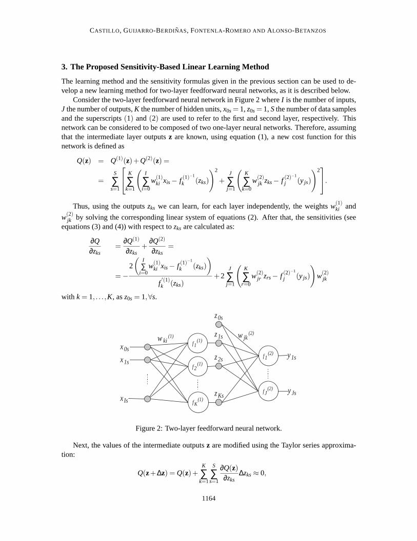
Consider the two-layer feedforward neural network in Figure 2 whereI is the number of inputs,J the number of outputs,K the number of hidden units,x0s = 1,z0s = 1,Sthe number of data samplesand the superscripts(1) and(2) are used to refer to the first and second layer, respectively. Thisnetwork can be considered to be composed of two one-layer neural networks. Therefore, assumingthat the intermediate layer outputsz are known, using equation (1), a new cost function for thisnetwork is defined as

Q(z) = Q(1)(z)+Q(2)(z) =

=S

∑s=1

K

∑k=1

(

I

∑i=0

w(1)ki xis− f (1)−1

k (zks)

)2

+J

∑j=1

(

K

∑k=0

w(2)jk zks− f (2)−1

j (y js)

)2

.

Thus, using the outputszks we can learn, for each layer independently, the weightsw(1)ki and

w(2)jk by solving the corresponding linear system of equations (2). After that, the sensitivities (see

equations (3) and (4)) with respect tozks are calculated as:

∂Q∂zks

=∂Q(1)

∂zks+

∂Q(2)

∂zks=

= −

2

(

I∑

i=0w(1)

ki xis− f (1)−1

k (zks)

)

f′(1)k (zks)

+2J

∑j=1

(

K

∑r=0

w(2)jr zrs− f (2)−1

j (y js)

)

w(2)jk

with k = 1, . . . ,K, asz0s = 1,∀s.

f K (1)

f 2 (1)

f 1 (1) w ki

(1)

f 1 (2)

f J (2)

x 1s

x 0s

x Is

y 1s

y Js

w jk (2) z 1s

z 2s

z Ks

z 0s

Figure 2: Two-layer feedforward neural network.

Next, the values of the intermediate outputsz are modified using the Taylor series approxima-tion:

Q(z+∆z) = Q(z)+K

∑k=1

S

∑s=1

∂Q(z)∂zks

∆zks≈ 0,

1164


which leads to the following increments

∆z = −ρQ(z)

||∇Q||2∇Q, (5)

whereρ is a relaxation factor or step size.

The proposed method is summarized in the following algorithm.

Algorithm SBLLM

Input. The data set (input,xis, and desired data,y js), two threshold errors (ε andε′) to controlconvergence, and a step sizeρ .

Output. The weights of the two layers and the sensitivities of the sum of squared errors withrespect to input and output data.

Step 0: Initialization. Assign to the outputs of the intermediate layer the output associated withsome random weightsw(1)(0) plus a small random error, that is:

zks = f (1)k

(

I

∑i=0

w(1)ki (0)xis

)

+ εks; εks∼U(−η,η);k = 1, . . . ,K,

whereη is a small number, and initializeQprevious andMSEprevious to some large number, whereMSEmeasures the error between the obtained and the desired output.

Step 1: Subproblem solution.Learn the weights of layers 1 and 2 and the associated sensitivitiessolving the corresponding systems of equations, that is,

I

∑i=0

A(1)pi w(1)

ki = b(1)pk

K

∑k=0

A(2)qk w(2)

jk = b(2)q j ,

whereA(1)pi =

S∑

s=1xisxps; b(1)

pk =S∑

s=1f (1)−1

k (zks)xps; p = 0,1, . . . , I ; k = 1,2, . . . ,K

andA(2)qk =

S∑

s=1zkszqs; b(2)

q j =S∑

s=1f (2)−1

j (y js)zqs; q = 0,1, . . . ,K; ∀ j.

Step 2: Evaluate the sum of squared errors.EvaluateQ using

Q(z) = Q(1)(z)+Q(2)(z)

=S

∑s=1

K

∑k=1

(

I

∑i=0

w(1)ki xis− f (1)−1

k (zks)

)2

+J

∑j=1

(

K

∑k=0

w(2)jk zks− f (2)−1

j (y js)

)2

and evaluate also theMSE.

1165


Step 3: Convergence checking.If |Q−Qprevious| < ε or |MSEprevious−MSE| < ε′ stop and returnthe weights and the sensitivities. Otherwise, continue with Step 4.

Step 4: Check improvement ofQ. If Q > Qprevious reduce the value ofρ, that is,ρ = ρ/2, andreturn to the previous position, that is, restore the weights,z= zprevious, Q= Qpreviousand go to Step5. Otherwise, store the values ofQ andz, that is,Qprevious= Q, MSEprevious= MSEandzprevious= zand obtain the sensitivities using:

∂Q∂zks

= −

2

(

I∑

i=0w(1)

ki xis− f (1)−1

k (zks)

)

f′(1)k (zks)

+2J

∑j=1

(

K

∑r=0

w(2)jr zrs− f (2)−1

j (y js)

)

w(2)jk ;k = 1, . . . ,K.

Step 5: Update intermediate outputs. Using the Taylor series approximation in equation (5),update the intermediate outputs as

z = z−ρQ(z)

||∇Q||2∇Q

and go to Step 1.The complexity of this method is determined by the complexity of Step 1 which solves alinear

system of equations for each network’s layer. Several efficient methods can be used to solve thiskind of systems with a complexity ofO(n2), wheren is the number of unknowns. Therefore, theresulting complexity of the proposed learning method is alsoO(n2), beingn the number of weightsof the network.

4. Examples of Applications of the SBLLM to Train Neural Networks

In this section the proposed method, SBLLM,1 is illustrated by its application to five system iden-tification problems. Two of them are small/medium size problems (Dow-Jones andLeuven compe-tition time series), while the other three used large data sets and networks (Lorenz time series, andthe MNIST and UCI Forest databases). Also, in order to check the performance of the SBLLM,it was compared with five of the most popular learning methods. Three of these methods are thegradient descent (GD), the gradient descent with adaptive momentum and step sizes (GDX), andthe stochastic gradient descent (SGD), whose complexity isO(n). The other methods are the scaledconjugated gradient (SCG), with complexity ofO(n2), and the Levenberg-Marquardt (LM) (com-plexity of O(n3)). All experiments were carried out in MATLABR© running on a Compaq HPC 320with an Alpha EV68 1 GHz processor and 4GB of memory. For each experiment all the learningmethods shared the following conditions:

• The network topology and neural functions. In all cases, the logistic function was used forhidden neurons, while for output neurons the linear function was used for regression problemsand the logistic function was used for classification problems. It is important toremark thatthe aim here is not to investigate the optimal topology, but to check the performance of thealgorithms in both small and large networks.

1. MATLAB R© demo code available at http://www.dc.fi.udc.es/lidia/downloads/SBLLM.

1166


• Initial step size equal to 0.05, except for the stochastic gradient descent. In this last case, weused a step size in the interval[0.005,0.2]. These step sizes were tuned in order to obtaingood results.

• The input data set was normalized (mean = 0 and standard deviation = 1).

• Several simulations were performed using for each one a different setof initial weights. Thisinitial set was the same for all the algorithms (except for the SBLLM), and was obtained bythe Nguyen-Widrow (Nguyen and Widrow, 1990) initialization method.

• Finally, statistical tests were performed in order to check whether the differences in accuracyand speed were significant among the different training algorithms. Specifically, first thenon-parametric Kruskal-Wallis test (Hollander and Wolfe, 1973) was applied to check thehypothesis that all mean performances are equal. When this hypothesis is rejected, a multiplecomparison test of means based on the Tukey’s honestly significant difference criterion (Hsu,1996) was applied to know which pairs of means are different. In all cases, a significancelevel of 0.05 was used.

4.1 Dow-Jones Time Series

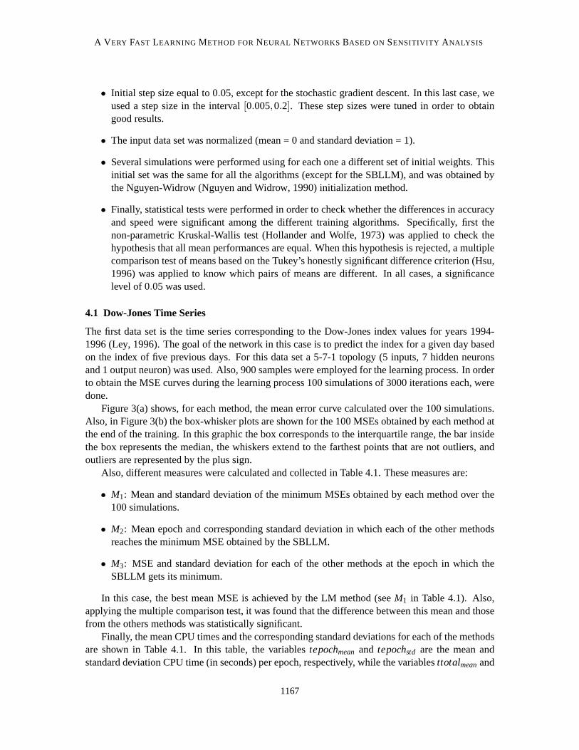
The first data set is the time series corresponding to the Dow-Jones index values for years 1994-1996 (Ley, 1996). The goal of the network in this case is to predict the index for a given day basedon the index of five previous days. For this data set a 5-7-1 topology (5 inputs, 7 hidden neuronsand 1 output neuron) was used. Also, 900 samples were employed for thelearning process. In orderto obtain the MSE curves during the learning process 100 simulations of 3000iterations each, weredone.

Figure 3(a) shows, for each method, the mean error curve calculated over the 100 simulations.Also, in Figure 3(b) the box-whisker plots are shown for the 100 MSEs obtained by each method atthe end of the training. In this graphic the box corresponds to the interquartile range, the bar insidethe box represents the median, the whiskers extend to the farthest points that are not outliers, andoutliers are represented by the plus sign.

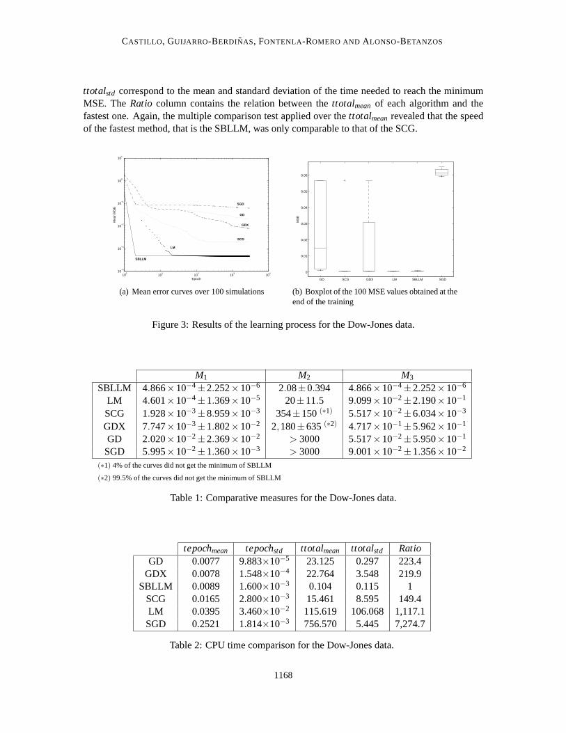
Also, different measures were calculated and collected in Table 4.1. These measures are:

• M1: Mean and standard deviation of the minimum MSEs obtained by each method over the100 simulations.

• M2: Mean epoch and corresponding standard deviation in which each of theother methodsreaches the minimum MSE obtained by the SBLLM.

• M3: MSE and standard deviation for each of the other methods at the epoch in which theSBLLM gets its minimum.

In this case, the best mean MSE is achieved by the LM method (seeM1 in Table 4.1). Also,applying the multiple comparison test, it was found that the difference betweenthis mean and thosefrom the others methods was statistically significant.

Finally, the mean CPU times and the corresponding standard deviations for each of the methodsare shown in Table 4.1. In this table, the variablestepochmean and tepochstd are the mean andstandard deviation CPU time (in seconds) per epoch, respectively, while the variablesttotalmeanand

1167


ttotalstd correspond to the mean and standard deviation of the time needed to reach theminimumMSE. TheRatio column contains the relation between thettotalmean of each algorithm and thefastest one. Again, the multiple comparison test applied over thettotalmeanrevealed that the speedof the fastest method, that is the SBLLM, was only comparable to that of the SCG.

100

101

102

103

104

10−4

10−3

10−2

10−1

100

101

Epoch

Mea

n M

SE

SBLLM

LM

SGD

SCG

GDX

GD

(a) Mean error curves over 100 simulations

GD SCG GDX LM SBLLM SGD

0

0.01

0.02

0.03

0.04

0.05

0.06

MS

E(b) Boxplot of the 100 MSE values obtained at theend of the training

Figure 3: Results of the learning process for the Dow-Jones data.

M1 M2 M3

SBLLM 4.866×10−4±2.252×10−6 2.08±0.394 4.866×10−4±2.252×10−6

LM 4.601×10−4±1.369×10−5 20±11.5 9.099×10−2±2.190×10−1

SCG 1.928×10−3±8.959×10−3 354±150(∗1) 5.517×10−2±6.034×10−3

GDX 7.747×10−3±1.802×10−2 2,180±635(∗2) 4.717×10−1±5.962×10−1

GD 2.020×10−2±2.369×10−2 > 3000 5.517×10−2±5.950×10−1

SGD 5.995×10−2±1.360×10−3 > 3000 9.001×10−2±1.356×10−2

(∗1) 4% of the curves did not get the minimum of SBLLM

(∗2) 99.5% of the curves did not get the minimum of SBLLM

Table 1: Comparative measures for the Dow-Jones data.

tepochmean tepochstd ttotalmean ttotalstd RatioGD 0.0077 9.883×10−5 23.125 0.297 223.4

GDX 0.0078 1.548×10−4 22.764 3.548 219.9SBLLM 0.0089 1.600×10−3 0.104 0.115 1

SCG 0.0165 2.800×10−3 15.461 8.595 149.4LM 0.0395 3.460×10−2 115.619 106.068 1,117.1SGD 0.2521 1.814×10−3 756.570 5.445 7,274.7

Table 2: CPU time comparison for the Dow-Jones data.

1168


4.2 K.U. Leuven Competition Data

The K.U. Leuven time series prediction competition data (Suykens and Vandewalle, 1998) weregenerated from a computer simulated 5-scroll attractor, resulting from a generalized Chua’s circuitwhich is a paradigm for chaos. 1800 data points of this time series were usedfor training. Theaim of the neural network is to predict the current sample using only 4 previous data points. Thusthe training set is reduced to 1796 input patterns corresponding to the number of 4-samples slidingwindows over the initial training set. For this problem a 4-8-1 topology was used. As for theprevious experiment 100 simulations of 3000 iterations each were carried out. Results are shown inFigure 4, and Tables 4.2 and 4.2.

In this case, the best mean MSE is achieved by the LM method (seeM1 in Table 4.2). However,the multiple comparison test did not show any significant difference with respect to the means ofthe SCG and the SBLLM. Regarding thettotalmean, the multiple comparison test showed that thespeed of the fastest method, that is the SBLLM, was only comparable to thoseof the GDX and theGD.

100

101

102

103

104

10−5

10−4

10−3

10−2

10−1

100

101

Epoch

Mea

n M

SE

SBLLM

LM

SGD

SCG

GDX GD


GD SCG GDX LM SBLLM SGD

10−4

10−3

MS

E

(b) Boxplot of the 100 MSE values obtained at theend of the training

Figure 4: Results of the learning process for the Leuven competition data.

M1 M2 M3

SBLLM 3.639×10−5±2.098×10−7 2.2±0.471 3.639×10−5±2.098×10−7

LM 2.7064×10−5±2.439×10−6 23.5±16.3 1.323×10−1±3.143×10−1

SCG 3.517×10−5±9.549×10−7 2160±445(∗) 1.949×10−1±2.083×10−1

GDX 8.121×10−4±4.504×10−4 > 3000 7.190×10−1±6.651×10−1

GD 3.280×10−3±1.698×10−3 > 3000 1.949×10−1±6.621×10−1

SGD 4.748×10−5±9.397×10−6 > 3000 8.458×10−3±5.292×10−3

(∗) 9.8% of the curves did not get the minimum of SBLLM

Table 3: Comparative measures for the Leuven competition data.

1169


tepochmean tepochstd ttotalmean ttotalstd RatioGDX 0.0114 3.256×10−4 34.309 0.977 710.3GD 0.0117 3.208×10−4 35.018 0.963 725

SBLLM 0.0173 2.362×10−3 0.048 0.017 1SCG 0.0238 6.271×10−4 69.571 5.022 1440.4LM 0.0669 5.440×10−2 196.816 164.539 4074.9SGD 0.5083 2.982×10−3 1,525.34 8.949 31,777.9

Table 4: CPU time comparison for the Leuven competition data.

4.3 Lorenz Time Series

A Lorenz system (Lorenz, 1963) is described by the solution of three simultaneous differentialequations:

dx/dt = −σx+σy

dy/dt = −xz+ rx−y

dz/dt = xy−bz,

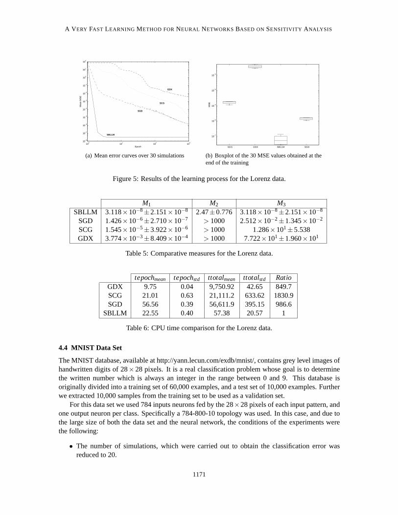
whereσ, r andb are constants. For this work, we employedσ = 10, r = 28, andb = 8/3, for whichthe system presents a chaotic dynamics. The goal of the network is to predict the current samplebased on the four previous samples. For this data set a 8-100-1 topologywas used. Also, 150000samples were employed for the learning process. In this case, and due to the large size of both thedata set and the neural networks, the conditions of the experiments were the following:

• The number of simulations, which were carried out to obtain the MSE curves during thelearning process was reduced to 30, of 1000 iterations each.

• Neither the GD nor the LM methods were used. The results of the GD will not bepresentedbecause the method performed poorly, and the LM is impractical in these cases as it is highlycomputationally demanding (LeCun et al., 1998).

Results are shown in Figure 5, and Tables 4.3 and 4.3. In this case, the SBLLM was the bestboth in mean MSE and total CPU time, confirmed by the multiple comparison test.

1170


100

101

102

103

10−8

10−7

10−6

10−5

10−4

10−3

10−2

10−1

100

101

102

Epoch

Mea

n M

SE

SBLLM

SGD

SCG

GDX


SCG GDX SBLLM SGD

10−7

10−6

10−5

10−4

10−3

MS

E

(b) Boxplot of the 30 MSE values obtained at theend of the training

Figure 5: Results of the learning process for the Lorenz data.

M1 M2 M3

SBLLM 3.118×10−8±2.151×10−8 2.47±0.776 3.118×10−8±2.151×10−8

SGD 1.426×10−6±2.710×10−7 > 1000 2.512×10−2±1.345×10−2

SCG 1.545×10−5±3.922×10−6 > 1000 1.286×101±5.538GDX 3.774×10−3±8.409×10−4 > 1000 7.722×101±1.960×101

Table 5: Comparative measures for the Lorenz data.

tepochmean tepochstd ttotalmean ttotalstd RatioGDX 9.75 0.04 9,750.92 42.65 849.7SCG 21.01 0.63 21,111.2 633.62 1830.9SGD 56.56 0.39 56,611.9 395.15 986.6

SBLLM 22.55 0.40 57.38 20.57 1

Table 6: CPU time comparison for the Lorenz data.

4.4 MNIST Data Set

The MNIST database, available at http://yann.lecun.com/exdb/mnist/, contains grey level images ofhandwritten digits of 28×28 pixels. It is a real classification problem whose goal is to determinethe written number which is always an integer in the range between 0 and 9. This database isoriginally divided into a training set of 60,000 examples, and a test set of 10,000 examples. Furtherwe extracted 10,000 samples from the training set to be used as a validation set.

For this data set we used 784 inputs neurons fed by the 28×28 pixels of each input pattern, andone output neuron per class. Specifically a 784-800-10 topology was used. In this case, and due tothe large size of both the data set and the neural network, the conditions ofthe experiments werethe following:

• The number of simulations, which were carried out to obtain the classification error wasreduced to 20.

1171


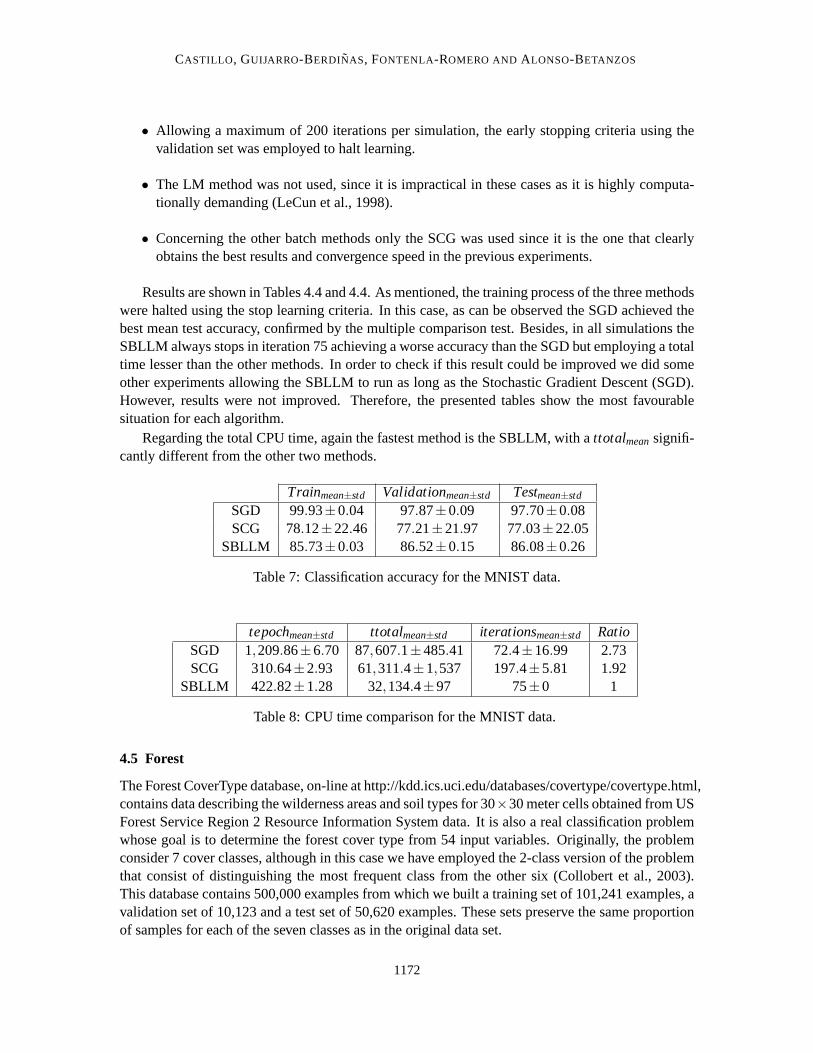
• Allowing a maximum of 200 iterations per simulation, the early stopping criteria usingthevalidation set was employed to halt learning.

• The LM method was not used, since it is impractical in these cases as it is highlycomputa-tionally demanding (LeCun et al., 1998).

• Concerning the other batch methods only the SCG was used since it is the one that clearlyobtains the best results and convergence speed in the previous experiments.

Results are shown in Tables 4.4 and 4.4. As mentioned, the training process of the three methodswere halted using the stop learning criteria. In this case, as can be observed the SGD achieved thebest mean test accuracy, confirmed by the multiple comparison test. Besides,in all simulations theSBLLM always stops in iteration 75 achieving a worse accuracy than the SGD but employing a totaltime lesser than the other methods. In order to check if this result could be improved we did someother experiments allowing the SBLLM to run as long as the Stochastic GradientDescent (SGD).However, results were not improved. Therefore, the presented tablesshow the most favourablesituation for each algorithm.

Regarding the total CPU time, again the fastest method is the SBLLM, with attotalmeansignifi-cantly different from the other two methods.

Trainmean±std Validationmean±std Testmean±std

SGD 99.93±0.04 97.87±0.09 97.70±0.08SCG 78.12±22.46 77.21±21.97 77.03±22.05

SBLLM 85.73±0.03 86.52±0.15 86.08±0.26

Table 7: Classification accuracy for the MNIST data.

tepochmean±std ttotalmean±std iterationsmean±std RatioSGD 1,209.86±6.70 87,607.1±485.41 72.4±16.99 2.73SCG 310.64±2.93 61,311.4±1,537 197.4±5.81 1.92

SBLLM 422.82±1.28 32,134.4±97 75±0 1

Table 8: CPU time comparison for the MNIST data.

4.5 Forest

The Forest CoverType database, on-line at http://kdd.ics.uci.edu/databases/covertype/covertype.html,contains data describing the wilderness areas and soil types for 30×30 meter cells obtained from USForest Service Region 2 Resource Information System data. It is also a real classification problemwhose goal is to determine the forest cover type from 54 input variables.Originally, the problemconsider 7 cover classes, although in this case we have employed the 2-class version of the problemthat consist of distinguishing the most frequent class from the other six (Collobert et al., 2003).This database contains 500,000 examples from which we built a training set of 101,241 examples, avalidation set of 10,123 and a test set of 50,620 examples. These sets preserve the same proportionof samples for each of the seven classes as in the original data set.

1172


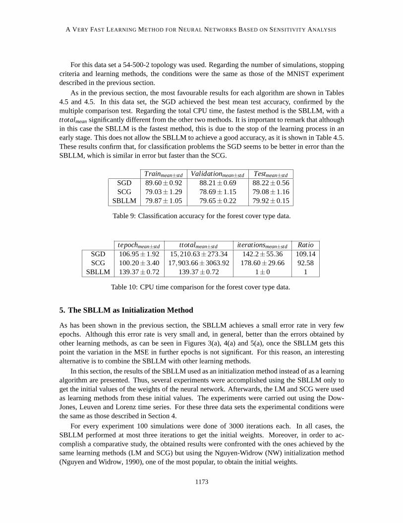
For this data set a 54-500-2 topology was used. Regarding the number ofsimulations, stoppingcriteria and learning methods, the conditions were the same as those of the MNIST experimentdescribed in the previous section.

As in the previous section, the most favourable results for each algorithm are shown in Tables4.5 and 4.5. In this data set, the SGD achieved the best mean test accuracy,confirmed by themultiple comparison test. Regarding the total CPU time, the fastest method is the SBLLM, with attotalmeansignificantly different from the other two methods. It is important to remark that althoughin this case the SBLLM is the fastest method, this is due to the stop of the learning process in anearly stage. This does not allow the SBLLM to achieve a good accuracy, as it is shown in Table 4.5.These results confirm that, for classification problems the SGD seems to be better in error than theSBLLM, which is similar in error but faster than the SCG.

Trainmean±std Validationmean±std Testmean±std

SGD 89.60±0.92 88.21±0.69 88.22±0.56SCG 79.03±1.29 78.69±1.15 79.08±1.16

SBLLM 79.87±1.05 79.65±0.22 79.92±0.15

Table 9: Classification accuracy for the forest cover type data.

tepochmean±std ttotalmean±std iterationsmean±std RatioSGD 106.95±1.92 15,210.63±273.34 142.2±55.36 109.14SCG 100.20±3.40 17,903.66±3063.92 178.60±29.66 92.58

SBLLM 139.37±0.72 139.37±0.72 1±0 1

Table 10: CPU time comparison for the forest cover type data.

5. The SBLLM as Initialization Method

As has been shown in the previous section, the SBLLM achieves a small error rate in very fewepochs. Although this error rate is very small and, in general, better than the errors obtained byother learning methods, as can be seen in Figures 3(a), 4(a) and 5(a),once the SBLLM gets thispoint the variation in the MSE in further epochs is not significant. For this reason, an interestingalternative is to combine the SBLLM with other learning methods.

In this section, the results of the SBLLM used as an initialization method instead of as a learningalgorithm are presented. Thus, several experiments were accomplishedusing the SBLLM only toget the initial values of the weights of the neural network. Afterwards, theLM and SCG were usedas learning methods from these initial values. The experiments were carriedout using the Dow-Jones, Leuven and Lorenz time series. For these three data sets the experimental conditions werethe same as those described in Section 4.

For every experiment 100 simulations were done of 3000 iterations each. In all cases, theSBLLM performed at most three iterations to get the initial weights. Moreover, in order to ac-complish a comparative study, the obtained results were confronted with the ones achieved by thesame learning methods (LM and SCG) but using the Nguyen-Widrow (NW) initialization method(Nguyen and Widrow, 1990), one of the most popular, to obtain the initial weights.

1173


Figures 6(a), 7(a) and 8(a) show the corresponding mean curves (over the 100 simulations) ofthe learning process using the SBLLM and the NW as initialization methods and theLM as thelearning algorithm. Figures 6(b), 7(b) and 8(b) show the same mean curves of the learning processusing this time the SCG as learning algorithm.

100

101

102

103

104

10−4

10−3

10−2

10−1

100

101

Epoch

Mea

n M

SE

NW + LM

SBLLM + LM

(a) Mean error curves for the LM method

100

101

102

103

104

10−4

10−3

10−2

10−1

100

101

Epoch

Mea

n M

SE

NW + SCG

SBLLM + SCG

(b) Mean error curves for the SCG method

Figure 6: Mean error curves over 100 simulations for the Dow-Jones time series using the SBLLMand the NW as initialization methods.

100

101

102

103

104

10−5

10−4

10−3

10−2

10−1

100

101

Epoch

Mea

n M

SE

NW + LM

SBLLM + LM


100

101

102

103

104

10−5

10−4

10−3

10−2

10−1

100

101

Epoch

Mea

n M

SE

NW + SCG

SBLLM + SCG


Figure 7: Mean error curves over 100 simulations for the Leuven competition time series using theSBLLM and the NW as initialization methods.

1174


100

101

102

103

104

10−14

10−12

10−10

10−8

10−6

10−4

10−2

100

102

Mea

n M

SE

NW + LM

SBLLM + LM

Epoch


100

101

102

103

104

10−10

10−8

10−6

10−4

10−2

100

102

Epoch

Mea

n M

SE

NW + SCG

SBLLM + SCG


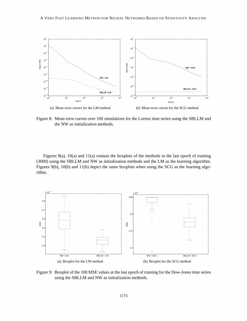
Figure 8: Mean error curves over 100 simulations for the Lorenz time series using the SBLLM andthe NW as initialization methods.

Figures 9(a), 10(a) and 11(a) contain the boxplots of the methods in the last epoch of training(3000) using the SBLLM and NW as initialization methods and the LM as the learning algorithm.Figures 9(b), 10(b) and 11(b) depict the same boxplots when using the SCG as the learning algo-rithm.

NW + LM SBLLM + LM

4.3

4.4

4.5

4.6

4.7

4.8

x 10−4

MS

E

(a) Boxplot for the LM method

NW + SCG SBLLM + SCG

4.7

4.75

4.8

4.85

x 10−4

MS

E

(b) Boxplot for the SCG method

Figure 9: Boxplot of the 100 MSE values at the last epoch of training for the Dow-Jones time seriesusing the SBLLM and NW as initialization methods.

1175


NW + LM SBLLM + LM

2.2

2.3

2.4

2.5

2.6

2.7

2.8

2.9

3

3.1

x 10−5

MS

E


NW + SCG SBLLM + SCG3.2

3.4

3.6

3.8

4

4.2

4.4

4.6

x 10−5

MS

E


Figure 10: Boxplot of the 100 MSE values at the last epoch of training forthe Leuven competitiontime series using the SBLLM and NW as initialization methods.

NW + LM SBLLM + LM

0

1

2

3

4

5

6

7

x 10−11

MS

E


NW + SCG SBLLM + SCG

0

0.5

1

1.5

2

2.5

3

3.5

x 10−6

MS

E


Figure 11: Boxplot of the 100 MSE values at the last epoch of training forthe Lorenz time seriesusing the SBLLM and NW as initialization methods.

6. Discussion

Regarding the behavior of the SBLLM as alearning algorithm, and from the experiments made andthe results presented in Section 4, there are three main features of the SBLLM that stand out:

1. High speed in reaching the minimum error. For the first three problems (Dow-Jones, Leuvenand Lorenz time series), this feature can be observed in Figures 3(a), 4(a) and 5(a), and themeasureM2 in Tables 4.1, 4.2 and 4.3, where it can be seen that in all cases the SBLLM

1176


obtains its minimum MSE (minMSE) just before the first 4 iterations and also sooner thanthe rest of the algorithms. Moreover, and generally speaking, measureM3 reflects that theSBLLM gets its minimum in an epoch for which the other algorithms are far from similarMSE values.

If we take into account the CPU times in Tables 4.1, 4.2, 4.3, 4.4 and 4.5 we can see that,as expected, the CPU time per epoch of the SBLLM is similar to that of the SCG (both ofO(n2)), and when we consider the total CPU time per simulation the SBLLM is, in the worstcase, more than 150 times faster than the fastest algorithm for the regression examples andapproximately 2 times faster for the classification examples. It is also important toremarkthat despite of the advantages of the LM method, it could not be applied in the experimentsthat involved large data sets and neural networks as it is impractical for such cases (LeCunet al., 1998).

2. A good performance. From Figures 3(a), 4(a) and 5(a), and the measureM1 in Tables 4.1, 4.2and 4.3, it can be deduced that not only the SBLLM stabilizes soon, but also the minMSE thatit reaches is quite good and comparable to that obtained by the second order methods. On theother hand, the GD and the GDX learning methods never succeeded in attaining this minMSEbefore the maximum number of epochs, as reflected in measureM2 (Tables 4.1, 4.2 and 4.3).Finally, the SCG algorithm presents an intermediate behavior, although seldomachieves thelevels of performance of the LM and SBLLM.

Regarding the classification problems, from Tables 4.4 and 4.5, it can be deduced that theSBLLM performs similar or better than the other batch method, that is the SCG, while thestochastic method (SGD) is the best algorithm for this kind of problems (LeCunet al., 1998).

Although the ability of the proposed algorithm to get a minimum in just very few epochsis usually an advantage, it can also be noticed that once it achieves this minimum(localor global) it gets stuck in this point. This causes that, sometimes like in the classificationexamples included, the algorithm is not able to obtain a high accuracy. This behavior couldbe explained by the initialization method and the updating rule for the step size employed.

3. Homogeneous behavior. This feature comprehends several aspects:

• The SBLLM learning curve stabilizes soon, as can be observed in Figures 3(a), 4(a) and5(a).

• Regarding the minimum MSE reached at the end of the learning process, it can beobserved from Figures 3(b), 4(b) and 5(b) that, in any case, the GD and GDX algorithmspresent a wider dispersion, given even place to the appearance of outliers. On the otherhand, the SGD, SCG, LM and SBLLM algorithms tend to always obtain nearervaluesof MSE. This fact is also reflected by the standard deviations of measureM1.

• The SBLLM behaves homogeneously not only if we consider just the end of the learningprocess, as commented, but also during the whole process, in such a waythat very sim-ilar learning curves where obtained for all iterations of the first three experiments. Thisis, in a certain way, reflected in the standard deviation of measureM3 which correspondsto the MSE value taken at some intermediate point of the learning process.

1177


• Finally, from Tables 4.4 and 4.5 it can be observed that for these last two experiments(MNIST and Forest databases) this homogeneus behaviour stands forthe SGD and theSBLLM, while the SCG presents a wider dispersion in its classification errors.

With respect to the use of the SBLLM asinitialization method, as it can be observed in Figures6, 7 and 8, the SBLLM combined with the LM or the SCG achieves a faster convergence speed thanthe same methods using the NW as initialization method. Also, the SBLLM obtains a very goodinitial point, and thus a very low MSE in a few epochs of training. Moreover,in this case, mostof the times the final MSE achieved is smaller than the one obtained using the NW initializationmethod. This result is better illustrated in the boxplots of the corresponding time series where it canbe observed, in addition, that the final MSE obtained with NW presents a higher variability thanthat achieved by the SBLLM, that is, the SBLLM helps the learning algorithms toobtain a morehomogeneous MSE at the end of the training process. Thus, experiments confirm the utility of theSBLLM as an initialization method, which effect is to speed up the convergence.

7. Conclusions and Future Work

The main conclusions that can be drawn from this paper are:

1. The sensitivities of the sum of squared errors with respect to the outputs of the intermediatelayer allow an efficient and fast gradient method to be applied.

2. Over the experiments made the SBLLM offers an interesting combination of speed, reliabilityand simplicity.

3. Regarding the employed regression problems only second order methods, and more specifi-cally the LM, seem to obtain similar results although at a higher computational cost.

4. With respect to the employed classification problems, the SBLLM performs similar or bet-ter than the other batch method, although requiring less computational time. Besides, thestochastic gradient (SGD) is the one that obtains the lowest classification error. This result isin accordance with that obtained by other authors (LeCun et al., 1998) that recommend thismethod for large data sets and networks in classification tasks.

5. The SBLLM used as an initialization method significantly improves the performance of alearning algorithm.

Finally, there are some aspects of the proposed algorithm that need an in depth study, and willbe addressed in a future work:

1. A more appropriate method to set the initial values of the outputsz of hidden neurons (step 0of the proposed algorithm).

2. A more efficient updating rule for the step sizeρ, like a method based on a line search (hardor soft).

3. An adaptation of the algorithm to improve its performance on classification problems, specif-ically for large data sets.

1178


Acknowledgments

We would like to acknowledge support for this project from the Spanish Ministry of Science andTechnology (Projects DPI2002-04172-C04-02 and TIC2003-00600, this last partially supported byFEDER funds) and the Xunta de Galicia (project PGIDT04PXIC10502PN). Also, we thank theSupercomputing Center of Galicia (CESGA) for allowing us the use of the highperformance com-puting servers.

References

L. B. Almeida, T. Langlois, J. D. Amaral, and A. Plakhov. Parameter adaptation in stochasticoptimization. In D. Saad, editor,On-line Learning in Neural Networks, chapter 6, pages 111–134. Cambridge University Press, 1999.

R. Battiti. First and second order methods for learning: Between steepestdescent and Newton’smethod.Neural Computation, 4(2):141–166, 1992.

E. M. L. Beale. A derivation of conjugate gradients. In F. A. Lootsma, editor, Numerical methodsfor nonlinear optimization, pages 39–43. Academic Press, London, 1972.

F. Biegler-Konig and F. Barmann. A learning algorithm for multilayered neural networks based onlinear least-squares problems.Neural Networks, 6:127–131, 1993.

W. L. Buntine and A. S. Weigend. Computing second derivatives in feed-forward networks: Areview. IEEE Transactions on Neural Networks, 5(3):480–488, 1993.

E. Castillo, J. M. Gutierrez, and A. Hadi. Sensitivity analysis in discrete bayesian networks.IEEETransactions on Systems, Man and Cybernetics, 26(7):412–423, 1997.

E. Castillo, A. Cobo, J. M. Gutierrez, and R. E. Pruneda. Working with differential, functional anddifference equations using functional networks.Applied Mathematical Modelling, 23(2):89–107,1999.

E. Castillo, A. Cobo, J. M. Gutierrez, and R. E. Pruneda. Functional networks. a new neural networkbased methodology.Computer-Aided Civil and Infrastructure Engineering, 15(2):90–106, 2000.

E. Castillo, A. Conejo, P. Pedregal, R. Garcıa, and N. Alguacil.Building and Solving MathematicalProgramming Models in Engineering and Science. John Wiley & Sons Inc., New York., 2001.

E. Castillo, O. Fontenla-Romero, A. Alonso Betanzos, and B. Guijarro-Berdinas. A global optimumapproach for one-layer neural networks.Neural Computation, 14(6):1429–1449, 2002.

E. Castillo, A. S. Hadi, A. Conejo, and A. Fernandez-Canteli. A general method for local sensitivityanalysis with application to regression models and other optimization problems.Technometrics,46(4):430–445, 2004.

E. Castillo, C. Castillo A. Conejo and, R. Mınguez, and D. Ortigosa. A perturbation approach tosensitivity analysis in nonlinear programming.Journal of Optimization Theory and Applications,128(1):49–74, 2006.

1179


A. Chella, A. Gentile, F. Sorbello, and A. Tarantino. Supervised learningfor feed-forward neuralnetworks: a new minimax approach for fast convergence.Proceedings of the IEEE InternationalConference on Neural Networks, 1:605 – 609, 1993.

V. Cherkassky and F. Mulier.Learning from Data: Concepts, Theory, and Methods. Wiley, NewYork, 1998.

R. Collobert, Y. Bengio, and S. Bengio. Scaling large learning problems withhard parallel mixtures.International Journal of Pattern Recognition and Artificial Intelligence, 17(3):349–365, 2003.

J. E. Dennis and R. B. Schnabel.Numerical Methods for Unconstrained Optimization and NonlinearEquations. Prentice-Hall, Englewood Cliffs, NJ, 1983.

G. P. Drago and S. Ridella. Statistically controlled activation weight initialization (SCAWI). IEEETransactions on Neural Networks, 3:899–905, 1992.

R. Fletcher and C. M. Reeves. Function minimization by conjugate gradients.Computer Journal, 7(149–154), 1964.

O. Fontenla-Romero, D. Erdogmus, J.C. Principe, A. Alonso-Betanzos,and E. Castillo. Linearleast-squares based methods for neural networks learning.Lecture Notes in Computer Science,2714(84–91), 2003.

M. T. Hagan and M. Menhaj. Training feedforward networks with the marquardt algorithm.IEEETransactions on Neural Networks, 5(6):989–993, 1994.

M. T. Hagan, H. B. Demuth, and M. H. Beale.Neural Network Design. PWS Publishing, Boston,MA, 1996.

M. Hollander and D. A. Wolfe.Nonparametric Statistical Methods. John Wiley & Sons, 1973.

J. C. Hsu. Multiple Comparisons. Theory and Methods. Chapman&Hall/CRC, Boca Raton, FL,1996.

D. R. Hush and J. M. Salas. Improving the learning rate of back-propagation with the gradient reusealgorithm.Proceedings of the IEEE Conference of Neural Networks, 1:441–447, 1988.

B. C. Ihm and D. J. Park. Acceleration of learning speed in neural networks by reducing weightoscillations. Proceedings of the International Joint Conference on Neural Networks, 3:1729–1732, 1999.

R. A. Jacobs. Increased rates of convergence through learning rate adaptation.Neural Networks, 1(4):295–308, 1988.

Y. LeCun, I. Kanter, and S.A. Solla. Second order properties of error surfaces: Learning time andgeneralization. In R.P. Lippmann, J.E. Moody, and D.S. Touretzky, editors, Neural InformationProcessing Systems, volume 3, pages 918–924, San Mateo, CA, 1991. Morgan Kaufmann.

Y. LeCun, L. Bottou, G.B. Orr, and K.-R. Muller. Efficient backprop. In G. B. Orr and K.-R. Muller,editors,Neural Networks: Tricks of the trade, number 1524 in LNCS. Springer-Verlag, 1998.

1180


K. Levenberg. A method for the solution of certain non-linear problems in least squares.QuaterlyJournal of Applied Mathematics, 2(2):164–168, 1944.

E. Ley. On the peculiar distribution of the U.S. stock indeces’ first digits.The American Statistician,50(4):311–314, 1996.

E. N. Lorenz. Deterministic nonperiodic flow.Journal of the Atmospheric Sciences, 20:130–141,1963.

D. W. Marquardt. An algorithm for least-squares estimation of non-linear parameters.Journal ofthe Society of Industrial and Applied Mathematics, 11(2):431–441, 1963.

M. F. Moller. A scaled conjugate gradient algorithm for fast supervisedlearning.Neural Networks,6:525–533, 1993.

D. Nguyen and B. Widrow. Improving the learning speed of 2-layer neural networks by choosinginitial values of the adaptive weights.Proceedings of the International Joint Conference onNeural Networks, 3:21–26, 1990.

G. B. Orr and T. K. Leen. Using curvature information for fast stochastic search. In M.I. Jordan,M.C. Mozer, and T. Petsche, editors,Neural Information Processing Systems, volume 9, pages606–612, Cambridge, 1996. MIT Press.

D. B. Parker. Optimal algorithms for adaptive networks: second order back propagation, secondorder direct propagation, and second order hebbian learning.Proceedings of the IEEE Conferenceon Neural Networks, 2:593–600, 1987.

S. Pethel, C. Bowden, and M. Scalora. Characterization of optical instabilities and chaos using MLPtraining algorithms.SPIE Chaos Opt., 2039:129–140, 1993.

M. J. D. Powell. Restart procedures for the conjugate gradient method.Mathematical Programming,12:241–254, 1977.

S. Ridella, S. Rovetta, and R. Zunino. Circular backpropagation networks for classification.IEEETransactions on Neural Networks, 8(1):84–97, January 1997.

A. K. Rigler, J. M. Irvine, and T. P. Vogl. Rescaling of variables in backpropagation learning.Neural Networks, 4:225–229, 1991.

D. E. Rumelhart, G. E. Hinton, and R. J. Willian. Learning representations of back-propagationerrors.Nature, 323:533–536, 1986.

N. N. Schraudolph. Fast curvature matrix-vector products for second order gradient descent.NeuralComputation, 14(7):1723–1738, 2002.

A. Sperduti and S. Antonina. Speed up learning and network optimization withextended backpropagation.Neural Networks, 6:365–383, 1993.

J. A. K. Suykens and J. Vandewalle, editors.Nonlinear Modeling: advanced black-box techniques.Kluwer Academic Publishers Boston, 1998.

1181


T. Tollenaere. Supersab: Fast adaptive back propagation with good scaling properties.NeuralNetworks, 3(561–573), 1990.

T. P. Vogl, J. K. Mangis, A. K. Rigler, W. T. Zink, and D. L. Alkon. Accelerating the convergenceof back-propagation method.Biological Cybernetics, 59:257–263, 1988.

M. K. Weir. A method for self-determination of adaptive learning rates in back propagation.NeuralNetworks, 4:371–379, 1991.

B. M. Wilamowski, S. Iplikci, O. Kaynak, and M. O. Efe. An algorithm for fast convergence intraining neural networks.Proceedings of the International Joint Conference on Neural Networks,2:1778–1782, 2001.

J. Y. F. Yam, T. W. S Chow, and C. T Leung. A new method in determining the initial weights offeedforward neural networks.Neurocomputing, 16(1):23–32, 1997.

1182

A Very Fast Learning Method for Neural Networks Based on ...

Documents

Transcript of A Very Fast Learning Method for Neural Networks Based on ...