A VERTEX-BASED HIGH-ORDER FINITE-VOLUME...

11th World Congress on Computational Mechanics (WCCM XI)5th European Conference on Computational Mechanics (ECCM V)

6th European Conference on Computational Fluid Dynamics (ECFD VI)E. Onate, J. Oliver and A. Huerta (Eds)

A VERTEX-BASED HIGH-ORDER FINITE-VOLUMESCHEME FOR THREE-DIMENSIONAL COMPRESSIBLE

FLOWS ON TETRAHEDRAL MESH

MARC R.J. CHAREST1, THOMAS R. CANFIELD2,NATHANIEL R. MORGAN3, JACOB WALTZ4,

AND JOHN G. WOHLBIER5

1 Los Alamos National Laboratory, Los Alamos, NM, U.S.A., [email protected] Los Alamos National Laboratory, Los Alamos, NM, U.S.A., [email protected] Los Alamos National Laboratory, Los Alamos, NM, U.S.A., [email protected] Los Alamos National Laboratory, Los Alamos, NM, U.S.A., [email protected]

5 Los Alamos National Laboratory, Los Alamos, NM, U.S.A., [email protected]

Key words: Numerical Algorithms, Computational Fluid Dynamics, High-Order Meth-ods, Compressible Flows, Shock Hydrodynamics.

Abstract. High-order discretization methods offer the potential to reduce the compu-tational cost associated with modelling compressible flows. However, it is difficult toobtain accurate high-order discretizations of conservation laws that do not produce spuri-ous oscillations near discontinuities, especially on multi-dimensional unstructured mesh.To overcome this issue, a novel, high-order, central essentially non-oscillatory (CENO)finite-volume method was proposed for tetrahedral mesh. The proposed unstructuredmethod is vertex-based, which differs from existing cell-based CENO formulations, anduses a hybrid reconstruction procedure that switches between two different solution repre-sentations. It applies a high-order k-exact reconstruction in smooth regions and a limitedlinear one when discontinuities are encountered. Both reconstructions use a single, cen-tral stencil for all variables, making the application of CENO to arbitrary unstructuredmeshes relatively straightforward. The new approach was applied to the conservationequations governing compressible flows and assessed in terms of accuracy and computa-tional cost. For all problems considered, which included various function reconstructionsand idealized flows, CENO demonstrated excellent reliability and robustness. High-orderaccuracy was achieved in smooth regions and essentially non-oscillatory solutions wereobtained near discontinuities. The high-order schemes were also more computationallyefficient for high-accuracy solutions, i.e., they took less wall time than the lower-orderschemes to achieve a desired level of error.

LANL report no. LA-UR-14-22349

1

M.R.J. Charest, T.R. Canfield, N.R. Morgan, J. Waltz and J.G. Wohlbier

1 INTRODUCTION

Finite-volume methods are a popular discretization technique for computational fluiddynamics, especially for compressible flows. Numerous formulations exist, and one of themain differing characteristics is the approach used to discretize the computational domain.Either cell- or vertex-based discretizations are typically employed. Cell-based approachesapply conservation laws to the individual elements or cells of the mesh, whereas vertex-based approaches apply them to control volumes constructed surrounding the verticesof the mesh. The choice is not always straightforward, since both techniques are widelyused and both have their respective advantages/disadvantages. For example, vertex-basedschemes are often favored for use with unstructured tetrahedral mesh since there is approx-imately 5 to 6 times fewer vertices than elements. But because there are more elementsthan vertices in a tetrahedral mesh, cell-based schemes have more degrees of freedom. Assuch, cell-based schemes tend to be slightly more accurate on tetrahedral meshes, althoughthis increased accuracy comes at the expense of additional computational effort [1]. Thedirect comparison between the two types of schemes is complicated, however, becausethey both use different stencils. The larger, denser stencils that vertex-based schemesare more robust and accurate per degree of freedom, which may make vertex centeredschemes more computationally efficient for a given accuracy [1]. Nonetheless, whateverthe chosen finite-volume formulation, current production codes rely mostly on standardfirst- or second-order accurate discretization schemes. These discretizations are often notpractical for physically-complex, multi-dimensional flows with disparate scales as theytend to exhibit excessive numerical dissipation.

High-order discretization methods for conservation laws have the potential to signif-icantly reduce the cost of modelling physically-complex flows. They offer improved nu-merical efficiency to obtain high-resolution solutions since fewer computational cells arerequired to achieve a desired level of accuracy [2]. However, this potential is challengingto fully realize as it is difficult to obtain accurate and robust discretizations of hyperbolicconservation laws near discontinuities [3]. Although there are many different high-orderschemes for both structured and unstructured mesh that attempt to address this issue [3–31], there is still no consensus on a robust, efficient, and accurate scheme that deals withthe aforementioned issues and is universally applicable to arbitrary meshes.

One promising high-order discretization is the central essentially non oscillatory (CENO)finite-volume approach [32–40]. It was originally developed for two-dimensional structuredmesh by Ivan et al. [36–40] and then extended to three-dimensional unstructured meshby Charest et al. [32–35]. In all formulations, CENO remained both accurate and robustthroughout a variety of physically-complex flows. This robustness is provided by a hybridreconstruction procedure that switches between two algorithms: an unlimited high-orderk-exact reconstruction in smooth regions, and a monotonicity-preserving limited piecewiselinear reconstruction in regions with discontinuities or shocks. Switching between the tworeconstructions is facilitated by a smoothness indicator that measures the ability of the

2


of the k-exact reconstruction to locally resolve the flow. Fixed central stencils are usedfor both reconstruction algorithms, which makes its extension to arbitrary unstructuredmeshes straightforward.

The CENO approach avoids many of the complexities associated with other essentiallynon-oscillatory (ENO) [3] and weighted ENO (WENO) [8, 10, 11] finite-volume schemesbecause it does not require a high-order reconstruction on multiple stencils. Both ENOand WENO schemes have difficulty selecting stencils on general multi-dimensional un-structured meshes [5, 6, 9, 41], and some of these stencils produce poorly conditionedlinear systems for solution reconstruction [9, 41].

The existing CENO formulations for structured [36–40] and unstructured [32–35] mesheswere developed for cell-based finite-volume schemes only. In the present research, CENOwas extended to a vertex-based finite-volume discretization for three-dimensional unstruc-tured mesh and applied to solve the equations governing compressible flows. The resultingalgorithm was applied to various function reconstructions, as well as steady and unsteadyflows, and then analyzed with respect to accuracy and computational cost. This researchwas performed using Chicoma, a computational framework for compressible fluid flow,i.e., shock hydrodynamics [42]

2 GOVERNING EQUATIONS

The Euler equations governing compressible fluid flow were considered for the presentresearch. In three space dimensions, these partial-differential equations (PDEs) are givenby

∂

∂tU(W) + ~∇ · ~F(W) = S(W) (1)

where t is the time, U and W are the vectors of conserved and primitive variables,respectively, ~F(W) = [E,F,G] is the inviscid solution flux dyad, and S(W) is a vectorof source terms. These terms are defined as

U =[ρ, ρu, ρv, ρw, ρet

],

W =[ρ, u, v, w, e

],

E =

ρu

ρu2 + pρuvρuw

u(ρet + p)

, F =

ρvρvu

ρv2 + pρvw

v(ρet + p)

, G =

ρwρwuρwv

ρw2 + pw(ρet + p)

where ρ is the fluid density, p is the pressure, ~v = (u, v, w) is the fluid velocity vector, e isthe internal energy, and et is the total energy. The total energy is the sum of the internaland kinetic energies, i.e.,

et = e+1

2(u2 + v2 + w2) (2)

3


Ωi

n

Element CentroidEdge Midpoint

Primal Mesh, T (Ω)

Dual Mesh, D(Ω)

Vertex

(a) Primal and dual mesh (shown in two-dimensionsfor simplicity).

(b) Example of a three-dimensional control volume.

Figure 1: Computational mesh and local control volume configuration.

Internal energy is related to pressure and density through the following relation for anideal gas:

e =p

ρ(γ − 1)(3)

where γ is the ratio of specific heats. The sound speed of an ideal gas is given by

a =√γp/ρ (4)

Although Eqs. (3) and (4) describe an ideal gas, the numerical formulation describedherein is designed to support arbitrary analytic or tabular equations of state. Unlessotherwise specified, γ = 1.4.

The source term vector, S, is typically treated as zero throughout this work. There isone particular case — which will be discussed in the following sections — where it wasused to generate a known solution for validation purposes.

3 CENO FINITE-VOLUME SCHEME

In the proposed vertex-based finite-volume approach, the physical domain, Ω, wasdiscretized into non-overlapping, finite-sized control volumes, Ωi, such that

Ω = ∪Ωi (5)

Ωi ∩ Ωj for i 6= j (6)

The individual control volumes were formed by constructing the median dual, D(Ω),of a three-dimensional triangulation of the domain, T (Ω), which is illustrated in two-dimensions in Fig. 1a. Only primal meshes composed of tetrahedral elements were con-sidered, and they have a corresponding dual mesh composed of complex polyhedrons with

4


Table 1: Gauss quadrature rules used for integrating over triangles and tetrahedrons.

Reconstruction Number of Points Degree of Precision

Triangle Tetrahedron

Constant (k=0) 1 1 1

Linear (k=1) 1 1 1

Quadratic (k=2) 3 4 2

Cubic (k=3) 4 8 3

Quartic (k=4) 6 14 4

triangular faces. A control volume surrounding a vertex i, Ωi, was constructed from thepolyhedron whose vertices are the centroids of incident tetrahedra and triangles, plus themidpoints of incident edges. A sample control volume surrounding an individual vertexin a three-dimensional tetrahedral mesh is illustrated in Fig. 1b.

Equation (1) was integrated over each individual control volume to give the followingsystem of ordinary differential equations (ODEs) for control-volume-averaged solutionquantities, Ui:

dUi

dt= − 1

Vi

∮∂Ωi

(~F · n

)dΓ +

1

Vi

∫Ωi

S dΩ = Ri, i = 1, 2, . . . , Nv (7)

where Nv is the number of control volumes (i.e., vertices of the primal mesh), Vi is thevolume and n is the unit vector normal to the surface of the control volume, ∂Ωi. ApplyingGauss quadrature to evaluate the surface and volume integrals in Eq. (7) produces a setof nonlinear ODEs given by

dUi

dt= − 1

Vi

Nf∑j=1

Gf∑k=1

[ωf~F · n

]i,j,k

+1

Vi

Gv∑m=1

[ωv S]i,m = Ri (8)

where Nf is the number of faces, Gf and Gv are the number of quadrature points andωf and ωv are the corresponding quadrature weights for the face and volume integrals,respectively.

In Eq. (8), the number of quadrature points required for each rule is a direct functionof the number of spatial dimensions and the reconstruction order — i.e., the quadraturerule must be able to integrate a k-degree polynomial exactly (k-exactness). Integratingover the individual faces of the polyhedral-shaped control volume is relatively straightfor-ward. Since the faces are triangular, standard quadrature rules for triangles were used.However, general quadrature rules for integrating over complex polyhedrons do not exist.As such, numerical integrals over the volume of these complex elements were evaluated bysubdividing the polyhedrons into tetrahedrons and applying standard Gauss quadrature

5


rules to each individual tetrahedron. The coefficients for the quadrature rules appliedherein are as given by Felippa [43] and summarized in Table 1.

3.1 CENO Reconstruction

Evaluating Eq. (8) requires numerically integrating the fluxes and source terms overthe control-volumes, and this numerical integration requires interpolating the solution atquadrature points. Only control-volume averages are known in the proposed finite-volumeapproach, so the solution at these quadrature points was interpolated using the high-order CENO method [32–40]. The reconstruction was applied to the primitive solutionquantities, W, to ensure that both pressure and internal energy remain positive.

3.1.1 k-Exact Reconstruction

The CENO spatial discretization scheme is based on the high-order k-exact least-squares reconstruction technique of Barth [4, 44]. The k-exact reconstruction algorithmbegins by assuming that the solution within each control-volume is represented by piece-wise Taylor polynomials. In three space dimensions, the polynomials are defined as

uki (x, y, z) =

p+q+r≤k∑p=0

∑q=0

∑r=0

(x− xi)p(y − yi)q(z − zi)rDpqr (9)

where uki is the reconstructed solution quantity, (xi, yi, zi) is the geometric referencepoint, k is the degree of the piecewise polynomial interpolant, and Dpqr are the unknowncoefficients of the Taylor series expansion. Any geometric reference point can be chosen;the vertex about which the control volume is constructed was used here.

The following conditions were applied to determine the unknown coefficients: (i) themean or average value within the computational volume must be preserved; (ii) the solu-tion reconstruction must reproduce polynomials of degree ≤ k exactly (i.e., k-exactness);and (iii) the reconstruction must have compact support. The first condition introduces aconstraint on the reconstruction which states that

ui =1

Vi

∫Ωi

uki (x, y, z) dΩ (10)

where ui is the control-volume average in Ωi. Additional constraints are introduced bythe second condition, requiring that

uki (x, y, z) = uexact +O(hk+1) (11)

in the vicinity of Ωi. The length scale, h, is defined as the maximum diameter of thecontrol-volume circumspheres in the vicinity of Ωi. From Eq. (11), the reconstructionpolynomial for Ωi must also recover the averages of neighboring control volumes. That is,

uj =1

Vj

∫Ωj

uki (x, y, z) dΩ +O(hk+1) ∀j ∈ Sneigh,i (12)

6


1st neighbor

2nd neighbor

Ωi

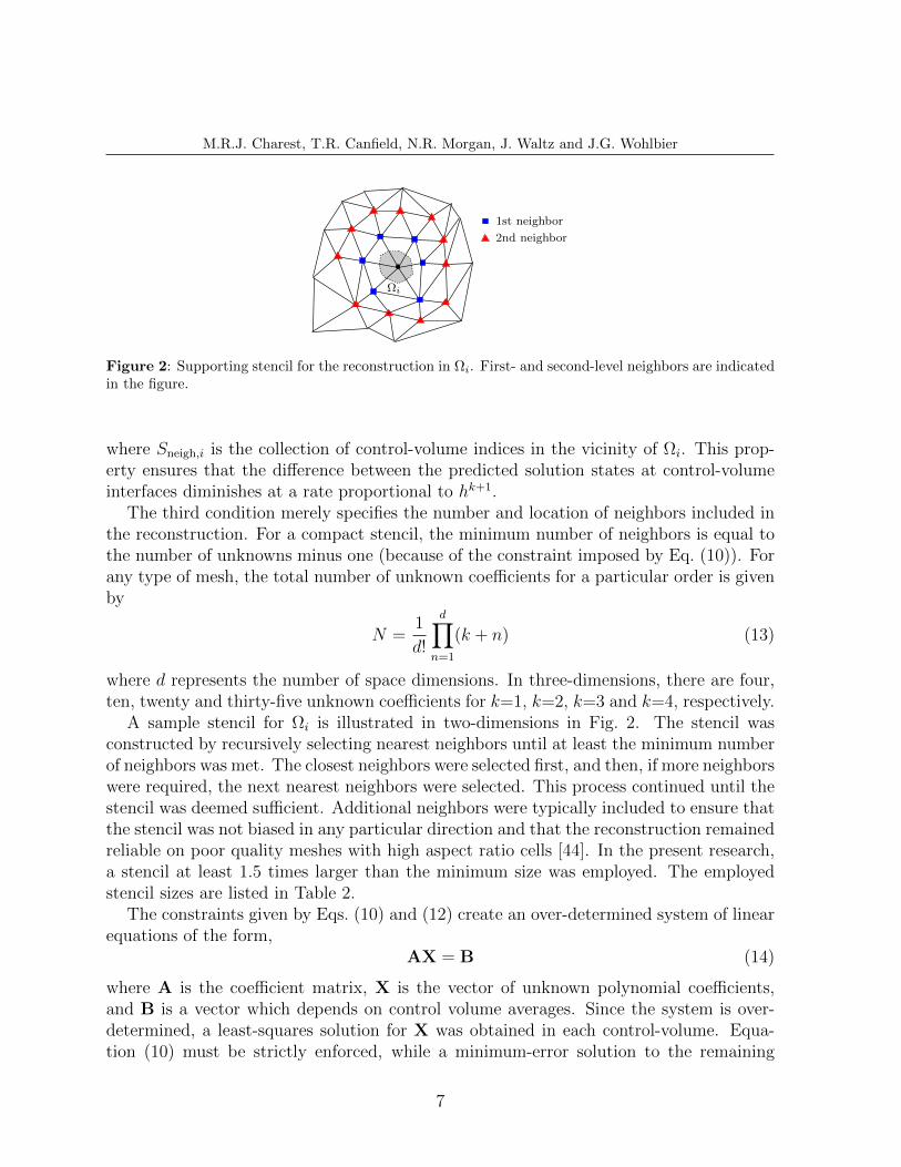
Figure 2: Supporting stencil for the reconstruction in Ωi. First- and second-level neighbors are indicatedin the figure.

where Sneigh,i is the collection of control-volume indices in the vicinity of Ωi. This prop-erty ensures that the difference between the predicted solution states at control-volumeinterfaces diminishes at a rate proportional to hk+1.

The third condition merely specifies the number and location of neighbors included inthe reconstruction. For a compact stencil, the minimum number of neighbors is equal tothe number of unknowns minus one (because of the constraint imposed by Eq. (10)). Forany type of mesh, the total number of unknown coefficients for a particular order is givenby

N =1

d!

d∏n=1

(k + n) (13)

where d represents the number of space dimensions. In three-dimensions, there are four,ten, twenty and thirty-five unknown coefficients for k=1, k=2, k=3 and k=4, respectively.

A sample stencil for Ωi is illustrated in two-dimensions in Fig. 2. The stencil wasconstructed by recursively selecting nearest neighbors until at least the minimum numberof neighbors was met. The closest neighbors were selected first, and then, if more neighborswere required, the next nearest neighbors were selected. This process continued until thestencil was deemed sufficient. Additional neighbors were typically included to ensure thatthe stencil was not biased in any particular direction and that the reconstruction remainedreliable on poor quality meshes with high aspect ratio cells [44]. In the present research,a stencil at least 1.5 times larger than the minimum size was employed. The employedstencil sizes are listed in Table 2.

The constraints given by Eqs. (10) and (12) create an over-determined system of linearequations of the form,

AX = B (14)

where A is the coefficient matrix, X is the vector of unknown polynomial coefficients,and B is a vector which depends on control volume averages. Since the system is over-determined, a least-squares solution for X was obtained in each control-volume. Equa-tion (10) must be strictly enforced, while a minimum-error solution to the remaining

7


Table 2: Minimum stencil sizes used for reconstructions.

Reconstruction Minimum Stencil Size

Theoretical Actual

Linear (k=1) 3 5

Quadratic (k=2) 9 14

Cubic (k=3) 19 29

Quartic (k=4) 34 51

constraint equations was sought. The final form of Eq. (14) for each control volume i wasderived from Eqs. (10) and (12). It is given by

w1i x0y0z11i · · · w1i xpyqzr1i · · · w1i xky0z0

1i...

......

wji x0y0z1ji · · · wji xpyqzrji · · · wji xky0z0

ji...

......

wni x0y0z1ni · · · wni xpyqzrni · · · wni xky0z0

ni

·

D001

...Dpqr

...Dk00

=

w1i (u1 − ui)

...wji (uj − ui)

...wni (un − ui)

(15)

where n is the number of neighbors in the stencil, Sneigh,i, and wji are least-squares weights.

The geometric coefficients, xpyqzrji, are given by

xpyqzrji = xpyqzrji − xpyqzri (16)

where

xpyqzrji =1

Vj

∫Ωj

(x− xi)p(y − yi)q(z − zi)r dΩ (17)

xpyqzri =1

Vi

∫Ωi

(x− xi)p(y − yi)q(z − zi)r dΩ (18)

Only the geometric moments about each individual control-volume, xpyqzri, were storedprior to solving Eq. (8). The remaining geometric coefficients were computed using abinomial expansion [10, 12]:

xpyqzrji =1

Vj

∫Ωj

[(x− xj) + (xj − xi)]p · [(y − yj) + (yj − yi)]q · [(z − zj) + (zj − zi)]r dΩ

(19)

=

p∑a=0

q∑b=0

r∑c=0

(p

a

)(q

b

)(r

c

)· (xj − xi)a · (yj − yi)b · (zj − zi)c · xp−ayq−bzr−cj

(20)

8


Weighting was applied to each individual constraint equation to improve the localityof the reconstruction [45]. The weights for the reconstruction in Ωi are

wji =1

|~xj − ~xi|p, (21)

where ~xi and ~xj are the vertex locations. The exponent, p, was set equal to 1.The condition of the least-squares problem for the reconstruction coefficients was im-

proved via the application of a simple column scaling [10, 46], which effectively makes thecondition number independent of the mesh size and control-volume aspect ratio. Scalingthe columns of the matrix A gives the new linear system

(AP)(P−1X

)= B (22)

where P is a diagonal matrix of size N − 1 whose entries are the inverse of the largestabsolute values of each column of A. The scaling matrix is given by

Pjj =1

max∀i|Aij|

i = 1, 2, . . . , n (23)

where Pjj and Aij are the individual elements of P and A, respectively.A least-squares solution to Eq. (22) was sought using either QR factorization based

on Householder transformations or the singular value decomposition (SVD) method [47].Since the coefficient matrix, A, and the scaling matrix, P, only depend on the meshgeometry, they can be inverted and stored prior to solving Eq. (8) [37]. Thus, whenSVD was used, the pseudoinverse was stored and polynomial coefficients were simplydetermined from the following matrix-vector product at each iteration:

X = P (AP)†B (24)

where † denotes the pseudoinverse and the matrix P (AP)† is the pre-computed andstored result of SVD. This operation was considerably less computationally intensivethan performing a full QR factorization or SVD decomposition for each control-volumeat every iteration. Once the least-squares solution for X in Eq. (22) was obtained, theremaining polynomial coefficient, D000, was obtained from Eq. (10).

3.1.2 Reconstruction at Boundaries

To enforce conditions at the boundaries of the computational domain, the least-squaresreconstruction was constrained at Gauss quadrature points along the boundary withoutaltering the reconstruction’s order of accuracy [12, 13, 37]. The constraints were imple-mented as Robin-type boundary conditions and are given by

f (~x) = a (~x) fD (~x) + b (~x) fN (~x) (25)

9


where a (~x) and b (~x) are coefficients which define the contribution of the Dirichlet,fD (~x), and Neumann, fN (~x), components, respectively. These coefficients are simply(a, b) = (1, 0) for Dirichlet- and (a, b) = (0, 1) for Neumann-type boundary conditions.The Dirichlet condition is expressed as

fD (~xg) = uk (~xg) (26)

where ~xg is the location of the Gauss quadrature point. The Neumann condition is

fN (~xg) = ~∇uk (~xg) · ng

=

p+q+r≤k∑∑∑p+q+r=1

∆xp−1∆yq−1∆zr−1 [p∆y∆znx + q∆x∆yny + r∆x∆ynz]Dpqr

(27)

where ∆(·) = (·)g− (·)i is the distance between the vertex of the control volume adjacentto the boundary and the Gauss quadrature point, and ng is the outward surface normalat the quadrature point.

Exact solutions to the boundary constraints described by Eq. (25) were sought, whichadds linear equality constraints to the original over-determined system (Eq. (15)). This re-sulting equality-constrained least-squares problem was solved using the method of weights [47].It was solved in the same manner as described in Section 3.1.1, except the original equa-tions in Eq. (15) were multiplied by an additional weight. The new over-determined linearsystem with boundary constraints is given by[

εAC

]·[X]

=

[εBD

](28)

where C and D are the coefficient matrix and solution vector for the boundary constraints,respectively. A weight, ε, equal to 10−3 was applied to the original equations defined byEq. (15), which gives the boundary constraints a large influence.

For boundary conditions where the reconstructed variables are not related, such asinflow/outflow or farfield-type conditions, the constraints were applied separately to eachvariable. Thus, a separate least-squares problem with equality constraints was set up foreach variable and solved independently of the others. More complex boundary conditionsinvolve linear combinations of solution variables that couple the reconstruction coefficientsof different variables. For example, the individual velocity components for reflection orsolid wall conditions are coupled because ~v · n = 0. These types of coupled boundaryconditions were handled via constraints — which requires reconstructing all variablestogether — in combination with an appropriately prescribed flux [12, 13, 38, 48].

For coupled boundary conditions, the unknown polynomial coefficients for the uncou-pled variables were determined independently first, and then the coupled variables were

10


reconstructed together. To illustrate this procedure, consider a reflection boundary con-dition, which was applied in the present study. Along reflecting boundaries,

~∇ρ · n = 0

~v · n = 0

~∇e · n = 0

where n is a unit vector normal to the boundary. Both ρ and e are independent, so theywere reconstructed separately by solving Eq. (28), but the three components of velocityare coupled via a linear combination of each other. The constraints for a zero normalvelocity at the boundary are given by

u (~xg)nx (~xg) + v (~xg)ny (~xg) + w (~xg)nz (~xg) = 0 (29)

As such, the coupled, over-determined linear system for the unknown polynomial coeffi-cients of the three velocity components is as follows:

εAu 0 0

Cu 0 0

0 εAv 0

0 Cv 0

0 0 εAw

0 0 Cw

Coupled constraints, Eq. (29)

·

Xu

Xv

Xw

=

εBu

Du

εBv

Dv

εBw

Dw

0

(30)

where the subscripts u, v, and w refer to the solution quantities with which the componentsof the linear system are associated with.

The prescribed flux at each quadrature point along the reflecting boundary is

Freflect = [0, pnx, pny, pnz, 0] (31)

where p is calculated at the wall boundary by extrapolating ρ and e.Solid walls were treated the same as reflecting boundaries, except that no constraints

were applied to ρ and e along the boundary, i.e., only ~v · n = 0 was enforced.

3.1.3 Smoothness Indicator

After performing a k-exact reconstruction in each control volume, the smoothness in-dicator was computed for every reconstructed variable to identify under-resolved solutioncontent. It was evaluated as [38]

S =σ

max [(1− σ), δ]

SOS−DOF

DOF− 1(32)

11


where σ is a smoothness parameter, δ is a tolerance to avoid division by zero (equal to10−8), DOF is the number of degrees of freedom and SOS is the size of the stencil. Thefactor, (SOS − DOF)/(DOF − 1), adjusts σ to account for the number of polynomialcoefficients relative to the size of the reconstruction stencil.

The smoothness parameter is based on the coefficient of determination or R2 param-eter, which is a statistical parameter used for assessing how well lines or curves fit datapoints [49]. For a control-volume Ωi, the smoothness parameter is given by

σ = 1−

∑∀j∈Sneigh,i

[ukj (~xj)− uki (~xj)

]2∑

∀j∈Sneigh,i

[ukj (~xj)− ui

]2 (33)

where u is the solution variable of interest. The numerator of the fraction in Eq. (33)measures how well the reconstruction polynomial for Ωi predicts the values in nearbycontrol volumes, while the denominator in Eq. (33) measures the variance from somereference point — ui in this case — and normalizes σ.

By definition, σ can have a value between negative infinity and one. A value of unityindicates that the solution is smooth whereas a small or negative value indicates largevariations in solution content within the reconstruction stencil. An order of magnitudeanalysis, similar to the ones performed by Ivan and Groth [39] and Charest et al. [35] forcell-based CENO formulations, confirms the correct behavior of σ with changes in meshsize, h. It follows from Eq. (11) that

σ ≈ 1−[O(hk+1)

]2[O(h)]2

≈ 1−O(h2k) (34)

for smooth solution content, so σ → 1 as ∆x → 0 at a rate much faster than the formalorder of accuracy of the scheme. Conversely, when the solution is not smooth, σ is muchless than unity because

σ ≈ 1− [O(1)]2

[O(1)]2≈ 1−O(1) (35)

Solutions were deemed smooth when the value of S was above a critical value, Sc.Previous studies found that values for Sc between 1000–5000 provided an excellent balancebetween stability and accuracy [38]. And because of the form of Eq. (32), S grows rapidlyas σ → 1, so S tends to be orders of magnitude greater than these cutoff limits in smoothregions. Unless otherwise specified, Sc was equal to 4000.

In cases where the solution was not varying, such as in the free-stream, the smooth-ness indicator sometimes incorrectly indicated that solutions with small deviations duenumerical noise were under-resolved. This occurred because both the denominator and

12


numerator of the fraction in Eq. (33) approached zero, and σ was close to zero or nega-tive. To alleviate this issue, the solution was automatically deemed smooth if the localvariation within the stencil was below a tolerance. That is, if

max∀j∈Sneigh,i

|uj − ui| < tabsuref + trelustencil, (36)

the smoothness indicator was not computed and the high-order k-exact reconstructionwas used. Here, uref is a reference solution, ustencil is the stencil average, tabs = 10−5 is anabsolute tolerance, and trel = 10−3 is a relative tolerance. The reference solution, uref, wasthe average value within the computational domain and was only computed once prior tosolving the governing ODEs given by Eq. (8).

3.1.4 Limited Piecewise Linear Reconstruction

In regions where the smoothness indicator was below the critical value, monotonicitywas preserved by switching to a limited piecewise linear (k=1) reconstruction on a smallerstencil (see Table 2). The least-squares reconstruction procedure described by Barth [50]was used in these regions, since it was found to be more computationally efficient thandirectly solving Eq. (15) via QR factorization or SVD.

The limited piecewise linear representation in each control volume is given by

uk=1 (~x) = ui + φi~∇u · (~x− ~xc,i) (37)

where φi is the slope limiter and ~xc,i is the location of the control-volume centroid. In thisparticular case, k=1, the control-volume-averaged solution is equal to the solution at thecentroid, not the solution at the control volume’s associated vertex. The two locations donot coincide with each other, i.e., ~xc,i 6= ~xi.

The new over-determined matrix equation for the solution gradients in Ωi is given by

wi1∆xi1 wi1∆yi1 wi1∆zi1

......

...wij∆xij wij∆yij wij∆zij

......

...win∆xin win∆yin win∆zin

·

∂u

∂x

∂u

∂y

∂u

∂z

=

wi1 (u1 − ui)

...wij (uj − ui)

...win (un − ui)

(38)

where ∆(·)ij = (·)j − (·)i is the distance between control volume centroids. This systemwas solved in a least-squares sense using the Gram-Schmidt process outlined in [50].

Uncoupled Dirichlet- and Neumann-type boundary conditions were incorporated byadding constraint equations to Eq. (38) for each quadrature point:

Dirichlet: ~∇u ·∆~xi = u (~xg)− ui (39)

Neumann: ~∇u ·∆~xn = ~∇u (~xg) ·∆~xn (40)

13


where ∆~xi = ~xg − ~xc,i and ∆~xn = (∆~xi · ng)ng. More complicated boundary conditionswere treated using ghost cells to influence the reconstruction. For example, reflectingboundaries or solid walls were treated by reflecting the solution at the control volume’scentroid about the boundary and injecting the reflected solution into the ghost cell.

Limiting was performed using the multi-dimensional limiting process (MLP) developedby Park et al. [51] in conjunction with the slope limiter function of Venkatakrishnan[52]. Although MLP was developed specifically for cell-based finite-volume schemes onstructured and unstructured mesh, it is easily extended to vertex-based formulations. Thegeneral form of the MLP condition states that monotonicity is preserved if the followingcondition is true for every vertex vj of a control-volume Ωi:

umini,neigh ≤ uvj ≤ umax

i,neigh ∀vj ∈ Ωi (41)

where uvj is the interpolated value at the vertex vj, and umini,neigh and umax

i,neigh are the minimumand maximum control-volume-averaged values among the control-volumes that share avertex with Ωi, respectively. Essentially, the interpolated values at the vertices of thecontrol volume must be bounded by the maximum and minimum u of the surroundingcontrol volumes. These vertices, vj, are the vertices of the dual mesh, D(Ω), not theprimal mesh, T (Ω).

The final MLP slope limiter for the ith control volume is expressed as

φi = min∀vj∈Ωi

Φ

(umaxi,neigh − uiuvj − ui

)if uvj − ui > a,

Φ

(umini,neigh − uiuvj − ui

)if uvj − ui < −a,

1 otherwise

(42)

where Φ is the Venkatakrishnan limiter function and a = 10−7 is tolerance to avoid limiterchatter caused by numerical noise.

3.2 Numerical Flux and Sources

An upwind Godunov-type scheme was used to integrate the inviscid numerical flux, ~F,over the control-volume [53]. Given the left and right solution states, WL and WR, thenumerical flux at the interface between two control-volumes is defined as

~F · n = F (WL,WR, n) (43)

where F is a flux function which solves a Riemann problem in a direction aligned along theface normal, n. Both the Rusanov [54, 55] and HLL [56] approximate Riemann solverswere implemented for the numerical flux, F . The HLL flux function was found to beslightly more accurate while the Rusanov flux provided additional stability.

14


The left and right solution states at the interface were determined using the k-exactreconstruction procedure described in Section 3.1. As a result, the leading truncationerror due to the inviscid operator is O

(hk+1

)in smooth regions. When the solution is

under-resolved and deemed not smooth, the limited piecewise linear reconstruction wasused and the truncation error of the inviscid operator is between O (h2) (unlimited) andO (h) (limited).

The limited linear reconstruction of Section 3.1.4 is only applied in non-smooth regionsto the inviscid terms in Eq. (8). The source terms are still evaluated using the higher-orderrepresentation since they don’t generally generate instabilities. Thus, the truncation errorof the source term operator is O

(hk+1

).

3.3 Transient Continuation and Steady-State Relaxation

Equation (8) defines a finite set of ODEs. For unsteady problems, the temporal deriva-tive was discretized using the classic fourth-order Runge-Kutta (RK4) scheme [57]. Thisfour-stage RK scheme is written as

U1 = Un +∆t

2Rn (44a)

U2 = Un +∆t

2R1 (44b)

U3 = Un + ∆tR2 (44c)

Un+1 = Un +∆t

6

(Rn + 2R1 + 2R2 + R3

)(44d)

where the superscript n denotes the time level.Steady-state problems where relaxed using the two-stage optimally smoothing scheme

of Van Leer et al. [58].

Un+1 = Un +ns∑α=1

βα∆tRα (45)

where ns = 2 is the number of stages, the superscript α denotes the intermediate stage,and βk are the stage coefficients.

In both cases, steady and unsteady, the time step was determined by considering theinviscid Courant-Friedrichs-Lewy (CFL) stability criteria. The maximum permissible timestep for each control volume is given by

∆ti = CFL ·(

∆i

‖~vi‖+ ai

), i = 1, 2, . . . , Nv (46)

where ∆i = 3√Vi and CFL is a constant greater than zero. Time-accurate problems use a

global time step given by∆t = min

∀i∆ti (47)

15


4 RESULTS FOR THREE-DIMENSIONAL UNSTRUCTURED MESH

The proposed finite-volume scheme was assessed in terms of accuracy, stability, andcomputational efficiency. Numerical results for smooth and discontinuous function re-constructions, as well as steady and unsteady idealized flows, were obtained on three-dimensional unstructured tetrahedral mesh. All computations were performed on an HPDL980 G7 compute node with eight Intel Xeon X6550 (2.00GHz) processors and 128 GBof random-access memory (RAM).

Depending on the problem, accuracy was assessed based on the L1, L2, and/or L∞norms of the error between the exact solution and the numerical solution. The Lp normof the error evaluated over the entire computational domain is given by

Lp = ‖Error‖p =

[1

VT

Nv∑i

∫Ωi

∣∣uki (~x)− uexact(~x)∣∣p dΩ

]1/p

(48)

where VT is the total volume of the domain and uexact(~x) is the exact solution. Thisintegration is performed using the adaptive cubature algorithm developed by Berntsenet al. [59] for integrating functions over a collection of three-dimensional simplices.

4.1 Spherical Cosine Function

The first case considered was the reconstruction of a smooth spherical cosine function.The function, which is smooth in all directions, is illustrated in Fig. 3a and described by

u(r) = 1 +1

3cos(r) (49)

where r = 10√x2 + y2 + z2 is the radial position. The solution was computed on a unit

cube centered at (0.5, 0.5, 0.5) using grids composed of tetrahedral cells with varyinglevels of resolution. A sample mesh is illustrated in Fig. 3b.

Unlimited k-exact reconstructions of the spherical cosine function that were obtainedon a coarse mesh (995 vertices and 4,515 tetrahedral elements) are illustrated in Fig. 3c.As the order of the piecewise polynomial interpolant was increased from k=0 to k=3, thereconstructed solution rapidly approached the exact solution. There is almost no visibledifference between the exact solution and the reconstructed solution for k=4 (not shownin figure).

The behavior of the discretization error as the mesh resolution was increased, illustratedin Fig. 3d for various values of k, confirms that k-exact reconstruction of a smooth functionyields an order of accuracy equal to k+1. A convergence rate of approximately k+1 wasobserved in all of the error norms, including the L∞ error norm.

4.2 Abgrall’s Function

The Abgrall function [60] possesses a number of solution discontinuities that test ahigh-order spatial discretization’s ability to maintain monotonicity. As such, reconstruc-

16


(a) Exact solution. (b) A sample computational mesh.

r

u(r)

0 0.5 1 1.50.6

0.8

1

1.2

1.4

1.6

1.8

Exactk=0k=1k=2k=3

(c) Unlimited reconstructions along the diagonalfrom (0, 0, 0) to (1, 1, 1) on a mesh with 995 ver-tices.

Number of Vertices1/3

L2 E

rror

Norm

20 40 60 80 10010

7

106

105

104

103

102

101

k=0

k=1

k=2

k=3

k=4

k Slope

0 1.00

1 2.11

2 3.07

3 4.01

4 5.05

(d) Reconstruction error as a function of meshsize.

Figure 3: Results for k-exact reconstruction of the spherical cosine function.

tions of this function were performed using the proposed CENO algorithm to ensurethe effectiveness of the smoothness indicator defined in Eq. (32). While the perfor-mance of the smoothness indicator was already verified using the Abgrall function onboth structured [36] and unstructured [32–35] mesh, it has not been verified for vertex-based approach. All of the previous CENO approaches applied cell-based finite-volumeformulations only.

Since the Abgrall function was originally designed to vary in two space dimensionsonly, it was modified to include a variation and discontinuity along the third dimension.

17


The resulting three-dimensional, discontinuous function is given by

u(x, y, z) = g(z) ·

f[x− cot

(√π/2 y

)]x ≤ cos(πy)/2

f[x+ cot

(√π/2 y

)]+ cos(2πy) x > cos(πy)/2

(50)

where

f(r) =

−r · sin (3πr2/2) r ≤ −1/3

| sin(2πr)| |r| < 1/3

2r − 1 + sin(3πr)/6 r ≥ 1/3

(51)

and

g(z) =

sin (zπ/2) /2 + 1 z < −1/2

−z/2 + 1 z ≥ −1/2(52)

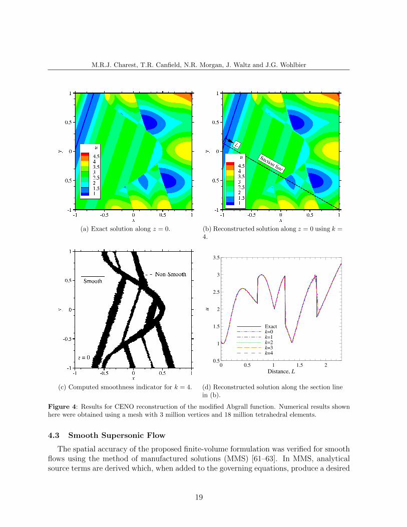
Eq. (50) was discretized on a cube with length 2 and centered about the origin, usingcomputational meshes similar to those used for the spherical cosine function (Fig. 3b). Areconstructed solution that was obtained with k = 4 is compared with the exact solutionalong z = 0 in Figs. 4a and 4b. This reconstruction was preformed on a mesh withapproximately 3 million vertices and 18 million tetrahedral elements, and, as observedin Fig. 4b, it was able to accurately represent the Abgrall function without producingspurious oscillations. This is because the smoothness indicator, illustrated in Fig. 4c,correctly identified the discontinuities in both u and ∂u/∂xi.

The solution obtained with k = 0 to 4 on a mesh with 18 million tetrahedral elements iscompared with the original function along a line in Fig. 4d. The proposed CENO schemewas able to ensure oscillation-free solutions despite the large discontinuities observed.This confirms the effectiveness of the smoothness indicator.

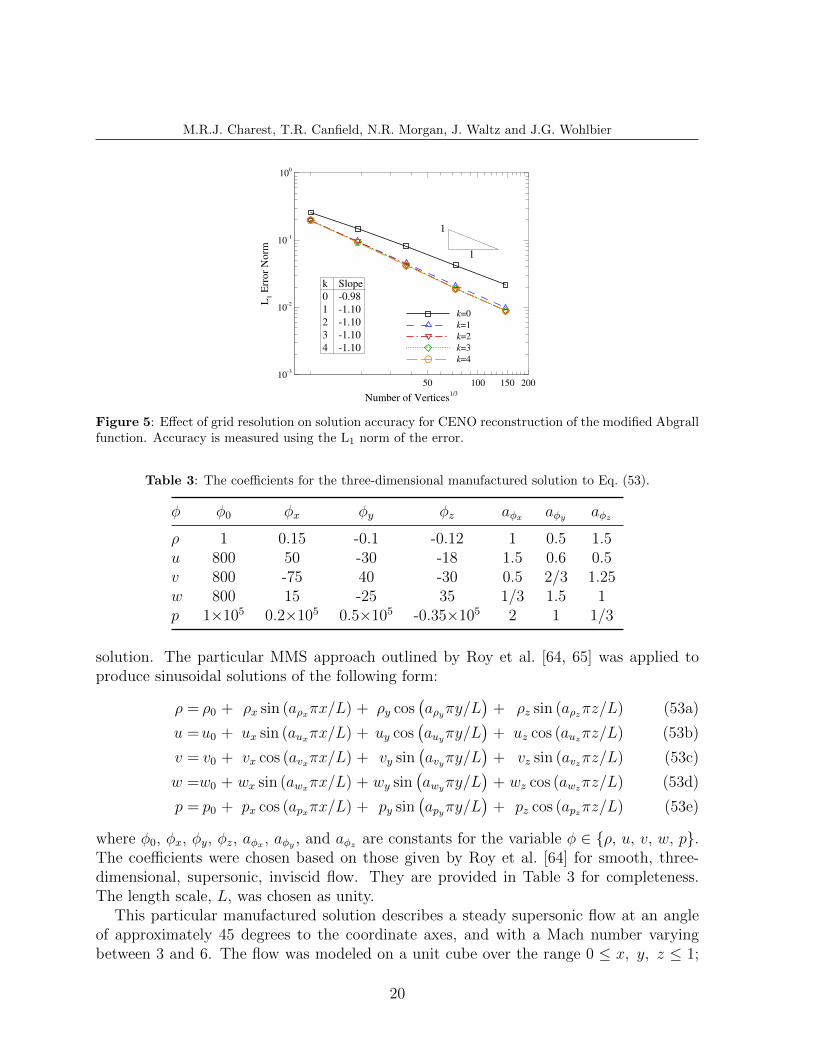
The effect of mesh resolution on the L1 norm of the solution error is illustrated inFig. 5. A large improvement in the error was achieved by increasing k from 0 to 1.This improvement became less pronounced as k was increased further to 2 since a largeportion of the domain possessed discontinuous features. In fact, because of the largenumber of discontinuities, there was only a slight improvement in the solution error as kwas increased beyond 2. This indicates that the solution error has not yet reached theasymptotic regime for this case.

The convergence rate of the error norms is also provided in Fig. 5. An order of accuracyof 1 was observed for all values of k, which was expected after applying a limited piecewiselinear reconstruction near discontinuous. Nonetheless, the main highlight is that thehybrid reconstruction procedure was able to produce non-oscillatory solutions despite thepresence of discontinuities, using only a single, central stencil.

18


(a) Exact solution along z = 0. (b) Reconstructed solution along z = 0 using k =4.

(c) Computed smoothness indicator for k = 4.

Distance, L

u

0 0.5 1 1.5 20.5

1

1.5

2

2.5

3

3.5

Exactk=0k=1k=2k=3k=4

(d) Reconstructed solution along the section linein (b).

Figure 4: Results for CENO reconstruction of the modified Abgrall function. Numerical results shownhere were obtained using a mesh with 3 million vertices and 18 million tetrahedral elements.

4.3 Smooth Supersonic Flow

The spatial accuracy of the proposed finite-volume formulation was verified for smoothflows using the method of manufactured solutions (MMS) [61–63]. In MMS, analyticalsource terms are derived which, when added to the governing equations, produce a desired

19



L1 E

rror

Norm

50 100 150 20010

3

102

101

100

k=0

k=1

k=2

k=3

k=4

1

1

k Slope

0 0.98

1 1.10

2 1.10

3 1.10

4 1.10

Figure 5: Effect of grid resolution on solution accuracy for CENO reconstruction of the modified Abgrallfunction. Accuracy is measured using the L1 norm of the error.

Table 3: The coefficients for the three-dimensional manufactured solution to Eq. (53).

φ φ0 φx φy φz aφx aφy aφz

ρ 1 0.15 -0.1 -0.12 1 0.5 1.5u 800 50 -30 -18 1.5 0.6 0.5v 800 -75 40 -30 0.5 2/3 1.25w 800 15 -25 35 1/3 1.5 1p 1×105 0.2×105 0.5×105 -0.35×105 2 1 1/3

solution. The particular MMS approach outlined by Roy et al. [64, 65] was applied toproduce sinusoidal solutions of the following form:

ρ = ρ0 + ρx sin (aρxπx/L) + ρy cos(aρyπy/L

)+ ρz sin (aρzπz/L) (53a)

u =u0 + ux sin (auxπx/L) + uy cos(auyπy/L

)+ uz cos (auzπz/L) (53b)

v = v0 + vx cos (avxπx/L) + vy sin(avyπy/L

)+ vz sin (avzπz/L) (53c)

w =w0 + wx sin (awxπx/L) + wy sin(awyπy/L

)+ wz cos (awzπz/L) (53d)

p = p0 + px cos (apxπx/L) + py sin(apyπy/L

)+ pz cos (apzπz/L) (53e)

where φ0, φx, φy, φz, aφx , aφy , and aφz are constants for the variable φ ∈ ρ, u, v, w, p.The coefficients were chosen based on those given by Roy et al. [64] for smooth, three-dimensional, supersonic, inviscid flow. They are provided in Table 3 for completeness.The length scale, L, was chosen as unity.

This particular manufactured solution describes a steady supersonic flow at an angleof approximately 45 degrees to the coordinate axes, and with a Mach number varyingbetween 3 and 6. The flow was modeled on a unit cube over the range 0 ≤ x, y, z ≤ 1;

20


although, any domain could be used since the solutions exist for all x, y and z. Anexample of this smoothly varying solution is illustrated in Fig. 6a, which depicts theinternal energy distribution.

The spatial accuracy was assessed by performing calculations with different mesh sizesand measuring the changes in solution error. Solutions were obtained on meshes of vary-ing resolution, similar to those in Fig. 3b, with supersonic inflow and outflow boundaryconditions at the corresponding upstream and downstream boundaries of the domain. Allsolutions were relaxed to a steady-state using the two-stage optimally smoothing schemeof Van Leer et al. [58] with a CFL = 0.5 and the HLL numerical flux. Any numericalflux can be used for this error analysis, because, according to Eq. (12), the dissipationvanishes with O(hk+1) for smooth solutions.

For each calculation, the analytical solution at every vertex of the primal mesh wasprescribed and the governing equations were relaxed until all equation residuals were re-duced by four orders of magnitude. Tighter tolerances were also tested, but no significantgain in accuracy was observed using them.

The L2 norm of the error in the predicted internal energy, e, is illustrated in Fig. 6b.All of the primitive solution quantities displayed the same relationship between mesh sizeand total solution error, but e displayed the largest errors, and was therefore chosen forthis analysis. The slopes of the lines in Fig. 6b are provided in Fig. 6c, along with thoseobserved for the other norms, i.e., the L1 and L∞ norms. For all values of interest fork, the formal order of accuracy was achieved by the L2 norm. The other norms alsodisplayed similar convergence characteristics, although some degradation of the slopes ofthe L∞ norms were observed as the mesh spacing decreased. This is largely attributedto the finite precision of the adaptive cubature algorithm used to evaluate the numericalerrors.

The solution error is plotted as a function of the wall-clock time in Fig. 6d. The high-order schemes become more efficient in terms of accuracy vs computational cost as thetarget accuracy gets smaller. That is, there is a particular range of accuracy for which aparticular value of k is the most efficient, and this optimal value of k increases with thedesired level of accuracy. For all the meshes considered, the first-order (k = 0) schemewas the least efficient, while the second-order (k = 1) scheme was the most efficient fora target error above about 103. Just below this level of error, the fourth-order (k = 3)scheme was the most efficient. The fifth-order (k = 4) scheme was the most efficient forerrors below 10. For this particular problem, there was no range over which the third-order (k = 2) scheme was optimal. These results confirm that, for smooth problems,higher-order schemes are more efficient for higher levels of desired accuracy.

4.4 Shock Tube

The robustness and accuracy of the algorithm was demonstrated for non-smooth prob-lems with a one-dimensional shock-tube [66]. This time-dependent problem was solved

21


(a) Exact solution.


L2 N

orm

of

Err

or

in e

20 40 60 80 10010

3

102

101

100

101

102

103

104

105

k=0

k=2

k=1

k=3

k=4

(b) Error in predicted e.

k Formal L1 L2 L∞

0 1 0.97 0.97 0.831 2 2.05 2.06 1.882 3 3.10 3.09 2.723 4 3.93 3.89 3.394 5 5.09 5.08 4.35

(c) Convergence of error norms.

WallClock Time (s)

L2 N

orm

of

Err

or

in e

100

101

102

103

104

103

102

101

100

101

102

103

104

105

k=0

k=2

k=1

k=3

k=4

(d) Solution time for a given accuracy.

Figure 6: Results for smooth supersonic flow.

on a rectangular domain of length 1, with the following initial conditions:

W(x, 0) =

WL if x ≤ 0.45,

WR if x > 0.45(54)

where WL = [1, 0, 0, 0, 1] and WR = [0.1, 0, 0, 0, 0.125]. A sample of the meshes usedis illustrated in Fig. 7 along with the dimensions of the computational domain.

Solutions were obtained for different values of k, using meshes of increasing resolution.All solutions were integrated in time until t = 0.2 s with the RK4 time-marching scheme,a CFL of 0.2, and the HLL numerical flux. Reflection boundary conditions were appliedto the surrounding surfaces while the solution was free to vary at both ends of the tube.

22


x

0.05L

L=1

Figure 7: Sample computational mesh and domain used for shock tube problem.

Solutions on the finest mesh considered are compared with the exact solution at t =0.2 s in Fig. 8a. Overall, there was a distinct improvement in the numerical solution asthe polynomial degree was increased, even near discontinuities. This is highlighted forthe contact surface in the inset of Fig. 8a. There was an initial large improvement inthe solution as k was increased from 0 to 1. Further increases in k provided smaller andsmaller improvements in the solution.

A similar comparison is made in Fig. 8b, which illustrates the effect of mesh resolutionon the fifth-order (k = 4) scheme. As expected, increasing the mesh resolution improvesthe agreement of the numerical solution with the exact solution. This occurs becausethere is less dissipation introduced by the time marching scheme, i.e., smaller time steps,and the spatial discretization, i.e., smaller grid spacing.

The behavior of the L1 error norms with mesh size is demonstrated for ρ in Fig. 8c. Thefirst-order (k = 0) scheme does not quite reach the asymptotic region. It only achievesan order of accuracy of approximately 0.7. The k = 1 scheme achieved a significantreduction in error over the k = 0 scheme, but only converges at a rate of O(h) due to thediscontinuities present in the solution. Using the coarsest mesh, all higher-order (k > 1)schemes had the same error as the linear representation. This is because the smoothnessindicator detected under-resolved data throughout most of the domain and the linearreconstruction was used everywhere. However, as the mesh resolution was increased, thehigher-order schemes had lower errors. All higher-order schemes only achieved first-orderaccuracy, which was expected because of the discontinuities in the solution, but there wasstill a decrease in overall error as k was increased beyond 1. Even though CENO dropsto first-order near discontinuities, the size of the region influenced by the discontinuitydecreases with mesh size. As such, there is a net reduction in error.

The computational efficiency was assessed in terms of the wall-clock time to a givenlevel of error. Over the range of meshes studied, the k = 1 scheme was the most efficient.However, extrapolating to lower error levels, the k = 2 scheme is expected to be moreefficient for error levels below 0.02. The efficiency of the other high-order schemes, i.e.,k = 3 and k = 4, is expected to improve as the desired error is lowered further.

23


x (m)

Den

sity

(kg/m

3)

0 0.2 0.4 0.6 0.8 10

0.2

0.4

0.6

0.8

1

1.2


(a) Effect of polynomial degree on predictions us-ing a mesh with 520,821 vertices.

x (m)D

ensi

ty (

kg/m

3)

0 0.2 0.4 0.6 0.8 10

0.2

0.4

0.6

0.8

1

1.2

Exact1,484 vertices9,654 vertices69,035 vertices520,821 vertices

(b) Effect of mesh size on predictions for k = 4.

k Slope

0 0.67

1 0.93

2 1.03

3 1.07

4 1.03


L1 N

orm

of

Err

or

in

20 40 60 80 10010

3

102

101

k=0

k=1

k=2

k=3

k=4

(c) Convergence of the error norms.

WallClock Time (s)

L1 N

orm

of

Err

or

in

100

101

102

103

104

105

106

107

103

102

k=0

k=1

k=2

k=3

k=4

(d) Accuracy as a function of solution time.Dashed lines represent extrapolations.

Figure 8: Results for one-dimensional shock-tube at t=2 s.

4.5 Sedov Blast Wave

The Sedov explosion problem [67] involves the evolution of a spherical blast wave froman initial pressure perturbation in an otherwise homogeneous medium. The blast wavewas generated by an initial energy source, eblast, located in a small region of radius r0 near

24


Figure 9: Sample computational mesh used for Sedov problem.

the origin. The initial conditions at time t = 0 are

ρ(r, 0) = 1, ~v(r, 0) = ~0, p(r, 0) =

3 ρ (γ − 1) eblast

4πr30

if r ≤ r0

10−5 if r > r0

where r =√x2 + y2 + z2, eblast = 0.851072. This configuration gives a blast wave that

reaches r = 1 at t = 1 s.In practice, it is difficult to define a small radius r0 without an overly fine mesh near the

origin, especially when using tetrahedral mesh. So the energy eblast was deposited into thecontrol volume at the origin only. Simulations were obtained with k = 0, 1, . . . , 4 on fourdifferent, successively-refined meshes. All solutions were integrated in time until t = 1 swith the RK4 time-marching scheme, a CFL of 0.1, and the Rusanov numerical flux.Only an octant of a sphere was modeled, with reflecting boundary conditions to enforcesymmetry. The outer surface of the sphere, located at R = 1.2 m, was also treated as areflecting wall. A sample computational mesh is illustrated in Fig. 9.

Predictions for density are compared with the analytical solution in Fig. 10. The exactsolution for this spherical blast wave was obtained using the numerical algorithm outlinedby Kamm [68]. For all values of k and meshes employed, no oscillations were observed infront of or behind the diverging shock wave. For the high-order solutions, i.e., k > 1, thesmoothness indicator correctly identified the large solution discontinuity at the movingshock front

The effect of polynomial order on the predicted density is illustrated in Fig. 10a for thefinest mesh investigated (844,701 vertices and 4,922,880 tetrahedra). As also observedfor the shock tube test problem in Section 4.4, increasing the order of the polynomialprovided a significant improvement in the predicted solution.

Figure 10b illustrates the effect of mesh resolution on the predicted density, which

25


x (m)

Den

sity

(kg/m

3)

0 0.2 0.4 0.6 0.8 1 1.20

1

2

3

4

5

6


(a) Effect of polynomial degree on predictions us-ing a mesh with 844,701 vertices.

x (m)D

ensi

ty (

kg/m

3)

0 0.2 0.4 0.6 0.8 1 1.20

1

2

3

4

5

6

Exact1,999 vertices14,364 vertices108,655 vertices844,701 vertices

(b) Effect of mesh size on predictions for k = 4.

Figure 10: Results for the Sedov problem at t = 1 s.

was obtained using the 5th-order (k = 4) CENO reconstruction. At low resolutions, thesmoothness indicator flagged a large portion of the domain as under-resolved. However,as the mesh resolution was increased, the size of the region treated using the lower-orderlimited piecewise linear reconstruction diminished.

4.6 Triple-Point Shock Interaction

As a final test of the algorithm’s robustness, a three-dimensional, three-state Riemannproblem was studied. The initial conditions, which are illustrated in Fig. 11 along withthe geometry, generate a shock that propagates parallel to a contact discontinuity, whichin turn generates a high-speed vortex. This problem does not have an exact solution,but it is studied here because of the difficulty in resolving the interaction between theshocks and contact discontinuities without generating spurious oscillations, especially forhigh-order solution methods.

Two simulations were obtained on mesh with approximately 347,811 vertices and1,960,914 tetrahedra, one with a low-order representation (k = 1) and one with a high-order (k = 4) polynomial representation. Both solutions were integrated in time untilt = 5 s with the RK4 time-marching scheme, a CFL of 0.25, and the HLL numerical flux.Reflection and solid wall boundary conditions were applied as indicated in Fig. 11.

Numerical predictions for density at t = 5 s are compared in Fig. 12. No significantdifferences between the two solutions were visible, because the high-order CENO schemedeemed a large portion of the flow non-smooth and it was treated using the limited linearreconstruction instead. These results highlight the robustness of the high-order CENOalgorithm, since the k = 4 scheme was able to reliably obtain a solution without producing

26


ρ = 0.1p = 0.1

ρ = 1.0p = 0.1

p = 1.0ρ = 1.0

17

1

3

Solid Walls

Reflection

Figure 11: Computational domain and initial conditions for the triple-point problem.

Figure 12: Predicted density field at t = 5 s for triple-point problem.

any unphysical oscillations.

5 CONCLUSIONS

A high-order finite-volume scheme was developed for the mathematical description ofcompressible fluids on unstructured meshes. It is a vertex-based variant of the cell-based,

27


Godunov-type, finite-volume methods developed by Ivan et al. [36–40] and Charest et al.[32–35], which use a hybrid CENO reconstruction procedure to avoid spurious oscillations.The scheme was assessed in terms of accuracy and computational cost for a variety ofproblems, including smooth and discontinuous function reconstructions, and solutions toidealized flow problems.

Up to fifth-order accuracy was demonstrated. For smooth flows and function recon-structions, (k + 1)th order of accuracy was achieved using piecewise polynomial repre-sentations of degree k. Only first-order accuracy was observed for all problems thatcontained discontinuities, but there was still a measured advantage provided by the high-order schemes. They displayed lower errors for a given mesh.

In terms of computational efficiency, i.e., wall time for a given accuracy, there wasan optimal value of k which varied depending upon the desired error, and the particularproblem. The standard second-order scheme was the most efficient for higher error levels,and the high-order schemes became more efficient as the desired error was decreased.This was demonstrated for smooth and discontinuous problems, although the mesh sizes atwhich the high-order schemes were more efficient was significantly larger for discontinuousproblems.

Overall, this research highlights the main advantages of the CENO finite-volume al-gorithm. High-order accuracy was achieved in smooth regions, while robust and mono-tone solutions were maintained near discontinuities and under-resolved solution content.Future work consists of further development and validation of the proposed algorithm,including its extension to multi-material problems, arbitrary equations of state, movingmeshes, and adaptive mesh refinement.

ACKNOWLEDGMENTS

This research was supported by the United States Department of Energy, throughthe Advanced Simulation & Computing (ASC) and Metropolis postdoctoral fellowshipprograms.

REFERENCES

[1] D.J. Mavriplis. AIAA J., 46(6):1281–1298, 2008.

[2] S. Pirozzoli. J. Comput. Phys., 219(2):489–497, 2006.

[3] A. Harten, B. Engquist, S. Osher, and S.R. Chakravarthy. J. Comput. Phys., 71(2):231–303, 1987.

[4] T.J. Barth. AIAA Paper 93-0668, 1993.

[5] R. Abgrall. J. Comput. Phys., 114:45–58, 1994.

[6] T. Sonar. Comp. Meth. Appl. Mech. Eng., pp. 140–157, 1997.

28


[7] C.F. Ollivier-Gooch. J. Comput. Phys., 133:6–17, 1997.

[8] G.S. Jiang and C.W. Shu. J. Comput. Phys., 126(1):202–228, 1996.

[9] D. Stanescu and W. Habashi. AIAA J., 36:1413–1416, 1998.

[10] O. Friedrich. J. Comput. Phys., 144(1):194–212, 1998.

[11] C. Hu and C.W. Shu. J. Comput. Phys., 150:97–127, 1999.

[12] C.F. Ollivier-Gooch and M. Van Altena. J. Comput. Phys., 181(2):729–752, 2002.

[13] A. Nejat and C. Ollivier-Gooch. J. Comput. Phys., 227(4):2582–2609, 2008.

[14] B. Cockburn and C.W. Shu. Math. Comp., 52:411, 1989.

[15] B. Cockburn, S. Hou, and C.W. Shu. J. Comput. Phys., 54:545, 1990.

[16] R. Hartmann and P. Houston. J. Comput. Phys., 183:508–532, 2002.

[17] H. Luo, J.D. Baum, and R. Lohner. J. Comput. Phys., 225:686–713, 2007.

[18] G. Gassner, F. Lorcher, and C.D. Munz. J. Comput. Phys., 224(2):1049–1063, 2007.

[19] F. Bassi and S. Rebay. J. Comput. Phys., 131:267–279, 1997.

[20] B. Cockburn and C.W. Shu. SIAM J. Numer. Anal., 35(6):2440–2463, 1998.

[21] B. Leervan , M. Lo, and M. Raaltevan . AIAA Paper 2007-4083, 2007.

[22] M. Raaltevan and B. Leervan . Commun. Comput. Phys., 5(2–4):683–693, 2009.

[23] H. Liu and J. Yan. SIAM J. Numer. Anal., 41(1):675–698, 2009.

[24] Z.J. Wang. J. Comput. Phys., 178:210–251, 2002.

[25] Z.J. Wang and Y. Liu. J. Comput. Phys., 179:665–697, 2002.

[26] Z.J. Wang, L. Zhang, and Y. Liu. High-order spectral volume method for 2d eulerequations. Paper 2003–3534, AIAA, June 2003.

[27] Z.J. Wang and Y. Liu. Journal of Scientific Computing, 20(1):137–157, 2004.

[28] Y. Sun, Z.J. Wang, and Y. Liu. J. Comput. Phys., 215(1):41–58, 2006.

[29] H. Huynh. AIAA Paper 2007-4079, 2007.

[30] Z.J. Wang and H. Gao. AIAA Paper 2009–401, 2009.

29


[31] Z.J. Wang and H. Gao. J. Comput. Phys., 228:8161–8186, 2009.

[32] S.D. McDonald, M.R.J. Charest, and C.P.T. Groth. High-order CENO finite-volumeschemes for multi-block unstructured mesh. 20th AIAA Computational Fluid Dy-namics Conference, Honolulu, Hawaii, June 27–30 2011. doi: 10.2514/6.2011-3854.AIAA-2011-3854.

[33] M.R.J. Charest, C.P.T. Groth, and P.Q. Gauthier. High-order CENO finite-volumescheme for low-speed viscous flows on three-dimensional unstructured mesh. ICCFD7- International Conference on Computational Fluid Dynamics, Hawaii, July 9–132012. Paper ICCFD7-1002.

[34] M.R.J. Charest and C.P.T. Groth. A high-order central ENO finite-volume schemefor three-dimensional turbulent reactive flows on unstructured mesh. 21st AIAAComputational Fluid Dynamics Conference, San Diego, California, June 24–27 2013.doi: 10.2514/6.2013-2567. AIAA 2013-2567.

[35] M.R.J. Charest, C.P.T. Groth, and P.Q. Gauthier. Commun. Comput. Phys., 2013.Submitted for publication.

[36] L. Ivan and C.P.T. Groth. AIAA paper 2007-4323, 2007.

[37] L. Ivan and C.P.T. Groth. AIAA paper 2011-0367, 2011.

[38] L. Ivan and C.P.T. Groth. Commun. Comput. Phys., 2013. submitted for publication.

[39] L. Ivan and C.P.T. Groth. J. Comput. Phys., 257:830–862, 2013.

[40] A. Susanto, L. Ivan, H. De Sterck, and C.P.T. Groth. J. Comput. Phys., 250(1):141– 164, 2013.

[41] A. Haselbacher. AIAA paper 2005-0879, 2005.

[42] J. Waltz, N.R. Morgan, T.R. Canfield, M.R.J. Charest, L.D. Risinger, and J.G.Wohlbier. Comput. Fluids, 92:172–187, 2013.

[43] C.A. Felippa. Eng. Computation., 21(8):867–890, 2004.

[44] T.J. Barth and P.O. Fredrickson. AIAA Paper 90-0013, 1990.

[45] D.J. Mavriplis. AIAA paper 2003-3986, 2003.

[46] A. Jalali and C. Ollivier-Gooch. AIAA Paper 2013-2565, 2013.

[47] C.L. Lawson and R.J. Hanson. Solving least squares problems. Prentice-Hall, 1974.

[48] K. Michalak and C. Ollivier-Gooch. AIAA paper 2007-3943, 2007.

30


[49] N.R. Draper and H. Smith. Applied regression analysis. Wiley, New York, 3rdedition, 1998.

[50] T.J. Barth. AIAA Paper 91-1548, 1991.

[51] J.S. Park, S.H. Yoon, and C. Kim. J. Comput. Phys., 229(3):788–812, 2010.

[52] V. Venkatakrishnan. AIAA Paper 93-0880, 1993.

[53] S.K. Godunov. Mat. Sb., 47:271–306, 1959.

[54] V.V. Rusanov. J. Comput. Math. Phys. USSR, 1:267–279, 1961.

[55] S.F. Davis. SIAM J. Sci. Stat. Comput., 9(3):445–473, 1988.

[56] A. Harten, P.D. Lax, and B. Leervan . SIAM Rev., 25(1):35–61, 1983.

[57] H. Lomax, T.H. Pulliam, and D.W. Zingg. Fundamentals of Computational FluidDynamics. Springer, New York, 2003.

[58] B. Van Leer, C. Tai, and K.G. Powell. AIAA Paper 89-1933, 1989.

[59] J. Berntsen, R. Cools, and T.O. Espelid. ACM Trans. Math. Softw., 19(3):320–332,1993.

[60] R. Abgrall. ICASE Contractor Report 189574, 1991.

[61] P.J. Roache and S. Steinberg. AIAA J., 22(10):1390–1394, 1984.

[62] W.L. Oberkampf and F.G. Blottner. AIAA J., 36(5):687–695, 1998.

[63] P.J. Roache. J. Fluids Eng., 124(1):4–10, 2001.

[64] C.J. Roy, T.M. Smith, and C.C. Ober. AIAA Paper 2002-3110, 2002.

[65] C.J. Roy, C.C. Nelson, T.M. Smith, and C.C. Ober. Int. J. Numer. Meth. Fluids, 44(6):599–620, 2004.

[66] G.A. Sod. J. Comput. Phys., 27(1):1 – 31, 1978.

[67] L.I. Sedov. Similarity and Dimensional Methods in Mechanics. Academic Press, NewYork, 1959.

[68] J. Kamm. Evaluation of the Sedov-von Neumann-Taylor blast wave solution. Tech-nical Report LA-UR-00-6055, Los Alamos National Laboratory, 2000.

31

A VERTEX-BASED HIGH-ORDER FINITE-VOLUME...

Documents

Transcript of A VERTEX-BASED HIGH-ORDER FINITE-VOLUME...