A VARIATIONAL METHOD FOR MULTISTAGE LAUNCH

VEHICLE OP TIMIZATION

by Fred Teren and Omer F. Spurlock

Lewis Research Center

Cleveland, Ohio

TECHNICAL PAPER proposed for presentation at

Third Aerospace Sciences Meeting of the American

Institute of Aeronautics and Astronautics

New York, New York, January 24-26, 1966

NATIONAL AERONAUTICS AND SPACE ADMINISTRATION

https://ntrs.nasa.gov/search.jsp?R=19660005481 2020-03-06T07:45:28+00:00Z

A -¢A_R!ATIONAL METHOD .VOR ,MULTISTAGE LAUNCH -VEHICLE OPTIMIZATION

by Pred Teren and Omer F. Spurlock

Lewis Research Cer_ter

National Aeronautics and Space Ad_ministration

Cleveland, Ohio

/)

ABSTRAC [ O

The methods of the calculus of variations are used to maxLmize payload

capability for multistage launch vehicles. The method of solution uses the

Lagrange r.m_=p__ez s to dete=_r_ine the opt_mm'a thrust direction profile, as

_ell as to construct partial derivatives of payload with respect to the stage

_:ropellant loadings and a booster steering parameter. These derivatives are

u,sed to _e_,_.±__ate__'_ " the stages and/or as te_ainal equations to be satisfied

!,&_x_zum payloaff can thus be achieved with a single solution, rather than with

a f_iiy of parametric results. Constant t_must and specific-£._pulse opera-

tion is ass-mued for each upper stage (booster thrust and specific ]_mpulse

vary with atmospheric pressure), and structure weight can be either fixed or

a linear function of the stage propellant loading. Two-dimensional flight

in a central, inverse-s_uare gravitational field is ass_med.

N'_.eriaa! results are presented for two- and three-stage launch vehicles

flown to cir:_'u!ar orbit and Earth escape, respectively. Parametric results

are presented a:td compared with the overall optlm"_,_ solution obtained by use

o,, &jj,j_,_e variationa" technique.

INTRODUCTION

A problem that frequently arises in trajectory optimization studies is

that of determining the maximum payload capability of a multistage launch

vehicle f!ovn to a prescribed set of burnout conditions. If all vehicle pa-

r_aeters are specified, the problem reduces to that of finding the opt£mum

X-53150

steering profile. In many cases, however, not all these parameters are speci-

fied 3 and those left unspecified can be varied to maximize payload.

A typical situation that occurs in the design of future launch vehicles

is one in which the stage thrust levels and propellant flow rates (and, for

practicality, the gross launch weight) are specified, but some or all the

stage propellant loadings are left unspecified. The unspecified propellant

loadings generally can be varied to achieve maximum payload capability for

the vehicle.

An additional optimizing parameter frequently is available in the booster

steering program. Since the booster stage operates in the atmosphere, the

booster thrust direction profile is shaped to minimize aerodynamic heating

and loads and is not available for complete optimization. A single degree

of freedom remains, however, corresponding to the magnitude of a short pitch-

over phase following the initial vertical rise. This degree of freedom, some-

times called the booster kick angle, determines the amount of trajectory loft-

ing during boost phase. Since the upper stages operate essentially under

vacuum conditions, the steering program for these stages is available for

complete optimization.

Many authors (e.g., refs. 1 to 7) have treated the problem of optimizing

the stage propellant loadings of multistage vehicles. None of these authors,

however, has attempted to optimize the steering program for these vehicles.

Others (e.g., refso 8 to lO) have used the calculus of variations to optimize

the steering program for various rocket vehicles. In particular, reference ll

treats the problem of optimizing the steering program of a multistage launch

vehicle. Reference ll, however, does not consider the problem of optimizing

the stage propellant loadings or booster kick angle.

Recently, Mason, Dickerson, and Smith (ref. lg) have considered the prob-

lem of simultaneously optimizing the steering program and the stage propellant

2

loadings of a multistage launch vehicle. These authors followed the approach

of Denbow(ref. 13) and Hunt and Andrus (ref. 14) in formulating the variational

problem.

The present report waswritten concurrently with reference 12 and presents

a method which allows the propellant loadings, booster kick angle, and upper-

stage steering program to be simultaneously optimized. The variational approach

is somewhatdifferent from that used in reference 12. By following the method

of reference iS, the maximizing functional is written as the sumof the final

payload and a constraint integral for each of the upper stages. The resulting

boundary equations supply partial derivatives of payload with respect to the

unspecified parameters. These derivatives are then used, along with the re-

quired burnout conditions, as terminal equations to be satisfied. The analysis

does not require that all the stage propellant loadings (or booster kick angle)

be optimized. Equations are developed for optimizing payload with respect to

any combination of unspecified parameters.

The variational equations for optimizing vehicle pars_metershave been in-

corporated into a digital computer program used previously at Lewis for para-

metric Launch-vehicle studies. Someof the procedures used to obtain numeri-

c_alresults with this program are discussed in reference 16. Numerical results

are p__ese_tedfor two- and three-stage launch vehicles flown to circular orbit

a._dia_'th escape, respectively, to demonstrate the feasibility of the varia-

tional approach. Parametric results are presented showing the variation of

payload with propellant loadings and booster kick angle. The resulting pay-

load envelopes are then comparedwith the overall optimum points generated

directly by meansof the variational technique in order to verify the equations.

ANALYSIS

The _roblem to be solved is to determine the maximumpayload capability

of an N-stage launch vehicle flown to a specified set of burnout conditions.

3

The analysis admits atmospheric effects during booster phase but assumesvacuum

operation for all other stages. Becauseof these atmospheric effects, the

booster steering program is assumedcompletely specified (e.g., zero angle of

attack), except for the booster kick angle. The upper-stage steering program,

however, is unconstrained and is determined to maximize payload. The calculus

of variations is used for this purpose.

Each of the upper stages is assumedto operate at a fixed (constant) value

of thrust and propellant flow rate. These values maybe zero_ so that coast

phases are admitted. The structure massfor each stage is assumedto be a

linear function of the stage propellamt loading, defined by

ms = mH + kmp

where ms is the total structure mass, mH is the fixed mass, mp is the stage

propellant mass, and k is the propellant sensitive mass fraction. (All sym-

bols are defined in appendix A.)

In addition to the variational trajectory, provision is also madefor add-

ing an additional velocity increment &vi after the desired orbit conditions

are achieved. This velocity increment is achieved by use of the final stage

for propulsion. The amount of propellant required for this maneuver is calcu-

lated by use of the standard impulsive velocity equations.

Variational Problem

Since the booster steering program is not subject to complete optimization,

the booster stage is not treated in the following EuleroLagrange equations.

The booster degrees of freedom (propellant loading and kick angle) are included

by allowing variations in the position and velocity at second-stage ignition.

The associated equations, along with the equations for optimizing upper-stage

propellant loadings, are treated in the boundary equations resulting from the

variational analysis.

The variational problem to be solved is that of finding the upper-stage

4

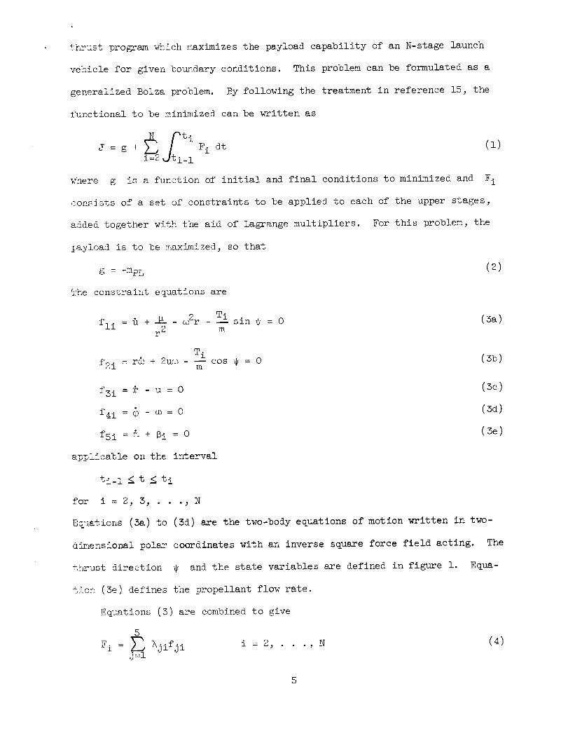
thrust pro_am which m_ximizes the payload capability of an N-stage launch

vehicle for given boundary conditions. This problem can be formulated as a

generalized Bolza problem. By following the treatment in reference 15, the

functional to be minimized can be written as

i_2_t.1 tiJ = g + Fi dt (i)°= --1

where g is a function of initial and final conditions to minimized and Fi

consists of a set of constraints to be applied to each of the upper stages,

added together with the aid of Lagrange multipliers. For this problem, the

_yload is to be maximized, so that

g = _mp L (2 )

_'he constraint equations are

fli = _ + _L _ _lr - --Tisin _ = 0 (3a)r 2 m

T ifli = r& + 2u_ - -- cos @ = 0 (3b)m

f3i = _ - u = o (5c)

f_i : _ - _ : o (3d)

fsi = i + _i = 0 (3e)

applicable on the interval

ti_ I _ t _ ti

for i = 2, 3, . ._ N

Ec_.ations (3a) to (Zd) are the two-body equations of motion written in two-

di_ensional polar coordinates with an inverse square force field acting. The

t_ust direction W and the state va_iables are defined in figure i. Equa-

t[on (3e) defines the propellant flow rate.

Equations (S) are combined to give

5

F i = _ hjifji i = 2,

j=l

., N (4)

where 7`ji are undetermined Lagrange multipliers, which are functions of time

since the constraint equations must be satisfied at all points of the trajectory.

Euler-Lagrange Equations

As shown in reference 17, a necessary condition for g to be minimized

is that the Euler-Lagrange equations be satisfied. The Euler-Lagrange equa-

tions are

i = 2, ., N; j = i, ., 6 (5)

where xj are the problem variables

Xl(t)= u_

x2(t) = _o

x3(t) = r

x4(t)=

xs(t) = m

x6(t)= _.

(6)

The Euler-Lagrange equations for the present problem can be written explicitly

by use of equations (3) and (A):

i

hl = 2mh2 - 7`3 (7a)

u 7`4

7`2= -z_°7`l+ 7 7`2- T (7b)

_3 = -C_ + °D2)7`1 +_2S (7c)

_4 : o (7d)

= T_5 m-_ (7`1 sin @ + 7`2 cos _/) (7e)

(7`1cos _ - 7,2 sin _)_ = o (7f)

Equations (7) (and subsequent equations) apply separately to each of the upper

stages. The subscript i has been omitted for simplicity.

Equation (7f) determines the thrust direction (for T _ 0):

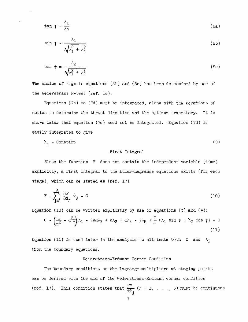
h1tan _ = ?`-_ (Sa)

?`lsin _ = (Sb)

2

?'2(sc)COS _/ =

The choice of sign in equations (8b) and (8c) has been determined by use of

the Weierstrass E-test (ref. 18).

Equations (7a) to (7d) must be integrated_ along with the equations of

motion to determine the thrust direction and the optimum trajectory. It is

shown later that equation (7e) need not be integrated. Equation (7d) is

easily integrated to give

h 4 = Constant (9)

First Integral

F does not contain the independent variable (time)Since the function

explicitly 3 a first integral to the Euler-Lagrange equations exists (for each

stage), which can be stated as (ref. 17)

F - _ xj = C (lO)

Equation (i0) can be written explicitly by use of equations (3) and (4):

(r-_2 r) + T (?`i sin ? + ?`2 cos ?) = 0_ . 2 hi - 2u_h2 + uh5 _h4 - _?`5 +mC

(ll)

Equation (ii) is used later in the analysis to eliminate both C and h5

from the boundary equations.

Weierstrass-Erdmann Corner Condition

The boundary conditions on the Lagrange multipliers at staging points

can be derived with the aid of the Weierstrass-Erdmann corner condition

8F(ref. 17). This condition states that _ (j = i, ._ 6) must be continuous

7

at such corners. For the present problem, this condition implies that all the

multipliers are continuous at staging points, hence continuous throughout the

traj ect ory.

Transversality Equation

The relation betweenchanges in boundary conditions and changes in J is

expressed by the general transversality equation (ref. 17). For this problem,

the transversallty equation can be written

_[_I j___ _ j____il _F I ti

6 3" _ 6

dJ = - _j dt + x_j dx + dg (12)

Jti-i

This equation can be written explicitly by using the definition of F and the

first integral

N )t idJ = l_= (Cidt + %1 du + rh 2 d_ + h 3 dr + %4 d_ + h 5 dm i ti-1 + dg (13)

The subscript i has been used with C and dm since these variables may

be discontinuous at staging points.

Boundary Equations

If some of the problem variables (state conditions or control variables)

are not specified, values should be chosen which minimize J (or, equivalently,

maximize payload).

According to reference 17, minimizing J is accomplished by setting dJ

equal to zero. Equation (13) has the form

m

dJ = _ Gj dxj = 0 (14)

If the m problem variables xj are all independent, dJ wil vanish if, and

only if, each term on the right side of equation (14) is independently set equal

to zero. For specified variables xj, the allowable variation dxj is zero;

for unspecified xj, the coefficient Gj must be set equal to zero. Equa-

8

tion (la) can thus be interpreted as a total differential of J, and

8JGj =

J

Equation (13) is not suitable for this interpretation, since the variables are

not all independent. In the following section the dependent variables are

eliminated by expressing the dependence explicitly.

Consider first the terms in equation (13) involving the variations of the

state variables.

i du + rh 2 de + h3 dr + ha d_ ti_l (h I du) + - (hI du)- + (rh 2 de) +

de)- + (h 3 dr) + - (h3 dr)- + (h a d_) + (ha d_0)-]t=t i(rh2

+ (hI du + rh 2 de + h 3 dr + h a d_)t=t_ - (hI du + rh 2 de + h 3 dr + h a d_)t=t_

(is)

where the superscripts - and + refer to conditions before and after staging,

respectively. Since the state variables and Lagrange multipliers are continuous

throughout the trajectory, the summation on the right side of equation (15) is

identically zero. At t = tl, the variations in state conditions are due to

the allowable variations in booster burning time and kick angle.

j = i, ., a (16)

TI is the booster burning time.

is the burning time of stage i, that is, Ti = t i - ti_l).

8xj_xJ dT I d_

(dxj)t=t_ = ST1 + _

where _ is the booster kick angle and

general, Ti

generality, the state variations at

of generalized (independent) state variables, qk' k = i, .

_xjdxj = _ d_k j = i, o, a

k=l

Combining equations (15) to (17) yields

(In

For

t = tN are expressed in terms of a set

., a, so that

(17)

8u 8_ 8r(kI du+rh 2 d_+h 3 dr+h 4 d@)ti = 1 _+rh2 _+h3 _+h4

- 1 _+rh2 _+h3 _+h4 =t{d_- 1 m_1 T_1 +h3 T_1 +h4 t=t dT1

(18)

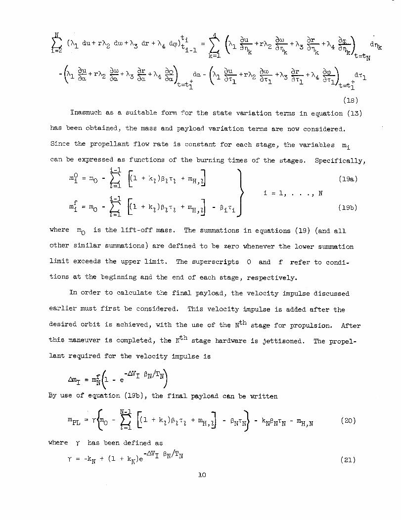
Inasmuch as a suitable form for the state variation terms in equation (IZ)

has been obtained; the mass and payload variation terms are now considered.

Since the propellant flow rate is constant for each stage; the variables m i

can be expressed as functions of the burning times of the stages. Specifically;

i-im0 =mo - _ [i + k_)_T_ +mH, (19a)

i =i; .; N

m'fl = mo - _ i + kZ)BZT z + _H, - _iTi (19b)

where m0 is the lift-off mass. The summations in equations (19) (and all

other similar summations) are defined to be zero whenever the lower summation

limit exceeds the upper limit. The superscripts 0 and f refer to condi-

tions at the beginning and the end of each stage; respectively.

In order to calculate the final payload; the velocity impulse discussed

earlier must first be considered. This velocity impulse is added after the

desired orbit is achieved_ with the use of the Nth stage for propulsion. After

this maneuver is completed_ the Nth stage hardware is jettisoned. The propel-

lant required for the velocity impulse is

Ami= mf(1 - e-AVI _N/TN)

By use of equation (19b), the final payload can be written

mpL = Y_O- _ [_(i + kZ)_ZTZ +mH, _ - _NTN) kN_NTN - mH, N (20)

where y has been defined as

y = -kN + (i + kN)e -AVI _N/TN (21)

i0

The variations din0' droll' and dmpL can nowbe expressed in terms of the

variations in burning times by differentiating equations (19) and (20).

0E (1 + kZ)BZ dTZdm i =-Z=I

f(i + kZ)_Z dT Z - _i dTidm i = _

Z=I

i =i_ ., N

(22a)

(z2b)

N-I

dmpL =-y_ (1 + kZ)BZ dTZ - (]_ + kN)SN d_ N(22c)

By use of equations (22), the terms in equation (15) involving dm i can be

simplified and expressed in 9ez_m{ of %he variations dT.i

• : P2 '_ki_idh - _ (i + ki)_i d_i(?\5 dmi) -i "= m:!

+ +kl) 1 1 (2s)

where

i

_5 --(_5)t t'-----i

Also, the time variation tem_zs in eiuation (15) can be expressed in terms of

variations in the stage burning tLmes:

= Ci dT i(Ci dr) -i(2_)

The variation of g is -alculated by combining equations (2) and (22c) :

dg = _ _ (l + ki)_i dTi + (_ + k_)_ a'_N(25)

The variable ZN can be eliminated from equation (25) by use of the following

identity :

It is convenient to define

ii

sf. ci • -, (27a)

s_ : o _i : o

0Si : 0 _i : 0

i=2, ., N

SI = - _q i T_ I + rh2 T_ I + hS T_ I + h4

Also, note that i5 = 0 i'or coast phases, so that for T i = O,

By use of equations (27) and (28), equation (26) becomes

Equations (16) to (18), (23) to (25) and (29) are now combined with equa-

tion (51) to give

N-I (([y_. ki)_idJ= m_.I 1 +

N

Z=

(ZTb)

(27c)

(27d)

(27e)

(28)

(29)

N

_i=O

Ci dTi + Y + kN)_N + _N dTN - _i _ + r_2 + hS _ + _ _ t=tl

+ = 1 _j+rh2 _+ hs_r-E-+h4_l d_j :0

_J _J d It=tN

(so)

The variations in equation ($0) are all independent, so that the form of equa-

tion (14) has been achieved, with

oIO(_i) : (1 + ki)_i + (S - S + _i i' _i _ 0Z=

i=l, •, N-I

(31a)

12

a(Ti) : ci, _i : 0 i = 2, . ., N - 1 (3lb)

o(T N) = (_ + k_)_ + _s_ (31c)

o(_) : - i + rhz + _3 _ + h4t=t I

(31d)

G(_j ) : 1

:tN

j = i, • • ., _ (31e)

Prom equations (ii) and (27),

-_?-r _]. + 2u_oh2 uls - _4 mf i

_f t=ti°i = (32_)

-a_2 hi + 2u<oh2 - uh3 - _°_'4: - m-'_-. + _

sO = l t=ti_ I (32b)

i=2, ., N;

h/o

(32c)

Since equations (52) do not contain C or _5' equation (7e) need not be inte-

grated to evaluate equations (31), as indicated earlier.

Boundary Value Problem

The determination of' an optimum trajectory requires the simultaneous

integration of the equations of motion and the Euler-Lagrange equations. A set

of initial conditions (state variables and La_ange multipliers) and staging

times is required in order to specify the trajectory uniquely.

The trajectory thus generated must satisfy N + 5 final conditions, corre-

sponding to the N + 5 independent problem variables in equation (30). For

specified variables, the final conditions have the form

xj : xj, d (33)

where the subscript d indicates the desired final value. For unspecified vari-

ables, equations (31) supply auxiliary final conditions with the form

i3

o(xj) = o

Some of equations (33) are easily satisfied; for example, a specified burn-

ing time for any stage can be achieved simply by terminating that stage at the

proper time during the integration. An iteration is required in order to satisfy

the nontrivial final conditions, and variable initial conditions (equal to the

number of final conditions) must be available. For the present problem, the

Lagrange multipliers (hi, i = i, ., 4), the burning times of all stages

being optimized, and the booster kick angle (if it is being optimized) are avail-

able as variable initial conditions.

The size of the iteration loop can be reduced by using the fact that equa-

tions (7) are homogeneous in the h's. This implies that the choice of any one

is arbitrary and serves only as a scale factor for the others. The value of

this multiplier can be chosen to satisfy one of equations (31).

The iteration size can be further reduced when Z4 = 0 is a required final

condition, which occurs when the travel angle is unspecified (ref. 8). Since hA

is a constant and is continuous across staging, this final condition can be satis-

fied at t = tl; h 4 is thus removed from the iteration. Equation (31d) can also

be evaluated at t = tl, and the booster kick angle optimization can be similarly

removed from the iteration.

The burning times of optimized stages can sometimes be removed from the

iteration, along with an equal number of equations (31). The principle involved

is similar to that used in removing equation (_ld): If all variables in the

equation G(T_) = 0 can be calculated at (or previous to) t = t_, stage _ can

be terminated (during stage _) whenever the optimizing equation is satisfied.

The number of optimized stages which can be thus removed depends on the charac-

teristics of the particular problem.

Consider first two powered stages TZ and Tm, _ < m, with km _ O. Equa-

tion (31a) must be set equal to zero for i = Z and i = m, and the two result-

_ug equations are combined to give

m-i

2 "+ -s0l÷1+l+k Z

i=Z+l

(35)

E_ation (3!a) (for i = Z) can be satisfied by the choice of one of the _'s.

Equation (35) contains terms which can all be calculated at, or prior to, stage

m cutoff, and this equation can be used to terminate stage m. Specifically,

s+9,ge m is terminated when

s : _-_-= ' - (sf- s (3s)m m k_o" i + k t l

i=Z +I

If _ : O, the term in Sm disappears from equation (35), and this equation can

then be used to terminate stage m - i:

m-i m-2

-i m = i - Si

i=Z +i i:Z +il+kz

m > Z + i (37a)

_f

SO- °Z - 0 m = Z + i (37b)m i +k Z

The terms on the left side of equations (37) are evaluated at stage m - i cut-

off, and the terms on the right side are eval1_ted during previous stages.

For the special case m = N, kN _ O, equation (31c) must be set equal to

zero. Eq_a__ons, (31a) (for i = Z) and (31c) are combined to give

k N + kz _ + - S (38)i= I

Eqaation (38) is used to terminate stage N.

For coast phases to be optimized, equations (31) supply criteria for termi-

nation of the previous stage, similar to equation (37). For such cases, stage

_ - i is terminated when __Z --0, where stage Z is the coasting stage to be

opt_mi zeal.

15

RESULTS

In order to demonstrate the validity of the equations and the feasibility

of the variational technique, parametric results are presented and compared

with the overall optimum solutions obtained by using the variational technique.

Two- and three-stage launch vehicles were optimized by use of the equations

developed. The results presented include a two-stage vehicle flown to circular

orbit and a three-stage vehicle flown to Earth escape through a circular parking

orbit. In these results, both fixed and variable hardware weights were used,

and the propellant loadings and booster kick angle have been optimized. Para-

metric results are also presented, which show the variation of payload with pro-

pellant loadings and kick angle.

Vehicle Definition

The vehicle chosen for this study is a hypothetical three-stage launch

vehicle consisting of two chemical stages and one nuclear stage. The assump-

tions on propulsion and weights are listed in table I.

TABLEI. - LAUNCHVEHICLEPROPULSIONANDWEIGHTDATA

Thrust, lbSpecificimpulse, sec

Fixedhardwareweight, lb

Propellantsensitivefraction

Drag referencearea, sq ft

Stage

First Second Third

7.5×106 (Sea level)264 (Sea level)505 (Vacuum)

2a_5,000

0.050

855

i. 5XlO 6

428

70,000

0.055

2.5X105

85O

35,000

0.120

The first stage is based on the Saturn SI-C stage, consisting of five F-I

engines using RP-LOX propellants. The engine performance data are used for

illustrative purposes only and are not necessarily consistent with present

16

6_i-_ values. _i%_esecond stage consists of orle M-I engine using liquid hydrogen

and liquid oxygen as propellants. The third stage is a nuclear stage. The

launch thrust-to-weight ratio was fixed at 1.25 for this stu£y, and the launch

az_ath was 90°.

Numerical Results

A typical propellant tank sizing study was conducted with the vehicle de-

fined in table _7. in this study, the stages are assumedto have variable tank

skze, and the optL_, propellant capacities are deter__inedby flying possible

missior.s of interest.

['ihe first _.issi_on is flown to Ea"%hescape energy with three stages. This

mission is typi:_.al of lunar and planetary probes and orbiters. A parking orbit

asce:ut mode is used, wherein all t.hree stages are used to enter a parking orbit

o:f a 121 nautical-mil.e all:itude (similar to the Apollo mission), after which

i.Le third stage is burned to escape. The se2ondb:irning of the third stage is

ass,m:.eito be _puisive, with a velocity increment of i0 565 feet per second.

_i_hemaxh:tm_payload capability for this mission is obtained by optimizing the

booster kick angle as well as the propellant loadings of the three stages. By

u_._eof the e%uations derived earlier, maximumpayload can be obtained with a

single (co_:ierged) solution, represented by the optimum point in figure 2.

With the _r__etric procedure, the m_xLmumpayload is obtained as the

e:'_:ei.opeof payload points with all possible combinations of propellant load-

:[_.gsand booster ki_k angle. T_heincreased effort (numberof solutions) re-

<<_iredfor this proced_::'e is obvious. In addition to the parametric curves

shownin fig<_e 2, each poir_t on the cu-'_veshad to be obtained at an optimum

ki:k angle, which required an addit.ional family of curves (not shownin the

i lgu_re), with kick angle as the independent parsm_eter. As can be seen from

fl.g;."e 2, the payload capability and optJ_mizedpropellant loading obtained

fror_ the variational protedure a_ee with the parametric results.

17

Another mission of interest is two stages flown to a circular orbit, with

the use of the first and second stages from table I. Results for this mission

are presented in figures 3 and 4. In figure 3, with the use of the parametric

procedure, payload capability is presented as a function of first-stage pro-

pellant loading for various booster kick-angles. The maximumpayload for each

kick angle is determined from the figure and presented as a function of kick

angle in figure 4. The case flown by use of the variational technique is repre-

sented by the optimumpoint in figure 4, and the payload obtained is in agree-

ment with the envelope, as before.

Frequently, the propellant tanks of the various stages are sized for one

mission and fixed at these values for all other missions. Propellant loadiogs

can still be optimized in such cases but with the restriction that the propel-

lant loadings cannot exceed the propellant capacities of the tanks.

In figure 5, the three-stage Earth escape mission is reoptimized with

fixed tanks for the first and second stages. The tank weights and propellant

capacities used are based on optimum values for the two-stage orbit mission.

Since the maximumpropellant capacities of the first and second stages were not

exceeded in the optimum case, the propellant loadings of these stages were off-

loaded to the optimumvalues. The parametric results and the variational point

are compared (as in fig. 2), and the results are in agreement.

CONCLUDINGREMARKS

A technique is presented which allows simultaneous optimization of the

thrust direction profile and vehicle control parameters for multistage launch

vehicles. The agreement of parametric and optimumresults presented in fig-

ures 2 to 5 demonstrates the correctness of the optimizing equations.

The amount of effort (and computer time) saved by the variational technique

in determining the maximumpayload capability can be seen by referring to the

figures. In figure 2, for example, approximately 80 parametric data points are

18

required to optimize the three-stage propellant loadings and booster kick angle

(not shown in the figure). Whengood initial guesses are available, the com-

puter time required to obtain the overall optimum solution is about the same

as for each parametric solution. The time saving is therefore proportional

to the numberof parametric cases required for complete optimization.

APPENDIXA

SYMBOLS

C constant of integration

E Weierstrass excess function

e eccentricity

F j=_ _jfj

f constraint equation

ag function of initial and final conditions to be minimized

J functional to be minimized by variational methods

k propellant sensitive mass fraction

m mass, slugs

r radius, ft

S functions defined in eqs. (27)

T thrust, lb

t time, sec

u radial velocity, ft/sec

v velocity, ft/sec

x problem variable

booster kick angle, rad

mass flow rate, slug/sec

y function defined in eq. (21)

generalized state variable

h Lagrange multiplier

19

Earth force constant, cu ft/sec 2

burning time, sec

q_ polar angle _ rad

thrust direction_ rad

angular velocity, rad/sec

Subscripts :

d desired value

H fixed hardware

I impulsive

i stage number

j variable number

k variable number

l stage number

N last stage

PL payload

p propellant

s structure

0 initial

Superscripts :

f end of stage

i refers to t = t i

0 beginning of stage

• derivative with respect to time

+ after staging

- before staging

vector

2O

REFERENCES

i. Goldsmith, M.: On the Optimization of Two-Stage Rockets. Jet Prop.,

vol. 27, no. 4, Apr. 1957, pp. 415-416.

2. Schurmann,Ernest E. H. : OptimumStaging Technique for Multistaged Rocket

Vehicles. Jet Prop., vol. 27, no. 8, Aug. 1957, pp. 863-865.

3. Subotowicz, M. : The Optimization of the N-Step Rocket with Different Con-

struction Parameters and propellant Specific Impulses in Each Stage. Jet

Prop., vol. 28, no. 7, July 1958, pp. 460-463.

4. Hall, H. H.; and Zambelli, E. D. : On the Optimization of Multistage Rockets.

Jet Prop., vol. 28, no. 7, July 1958, pp. 463-465.

5. Weisbord, L. : OptimumStaging Techniques. Jet Prop., vol. 29, no. 6,

June 1959, pp. 445-446.

6. Cobb_Edgar R. : OptimumStaging Technique to Maximize Payload Total Energy.

ARSJ., vol. 31, no. 3, Mar. 1961, pp. 3_2-344.

7. Coleman, John J. : OptimumStage-Weight Distribution of Multistage Rockets.

ARSJ., vol. 31, no. 2, Feb. 1961, pp. 259-261.

8. Zimmerman,Arthur V. ; MacKay, John S. ; and Rossa, Leonard G.: OptimumLow-

Acceleration Trajectories for Interplanetary Transfers. NASATN D-1456,

1965.

9. Melbourne, William G._ and Sauer, Carl G., Jr. : OptimumThrust Programs for

Power-Limited Propulsion Systems. Rept. No. TR 32-118, Jet Prop. Lab.,

C.I.T., June 15, 1961.

i0. MacKay,John S. ; and Rossa_Leonard G. : A Variational Method for the Opti-

mization of Interplanetary Round-Trip Trajectories. NASATN D-1660, 1965.

ii. Jurovics, Stephen: OptimumSteering Program for the Entry of a Multistage

Vehicle into a Circular Orbit. ARSJ., vol. 31, no. 4, Apr. 1961,

pp. 518-522.

21

12. Mason, J. D.; Dickerson, W. D. ; and _nith, D. B. : A Variational Method

for Optimal Staging. Paper presented at AIAA 2nd Aerospace Sciences

Meeting, Paper No. 68-62, AIAA, Jan. 1965.

13. Denbow, C. H. : Generalized Form of the Problem of Bolza. Ph.D. Thesis,

Univ. of Chicago, 1937.

l_. Hunt, R. W. ; and Andrus, J. F. : Optimization of Trajectories having Dis-

continuous State Varaibles and Intermediate Boundary Conditions. Paper

presented at SIAM Meeting, Monterey (Calif.), Jan. 1964.

15. Stancil, R. T. ; and Kulakowski, L. J. : Rocket Boost Vehicle Mission Opti-

mization. ARS J., vol. 31, no. 7, July 1961, pp. 935-9_2.

16. Teren, Fred; and Spurlock, Omer F. : Payload Optimization of Multistage

Launch Vehicles. Proposed NASA TN.

Lectures on the Calculus of Variations. Univ. Chicago17. Bliss, G. A. :

Press, 1946.

18. Leitmann, G. : On a Class of Variational Problems in Rocket Flight. J.

Aero/Space Sci., vol. 26, no. 9, Sept. 1959, pp. 586-$91.

22

LO,--ItO

!

r_

Trajectory

\

\

\

U

//

/

L Local horizontal

Figure 1. - Definition of problem variables.

-o-

240xi03 First-stage

propellant

loading,

Ib ..........--

2001410 000

4 2,58000 -'

180--3984000 _

160 I I400 600 800

, Optimum point

-C_-%---........ _ Locus of maximums

3 699 000-' -3 557 000

I I I IlO00 1200 1400 1600xlO 3

Second-stage propellant loading, Ib

Figure 2. - Payload capability as function of second-stage propellant

loading. Three stages to Earth escape via ]2]-nautical-mile park-

ing orbit; variable tanks; first-stage propellant loading at optimum

point, 4 028 OCOpounds; _third-stage propellant loading at opti-

mum point, 3]7 000 pounds.

280x103

278 --

276 --

274 --

272 r

270 -

268

266--

264

3.80

Boosterkickangle,deg

_9.55

I I I I3.88 3.96 4.04 4.12xlO6

First-stagepropellant loading, Ib

Figure 3. - Payloadcapabilityas function of first-stagepropellantloading. Twostagesto 121-nautical-mileorbit.

,-I

I

280xi03

218 --

2/6--

274 --

272

89.30

_ Optimum point

I I I J J J

89.35 89.40 89.45 89.50 89.55 89.60

Boosterkickangle,(leg

Figure4. - Payloadcapabilityas functionofboosterkickangle. Pro-

pe/lant Ioadings optimize_, two stages to 121-nauticat-mile orbit;

first-stage propellant loading at optimum point, 3 980 000 pounds;second-stage propellant loading at optimum point, I 276 (XIOpounds.

First-stage

propellant

3 loading c Optimum point220x10 Ib ' ....- ---- _ _ _ r Locus of

I / \ "-7.,.; maximoms

4391000 35380O0

18ol I I I I I 1400 600 800 lO00 1200 1400 1600)(103

Second-stagepropellantloading,Ib

Figure5. - Payloadcapabilityas functionofsecond-stagepropellant

loading.Three stagestoEarthescape via 121-nautical-milepark-

ing orbit;fixedtanks; first-stagepropellantloadingatoptimum

point,3 964 000 pounds; third-stagepropellantloadingatoptimum

point,310 000 pounds.

NA.SA-CLEVELAND, OHIO E-3154