A Unified Index for Spatio-Temporal Keyword Queries

Tuan-Anh Hoang-VuNew York University

tuananh@nyu.edu

Huy T. VoThe City College of New Yorkhvo@cs.ccny.cuny.edu

Juliana FreireNew York University

juliana.freire@nyu.edu

ABSTRACTFrom tweets to urban data sets, there has been an explo-sion in the volume of textual data that is associated withboth temporal and spatial components. Efficiently evalu-ating queries over these data is challenging. Previous ap-proaches have focused on the spatial aspect. Some usedseparate indices for space and text, thus incurring the over-head of storing separate indices and joining their results.Others proposed a combined index that either inserts termsinto a spatial structure or adds a spatial structure to aninverted index. These benefit queries with highly-selectiveconstraints that match the primary index structure but havelimited effectiveness and pruning power otherwise. We pro-pose a new indexing strategy that uniformly handles text,space and time in a single structure, and is thus able to effi-ciently evaluate queries that combine keywords with spatialand temporal constraints. We present a detailed experimen-tal evaluation using real data sets which shows that not onlyour index attains substantially lower query processing times,but it can also be constructed in a fraction of the time re-quired by state-of-the-art approaches.

1. INTRODUCTIONThe ubiquity of sensors, GPS-enabled smartphones and

social networks has led to an explosion in the volume of doc-uments that have both spatial and temporal components.Twitter has over 288 million active users that generate 500million tweets each day; 80% of these are on mobile devicesproducing tweets with geographical information [31]. Anincreasing number of urban data sets are being made avail-able by cities worldwide, and most of these contain spatio-temporal and textual attributes [5]. These open data presentnew opportunities and can help us better understand differ-ent aspects of human life.

Analysis of these data demand complex queries that in-clude constraints specifying regions, keywords, and time in-tervals of interest. For example, to track how the flu spreadsin a city, one can search for tweets that mention flu-related

Permission to make digital or hard copies of all or part of this work for personal orclassroom use is granted without fee provided that copies are not made or distributedfor profit or commercial advantage and that copies bear this notice and the full cita-tion on the first page. Copyrights for components of this work owned by others thanACM must be honored. Abstracting with credit is permitted. To copy otherwise, or re-publish, to post on servers or to redistribute to lists, requires prior specific permissionand/or a fee. Request permissions from permissions@acm.org.

CIKM’16 , October 24-28, 2016, Indianapolis, IN, USA© 2016 ACM. ISBN 978-1-4503-4073-1/16/10. . . $15.00

DOI: http://dx.doi.org/10.1145/2983323.2983751

terms in different neighborhoods, over different periods oftime [14]. Efficiently evaluating such queries is challenging,in particular, over large volumes of data and when interac-tive response times are required.

Different representations have been used to store and in-dex spatial, temporal and textual information. Text docu-ments are usually modeled as bag-of-words and stored in flatstructures like inverted indices [25]. Time can be representedin a one-dimensional space. Space, on the other hand, con-sists of two (or more) dimensions and is often indexed usingspace-partitioning structures such as R-trees [18], grids [27],quadtrees [17], or space-filling curves [34]. A natural ap-proach is thus to use multiple indices to deal with tex-tual, spatial and temporal components, one per attributetype [32]. The results of a query are then produced by tak-ing the intersection of the result sets returned by each index.Besides its simplicity, this approach is also general and sup-ports a wide range of queries. However, this comes at a highcost: many irrelevant documents are likely to be retrievedfor queries that contain multiple constraint types. Considera query such as Q5 in Table 1, which retrieves all tweetscontaining a term and that was posted at given locationand time period. If multiple indices are used, three distinctsub-queries have to be computed separately: all tweets thatcontain the keyword “ebola” (inverted index), all tweets inNew York City (spatial index), and all tweets posted be-tween Sept 1 and Dec 31, 2014 (temporal index). Assumingthat a small percentage of tweets in this spatio-temporalslice contain the keyword ebola, a large number of tweetswould be retrieved that are not part of the query answer.

To alleviate this problem, techniques have been proposedto combine spatial and textual information in a single in-dex. This class of indices can be broadly classified into twogroups: spatial first, where a spatial data structure is usedto organize the documents over regions and an inverted in-dex is associated with each region [11,16,23,33]; and textualfirst, where documents are first organized by keywords and aspatial structure is used to index the documents associatedwith each keyword [13,29,34,35]. These strategies were de-signed to evaluate top-k queries and they are beneficial forqueries whose most selective constraints match the primaryindex structure, i.e., relatively few answers are returned bythe primary index, but they can be inefficient otherwise.Consider the queries in Table 1. A spatial-first index speedsup spatial-only queries such as Q1 and Q2, where the spa-tial constraint is the most selective. For Q2, there are manyfewer mentions of “ebola” and “outbreak” in New York Citythan in the rest of the world, therefore filtering over space

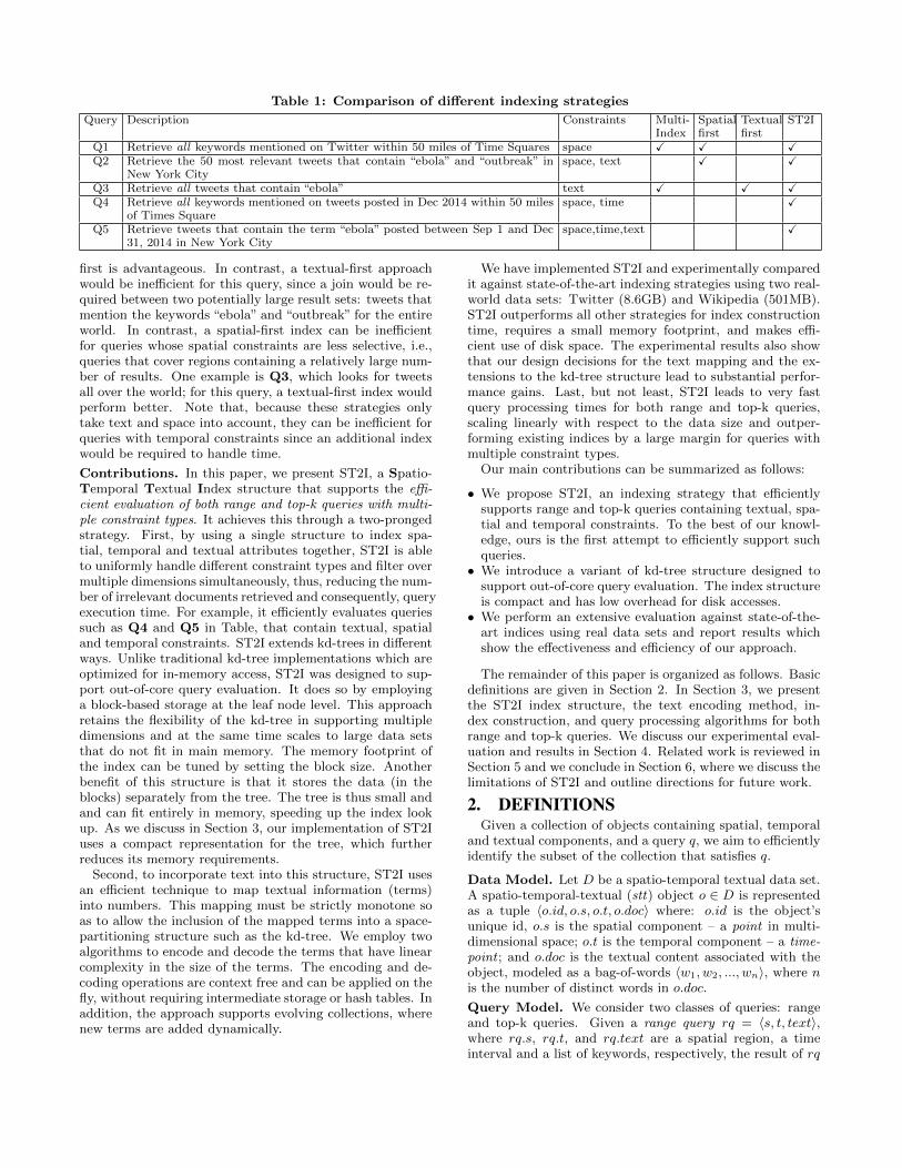
Table 1: Comparison of different indexing strategies

Query Description Constraints Multi-Index

Spatialfirst

Textualfirst

ST2I

Q1 Retrieve all keywords mentioned on Twitter within 50 miles of Time Squares space X X XQ2 Retrieve the 50 most relevant tweets that contain “ebola” and “outbreak” in

New York Cityspace, text X X

Q3 Retrieve all tweets that contain “ebola” text X X XQ4 Retrieve all keywords mentioned on tweets posted in Dec 2014 within 50 miles

of Times Squarespace, time X

Q5 Retrieve tweets that contain the term “ebola” posted between Sep 1 and Dec31, 2014 in New York City

space,time,text X

first is advantageous. In contrast, a textual-first approachwould be inefficient for this query, since a join would be re-quired between two potentially large result sets: tweets thatmention the keywords “ebola” and “outbreak” for the entireworld. In contrast, a spatial-first index can be inefficientfor queries whose spatial constraints are less selective, i.e.,queries that cover regions containing a relatively large num-ber of results. One example is Q3, which looks for tweetsall over the world; for this query, a textual-first index wouldperform better. Note that, because these strategies onlytake text and space into account, they can be inefficient forqueries with temporal constraints since an additional indexwould be required to handle time.

Contributions. In this paper, we present ST2I, a Spatio-Temporal Textual Index structure that supports the effi-cient evaluation of both range and top-k queries with multi-ple constraint types. It achieves this through a two-prongedstrategy. First, by using a single structure to index spa-tial, temporal and textual attributes together, ST2I is ableto uniformly handle different constraint types and filter overmultiple dimensions simultaneously, thus, reducing the num-ber of irrelevant documents retrieved and consequently, queryexecution time. For example, it efficiently evaluates queriessuch as Q4 and Q5 in Table, that contain textual, spatialand temporal constraints. ST2I extends kd-trees in differentways. Unlike traditional kd-tree implementations which areoptimized for in-memory access, ST2I was designed to sup-port out-of-core query evaluation. It does so by employinga block-based storage at the leaf node level. This approachretains the flexibility of the kd-tree in supporting multipledimensions and at the same time scales to large data setsthat do not fit in main memory. The memory footprint ofthe index can be tuned by setting the block size. Anotherbenefit of this structure is that it stores the data (in theblocks) separately from the tree. The tree is thus small andand can fit entirely in memory, speeding up the index lookup. As we discuss in Section 3, our implementation of ST2Iuses a compact representation for the tree, which furtherreduces its memory requirements.

Second, to incorporate text into this structure, ST2I usesan efficient technique to map textual information (terms)into numbers. This mapping must be strictly monotone soas to allow the inclusion of the mapped terms into a space-partitioning structure such as the kd-tree. We employ twoalgorithms to encode and decode the terms that have linearcomplexity in the size of the terms. The encoding and de-coding operations are context free and can be applied on thefly, without requiring intermediate storage or hash tables. Inaddition, the approach supports evolving collections, wherenew terms are added dynamically.

We have implemented ST2I and experimentally comparedit against state-of-the-art indexing strategies using two real-world data sets: Twitter (8.6GB) and Wikipedia (501MB).ST2I outperforms all other strategies for index constructiontime, requires a small memory footprint, and makes effi-cient use of disk space. The experimental results also showthat our design decisions for the text mapping and the ex-tensions to the kd-tree structure lead to substantial perfor-mance gains. Last, but not least, ST2I leads to very fastquery processing times for both range and top-k queries,scaling linearly with respect to the data size and outper-forming existing indices by a large margin for queries withmultiple constraint types.

Our main contributions can be summarized as follows:

• We propose ST2I, an indexing strategy that efficientlysupports range and top-k queries containing textual, spa-tial and temporal constraints. To the best of our knowl-edge, ours is the first attempt to efficiently support suchqueries.• We introduce a variant of kd-tree structure designed to

support out-of-core query evaluation. The index structureis compact and has low overhead for disk accesses.• We perform an extensive evaluation against state-of-the-

art indices using real data sets and report results whichshow the effectiveness and efficiency of our approach.

The remainder of this paper is organized as follows. Basicdefinitions are given in Section 2. In Section 3, we presentthe ST2I index structure, the text encoding method, in-dex construction, and query processing algorithms for bothrange and top-k queries. We discuss our experimental eval-uation and results in Section 4. Related work is reviewed inSection 5 and we conclude in Section 6, where we discuss thelimitations of ST2I and outline directions for future work.

2. DEFINITIONSGiven a collection of objects containing spatial, temporal

and textual components, and a query q, we aim to efficientlyidentify the subset of the collection that satisfies q.

Data Model. Let D be a spatio-temporal textual data set.A spatio-temporal-textual (stt) object o ∈ D is representedas a tuple 〈o.id, o.s, o.t, o.doc〉 where: o.id is the object’sunique id, o.s is the spatial component – a point in multi-dimensional space; o.t is the temporal component – a time-point ; and o.doc is the textual content associated with theobject, modeled as a bag-of-words 〈w1, w2, ..., wn〉, where nis the number of distinct words in o.doc.

Query Model. We consider two classes of queries: rangeand top-k queries. Given a range query rq = 〈s, t, text〉,where rq.s, rq.t, and rq.text are a spatial region, a timeinterval and a list of keywords, respectively, the result of rq

consists of all objects o ∈ D satisfying all constraints (i.e.,o.s ∈ rq.s, o.t ∈ rq.t and o.doc contains all keywords inrq.text). The queries Q1, Q3, Q4 in Table 1 are examplesof range queries.

Instead of retrieving all items that match the query con-straints, a top-k query returns only the k best results basedon a scoring function (e.g., query Q5). A top-k query can berepresented as kq = 〈s, t, text, k〉. Similar to a range queryit has spatial, temporal and textual components, but it alsoincludes one additional parameter k; kq returns k objectso ∈ D ranked according to a distance score.

Scoring for Top-K Queries. The spatial proximity dss(o, q)between an object o and a query q is defined based on thespatial relationship between them:

dss(o, q) = 1− dist(o.s, q.s)

ΓS(1)

where dist(o.s, q.s) is the Euclidean distance between o.s andq.s, and ΓS is the normalization factor, i.e., the maximumEuclidean distance between two points in the dataset D.

The temporal relevance dst(o, q) between object o and aquery q is defined based on their temporal relationship:

dst(o, q) = 1− |o.t− q.t|ΓT

(2)

where ΓT is the normalization factor, i.e., the difference be-tween the smallest and largest time points in D.

The textual relevance dstext(o, q) between object o andquery q is defined based on the query semantics. In thispaper, we consider three cases:

• AND: If q.text ⊂ o.doc (i.e., o.doc must contain all key-words in q.text), dstext(o, q) = 1, otherwise dstext(o, q) =0.• OR: If q.text ∩ o.doc 6= ∅ (i.e., o.doc must contain at

least one keyword in q.text), dstext(o, q) = 1, otherwisedstext(o, q) = 0.• Distance: dstext(o, q) is the distance between o.doc andq.text. Several ranking functions can be employed, suchas the well-known cosine similarity or BM25 [25].

The overall distance score between an object o and a queryq can then be computed by combining the spatial, temporal,and textual distances:

ds(o, q) = α× dss(o, q) +β× dst(o, q) + γ× dstext(o, q) (3)

where α, β and γ are normalization factors that representthe importance of the spatial proximity, temporal and tex-tual relevance, and α + β + γ = 1. These factors are user-defined and input as parameters for each query.

3. INDEXING SPACE, TIME AND TEXTDifferent index structures have been proposed to support

the efficient evaluation of spatial queries. While these struc-tures can be easily extended to support temporal attributes,the same is not true for textual attributes. Here, we proposethe use of a spatial data structure to uniformly handle space,time, and text. We make use of a context-free text map-ping algorithm to encode words into a numeric system, orids, while preserving their alphabetical order (Section 3.1).This allows textual data to be treated as just another nu-merical dimension of the index, enabling it to be efficientlyconstructed and queried in a single pass over the data.

Spatial Data Structures. We considered different choicesfor a spatial index structure, including kd-tree [7], R-tree [18],quadtree [17], and grid index [27]. Quadtree and grid indexquickly become inefficient for large data sets that are notuniformly distributed, especially in high-dimensional spaces.R-tree-based indices (notably R∗-tree [6]) are known fortheir robustness in the presence of data skew and suitabilityfor disk-based query processing. They are widely used in thespatial extensions provided by database systems. However,they have several drawbacks for high-dimensional spaces.Since each index entry needs to store a minimum boundingrectangle (MBR) for all of its child nodes, the size of MBRsgrows linearly as the number of dimensions increases, sodoes the storage requirement. This translates into a smallernumber of indexing entries per block (i.e., the fanout) andreduced efficiency in disk access [36]. The overlapping re-gions among MBRs also grow rapidly with the increase inthe number of dimensions. This can lead to performancedegradation, as more false-positive nodes have to be read [9].While it is possible to optimize R-trees for high-dimensionaldata, i.e., minimizing overlapping regions while maximizingcoverage of MBRs, this problem is non-trivial and computa-tionally expensive. Typically, good splitting strategies [9,18]are quadratic with the number of dimensions, thus makingthe index construction process less scalable.

A kd-tree [7] is a generalization of a binary search treeused to organize points in k dimensional space. Each non-leaf node splits the points in its sub-trees along a hyper-plane. Similar to binary search tree, points to the left ofthe defined hyper-plane are present in the left sub-tree andpoints to the right of the defined hyper-plane are present inthe right sub-tree. The canonical way to select the splittinghyper-plane is to cycle through each dimension, and split atthe median value of that dimension. This allows kd-treesto support simultaneous filtering over multiple dimensionswithout the overlapping and complex partitioning imposedby R-trees. For these reasons, we selected a kd-tree-basedstructure for ST2I. Kd-trees, however, cannot be used toorganize data types such as strings. In what follows, wediscuss how we addressed this problem.

3.1 Indexing TextThe canonical kd-tree supports indexing for geometric

points. In order to index textual data, terms (or keywords)must be encoded as points and the encoding (mapping)method must preserve the alphabetical ordering of the terms.The encoding function f must thus be strictly monotone,i.e., both bijective and monotonic:

• Bijective: For each word w, there exists one and only oneassociated id f(w) and vice versa. This ensures that wecan search every word and that we can map back anyindex result in the numeric space to the textual space.• Monotonic: For each pair of words w1 and w2, if w1 comes

before w2 in the alphabetical order, then id(w1) < id(w2)(e.g., id(apple) < id(apply)). Since our indexing struc-ture relies on numeric comparisons to identify matchingobjects, these comparisons must reflect real textual rela-tions for the index to be meaningful.

A naıve approach would be to extract all distinct terms andsort them before constructing index. Terms can be mappedinto their ranks, and a dictionary can be used during queryevaluation to translate terms in queries into their equiva-lent order. However, this requires a full scan of the data

Algorithm 1: word to id and id to word algorithms

1 // s e t V to alphanumeric cha ra c t e r s2 s t a t i c const char V [ ] =3 ”0123456789 abcdefghi jklmnopqrstuvwxyz ” ;4 // and |V| to the s i z e o f V exc lud ing the5 // nul l−terminated charac t e r at the end6 s t a t i c const i n t nV = s i z e o f ( V )−1;7 s t a t i c const i n t m = 12 ; // max word length8 u in t 64 t word_to_id ( const char ∗ word ) {9 u in t 64 t id=0;

10 f o r ( i n t i=0; word [ i ] && i<m ; ++i )11 id = id∗nV +12 ( ( word [ i ]> ' 9 ' ) ?13 ( word [ i ]− ' a '+10) : // l e t t e r s14 ( word [ i ]− ' 0 ' ) ) ; // numbers15 return id ;16 }17 void id_to_word ( u i n t 64 t id , char ∗ word ) {18 word [ m ] = NULL ;19 f o r ( i n t p=m−1; p>=0 && id ; id/=nV , −−p )20 word [ p ] = V [ id%nV ] ;21 }

and sorting a potentially large number of terms. The sameexpensive process is also required for indexing new terms.

To avoid this inefficiency, we employ two mapping func-tions for encoding and decoding text that can be appliedon the fly. As shown in Algorithm 1, the first algorithm,word to id, does a single scan over an input string and con-verts it into a number using the positional notation method.Its complexity is O(m), where m is a constant representingthe maximum word length. The second algorithm, id to word,is responsible for converting IDs back to words and also hasO(m) complexity. These algorithms are context-free and canbe computed on the fly efficiently without requiring inter-mediate storage or hash tables.

Implementation Details. To design our encoding mecha-nism, we took the following observations into account. Firstof all, words in documents usually have a small number ofcharacters. For instance, the average word length for Englishlanguage is 5.1 [4]. Similar numbers are found in Englishliterature.1 The average word length in the Wikipedia andTwitter data sets used in our experiments is 4.9 and 5.6, re-spectively. Besides, the number of words having more than acertain number of characters follow a power law distribution.As Figure 1 shows, shorter words are more popular thanlonger ones. Secondly, all English words can be expressedby alphanumerics and a limited set of special symbols (e.g.,hashtag (#) and hyphen (-)). Note that this is only a smallsubset of the ASCII standard, and can be encoded usingfewer bits than the usual single-byte representation.

3 4 5 6 7 8 9 10 11 12 13 14 15 16 17 18 19 20Number of characters

0.0

0.2

0.4

0.6

0.8

1.0

Perc

enta

ge

WikipediaTwitter

Figure 1: Power law dis-tribution of word length.

The value of m (12)was carefully chosen so thatthe corresponding numberfor any word of length12 or less containing al-phanumeric characters canbe stored using native 64-bit numbers. Figure 1 showsthat less than one percentof words in Twitter andWikipedia have more than12 characters. Therefore wechoose to encode the first 12 characters of any word insteadof all characters. For example international and interna-tionalization are encoded using the same number. At query

1http://languagelog.ldc.upenn.edu/nll/?p=3532

d = 1 (time)

d = 5 (time)

d = 2 (latitude)

d = 3 (longitude)

d = 4 (keyword)

B

KPointKPointKPoint

KBlocks

KTreeroot

left right

left right left right

left rightleft right

KNode <median, pointer_to_left_child>

Figure 2: Structure of ST2I.

evaluation time, additional word comparisons are requiredto return the correct results. As we discuss in Section 4.3,the overhead for these comparisons is negligible. Note thatthe mapping functions work for English and for languagesthat use Latin characters, but they are not suitable for lan-guages that contain non-latin characters.

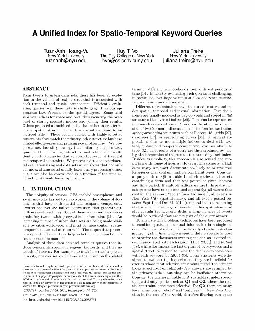
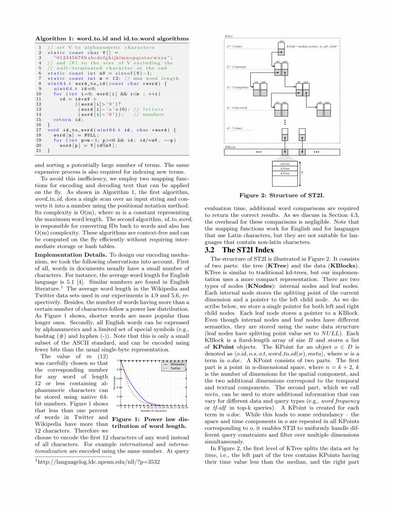
3.2 The ST2I IndexThe structure of ST2I is illustrated in Figure 2. It consists

of two parts: the tree (KTree) and the data (KBlocks).KTree is similar to traditional kd-trees, but our implemen-tation uses a more compact representation. There are twotypes of nodes (KNodes): internal nodes and leaf nodes.Each internal node stores the splitting point of the currentdimension and a pointer to the left child node. As we de-scribe below, we store a single pointer for both left and rightchild nodes. Each leaf node stores a pointer to a KBlock.Even though internal nodes and leaf nodes have differentsemantics, they are stored using the same data structure(leaf nodes have splitting point value set to NULL). EachKBlock is a fixed-length array of size B and stores a listof KPoint objects. The KPoint for an object o ∈ D isdenoted as 〈o.id, o.s, o.t, word to id(w),meta〉, where w is aterm in o.doc. A KPoint consists of two parts. The firstpart is a point in n-dimensional space, where n = k + 2, kis the number of dimensions for the spatial component, andthe two additional dimensions correspond to the temporaland textual components. The second part, which we callmeta, can be used to store additional information that canvary for different data and query types (e.g., word frequencyor tf-idf in top-k queries). A KPoint is created for eachterm in o.doc. While this leads to some redundancy – thespace and time components in o are repeated in all KPointscorresponding to o, it enables ST2I to uniformly handle dif-ferent query constraints and filter over multiple dimensionssimultaneously.

In Figure 2, the first level of KTree splits the data set bytime, i.e., the left part of the tree contains KPoints havingtheir time value less than the median, and the right part

Algorithm 2: st2i build

1 Input: P, root, d23 if |P | ≤ B4 root.content← new Block(P )5 return6 cur d← d mod n % \ label{tc : mod}7 tmp← get value(P, cur d)8 median← nth element(tmp, |P |/2)9 left← 0

10 right← (|P | − 1)11 while left < right12 while get value(P [left], cur d) ≤ median13 left← left + 114 while get value(P [right], cur d) > median15 right← right− 116 if left < right17 swap(P [left], P [right])18 root.median = median19 st2i build(P [0...right], root.left, d + 1)20 st2i build(P [right + 1...|P | − 1], root.left + 1, d + 1)2122 return

of the tree contains KPoints having a value greater than orequal the median. Recursively, the data set is split on thesecond level by latitude, third level by longitude, fourth levelby keyword (using word to id(keyword)), and on the fifthlevel by time again. The process continues until the num-ber of data points being considered is less than the KBlocksize B. In what follows, we discuss the advantages of ST2Icompared to other kd-tree variants [24,26].

Separation of the Tree Structure and Data. Togetherwith using a compact representation (see below), separatingthe tree structure and data leads to a substantial reductionin the size of the KTree. A KTree is usually orders of mag-nitude smaller than the actual data, and thus, it can fit intomemory, allowing efficient traversal of the index. To derivethe answers to a query q, only KBlocks with data relevantto q are accessed.

Compactness of Node Data. ST2I only requires 2 val-ues (integers) per node, compared to 4 values used in [36],and 3 values used in popular libraries like nanoflann [2] andSpatial C++ Library [3]. Since we allocate space for the twochildren of each node in a pair, we only need to store a singlepointer for both of them. This makes the index more com-pact, leading to higher memory locality and faster traversaltime. As a point of reference, storing 2 values instead of 3values saves over 2GB for a 100 million tweets data set (seeSection 4).

Flat Tree Data Structure. We use a single breadth-firstordered array to store the KTree nodes. This is similar tothe storage method used for binary heaps. The root is storedat position 0. A node stored at position i will have its leftchild (if exists) stored at position 2 ∗ i+ 1 and its right childat 2 ∗ i + 2. The array can be simply read sequentially asdeeper levels of KTree are traversed. As we describe below,our KTree construction algorithm stores KNodes in the sameorder as the traversal algorithm accesses them. Combinedwith the fact that non-leaf and leaf nodes use the same datastructure, this method results in a compact storage withhigh-locality of access and low disk overhead.

Use of Memory-Mapped Files. Since ST2I uses a flattree data structure and node size is fixed, the approximatelocation of any node can be calculated efficiently. To supportout-of-core queries seamlessly, in our implementation, wemake use of 64-bit memory-mapped files that are available

Algorithm 3: st2i search

1 Input: q, root2 C ← {}34 if q.t = ∅5 C ← C ∩ st2i traverse(q, root, 0)6 else7 for each w ∈ q.keywords8 idw ← word to id(w)9 qw ← 〈q.p, idw〉

10 C ← C ∩ st2i traverse(qw, root, 0)1112 return st2i process(C)

in current operating systems. By using kernel-space mappedfiles, we avoid making copies of data in user-space and leavethe memory management to the OS.

Complexity. The KTree is balanced: each level of theKTree is split at the median value of each splitting plane,thus the available data points are partitioned equally be-tween the left and right child. Recall that the ST2I usesa block-based storage [26, 28] at the leaf nodes. This is incontrast to the original kd-tree design, where each leaf nodelinks to a single record. This modification allows our datastructure to align better with external memory models. Inaddition, we also use an implicit strategy of dimension in-terleaving to decide which axis to be split at each level. Thebenefits are twofold: this improves worst-case complexity forskewed data sets and reduces the storage cost of the KNodes.Let N be the number of data points and B be the maximumnumber of points per leaf, the maximum depth and the max-imum number of nodes in the KTree are k log(N

B) and N

B,

respectively.In summary, the benefits of ST2I are: (1) since data points

are stored in blocks, it is I/O friendly with a small foot-print; (2) it is cache friendly, because nodes are stored ina breadth-first order array relevant KPoints are likely to beloaded together; and (3) the index structure can be accessedquickly through memory-mapped files leading to increasedperformance and seamless support for disk-based storage.

3.3 Index ConstructionIndex construction is accomplished by two algorithms:

Point Creation and Tree Construction. Point Creation makesa single scan through data set D and converts each spatio-temporal textual object o into a list P of KPoints. Unlikeother approaches, this algorithm requires no prior knowledgeof (or statistics about) the data set. The second algorithm,Tree Construction, uses the list P of KPoints as input andconstructs the KTree. Tree Construction is similar to thecanonical k-d tree construction, but since we use a linearselection algorithm [10] to find the median value for eachsplitting plane, it requires much less time to process eachdimension (O(N) instead of O(N logN)).

The Tree Construction, st2i build (Algorithm 2) receivesas inputs the Point array P , the root node and the depth dof the subtree it is building. It uses two additional parame-ters: n, the number of dimensions (n = k + 2); and B, theKBlock size. The algorithm iterates over the dimensions inthe n-dimensional space. In lines 7 and 8, the keys corre-sponding to the current dimension are extracted and theirmedian value computed. Lines 9 to 17 perform in-placeswappings on P to partition all points around the pivotingmedian point. Lines 19 to 20 recursively construct the leftand right subtrees of the next dimension.

Algorithm 4: st2i traverse

1 Input: q, root, d23 if root.content 6= ∅4 return root.content5 C ← {}6 cur d← d mod n % \ label{tc : mod}7 if (−∞, root.median] ∩ get value(q, cur d) 6= ∅8 C ← C ∩ st2i traverse(q, root.left, d + 1)9 if (root.median,∞) ∩ get value(q, cur d) 6= ∅

10 C ← C ∩ st2i traverse(q, root.left + 1, d + 1)1112 return C

Top-k Query Support. Different from range queries, toprocess top-k queries the algorithm needs to rank each can-didate based on the scoring function. Since the textual rele-vance function requires word frequency, we make use of themeta field of KPoint to store relative frequency of each wordin each object’s document.

Complexity. st2i build works in a divide-and-conquerfashion similar to quicksort, but it always performs balancedpartitioning. For each partition, the complexity is linear,bounded by the selection algorithm and the swapping pro-cess. Let M = N

Bbe the number of leaf nodes in our k-d tree,

the amortized cost of building the index structure at eachdimension would be exactly O(M). Since there is approxi-mately k log(M) levels, the total complexity of st2i buildis O(kM log(M)).

3.4 Query ProcessingSince the spatial, temporal, and textual components of

each object are integrated in the ST2I structure, the queryprocessing algorithm can map any spatio-temporal keywordquery into a range search query regardless of search criteria.To reduce the query processing time, the algorithm readsand navigates the tree in the same order as it stored. Foreach query, ST2I starts from the root of KTree and movesdown recursively, similar to the process used for index con-struction. At each level of the KTree, the algorithm goesleft or right depending on the split value of the current nodeand the value of the query constraint in the current dimen-sion. When a leaf-node is reached, all KPoints in the KBlocklinked from it are added to the candidate list. After the al-gorithm finishes traversing the KTree, each KPoint in thecandidate list is evaluated to check whether it satisfies allquery constraints. The algorithm then outputs the validresults. Evaluation of range queries and top-k queries aredescribed below. For top-k queries, early termination andcandidate ranking strategies are employed to yield betteroverall performance.

Range Query Processing. Single-term and multiple-termqueries are evaluated in a similar fashion. For each keywordw in q.keywords, st2i search (Algorithm 3) converts it intoidw using the word to id algorithm and creates an individ-ual range search query qw from q.s, q.t and idw. Then, foreach qw, st2i search traverses KTree, generates the candi-date KPoints (using Algorithm 4 st2i traverse), and addsthem to the global candidate set C. Finally, depending onthe textual relevance function being used, st2i search ei-ther intersects, unions or calculates the similarity score forcandidates from different keywords, and outputs the finalresults.

Algorithm 4 details the st2i traverse procedure. In ad-dition to the search query q and the current node root,

Algorithm 5: topk st2i search

1 Input: q, root2 outer upperbound← 13 topk lowerbound← 04 cur layer ← 15 TOPK ← {}67 while topk lowerbound < outer upperbound8 cur radius← cur layer × STEP9 update radius of q based on cur radius

10 for each w ∈ q.t11 idw ← word to id(w)12 qw ← 〈q.p, idw〉13 C ← C ∩ st2i traverse(qw, root, 0)14 for each c ∈ C15 compute combined score of c16 append c to TOPK17 update outer upperbound18 update topk lowerbound of TOPK19 cur layer ← cur layer + 12021 return TOPK

st2i traverse also keeps track of the current depth d. Lines 3and 4 check if a leaf-node has been reached. If so, all pointsin the linked block are returned as candidates. Otherwise,lines 7 to 10 compare the value of the current node (i.e.,root.median) with the value for the query constraint in thesplit dimension cur d, and recursively traverse left, right orboth, until a leaf-node is reached.

Top-k Query Processing. The key idea behind the opti-mization techniques for spatial top-k queries is to partitionthe search space into layers relative to the position specifiedin the search query. Then, the algorithm only retrieves andvalidates candidates one layer at a time, thus avoiding com-putation and validation for answers not among the top-k.For each layer, we need to compute the lower bound of thetop-k candidate list and the upper bound of all other pointsoutside of the layer. The algorithm stops when the lowerbound from the top-k is larger than the upper bound of theremaining points.

In Algorithm 5, we present a variant of st2i search calledtopk st2i search to support top-k queries. TOPK is a pri-ority queue that stores the current best q.k objects as well asthe upper bounds and lower bounds of its members. In eachiteration, topk st2i search expands the current search ra-dius by STEP – the unit size of the divided spatial layers.Assuming that the spatial search space is divided into η lay-ers (i.e., it takes η iterations to go over all points in the

search space), STEP = ΓSη

. Then for each keyword in thequery, topk st2i search traverses through the KTree andyields candidate list. The score for each candidate c is cal-culated by a scoring function and the pair 〈c, score(c)〉 isadded to TOPK. At the end of each iteration, the lowerbound of TOPK and the upper bound of the outer layerare updated. The upper bound of outer layer is calculatedbased on the upper bound of the spatial proximity, temporalrelevance and textual relevance as follows:

outer upperbound = α×(1− cur radiusΓS

)+β×1+γ×1 (4)

where α× (1− cur radiusΓS

) is the maximum score of any ob-

jects in the next layer; β×1 and γ×1 are the maximum pos-sible temporal relevance and textual relevance, respectively.The algorithm terminates when the maximum possible scoreof any object in the outer layer is smaller than the minimumscore of all elements in TOPK.

20 40 60 80 100Dataset size (in million tweets)

100

101

102

103

104

105

Build

ing T

ime (

in m

inute

s) RCA

ST2I

Lucene

SFC-QUAD

(a) Building time (log scale)

20 40 60 80 100Dataset size (in million tweets)

100

101

102

103

Mem

ory

footp

rint

(in G

B) RCA

ST2I

Lucene

SFC-QUAD

(b) Memory footprint (log scale)

20 40 60 80 100Dataset size (in million tweets)

0

10

20

30

40

50

60

Dis

k sp

ace

(in

GB

)

ST2I

RCA

Lucene

SFC-QUAD

(c) Disk space

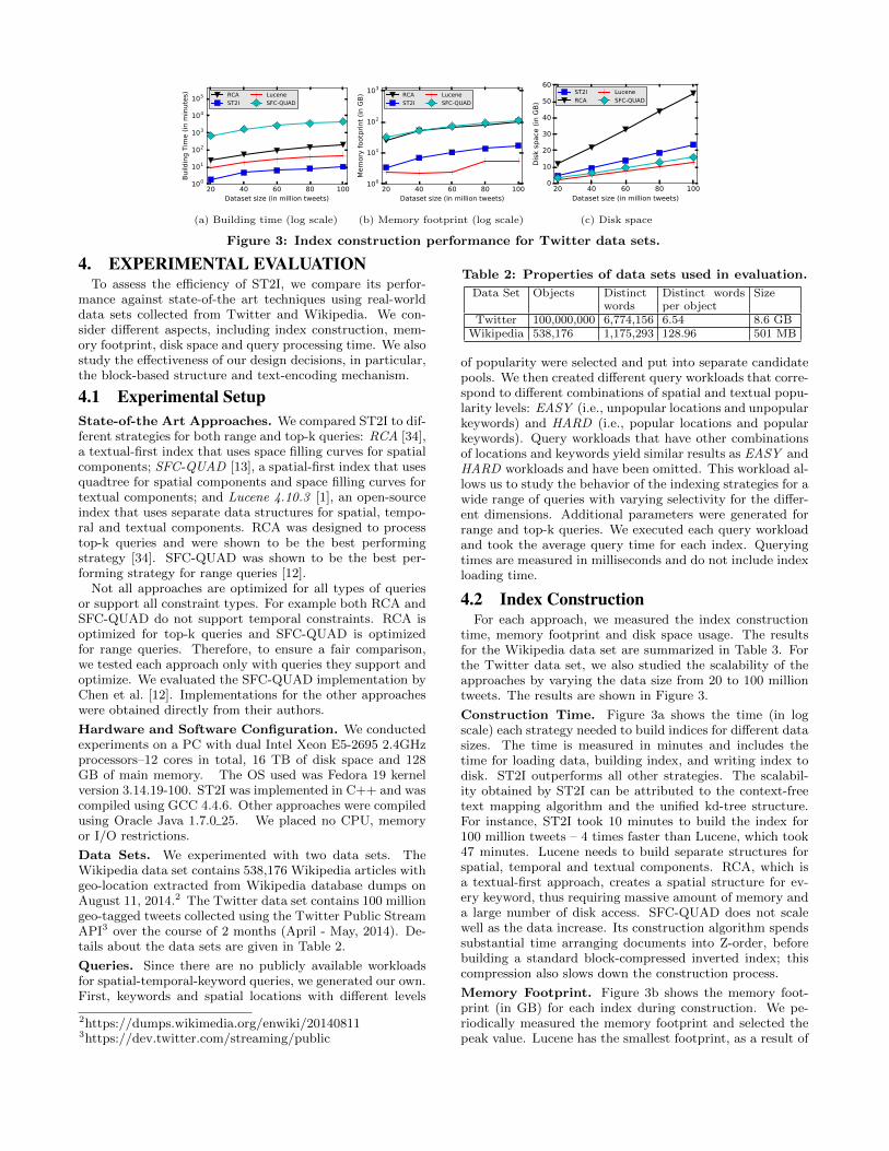
Figure 3: Index construction performance for Twitter data sets.

4. EXPERIMENTAL EVALUATIONTo assess the efficiency of ST2I, we compare its perfor-

mance against state-of-the art techniques using real-worlddata sets collected from Twitter and Wikipedia. We con-sider different aspects, including index construction, mem-ory footprint, disk space and query processing time. We alsostudy the effectiveness of our design decisions, in particular,the block-based structure and text-encoding mechanism.

4.1 Experimental SetupState-of-the Art Approaches. We compared ST2I to dif-ferent strategies for both range and top-k queries: RCA [34],a textual-first index that uses space filling curves for spatialcomponents; SFC-QUAD [13], a spatial-first index that usesquadtree for spatial components and space filling curves fortextual components; and Lucene 4.10.3 [1], an open-sourceindex that uses separate data structures for spatial, tempo-ral and textual components. RCA was designed to processtop-k queries and were shown to be the best performingstrategy [34]. SFC-QUAD was shown to be the best per-forming strategy for range queries [12].

Not all approaches are optimized for all types of queriesor support all constraint types. For example both RCA andSFC-QUAD do not support temporal constraints. RCA isoptimized for top-k queries and SFC-QUAD is optimizedfor range queries. Therefore, to ensure a fair comparison,we tested each approach only with queries they support andoptimize. We evaluated the SFC-QUAD implementation byChen et al. [12]. Implementations for the other approacheswere obtained directly from their authors.

Hardware and Software Configuration. We conductedexperiments on a PC with dual Intel Xeon E5-2695 2.4GHzprocessors–12 cores in total, 16 TB of disk space and 128GB of main memory. The OS used was Fedora 19 kernelversion 3.14.19-100. ST2I was implemented in C++ and wascompiled using GCC 4.4.6. Other approaches were compiledusing Oracle Java 1.7.0 25. We placed no CPU, memoryor I/O restrictions.

Data Sets. We experimented with two data sets. TheWikipedia data set contains 538,176 Wikipedia articles withgeo-location extracted from Wikipedia database dumps onAugust 11, 2014.2 The Twitter data set contains 100 milliongeo-tagged tweets collected using the Twitter Public StreamAPI3 over the course of 2 months (April - May, 2014). De-tails about the data sets are given in Table 2.

Queries. Since there are no publicly available workloadsfor spatial-temporal-keyword queries, we generated our own.First, keywords and spatial locations with different levels

2https://dumps.wikimedia.org/enwiki/201408113https://dev.twitter.com/streaming/public

Table 2: Properties of data sets used in evaluation.

Data Set Objects Distinctwords

Distinct wordsper object

Size

Twitter 100,000,000 6,774,156 6.54 8.6 GBWikipedia 538,176 1,175,293 128.96 501 MB

of popularity were selected and put into separate candidatepools. We then created different query workloads that corre-spond to different combinations of spatial and textual popu-larity levels: EASY (i.e., unpopular locations and unpopularkeywords) and HARD (i.e., popular locations and popularkeywords). Query workloads that have other combinationsof locations and keywords yield similar results as EASY andHARD workloads and have been omitted. This workload al-lows us to study the behavior of the indexing strategies for awide range of queries with varying selectivity for the differ-ent dimensions. Additional parameters were generated forrange and top-k queries. We executed each query workloadand took the average query time for each index. Queryingtimes are measured in milliseconds and do not include indexloading time.

4.2 Index ConstructionFor each approach, we measured the index construction

time, memory footprint and disk space usage. The resultsfor the Wikipedia data set are summarized in Table 3. Forthe Twitter data set, we also studied the scalability of theapproaches by varying the data size from 20 to 100 milliontweets. The results are shown in Figure 3.

Construction Time. Figure 3a shows the time (in logscale) each strategy needed to build indices for different datasizes. The time is measured in minutes and includes thetime for loading data, building index, and writing index todisk. ST2I outperforms all other strategies. The scalabil-ity obtained by ST2I can be attributed to the context-freetext mapping algorithm and the unified kd-tree structure.For instance, ST2I took 10 minutes to build the index for100 million tweets – 4 times faster than Lucene, which took47 minutes. Lucene needs to build separate structures forspatial, temporal and textual components. RCA, which isa textual-first approach, creates a spatial structure for ev-ery keyword, thus requiring massive amount of memory anda large number of disk access. SFC-QUAD does not scalewell as the data increase. Its construction algorithm spendssubstantial time arranging documents into Z-order, beforebuilding a standard block-compressed inverted index; thiscompression also slows down the construction process.

Memory Footprint. Figure 3b shows the memory foot-print (in GB) for each index during construction. We pe-riodically measured the memory footprint and selected thepeak value. Lucene has the smallest footprint, as a result of

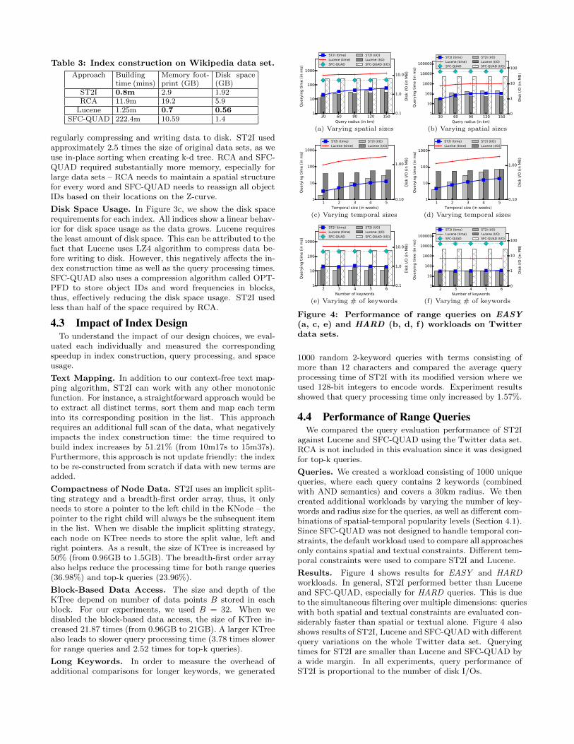
Table 3: Index construction on Wikipedia data set.

Approach Buildingtime (mins)

Memory foot-print (GB)

Disk space(GB)

ST2I 0.8m 2.9 1.92RCA 11.9m 19.2 5.9

Lucene 1.25m 0.7 0.56SFC-QUAD 222.4m 10.59 1.4

regularly compressing and writing data to disk. ST2I usedapproximately 2.5 times the size of original data sets, as weuse in-place sorting when creating k-d tree. RCA and SFC-QUAD required substantially more memory, especially forlarge data sets – RCA needs to maintain a spatial structurefor every word and SFC-QUAD needs to reassign all objectIDs based on their locations on the Z-curve.

Disk Space Usage. In Figure 3c, we show the disk spacerequirements for each index. All indices show a linear behav-ior for disk space usage as the data grows. Lucene requiresthe least amount of disk space. This can be attributed to thefact that Lucene uses LZ4 algorithm to compress data be-fore writing to disk. However, this negatively affects the in-dex construction time as well as the query processing times.SFC-QUAD also uses a compression algorithm called OPT-PFD to store object IDs and word frequencies in blocks,thus, effectively reducing the disk space usage. ST2I usedless than half of the space required by RCA.

4.3 Impact of Index DesignTo understand the impact of our design choices, we eval-

uated each individually and measured the correspondingspeedup in index construction, query processing, and spaceusage.

Text Mapping. In addition to our context-free text map-ping algorithm, ST2I can work with any other monotonicfunction. For instance, a straightforward approach would beto extract all distinct terms, sort them and map each terminto its corresponding position in the list. This approachrequires an additional full scan of the data, what negativelyimpacts the index construction time: the time required tobuild index increases by 51.21% (from 10m17s to 15m37s).Furthermore, this approach is not update friendly: the indexto be re-constructed from scratch if data with new terms areadded.

Compactness of Node Data. ST2I uses an implicit split-ting strategy and a breadth-first order array, thus, it onlyneeds to store a pointer to the left child in the KNode – thepointer to the right child will always be the subsequent itemin the list. When we disable the implicit splitting strategy,each node on KTree needs to store the split value, left andright pointers. As a result, the size of KTree is increased by50% (from 0.96GB to 1.5GB). The breadth-first order arrayalso helps reduce the processing time for both range queries(36.98%) and top-k queries (23.96%).

Block-Based Data Access. The size and depth of theKTree depend on number of data points B stored in eachblock. For our experiments, we used B = 32. When wedisabled the block-based data access, the size of KTree in-creased 21.87 times (from 0.96GB to 21GB). A larger KTreealso leads to slower query processing time (3.78 times slowerfor range queries and 2.52 times for top-k queries).

Long Keywords. In order to measure the overhead ofadditional comparisons for longer keywords, we generated

0.1

1.0

10.0

Dis

k I/O

(in

MB

)

30 60 90 120 150Query radius (in km)

1

10

100

1000

Query

ing t

ime (

in m

s)

ST2I (time)

Lucene (time)

SFC-QUAD

ST2I (I/O)

Lucene (I/O)

SFC-QUAD (I/O)

(a) Varying spatial sizes

0

1

10

100

Dis

k I/O

(in

MB

)

30 60 90 120 150Query radius (in km)

1

10

100

1000

10000

100000

Query

ing t

ime (

in m

s)

ST2I (time)

Lucene (time)

SFC-QUAD

ST2I (I/O)

Lucene (I/O)

SFC-QUAD (I/O)

(b) Varying spatial sizes

0.10

1.00

Dis

k I/O

(in

MB

)

1 2 3 4 5Temporal size (in weeks)

1

10

100

1000

Query

ing t

ime (

in m

s)

ST2I (time)

Lucene (time)

ST2I (I/O)

Lucene (I/O)

(c) Varying temporal sizes

0.10

1.00

Dis

k I/O

(in

MB

)

1 2 3 4 5Temporal size (in weeks)

1

10

100

1000

Query

ing t

ime (

in m

s)

ST2I (time)

Lucene (time)

ST2I (I/O)

Lucene (I/O)

(d) Varying temporal sizes

0.1

1.0

10.0

Dis

k I/O

(in

MB

)

2 3 4 5 6Number of keywords

1

10

100

1000

Query

ing t

ime (

in m

s)

ST2I (time)

Lucene (time)

SFC-QUAD

ST2I (I/O)

Lucene (I/O)

SFC-QUAD (I/O)

(e) Varying # of keywords

0

1

10

100

Dis

k I/O

(in

MB

)

2 3 4 5 6Number of keywords

1

10

100

1000

10000

100000

Query

ing t

ime (

in m

s)

ST2I (time)

Lucene (time)

SFC-QUAD

ST2I (I/O)

Lucene (I/O)

SFC-QUAD (I/O)

(f) Varying # of keywords

Figure 4: Performance of range queries on EASY(a, c, e) and HARD (b, d, f) workloads on Twitterdata sets.

1000 random 2-keyword queries with terms consisting ofmore than 12 characters and compared the average queryprocessing time of ST2I with its modified version where weused 128-bit integers to encode words. Experiment resultsshowed that query processing time only increased by 1.57%.

4.4 Performance of Range QueriesWe compared the query evaluation performance of ST2I

against Lucene and SFC-QUAD using the Twitter data set.RCA is not included in this evaluation since it was designedfor top-k queries.

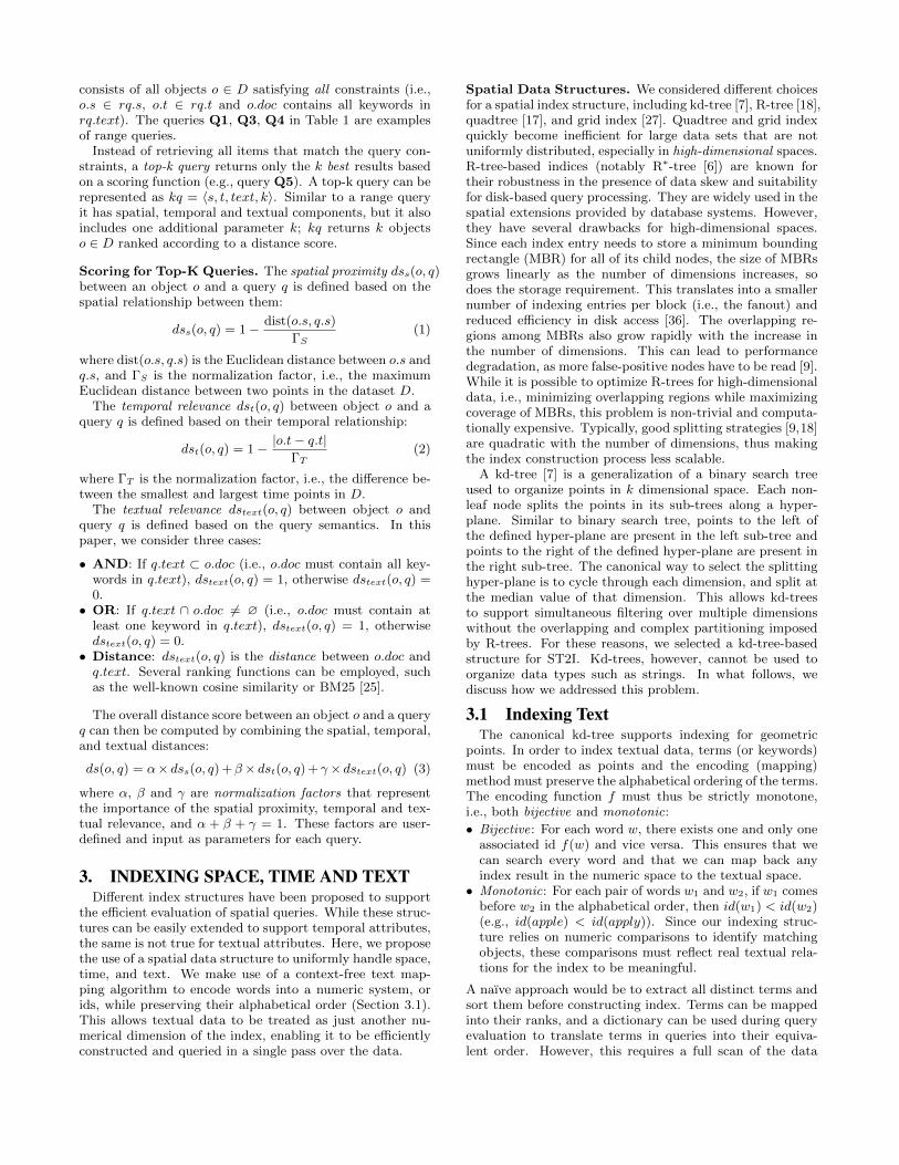
Queries. We created a workload consisting of 1000 uniquequeries, where each query contains 2 keywords (combinedwith AND semantics) and covers a 30km radius. We thencreated additional workloads by varying the number of key-words and radius size for the queries, as well as different com-binations of spatial-temporal popularity levels (Section 4.1).Since SFC-QUAD was not designed to handle temporal con-straints, the default workload used to compare all approachesonly contains spatial and textual constraints. Different tem-poral constraints were used to compare ST2I and Lucene.

Results. Figure 4 shows results for EASY and HARDworkloads. In general, ST2I performed better than Luceneand SFC-QUAD, especially for HARD queries. This is dueto the simultaneous filtering over multiple dimensions: querieswith both spatial and textual constraints are evaluated con-siderably faster than spatial or textual alone. Figure 4 alsoshows results of ST2I, Lucene and SFC-QUAD with differentquery variations on the whole Twitter data set. Queryingtimes for ST2I are smaller than Lucene and SFC-QUAD bya wide margin. In all experiments, query performance ofST2I is proportional to the number of disk I/Os.

0

2

4

6

8

10

12

14

16

Dis

k I/O

(in

GB

)

50 100 150 200 250Number of results (k)

101

102

103

104

Query

ing t

ime (

in m

s)ST2I

RCA

Lucene

ST2I (I/O)

RCA (I/O)

Lucene (I/O)

(a) Varying k

0

5

10

15

20

Dis

k I/O

(in

GB

)

50 100 150 200 250Number of results (k)

101

102

103

104

105

106

Query

ing t

ime (

in m

s)

ST2I

RCA

Lucene

ST2I (I/O)

RCA (I/O)

Lucene (I/O)

(b) Varying k

0

2

4

6

8

10

12

14

16

Dis

k I/O

(in

GB

)

2 3 4 5 6Number of keywords

101

102

103

104

105

Query

ing t

ime (

in m

s)

ST2I

RCA

Lucene

ST2I (I/O)

RCA (I/O)

Lucene (I/O)

(c) Varying # of keywords

0

5

10

15

20

Dis

k I/O

(in

GB

)

2 3 4 5 6Number of keywords

101

102

103

104

105

106

Query

ing t

ime (

in m

s)

ST2I

RCA

Lucene

ST2I (I/O)

RCA (I/O)

Lucene (I/O)

(d) Varying # of keywords

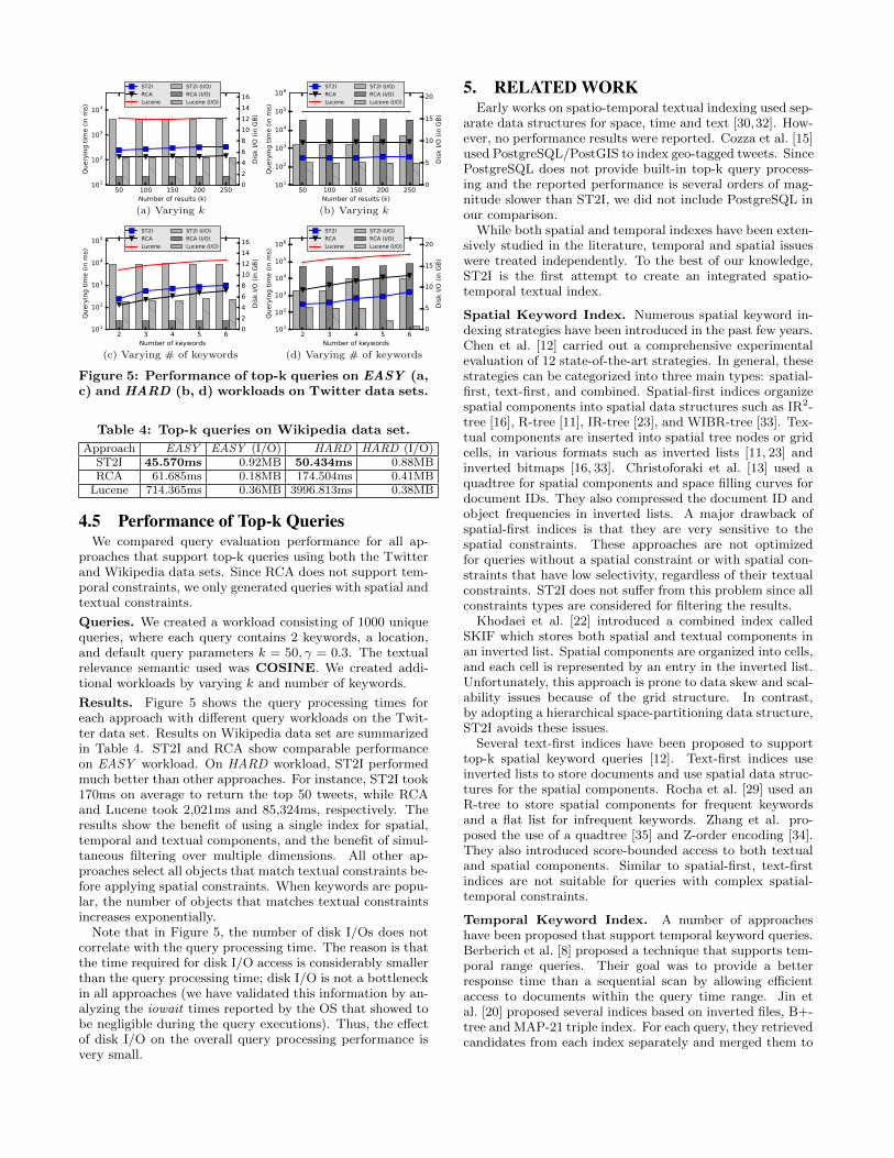
Figure 5: Performance of top-k queries on EASY (a,c) and HARD (b, d) workloads on Twitter data sets.

Table 4: Top-k queries on Wikipedia data set.

Approach EASY EASY (I/O) HARD HARD (I/O)ST2I 45.570ms 0.92MB 50.434ms 0.88MBRCA 61.685ms 0.18MB 174.504ms 0.41MB

Lucene 714.365ms 0.36MB 3996.813ms 0.38MB

4.5 Performance of Top-k QueriesWe compared query evaluation performance for all ap-

proaches that support top-k queries using both the Twitterand Wikipedia data sets. Since RCA does not support tem-poral constraints, we only generated queries with spatial andtextual constraints.

Queries. We created a workload consisting of 1000 uniquequeries, where each query contains 2 keywords, a location,and default query parameters k = 50, γ = 0.3. The textualrelevance semantic used was COSINE. We created addi-tional workloads by varying k and number of keywords.

Results. Figure 5 shows the query processing times foreach approach with different query workloads on the Twit-ter data set. Results on Wikipedia data set are summarizedin Table 4. ST2I and RCA show comparable performanceon EASY workload. On HARD workload, ST2I performedmuch better than other approaches. For instance, ST2I took170ms on average to return the top 50 tweets, while RCAand Lucene took 2,021ms and 85,324ms, respectively. Theresults show the benefit of using a single index for spatial,temporal and textual components, and the benefit of simul-taneous filtering over multiple dimensions. All other ap-proaches select all objects that match textual constraints be-fore applying spatial constraints. When keywords are popu-lar, the number of objects that matches textual constraintsincreases exponentially.

Note that in Figure 5, the number of disk I/Os does notcorrelate with the query processing time. The reason is thatthe time required for disk I/O access is considerably smallerthan the query processing time; disk I/O is not a bottleneckin all approaches (we have validated this information by an-alyzing the iowait times reported by the OS that showed tobe negligible during the query executions). Thus, the effectof disk I/O on the overall query processing performance isvery small.

5. RELATED WORKEarly works on spatio-temporal textual indexing used sep-

arate data structures for space, time and text [30,32]. How-ever, no performance results were reported. Cozza et al. [15]used PostgreSQL/PostGIS to index geo-tagged tweets. SincePostgreSQL does not provide built-in top-k query process-ing and the reported performance is several orders of mag-nitude slower than ST2I, we did not include PostgreSQL inour comparison.

While both spatial and temporal indexes have been exten-sively studied in the literature, temporal and spatial issueswere treated independently. To the best of our knowledge,ST2I is the first attempt to create an integrated spatio-temporal textual index.

Spatial Keyword Index. Numerous spatial keyword in-dexing strategies have been introduced in the past few years.Chen et al. [12] carried out a comprehensive experimentalevaluation of 12 state-of-the-art strategies. In general, thesestrategies can be categorized into three main types: spatial-first, text-first, and combined. Spatial-first indices organizespatial components into spatial data structures such as IR2-tree [16], R-tree [11], IR-tree [23], and WIBR-tree [33]. Tex-tual components are inserted into spatial tree nodes or gridcells, in various formats such as inverted lists [11, 23] andinverted bitmaps [16, 33]. Christoforaki et al. [13] used aquadtree for spatial components and space filling curves fordocument IDs. They also compressed the document ID andobject frequencies in inverted lists. A major drawback ofspatial-first indices is that they are very sensitive to thespatial constraints. These approaches are not optimizedfor queries without a spatial constraint or with spatial con-straints that have low selectivity, regardless of their textualconstraints. ST2I does not suffer from this problem since allconstraints types are considered for filtering the results.

Khodaei et al. [22] introduced a combined index calledSKIF which stores both spatial and textual components inan inverted list. Spatial components are organized into cells,and each cell is represented by an entry in the inverted list.Unfortunately, this approach is prone to data skew and scal-ability issues because of the grid structure. In contrast,by adopting a hierarchical space-partitioning data structure,ST2I avoids these issues.

Several text-first indices have been proposed to supporttop-k spatial keyword queries [12]. Text-first indices useinverted lists to store documents and use spatial data struc-tures for the spatial components. Rocha et al. [29] used anR-tree to store spatial components for frequent keywordsand a flat list for infrequent keywords. Zhang et al. pro-posed the use of a quadtree [35] and Z-order encoding [34].They also introduced score-bounded access to both textualand spatial components. Similar to spatial-first, text-firstindices are not suitable for queries with complex spatial-temporal constraints.

Temporal Keyword Index. A number of approacheshave been proposed that support temporal keyword queries.Berberich et al. [8] proposed a technique that supports tem-poral range queries. Their goal was to provide a betterresponse time than a sequential scan by allowing efficientaccess to documents within the query time range. Jin etal. [20] proposed several indices based on inverted files, B+-tree and MAP-21 triple index. For each query, they retrievedcandidates from each index separately and merged them to

produce final results. However none of their ranking func-tions took into account the temporal relevance score.

Khodaei et al. [21] proposed a temporal-textual indexstructure called T2I2 that combines both temporal and tex-tual components into an inverted list. Textual componentsare organized into cells and each cell is represented by anentry in the inverted list. As with any grid structure, thisapproach is also prone to data skew besides having a largestorage requirement. He et al. [19] introduced methods toprovide better support for querying over versioned docu-ments. They studied different partitioning methods to orga-nize documents by time. It is not clear how these specializedindices can efficiently support spatial constraints.

6. CONCLUSIONSIn this paper, we introduced ST2I, a new indexing strat-

egy that uniformly handles text, space and time in a singlestructure. ST2I uses context-free text mapping algorithmsto encode words in text as numbers, and a block-based kd-tree structure embedded in a breadth-first order layout thathas a space requirement up to 50% smaller than currenttechniques. This effectively increases the memory locality,leading to better querying performance and enabling largerdata sets to be indexed. The flat memory structure also al-lows us to take advantage of 64-bit memory mapped files tosignificantly reduce overhead for serving queries from disks.Our experimental results show that ST2I performs uniformlybetter than the other approaches: it is substantially fasterfor both index construction and query evaluation, and italso has smaller memory footprints and storage requirementsthan most approaches.

In future work, we intend to improve performance of ST2Iby exploiting the parallelism supported by multiple CPUcores, exploring efficient update approaches and develop-ing a variable-bitrate encoding to support longer terms andlarger character set.

Acknowledgments. This work was supported in part byNSF award CNS-1229185 and DARPA award FA8750-14-2-023. Opinions, findings and conclusions expressed in thismaterial are those of the authors and do not necessarilyreflect the views of the NSF or DARPA.

7. REFERENCES[1] Lucene. http://lucene.apache.org, 2014.

[2] nanoflann: Approximate Nearest Neighbor.https://code.google.com/p/nanoflann/, 2014.

[3] Spatial C++ Library. http://spatial.sourceforge.net, 2014.[4] WolframAlpha. http://www.wolframalpha.com/input/?i=

average+english+word+length, 2014.[5] L. Barbosa, K. Pham, C. Silva, M. R. Vieira, and J. Freire.

Structured Open Urban Data: Understanding theLandscape. Big Data, pages 144–154, 2014.

[6] N. Beckmann, H.-P. Kriegel, R. Schneider, and B. Seeger.The R*-tree: An Efficient and Robust Access Method forPoints and Rectangles. In SIGMOD, pages 322–331, 1990.

[7] J. L. Bentley. Multidimensional Binary Search Trees Usedfor Associative Searching. CACM, pages 509–517, 1975.

[8] K. Berberich, S. Bedathur, T. Neumann, and G. Weikum.A Time Machine for Text Search. In SIGIR, 2007.

[9] S. Berchtold, D. A. Keim, and H.-P. Kriegel. The X-tree:An Index Structure for High-Dimensional Data. In VLDB,pages 28–39, 1996.

[10] M. Blum, R. W. Floyd, V. Pratt, R. L. Rivest, and R. E.Tarjan. Time Bounds for Selection. J. Comput. Syst. Sci.,pages 448–461, 1973.

[11] A. Cary, O. Wolfson, and N. Rishe. Efficient and ScalableMethod for Processing Top-k Spatial Boolean Queries. InSSDBM, volume 6187, pages 87–95. 2010.

[12] L. Chen, G. Cong, C. S. Jensen, and D. Wu. SpatialKeyword Query Processing: An Experimental Evaluation.PVLDB, pages 217–228, 2013.

[13] M. Christoforaki, J. He, C. Dimopoulos, A. Markowetz, andT. Suel. Text vs. Space: Efficient Geo-search QueryProcessing. In CIKM, pages 423–432, 2011.

[14] R. Chunara, J. Andrews, and J. Brownstein. Social andnews media enable estimation of epidemiological patternsearly in the 2010 haitian cholera outbreak. AJTMH, 2012.

[15] V. Cozza, A. Messina, D. Montesi, L. Arietta, andM. Magnani. Spatio-temporal keyword queries in socialnetworks. In ADBIS, volume 8133, pages 70–83. 2013.

[16] I. De Felipe, V. Hristidis, and N. Rishe. Keyword Search onSpatial Databases. In ICDE, pages 656–665, 2008.

[17] R. Finkel and J. Bentley. Quad trees a data structure forretrieval on composite keys. Acta Informatica, 1974.

[18] A. Guttman. R-trees: A Dynamic Index Structure forSpatial Searching. In SIGMOD, pages 47–57, 1984.

[19] J. He and T. Suel. Faster temporal range queries overversioned text. In SIGIR, pages 565–574, 2011.

[20] P. Jin, H. Chen, X. Zhao, X. Li, and L. Yue. Indexingtemporal information for web pages. ComSIS, 2011.

[21] A. Khodaei, C. Shahabi, and A. Khodaei.Temporal-Textual Retrieval: Time and Keyword Search inWeb Documents. IJNGC, 2012.

[22] A. Khodaei, C. Shahabi, and C. Li. Hybrid indexing andseamless ranking of spatial and textual features of webdocuments. In DEXA, pages 450–466. 2010.

[23] Z. Li, K. Lee, B. Zheng, W.-C. Lee, D. L. Lee, andX. Wang. IR-Tree: An Efficient Index for GeographicDocument Search. TKDE, pages 585–599, 2011.

[24] D. B. Lomet and B. Salzberg. The hB-tree: AMultiattribute Indexing Method with Good GuaranteedPerformance. TODS, pages 625–658, 1990.

[25] C. D. Manning, P. Raghavan, and H. Schutze. Introductionto information retrieval, volume 1. Cambridge UniversityPress, 2008.

[26] O. Procopiuc, P. Agarwal, L. Arge, and J. Vitter.Bkd-Tree: A Dynamic Scalable kd-Tree. In SSTD, volume2750, pages 46–65. 2003.

[27] P. Rigaux, M. Scholl, and A. Voisard. Spatial Databaseswith Application to GIS. Morgan Kaufmann PublishersInc., 2002.

[28] J. T. Robinson. The K-D-B-tree: A Search Structure forLarge Multidimensional Dynamic Indexes. In SIGMOD,pages 10–18, 1981.

[29] J. a. B. Rocha-Junior, O. Gkorgkas, S. Jonassen, andK. Nørvag. Efficient Processing of Top-k Spatial KeywordQueries. In SSTD, pages 205–222, 2011.

[30] J. Strotgen and M. Gertz. TimeTrails: A System forExploring Spatio-temporal Information in Documents.PVLDB, pages 1569–1572, 2010.

[31] Twitter. https://about.twitter.com/company, 2014.[32] B. Wang, H. Dong, A. P. Boedihardjo, C.-T. Lu, H. Yu,

I.-R. Chen, and J. Dai. An Integrated Framework forSpatio-temporal-textual Search and Mining. InSIGSPATIAL, pages 570–573, 2012.

[33] D. Wu, M. L. Yiu, G. Cong, and C. S. Jensen. Joint Top-KSpatial Keyword Query Processing. TKDE, 2012.

[34] D. Zhang, C.-Y. Chan, and K.-L. Tan. Processing SpatialKeyword Query As a Top-k Aggregation Query. In SIGIR,pages 355–364, 2014.

[35] D. Zhang, K.-L. Tan, and A. K. H. Tung. Scalable Top-kSpatial Keyword Search. In EDBT, pages 359–370, 2013.

[36] P. Zhou and B. Salzberg. The hB-pi* Tree: An OptimizedComprehensive Access Method for Frequent-UpdateMulti-dimensional Point Data. In SSDBM, 2008.