A Unified Approach to Scheduling on Unrelated Parallel Machines∗

V. S. Anil Kumar† Madhav V. Marathe‡ Srinivasan Parthasarathy§

Aravind Srinivasan¶

Abstract

We develop a single rounding algorithm for scheduling on unrelated parallel machines; this algorithmworks well with the known linear programming-, quadratic programming-, and convex programming-relaxations for scheduling to minimize completion time, makespan, and other well-studied objectivefunctions. This algorithm leads to the following applications for the general setting of unrelated parallelmachines: (i) a bicriteria algorithm for a schedule whose weighted completion-time and makespan si-multaneously exhibit the current-best individual approximations for these criteria; (ii) better-than-twoapproximation guarantees for scheduling to minimize the Lp norm of the vector of machine-loads, forall 1 < p <∞; and (iii) the first constant-factor multicriteria approximation algorithms that can handlethe weighted completion-time and any given collection of integer Lp norms. Our algorithm has a naturalinterpretation as a melding of linear-algebraic and probabilistic approaches. Via this view, it yields acommon generalization of rounding theorems due to Karp et al. and Shmoys & Tardos, and leads toimproved approximation algorithms for the problem of scheduling with resource-dependent processingtimes introduced by Grigoriev et al.

1 Introduction

The complexity and approximability of scheduling problems for multiple machines is an area of activeresearch [17, 20]. A particularly general (and challenging) case involves scheduling on unrelated parallelmachines, where the processing times of jobs depend arbitrarily on the machines to which they are assigned.That is, we are given n jobs and m machines, and each job needs to be scheduled on exactly one machine;we are also given a collection of integer values pi,j such that if we schedule job j on machine i, then theprocessing time of operation j is pi,j . Three major objective functions, all NP -hard, in this context areto minimize the weighted completion-time of the jobs, the Lp norm of the loads on the machines, and themaximum completion-time of the machines, or the makespan (i.e., the L∞ norm of the machine-loads)[18, 21, 22, 4]. There is no single measure that is considered “universally good”, and therefore there hasbeen much interest in simultaneously optimizing many given objective functions: if there is a schedule thatsimultaneously has cost Ti with respect to objective i for each i, we aim to efficiently construct a schedulethat has cost λiTi for the ith objective, for each i. (One typical goal here is to keep all the λi small.) The

∗A preliminary version of this paper appeared as the paper “Approximation Algorithms for Scheduling on Multiple Ma-chines”, in the Proc. IEEE Symposium on Foundations of Computer Science, pages 254–263, 2005.

†Department of Computer Science, Virginia Tech, Blacksburg 24061. Email: akumar@vbi.vt.edu‡Virginia Bio-informatics Institute and Department of Computer Science, Virginia Tech, Blacksburg 24061. Email:

mmarathe@vbi.vt.edu§IBM T. J. Watson Research Center, 19, Skyline Drive, Hawthorne, NY 10532. Work done while at the Department of

Computer Science, University of Maryland, College Park, MD 20742. Email: spartha@us.ibm.com¶Department of Computer Science and Institute for Advanced Computer Studies, University of Maryland, College Park,

MD 20742. Email: srin@cs.umd.edu

1

current-best approximation algorithms for these measures are very much tailored to the individual measure.We develop a unified approach to all of these problems, leading to better approximation algorithms for thesingle-criterion and multi-criteria versions.

We will primarily focus on approximation algorithms, since all problems considered herein are NP -hard. Most of the current approaches for these single-criterion or multi-criteria problems are based onconstructing fractional solutions by different linear programming (LP)-, quadratic programming-, andconvex programming-relaxations and then rounding them into integral solutions. Two major roundingapproaches for these problems are those of Lenstra, Shmoys & Tardos and Shmoys & Tardos [18, 21], andclassical randomized rounding (Raghavan & Thompson [19]) as applied to specific problems by Skutella[22] and Azar & Epstein [4]. We develop a single rounding technique that works with all of these relax-ations, gives improved bounds for scheduling under the Lp norms, and most importantly, helps developschedules that are good for multiple combinations of the completion-time and Lp-norm criteria. For thecase of simultaneous weighted completion time and makespan objectives, our approach yields a bicriteriaapproximation with the best-known guarantees for both these objectives. We start by presenting four ofour applications, and then discuss our rounding technique and other implications thereof.

(i) Simultaneous approximation of weighted completion-time and makespan. In the weightedcompletion-time objective problem, we are given an integral weight wj for each job; we need to assign eachjob to a machine, and also order the jobs assigned to each machine, in order to minimize the weightedcompletion-times of the jobs. The current-best approximations for weighted completion-time and makespanare 3/2 [22] and 2 [18], respectively. We construct schedules that achieve these bounds simultaneously : ifthere exists a schedule with (weighted completion-time, makespan) ≤ (C, T ) coordinate-wise, our schedulehas a pair ≤ (1.5C, 2T ). This is noticeably better than the bounds obtained by using general bicriteriaresults for (weighted completion-time, makespan) such as Stein & Wein [24] and Aslam, Rasala, Stein &Young [2]: e.g., we would get ≤ (2.7C, 3.6T ) using the methods of [24]. More importantly, note that if wecan improve one component of our pair (1.5, 2) (while worsening the other arbitrarily), we would improveupon the current-best approximation known for weighted completion-time or makespan.

(ii) Minimizing the Lp norm of machine loads. Note that the makespan is the L∞ norm of the machineloads, and that the L1 norm is easily minimizable. The Lp norms of the machine loads, for 1 < p < ∞,interpolate between these “minmax” and “minsum” criteria. See, e.g., [5] for an example that motivatesthe L2 norm. A breakthrough of Azar & Epstein [4] improves upon the Θ(p)-approximation for minimizingthe Lp norm of machine loads [3], by presenting a 2-approximation for each p > 1, and a

√2-approximation

for p = 2. Our algorithm further improves upon [4] by giving better-than-2 approximation algorithms forall p, 1 ≤ p <∞: e.g., we get approximations of 1.585,

√2, 1.381, 1.372, 1.382, 1.389, 1.41, and 1.436 for

p = 1.5, 2, 2.5, 3, 3.5, 4, 4.5, and 5 respectively.

(iii) Multicriteria approximations for completion time and multiple Lp norms. There has beenmuch interest in schedules that are simultaneously near-optimal w.r.t. multiple objectives and in particular,multiple Lp norms [7, 1, 5, 6, 9, 14] in various special cases of unrelated parallel machines. For unrelatedparallel machines, it is easy to show instances where, for example, any schedule that is reasonably closeto optimal w.r.t. the L2 norm will be far from optimal for, say, the L∞ norm; thus, such simultaneousapproximations cannot hold. However, we can still ask multi-criteria questions. Given an arbitrary (finite,but not necessarily of bounded size) set of positive integers p1, p2, . . . , pr, suppose we are given that thereexists a schedule in which: (a) for each i, the Lpi norm of the machine loads is at most some given Ti, and(b) the weighted completion-time is at most some given C. We show how to efficiently construct a schedulein which the Lpi norm of the machine loads is at most 3.2 · Ti for each i, and the weighted completion-time is at most 3.2 · C. To our knowledge, this is the first such multi-criteria approximation algorithmwith a constant-factor approximation guarantee. We also present several additional results, some of whichgeneralize our application (i) above, and others that improve upon the results of [5, 9].

2

(iv) Convergence to fairness. All the above applications apply to “one-shot” problems. Many of ourresults have certain additional properties that lead to quick convergence to fairness for all machines withhigh probability, when multiple scheduling problems need to be solved on a set M of m machines. One suchconsequence is as follows. Suppose our goal is makespan minimization, and that we use our randomizedalgorithm (called SchedRound) on a sequence of scheduling problems (with possibly different sets of jobs)on the set M of m machines. Let i denote some machine, and k be an index of one of these schedulingproblems. Let Li,k be the random variable denoting the total load on machine i in problem k, and letOPTk be the optimal makespan for problem k. Normalize to define Zi,k = Li,k/OPTk. Zi,k is a cost metricwhich we want to keep small, as close to 1 as possible. We guarantee that Zi,k ≤ 2 with probability one;however, our approach helps us show the following for multiple executions. Define Zi(N) to be the averageof the Zi,k values for k = 1, 2, . . . , N . We can show that if N ≥ K(logm)/ε2 for a certain absolute constantK, then with high probability, we have simultaneously for all machines i that Zi(N) ≤ (1 + ε). That is,in the “repeated executions” setting, we converge quickly – in O(logm) executions whose inputs can bechosen adversarially – to being fair on all machines with high probability, with no knowledge of futureinputs being necessary. Thus, even for objectives such as makespan minimization for which we do notimprove upon the current-best approximation guarantee (which is two [18]), we get such an improvementin the “multiple executions” setting; we are not aware of other methods that achieve this.

Our approach in brief. Once again, all of the above applications follow by applying our roundingapproach in combination with some problem-specific ideas. We now provide a sketch of SchedRound, ourrounding algorithm. Suppose we are given a fractional assignment {x∗i,j} of jobs j to machines i; i.e.,∑

i x∗i,j = 1 for all j, with all the x∗i,j being non-negative. Let t∗i =

∑j pi,jx

∗i,j be the fractional load

on machine i. We round the xi,j in iterations by a melding of linear algebra and randomization. LetX

(h)i,j denote the random value of xi,j at the end of iteration h. For one, we maintain the invariant that

E[X(h)i,j ] = x∗i,j for all i, j and h. Second, we “protect” each machine i almost until the end: the load∑

j pi,jX(h)i,j on i at the end of iteration h equals its initial value t∗i with probability 1, until the remaining

fractional assignment on i falls into a small set of simple configurations. Informally, these two propertiesrespectively capture some of the utility of independent randomized rounding [19] and those of [18, 21].Importantly, while SchedRound is fundamentally based on linear systems, we show in Lemma 3.1 that ithas good behavior w.r.t. a certain family of quadratic functions as well. Similarly, the precise details ofour rounding help us show better-than-2 approximations for Lp norms of the machine-loads.

We then interpret SchedRound in a general linear-algebraic setting, and show that it yields furtherapplications. A basic result of Karp et al. [13], shows that if A ∈ <m×n is a “column-sparse” matrix,then for any given real vector x = (x1, x2, . . . , xn)T , we can efficiently find a rounded counterpart X =(X1, X2, . . . , Xn)T such that ‖AX−Ax‖∞ is “small”. The generalization of our rounding approach achievesthe same bound on ‖AX −Ax‖∞ with probability 1, with the additional property that for all j, E[Xj ] =xj . This yields the result of [21]; furthermore, we use this generalization to obtain new multicriteriaapproximations in the setting of [13].

Thus, SchedRound helps improve upon various basic results in scheduling. In particular, differentrounding techniques have thus far been applied for diverse objective functions: e.g., the approach of[18, 21] in [4] for general Lp norms, and independent randomized rounding [19] for weighted completiontime in [22] and for the special case of the L2 norm in [4]. SchedRound unifies and strengthens all theseresults. Furthermore, since it works with differing objective functions such as weighted completion-timeand Lp norms of machine loads, it is the first approximation algorithm to construct schedules that are goodw.r.t. many such objectives simultaneously. We thus expect our approach to be of use in further contextsas well.

Our main algorithm SchedRound, and its linear-algebraic generalization LinAlgRand (“Linear Algebraand Randomization”), are presented in Section 2. The applications to approximation algorithms are

3

presented in Sections 3, 4 and 5. The applications of the linear-algebraic generalization are then developedin Section 6. We discuss fairness in Section 7, and conclude in Section 8. We provide certain routineproof-details in the Appendix.

2 The Main Rounding Algorithm, and a Generalization

We start by presenting algorithm SchedRand in Section 2.1. We then observe in Section 2.2 that thereis a natural interpretation of this algorithm as a melding of linear algebra and randomization for generallinear systems. This interpretation will lead to further applications, in Section 6.

We now describe two notions that will be useful. Call a linear system Ax = b (with A, x, b given)canonical if xj ∈ (0, 1) for all j. Next, suppose a given linear system Ax = b is canonical and under-determined. Then, RandStep(A, x, b) is a randomized procedure that returns an updated version of x asfollows. Since the linear system is under-determined, we can efficiently find a nonzero vector r such thatAr = 0. Since x is canonical, we can also efficiently find the strictly-positive quantities α and β such that:(i) all entries of (x+ α · r) and (x− β · r) lie in [0, 1], and (ii) at least one entry of each of (x+ α · r) and(x− β · r) lies in {0, 1}. Then,

with probability βα+β , RandStep(A, x, b) returns the vector x+ α · r;

with the complementary probability of αα+β , it returns x− β · r.

Thus, RandStep(A, x, b) yields a random vector Y which satisfies

Pr[AY = b] = 1, (1)

and in which at least one entry has been rounded. It is also easy to check that

∀j, E[Yj ] = xj . (2)

Note: Given a linear system L where it will be cumbersome to explicitly write out the matrix A etc.,we may also refer to RandStep(A, x, b) as RandStep(L, x). RandStep will be used in essentially all of ouralgorithms.

2.1 The basic algorithm SchedRound

Algorithm SchedRound takes as input a fractional assignment x∗ of jobs to machines, as well as theprocessing time pi,j of each job j on each machine i, and produces an integral assignment. We start withsome background and notation in this paragraph. Let x∗i,j ∈ [0, 1] denote the fraction of job j assignedto machine i in x∗, and note that for all j,

∑i x

∗i,j = 1. Initialize x = x∗. The algorithm iteratively

modifies x such that x becomes integral in the end. At least one coordinate of x is rounded to zero or oneduring each iteration; we will throughout maintain the invariant “∀j,

∑i xi,j = 1”. Once a co-ordinate

is rounded to 0 or 1, it is unchanged from then on. The algorithm is composed of Phase 1 followed byPhase 2, each composed of some number of iterations. The (random) values at the end of iteration h

of the overall algorithm, will be denoted X(h)i,j . Each iteration h will conduct a randomized update to the

fractional assignment that will guarantee the invariant that for all (i, j), E[X(h)i,j ] = x∗i,j . Furthermore,

Phase I will attempt to “protect” the machines “as much as possible”: for each machine i, we will try tomaintain its load at the end of iteration h,

∑j pi,jX

(h)i,j , equal to its initial value t∗i =

∑j pi,jx

∗i,j for as long

as possible (i.e., for all h up to as large value as possible). Once we move on to Phase 2, the yet-to-be

4

rounded variables will induce a simple structure, and in Phase 2, we will in fact not even consider thevalues pi,j . We now present the details of the algorithm.

Notation. Let M denote the set of machines and J denote the set of jobs; let m = |M | and n = |J |. Asmentioned above, the (random) values at the end of iteration h will be denoted X(h)

i,j .

SchedRound will first go through Phase 1, followed by Phase 2 (one of these phases could be empty).We start by saying when we transition from Phase 1 to Phase 2, and then describe a generic iteration ineach of these phases. Suppose we are at the beginning of some iteration h+ 1 of the overall algorithm; so,we are currently looking at the values X(h)

i,j . Let a job j be called a floating job if it is currently assignedfractionally to more than one machine. Let a machine i be called a floating machine if it currently has atleast one floating job assigned to it. Machine i is called a singleton machine if it has exactly one floatingjob assigned to it currently. Let J ′ and M ′ denote the current set of floating jobs and non-singletonfloating machines respectively. Let n′ = |J ′| and m′ = |M ′|. Define V to be the set of yet-unrounded pairscurrently; i.e., V = {(i, j) : X

(h)i,j ∈ (0, 1)}, and let v = |V |. We emphasize that all these definitions are

w.r.t. the values at the beginning of iteration (h + 1). The current iteration (the (h + 1)st iteration) isa Phase 1 iteration if v > m′ + n′; at the first time we observe that v ≤ m′ + n′, we move to Phase 2.So, we initially have some number of iterations at the start of each of which, we have v > m′ + n′; theseconstitute Phase 1. Phase 2 starts at the beginning of the first iteration where we have v ≤ m′ + n′. Wenext describe iteration (h+ 1), based on which phase it is in.

Case I: Iteration (h+1) is in Phase 1. Let J ′,M ′, n′,m′, V and v be as defined in the previous paragraph,and recall that v > m′ + n′. Consider the following linear system:

∀j ∈ J ′,∑i∈M

xi,j = 1; (3)

∀i ∈M ′,∑j∈J ′

xi,j · pi,j =∑j∈J ′

X(h)i,j · pi,j . (4)

(Remark: It is important to note that index i is allowed to take any value in M in the sum in (3), butthat the universal quantification for i in (4) is only over M ′.) The point P = (X(h)

i,j : i ∈ M, j ∈ J ′) is afeasible solution for the variables {xi,j}, and all the coordinates of P lie in (0, 1). Crucially, the number ofvariables v in the linear system L given by (3) and (4) exceeds the number of constraints n′ +m′. We nowobtain X(h+1) by running RandStep(L, P ). (Note that the components of X(h) that lie outside of V areunchanged.) Now, (1) shows that X(h+1) still satisfies (3) and (4); we have rounded at least one furthervariable, and also have E[X(h+1)

i,j ] = X(h)i,j for all i, j, by (2).

Case II: Iteration (h + 1) is in Phase 2. Let J ′,M ′ etc. be defined w.r.t. the values at the start of this(i.e., the (h+ 1)st) iteration. Consider the bipartite graph G = (M,J ′, E) in which we have an edge (i, j)between job j ∈ J ′ and machine i ∈ M iff X

(h)i,j ∈ (0, 1). We employ the bipartite dependent-rounding

algorithm of Gandhi et al. [8]. Choose an even cycle C or a maximal path P in G, and partition the edgesin C or P into two matchings M1 and M2 (it is easy to see that such a partition exists and is unique).Define positive scalars α and β as follows.

α = min{κ > 0 : ((∃(i, j) ∈M1 : X(h)i,j + κ = 1)

∨(∃(i, j) ∈M2 : X(h)

i,j − κ = 0))};

β = min{κ > 0 : ((∃(i, j) ∈M1 : X(h)i,j − κ = 0)

∨(∃(i, j) ∈M2 : X(h)

i,j + κ = 1))}.

(Note that these definitions appear similar to those of RandStep. We will examine this issue, as well as thereason why we do not use the values pi,j in Case II, in Section 2.2.) We execute the following randomizedstep, which rounds at least one variable to 0 or 1:

5

With probability β/(α+ β), setX

(h+1)i,j := X

(h)i,j + α for all (i, j) ∈M1, and X(h+1)

i,j := X(h)i,j − α for all (i, j) ∈M2;

with the complementary probability of α/(α+ β), setX

(h+1)i,j := X

(h)i,j − β for all (i, j) ∈M1, and X(h+1)

i,j := X(h)i,j + β for all (i, j) ∈M2.

This completes the description of a typical iteration of Phase 2. Hence, it also completes our algorithm-description.

Note that the algorithm requires at most mn iterations, since at least one further variable gets roundedin each iteration. We next present some useful observations and results about the algorithm.

Define machine i to be protected during iteration h + 1 if iteration h + 1 was in Phase 1, and if i wasnot a singleton machine at the start of iteration h + 1. If i was then a non-singleton floating machine,then since Phase 1 respects (4), we will have, for any given value of X(h), that∑

j∈J

X(h+1)i,j · pi,j =

∑j∈J

X(h)i,j · pi,j (5)

with probability one. This of course also holds if i had no floating jobs assigned to it at the beginning ofiteration h+ 1. Thus, if i is protected in iteration (h+ 1), the total (fractional) load on it is the same atthe beginning and end of this iteration with probability 1.

Lemma 2.1 (i) In any iteration of Phase 2, any floating machine has at most two floating jobs assignedfractionally to it. (ii) Let φ and J ′ denote the fractional assignment and set of floating jobs respectively,at the beginning of Phase 2. For any values of these random variables, we have with probability one thatfor all i ∈M ,

∑j∈J ′ Xi,j ∈ {b

∑j∈J ′ φi,jc, d

∑j∈J ′ φi,je}, where X denotes the final rounded vector.

Proof: We start by making some observations about the beginning of the first iteration of Phase 2. Considerthe values v,m′, n′ at the beginning of that iteration. At this point, we had v ≤ n′ +m′; also observe thatv ≥ 2n′ and v ≥ 2m′ since every job j ∈ J ′ is fractionally assigned to at least two machines and everymachine i ∈M ′ is a non-singleton floating machine. Therefore, we must have v = 2n′ = 2m′; in particular,we have that every non-singleton floating machine has exactly two floating jobs fractionally assigned to it.The remaining machines of interest, the singleton floating machines, have exactly one floating job assignedto them. This proves part (i).

Recall that each iteration of Phase 2 chooses a cycle or a maximal path. So, it is easy to see that if ihad two fractional jobs j1 and j2 assigned fractionally to it at the beginning of iteration h+ 1 in Phase 2,then we have X(h+1)

i,j1+ X

(h+1)i,j2

= X(h)i,j1

+ X(h)i,j2

with probability 1. This equality, combined with part (i),helps us prove part (ii). 2

The following useful lemma is a simple exercise for the reader:

Lemma 2.2 For all i, j, h, u, E[X(h+1)i,j | (X(h)

i,j = u)] = u. In particular, E[X(h)i,j ] = x∗i,j for all i, j, h.

Lemma 2.3 (i) Let machine i be protected during iteration h+ 1. Then ∀h′ ≤ h+ 1,∑

j∈J X(h′)i,j · pi,j =∑

j∈J x∗i,j · pi,j with probability 1. Let X denote the final rounded vector. (ii) For all i,

∑j∈J Xi,j · pi,j <∑

j∈J x∗i,j · pi,j + maxj∈J : Xi,j=1 pi,j with probability 1. (iii) For all i,

∑j∈J Xi,j · pi,j <

∑j∈J x

∗i,j · pi,j +

maxj∈J : x∗i,j∈(0,1) pi,j with probability 1.

6

Proof: Part (i) follows from (5), and from the fact that if a machine was protected in any one iteration, itis also protected in all previous ones.

We now argue part (ii). If i remained protected throughout the algorithm, then its total load neverchanges and the lemma holds. Let hunp(i) denote the first iteration at which machine i became unprotected.Let Junp(i) denote the set of floating jobs at the start of iteration hunp(i) which were assigned to machinei at the end of the algorithm. There are four possible cases. Case (a): Machine i became a singletonmachine when it became unprotected. If case (a) does not occur, then i had two floating jobs j1 and j2when it became unprotected (Lemma 2.1(i) shows that this is the only other possibility); let the fractionalassignments of j1 and j2 on i at this time be φi,j1 and φi,j2 respectively. Case (b): φi,j1 + φi,j2 ∈ (0, 1].Case (c): φi,j1 + φi,j2 ∈ (1, 2], and strictly one of the jobs j1 and j2 belongs to Junp. Case (d):φi,j1 + φi,j2 ∈ (1, 2], and both j1 and j2 belongs to Junp. The total load on machine i when it becameunprotected is

∑j∈J x

∗i,j ·pi,j . Hence, in cases (a), (b), and (c), the additional load on machine i at the end of

the algorithm is strictly less than maxj∈Junp pi,j . We now consider case (d); in this case, the additional loadon i is (1−φi,j1)pi,j1 +(1−φi,j2)pi,j2 ≤ (2−φi,j1−φi,j2)·maxj1,j2{pi,j1 , pi,j2} < 1·maxj∈Junp(i) pi,j . The strictinequality follows due to the fact that φi,j1+φi,j2 > 1 in case (d). Since maxj∈Junp(i) pi,j ≤ maxj∈J :Xi,j=1 pi,j ,part (ii) of the lemma holds.

We now argue part (iii). From the proof of part (ii), it follows that the final load on machine i is strictlyless than

∑j∈J x

∗i,j · pi,j +maxj∈Junp(i) pi,j with probability 1. Job j belongs to Junp(i) only if x∗i,j ∈ (0, 1);

hence, with probability 1 the final load on machine i is strictly less than∑

j∈J x∗i,j ·pi,j+maxj∈J :x∗i,j∈(0,1) pi,j .

This concludes the proof of the lemma. 2

Algorithm SchedRound underlies almost all of the algorithms discussed further in this paper, and hencewe will employ the above lemmas in various applications below.

2.2 A linear-algebraic interpretation

We now observe that SchedRound can be interpreted more generally as follows. Suppose we have a linearsystem Ax = b, with A, b, and x given. We wish to round x to some integral X such that each Xj is theceiling or floor of xj , and so that AX “approximately” equals b. We will present and analyze a partially-specified algorithm LinAlgRand for this task. We then see how SchedRound is essentially an instantiationof LinAlgRand, with the caveat that we may change the linear system as we pass from Phase I to PhaseII of SchedRound. Section 6 will exploit the fact that LinAlgRand works with general linear systems, inorder to develop further algorithmic applications.

Given a linear system A′x′ = b′ where x′j ∈ [0, 1] for all j, we define an operation Simplify(A′, x′, b′)which modifies (A′, x′, b′) as follows. Let S = {j : x′j ∈ {0, 1}}. Modify (A′, x′, b′) by removing the columnscorresponding to S and entries corresponding to S from A′ and x′ respectively, and replacing each b′i byb′i −

∑j∈S A

′i,jx

′j . Note that this leads to an equivalent but canonical linear system. It also ensures that

once rounded to 0 or 1, a variable xj never changes value from then on.

Given a linear system Ax = b, consider the following (partially-specified) rounding algorithm LinAl-gRand:

Algorithm LinAlgRand:{Comment: By subtracting out integer parts, we assume that xj ∈ [0, 1] for all j.}

Initialize A′ ← A, x′ ← x, and b′ ← b;Simplify(A′, x′, b′);While there exists some variable to be rounded in x′ do:

(Comment: A′x′ = b′ is the current canonical linear system.)

7

“Judiciously” remove some constraints from the system A′x′ = b′ so that it becomes under-determined;x′ ← RandStep(A′, x′, b′);Simplify(A′, x′, b′).

End of Algorithm LinAlgRand

The partially-unspecified part of the algorithm is which rows to eliminate in a “judicious fashion” in eachiteration. In Section 6, we will study an approach of Karp et al. [13] for such row-elimination for certainfamilies of linear constraints; we will employ LinAlgRand along with this approach to generalize the resultsof [13].

The following lemma summarizes some useful properties of LinAlgRand:

Lemma 2.4 Given an initial system Ax = b, suppose algorithm LinAlgRand rounds x to some X, usingsome rule for choosing the rows to be eliminated in each round. Let n be the number of components of x.We have the following: (i) ∀j, Xj ∈ {bxjc, dxje} with probability 1, and the algorithm terminates withinn iterations; (ii) ∀j, E[Xj ] = xj, and (iii) if a certain constraint of the original system Ax = b wasnot removed until the end of iteration h, then that constraint holds with probability one for the (random)n-dimensional vector X that we have at the iteration h.

Proof: Part (i) is straightforward. Part (ii) follows by repeated application of (2) and Bayes’ theorem.Finally, part (iii) follows from (1). 2

Connection to Algorithm SchedRound. Let us now see why algorithm SchedRound is a special caseof LinAlgRand. It is easily seen that the randomized update of Case I of SchedRound, where we maintain(3) and (4), is an instantiation of LinAlgRand. Although we do not “judiciously remove any constraints”here, we have implicitly done so by neglecting the constraints (4) for singleton machines.

Next, suppose we are in iteration (h + 1), which is in Case II of SchedRound. Consider the bipartitegraph G = (M,J ′, E) as described in Case II; given an edge e = (i, j) of this graph, let X(h)

e denote X(h)i,j .

Given any vertex (job or machine) v of G, let N(v) denote the set of edges incident on v at the end ofiteration h, and let s(v) =

∑e∈N(v)X

(h)e . The linear system to which LinAlgRand is basically being applied

to in iteration (h+ 1) of SchedRound, is:

∀v,∑

e∈N(v)

xe = s(v). (6)

Starting with the solution xe = X(h)e for all edges e, we can see that iteration (h+1) of SchedRound proceeds

as follows. If it found an even cycle C in G, it considers the restriction of (6) to the nodes v containedin C. This system is under-determined already, and the randomized update of Case II is as prescribed byLinAlgRand. (The fact that this system is under-determined is one reason why we drop consideration ofthe processing times pi,j in Phase 2 of SchedRound.) If a maximal path P was found instead, we considerthe restriction of (6) to the nodes v contained in P. This system is not under-determined, and Case IIbasically proceeds by implicitly dropping the constraints of (6) that correspond to the two endpoints v ofP. Letting ` be the number of vertices in P, this leads to a system with `−1 variables and `−2 constraints,and is hence under-determined; the update RandStep is then applied.

Thus, SchedRound is essentially a special case of LinAlgRand; however, we change the linear systemwhen we pass from Phase I to Phase II. We will see further applications of LinAlgRand in Section 6.

8

3 Weighted Completion Time and Makespan

We now use algorithm SchedRound to develop a (32 , 2)-bicriteria approximation algorithm for (weighted

completion time, makespan) with unrelated parallel machines. That is, given a pair (C, T ), where C is thetarget value of the weighted completion time and T , the target makespan, our algorithm either proves thatno schedule exists which simultaneously satisfies both these bounds, or yields a solution whose cost is atmost (3C

2 , 2T ). Our algorithm builds on the quadratic-programming formulation of Skutella [22] and somekey properties of SchedRound; as we will see, the makespan bound needs less work, but managing theweighted completion time simultaneously needs much more care. Let wj denote the weight of job j. For agiven assignment of jobs to machines, the sequencing of the assigned jobs can be done optimally on eachmachine i by applying Smith’s ratio rule [23]: schedule the jobs in the order of non-increasing ratios wj

pi,j.

Let this order on machine i be denoted ≺i. Let x be an “assignment-vector” as before: i.e.,∑

i xi,j = 1 forall jobs j, with all the xi,j being non-negative. For each machine i, define a potential function

Φi(x) =∑

(k,j): k≺ij

wjxi,jxi,kpi,k.

Note that if x is an integral assignment, then∑

i

∑k: k≺ij xi,jxi,kpi,k is the amount of time that job j waits

before getting scheduled. Thus, for integral assignments x, the total weighted completion time is

(∑i,j

wjpi,jxi,j) + (∑

i

Φi(x)). (7)

Given a pair (C, T ), we write the following Integer Quadratic Program (IQP) motivated by [22]. Thexi,j are the usual assignment variables, and z denotes an upper bound on the weighted completion time.The IQP is to minimize z subject to “∀j,

∑i xi,j = 1”, “∀i, j, xi,j ∈ {0, 1}”, and:

z ≥ (∑j

wj

∑i

xi,j(1 + xi,j)2

pi,j) + (∑

i

Φi(x)); (8)

z ≥∑j

wj

∑i

xi,jpi,j ; (9)

∀i, T ≥∑j

pi,jxi,j ; (10)

∀(i, j), (pi,j > T ) ⇒ (xi,j = 0). (11)

The constraint (11) is easily seen to be valid, since we want solutions of makespan at most T . Next, sinced(1 + d)/2 = d for d ∈ {0, 1}, (7) shows that constraints (8) and (9) are valid: z denotes an upper boundon the weighted completion time, subject to the makespan being at most T . Crucially, as shown in [22],the quadratic constraint (8) is convex, and hence the convex-programming relaxation (CPR) of the IQPwherein we set xi,j ∈ [0, 1] for all i, j, is solvable in polynomial time. Technically, we can only solve therelaxation to within an additional error ε that is, say, any positive constant. As shown in [22], this is easilydealt with by derandomizing the algorithm by using the method of conditional probabilities. Let ε be asuitably small positive constant. We find a (near-)optimal solution to the CPR, with additive error at mostε. If this solution has value more than C + ε, then we have shown that (C, T ) is an infeasible pair. Else,we construct an integral solution by running SchedRound the fractional assignment x. Assuming that weobtained such a fractional assignment, let us now analyze this algorithm.

Recall that X(h) denotes the (random) fractional assignment at the end of iteration h of SchedRound.We next present a lemma that claims the key property that for each machine i, the expected potentialfunction value E[Φi(X(h))] is non-increasing as a function of h; we prove the lemma using the structure ofSchedRound.

9

Lemma 3.1 For all i and h, E[Φi(X(h+1))] ≤ E[Φi(X(h))].

Proof: Fix a machine i and iteration h. Let us condition on the event that the fractional assignment at theend of iteration h, X(h) equals some arbitrary but fixed x(h) = {x(h)

i,j }. We will now show that, conditioningon this event, E[Φi(X(h+1))] ≤ Φi(x(h)). We may assume that Φi(x(h)) > 0, since E[Φi(X(h+1))] = 0 ifΦi(x(h)) = 0. We first show by a perturbation argument that the value

ζ =E[Φi(X(h+1))]

Φi(x(h))

is maximized when all jobs with nonzero weight have the same wj

pi,jratio. Partition the jobs into sets

S1, . . . , Sk such that in each partition, the jobs have the same wj

pi,jratio. Let the ratio for set Sg be rg

and let r1, . . . , rk be in non-decreasing order. For each job j ∈ S1, we set w′j = wj + λpi,j where λ has

sufficiently small absolute value so that the relative ordering of r1, . . . , rk does not change. This changesthe value of ζ to a new value ζ ′(λ) = a+bλ

c+dλ , where a, b, c and d are values independent of λ, ζ = a/c, anda, c > 0. Crucially, since ζ ′(λ) is a ratio of two linear functions, its value depends monotonically (eitherincreasing or decreasing) on λ, in the allowed range for λ. Hence, there exists an allowed value for λ suchthat ζ ′(λ) ≥ ζ, and either r′1 (which is r1 + λ) equals r2, or r′1 = 0. The terms for jobs with zero weightcan be removed. We continue this process until all jobs with non-zero weight have the same ratio wj

pi,j. So,

we assume w.l.o.g. that all jobs have the same value of this ratio; thus we can rewrite, for some fixed valueξ > 0,

Φi(x(h)) = ξ ·∑

{k,j}:k≺ij

pi,jpi,kx(h)i,j x

(h)i,k ;

E[Φi(X(h+1))] = ξ ·E

∑{k,j}:k≺ij

pi,jpi,kX(h+1)i,j X

(h+1)i,k

.(Again, the above expectations are taken conditional on X(h) = x(h).) There are three possibilities for

a machine i during iteration h+ 1:

Case I: i is protected in iteration h+ 1. In this case,

E[Φi(X(h+1))] =ξ

2· (E[(

∑j

pi,jX(h+1)i,j )2]−

∑j

E[(pi,jX(h+1)i,j )2])

=ξ

2· ((

∑j

pi,jx(h)i,j )2 −

∑j

E[(pi,jX(h+1)i,j )2]) (12)

where the latter equality follows since i is protected in iteration h+1. Further, for any j, the probabilisticrounding of Phase I of SchedRound ensures that there exists a pair of positive reals (α, β) such thatXi,j(h+ 1) equals (x(h)

i,j + α) with probability β/(α + β), and equals (x(h)i,j − β) with the complementary

probability. So,

E[(X(h+1)i,j )2] =

β

α+ β· (x(h)

i,j + α)2 +α

α+ β· (x(h)

i,j − β)2 ≥ (x(h)i,j )2.

Plugging this into (12), we get that E[Φi(X(h+1))] ≤ Φi(x(h)) in this case.

Case II: i is unprotected since it was a singleton machine at the start of iteration h+1. Let j be the singlefloating job assigned to i. Then, Φi(X(h+1)) is a linear function of X(h+1)

i,j , and so E[Φi(X(h+1))] = Φi(x(h))by Lemma 2.2 and the linearity of expectation.

10

Case III: Iteration h+ 1 is in Phase 2, and i had two floating jobs then. (Lemma 2.1(i) shows that thisis the only remaining case.) Let j and j′ be the floating jobs on i. Φi(X(h+1)) has: (i) constant terms, (ii)terms that are linear in X(h+1)

i,j or X(h+1)i,j′ , and (iii) the term X

(h+1)i,j ·X(h+1)

i,j′ with a non-negative coefficient.Terms of type (i) and (ii) are handled by the linearity of expectation, just as in Case II. Now consider theterm X

(h+1)i,j ·X(h+1)

i,j′ ; we claim that the two factors here are negatively correlated. Indeed, in each iteration

of Phase 2, there are positive values α, β such that we set (X(h+1)i,j , X

(h+1)i,j′ ) to (x(h)

i,j + β, x(h)i,j′ − β) with

probability α/(α+ β), and to (x(h)i,j − α, x

(h)i,j′ + α) with probability β/(α+ β). Therefore,

E[X(h+1)i,j ·X(h+1)

i,j′ ] = (α/(α+ β)) · (x(h)i,j + β) · (x(h)

i,j′ − β) + (β/(α+ β)) · (x(h)i,j − α) · (x(h)

i,j′ + α) ≤ x(h)i,j · x

(h)i,j′ ;

thus, the type (iii) term is also handled. 2

Lemma 3.1 leads to our main theorem here.

Theorem 3.2 Let C ′ and T ′ denote the total weighted completion time and makespan of the integralsolution. Then, E[C ′] ≤ (3/2) · (C + ε) for any desired constant ε > 0, and T ′ ≤ 2T with probability 1; thiscan be derandomized to deterministically yield the pair (3C/2, 2T ).

Proof: As shown in [22], the factor of ε can be easily disregarded by derandomizing the algorithm usingthe method of conditional probabilities. (We exploit the fact that all the values wj and pi,j are integers,which implies that C is also an integer; thus, if the objective function is at most (3/2) · (C + ε), then itmust be at most (3/2) ·C if ε < 1/3.) The fact that T ′ ≤ 2T with probability 1 easily follows by applyingLemma 2.3(iii) with constraints (10) and (11). Let us now bound E[C ′].

Recall that X = {Xi,j} denotes the final random integral assignment. Lemma 2.2 shows that E[Xi,j ] =x∗i,j . Also, Lemma 3.1 shows that E[Φi(X)] ≤ Φi(x∗), for all i. These, combined with the linearity ofexpectation, yields the following:

E[(∑j

wj

∑i

pi,jXi,j/2) + (∑

i

Φi(X))] ≤ (∑j

wj

∑i

pi,jx∗i,j/2) + (

∑i

Φi(x∗)) ≤ z, (13)

where the second inequality follows from (8). Similarly, we have

E[∑j

wj

∑i

Xi,jpi,j ] =∑j

wj

∑i

x∗i,jpi,j ≤ z, (14)

where the inequality follows from (9). As in [22], we get from (7) that

E[C ′] = (∑i,j

wjpi,jE[Xi,j ]) + (∑

i

E[Φi(X)))

= E[(∑j

wj

∑i

pi,jXi,j/2) + (∑

i

Φi(X))] + E[∑j

wj

∑i

Xi,jpi,j/2]

≤ z + z/2

≤ 3C/2.

As mentioned at the beginning of this proof, we can derandomize this algorithm using the method ofconditional probabilities. 2

11

4 Minimizing the Lp Norm of Machine Loads

We now consider the problem of scheduling to minimize the Lp norm of the machine-loads, for some givenp > 1. (The case p = 1 is trivial, and the case where p < 1 is not well-understood due to non-convexity.)We model this problem using a slightly different convex-programming formulation than Azar & Epstein[4]. Recall that J and M denote now the set of jobs and machines respectively. Let T be a target valuefor the Lp norm objective. Any feasible integral assignment with an Lp norm of at most T satisfies thefollowing integer program (IP).

∀j ∈ J∑

i

xi,j ≥ 1 (15)

∀i ∈M∑j

xi,j · pi,j − ti ≤ 0 (16)

∑i

tpi ≤ T p (17)

∑i

∑j

xi,j · ppi,j ≤ T p (18)

∀(i, j) ∈M × J xi,j ∈ {0, 1} (19)

∀(i, j) ∈ {(i, j) | pi,j > T} xi,j = 0 (20)

We let xi,j ≥ 0 for all (i, j) in the above IP to obtain a convex program. The feasibility of the convexprogram can be checked in polynomial time to within an additive error of ε (for an arbitrary constant ε > 0):the nonlinear constraint (17) is not problematic since it defines a convex feasible region [4]. We obtain theminimum feasible value of the Lp norm, T ∗, using bisection search in the range [mini,j{pi,j},maxi,j{pi,j}].We ignore the additive error ε in the rest of our discussions since our randomized guarantees can beconverted into deterministic ones using the method of conditional probabilities in such a way that ε iseliminated from the final cost: the idea is the same as is sketched in the proof of Theorem 3.2. We alsoassume that T is set to T ∗ by a suitable bisection search. We round the fractional solution to the convexprogram, {x∗i,j}, using SchedRound; we analyze the performance of the rounding below.

We start with the following two lemmas involving useful calculations; the proofs of these lemmas arepresented in the Appendix.

Lemma 4.1 Let a ∈ [0, 1] and p, λ > 0. Define N(a, λ) = a·(1+λ)p+(1−a) and D(a, λ) = (1+aλ)p+aλp.Let γ(p) = max(a,λ)∈[0,1]×[0,∞)

N(a,λ)D(a,λ) . Then, γ(p) is at most: (i) 1, if p ∈ (1, 2]; (ii) 2p−2, if p ∈ (2,∞); and

(iii) O(2p/√p) if p is sufficiently large (i.e., there exist constants K and p0 such that for all p ≥ p0, γ(p) ≤

K ·2p/√p). Further, for p = 2.5, 3, 3.5, 4, 4.5, 5, 5.5 and 6, γ(p) is at most 1.12, 1.29, 1.55, 1.86, 2.34, 3.05, 4.0

and 5.36 respectively.

Lemma 4.2 Let a1, a2 be variables, each taking values in [0, 1]. Let D .= (λ0+a1 ·λ1+a2 ·λ2)p+a1λp1+a2λ

p2,

where p > 1, λ0 ≥ 0 and λ1, λ2 > 0 are arbitrary but fixed constants. Define N as follows:if a1 + a2 ≤ 1, then N = (1− a1 − a2) · λp

0 + a1 · (λ0 + λ1)p + a2 · (λ0 + λ2)p; else if a1 + a2 ∈ (1, 2], thenN = (1− a2) · (λ0 +λ1)p + (1− a1) · (λ0 +λ2)p + (a1 + a2− 1) · (λ0 +λ1 +λ2)p. Then, N ≤ γ(p) ·D, whereγ(p) is as in Lemma 4.1.

To analyze the performance of SchedRound here, consider a fixed machine i. Recall that X denotesthe final rounded assignment and {x∗i,j} the fractional solution to the convex program; let t∗i =

∑j pi,jx

∗i,j

12

denote the load on i in the fractional solution. Let Ti denote the final (random) load on machine i. LetU = {Ui,j} denote the random fractional assignment at the beginning of the first iteration during which ibecame unprotected. W.l.o.g., we assume that there are two distinct jobs j1 and j2 which are floating onmachine i in assignment U . The cases where i became a singleton or i remains protected throughout thecourse of the algorithm are handled by setting one or both of the variables {Ui,j1 , Ui,j2} to zero; hence wedo not consider these cases in the rest of our arguments.

The following simple lemma describes the joint distribution of (Xi,j1 , Xi,j2), and will be useful in provingour main result here, Theorem 4.4.

Lemma 4.3 Let u denote an arbitrary fractional assignment. Then the following holds.

Case 1: If ui,j1 + ui,j2 ∈ [0, 1], then

Pr[((Xi,j1 = 1)∧

(Xi,j2 = 1)) | U = u] = 0

Pr[((Xi,j1 = 1)∧

(Xi,j2 = 0)) | U = u] = ui,j1

Pr[((Xi,j1 = 0)∧

(Xi,j2 = 1)) | U = u] = ui,j2

Pr[((Xi,j1 = 0)∧

(Xi,j2 = 0)) | U = u] = 1− ui,j1 − ui,j2

Case 2: If ui,j1 + ui,j2 ∈ (1, 2], then

Pr[((Xi,j1 = 1)∧

(Xi,j2 = 1)) | U = u] = ui,j1 + ui,j2 − 1

Pr[((Xi,j1 = 1)∧

(Xi,j2 = 0)) | U = u] = 1− ui,j2

Pr[((Xi,j1 = 0)∧

(Xi,j2 = 1)) | U = u] = 1− ui,j1

Pr[((Xi,j1 = 0)∧

(Xi,j2 = 0)) | U = u] = 0

Proof: If i never became unprotected, then both ui,j1 and ui,j2 are zero; we have Case 1 and the lemmaholds trivially. If i became an unprotected singleton, then ui,j2 = 0. Again, Case 1 occurs and the lemmacan be easily seen to hold due to Lemma 2.2. Assume i become unprotected with both j1 and j2 fractionallyassigned to it (i.e., ui,j1 , ui,j2 ∈ (0, 1)). We now analyze Case 1. Since ui,j1 + ui,j2 ∈ [0, 1], it follows fromLemma 2.1 that Pr[((Xi,j1 = 1)

∧(Xi,j2 = 1)) | U = u] = 0. This implies that Pr[((Xi,j1 = 1)

∧(Xi,j2 =

0)) | U = u] = Pr[(Xi,j1 = 1) | U = u] = ui,j1 . The last equality follows from Lemma 2.2. By an identicalargument, Pr[((Xi,j1 = 0)

∧(Xi,j2 = 1)) | U = u] = ui,j2 . Finally, Pr[((Xi,j1 = 0)

∧(Xi,j2 = 0)) | U = u] is

the remaining value which is 1− ui,j1 − ui,j2 . We note that the above arguments hold because the eventsconsidered above are mutually exclusive and exhaustive. Case 2 is proved using very similar arguments. 2

Theorem 4.4 Given a fixed norm p > 1 and a fractional assignment whose fractional Lp norm is T , ouralgorithm produces an integral assignment whose value Cp satisfies E[Cp] ≤ ρ(p) · T . Our algorithm canbe derandomized in polynomial time to guarantee that Cp ≤ ρ(p) · T . The approximation factor ρ(p) is at

most the following: (i) 21p , for p ∈ (1, 2]; (ii) 21−1/p, for p ∈ [2,∞); and (iii) 2 − Θ(log p/p) for large p.

For specific values p > 2, slightly better upper bounds for ρ(p) can be computed using numerical techniques.In particular, the following table illustrates the achievable values of ρ(p) for the corresponding values of p:

13

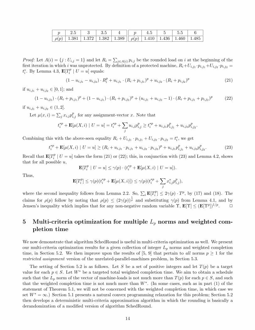
p 2.5 3 3.5 4ρ(p) 1.381 1.372 1.382 1.389

p 4.5 5 5.5 6ρ(p) 1.410 1.436 1.460 1.485

Proof: Let A(i) = {j : Ui,j = 1} and let Ri =∑

j∈A(i) pi,j be the rounded load on i at the beginning of thefirst iteration in which i was unprotected. By definition of a protected machine, Ri+Ui,j1 ·pi,j1 +Ui,j2 ·pi,j2 =t∗i . By Lemma 4.3, E[T p

i | U = u] equals:

(1− ui,j1 − ui,j2) ·Rpi + ui,j1 · (Ri + pi,j1)

p + ui,j2 · (Ri + pi,j2)p (21)

if ui,j1 + ui,j2 ∈ [0, 1]; and

(1− ui,j2) · (Ri + pi,j1)p + (1− ui,j1) · (Ri + pi,j2)

p + (ui,j1 + ui,j2 − 1) · (Ri + pi,j1 + pi,j2)p (22)

if ui,j1 + ui,j2 ∈ (1, 2].

Let µ(x, i) =∑

j xi,jppi,j for any assignment-vector x. Note that

t∗pi + E[µ(X, i) | U = u] = t∗pi +∑j

ui,jppi,j ≥ t

∗pi + ui,j1p

pi,j1

+ ui,j2ppi,j2.

Combining this with the above-seen equality Ri + Ui,j1 · pi,j1 + Ui,j2 · pi,j2 = t∗i , we get

t∗pi + E[µ(X, i) | U = u] ≥ (Ri + ui,j1 · pi,j1 + ui,j2 · pi,j2)p + ui,j1p

pi,j1

+ ui,j2ppi,j2. (23)

Recall that E[T pi | U = u] takes the form (21) or (22); this, in conjunction with (23) and Lemma 4.2, shows

that for all possible u,E[T p

i | U = u] ≤ γ(p) · (t∗pi + E[µ(X, i) | U = u]).

Thus,E[T p

i ] ≤ γ(p)(t∗pi + E[µ(X, i)]) ≤ γ(p)(t∗pi +∑j

x∗i,jppi,j),

where the second inequality follows from Lemma 2.2. So,∑

i E[T pi ] ≤ 2γ(p) · T p, by (17) and (18). The

claims for ρ(p) follow by noting that ρ(p) ≤ (2γ(p))1p and substituting γ(p) from Lemma 4.1, and by

Jensen’s inequality which implies that for any non-negative random variable Υ, E[Υ] ≤ (E[Υp])1/p. 2

5 Multi-criteria optimization for multiple Lp norms and weighted com-pletion time

We now demonstrate that algorithm SchedRound is useful in multi-criteria optimization as well. We presentour multi-criteria optimization results for a given collection of integer Lp norms and weighted completiontime, in Section 5.2. We then improve upon the results of [5, 9] that pertain to all norms p ≥ 1 for therestricted assignment version of the unrelated-parallel-machines problem, in Section 5.3.

The setting of Section 5.2 is as follows. Let S be a set of positive integers and let T (p) be a targetvalue for each p ∈ S. Let W ∗ be a targeted total weighted completion time. We aim to obtain a schedulesuch that the Lp norm of the vector of machine-loads is not much more than T (p) for each p ∈ S, and suchthat the weighted completion time is not much more than W ∗. (In some cases, such as in part (1) of thestatement of Theorem 5.1, we will not be concerned with the weighted completion time, in which case weset W ∗ =∞.) Section 5.1 presents a natural convex programming relaxation for this problem; Section 5.2then develops a deterministic multi-criteria approximation algorithm in which the rounding is basically aderandomization of a modified version of algorithm SchedRound.

14

5.1 The formulation (MULT)

Given targets {T (p) : p ∈ S} and W ∗ as in the previous paragraph, the following formulation (MULT)suggests itself. We modify the formulation of Section 4 as follows:

• we retain the constraints (15), (16) and (19);

• we include equations (17) and (18) for each p ∈ S, with the “T” in the right-hand-sides replaced by“T (p)”;

• we include constraints (8) and (9) from Section 3, with the “z” in the left-hand-sides replaced by“W ∗”;

• we replace (20) by

∀(i, j) ∈ {(i′, j′) | ∃p ∈ S such that pi′,j′ > T (p)}, xi,j = 0.

It is easy to see that the resulting formulation (MULT) is indeed a valid integer formulation of the givenproblem with targets {T (p) : p ∈ S} and W ∗. Furthermore, the discussions of Sections 3 and 4 show thatthe natural continuous relaxation of (MULT) obtained by replacing (19) by “∀(i, j), xi,j ≥ 0” is a validconvex formulation of the problem.

5.2 The rounding approach for (MULT)

Given an integer assignment X = (Xi,j), we set Cp(X) and W (X) to be the Lp norm of the vector ofmachine-loads and the weighted completion time under X, respectively. Let x∗ be a fractional assignmentthat is feasible for the continuous relaxation of (MULT). Theorem 5.1 essentially uses SchedRound to roundx∗. Note that Theorem 3.2 follows as a corollary of claim (4) of Theorem 5.1, by letting the parameter εtend to 0 from above in claim (4) of Theorem 5.1.

Theorem 5.1 Suppose, for a given problem with target machine-loads {T (p) : p ∈ S} and completion-time target W ∗, that x∗ is a feasible fractional solution to the continuous relaxation of (MULT). Then, wecan derandomize SchedRound in polynomial time to obtain an integer assignment X = (Xi,j) that achievesany desired one of the following four outcomes:

1. For all p ∈ S, Cp(X) ≤ 2.56 · T (p);

2. W (X) ≤ 3.2 ·W ∗ and for all p ∈ S, Cp(X) ≤ 3.2 · T (p);

3. For any given ε > 0, W (X) ≤ 32 · (1 + ε)W ∗ and for all p ∈ S, Cp(X) ≤ 2(e+ 2

ε ) · T (p), where e is thebase of natural logarithms; and

4. For any given ε > 0 and any given p ≥ Kε2

, W (X) ≤ 32(1 + ε) and Cp(X) ≤ 2 · T (p). (K is some

absolute constant here.)

Proof: We show how to obtain each of the four guarantees claimed in the theorem.

Guarantee 1: We now describe a derandomization of SchedRound, in order to get the guarantee for allp ∈ S. We first recall a few definitions and define new ones. Let X(h) denote the (fractional) assignmentvector after iteration h in our derandomized rounding algorithm, withX(0) .= x∗; let t∗i denote the fractionalload imposed by assignment x∗ on machine i. We let x denote an arbitrary assignment vector. For a fixed

15

machine i, let µp(x, i) =∑

j xi,jppi,j . Let X denote the final integral assignment, and let Ti denote the final

load on machine i. Let Ri, j1, and j2, denote the rounded load and the two floating jobs assigned to irespectively, at the beginning of the first iteration in which i was unprotected. Define φp(x, i) as follows:if xi,j1 + xi,j2 ∈ [0, 1], then

φp(x, i) = (1− xi,j1 − xi,j2) ·Rpi + xi,j1 · (Ri + pi,j1)

p + xi,j2 · (Ri + pi,j2)p

else if xi,j1 + xi,j2 ∈ (1, 2], then

φp(x, i) = (1− xi,j2) · (Ri + pi,j1)p + (1− xi,j1) · (Ri + pi,j2)

p + (xi,j1 + xi,j2 − 1) · (Ri + pi,j1 + pi,j2)p

This definition is motivated by the fact that φ(X, i) = T pi , just as in (21) and (22). Recall the function

γ(·) from Lemma 4.1. We next define the quantity ψp(x, i) as follows: if p = 1, then ψp(x, i) = φp(x, i);else if p > 1, then ψp(x, i) = φp(x,i)

γ(p) − t∗pi . It follows from Lemma 4.2 that for all p > 1 and ∀i, φp(x, i) ≤

γ(p)(t∗pi + µp(x, i)), and therefore we have:

ψp(x, i) ≤ µp(x, i). (24)

Let M (h)1 and M

(h)2 denote the set of protected and unprotected machines respectively immediately after

iteration h. Let Qp(X(h)) =∑

i∈M(h)1

µp(X(h), i)+∑

i∈M2ψp(X(h), i). Define Q(x) =

∑p∈S

Qp(x)f(p)·T (p)p , where

the positive values f(p) are chosen such that∑

p∈S1

f(p) ≤ 1. This implies that Q(X(0)) ≤ 1.

We are now ready to describe the derandomized version of SchedRound. At iteration h, as in therandomized version, we have two choices of assignment vectors x1 and x2 and two scalars α1, α2 ≥ 0 withα1 +α2 = 1 such that α1x1 +α2x2 = X(h). We choose X(h+1) ∈ {x1, x2} such that Q(X(h+1)) ≤ Q(X(h)).This is always possible because Q(x) is a linear function of the components in x - since we also haveQ(x) = α1Q(x1) + α2Q(x2), the minimum of these choices will not increase the value of Q. Next, if amachine i becomes unprotected during some iteration h, then for all p ∈ S, we replace µp(X(h+1), i) byψp(X(h+1), i) in the expression for Q. It follows from (24) that this replacement does not increase the valueof Q.

Since Q(X(h)) is a non-increasing function of h, Q(X) ≤ Q(X(0)) ≤ 1. Hence, it follows that for eachp ∈ S, Qp(X) ≤ f(p)T (p)p. We now analyze the final Lp norms for each p. If p = 1, the final costC1(X) =

∑i φ1(X, i) = Q1(X) ≤ f(1)T (1). We now analyze the values Cp(X) for norms p > 1. We first

note that all machines become unprotected by the time the algorithm terminates. Hence,

(Cp(X))p =∑

i

φp(X, i)

=∑

i

γ(p)(ψp(X, i) + t∗pi )

= γ(p)(∑

i

t∗pi +Qp(X))

≤ γ(p)(T (p)p + f(p)T (p)p)

≤ γ(p)(f(p) + 1)T (p)p.

Hence, Cp(X) ≤ (γ(p)(1 + f(p)))1pT (p). We are now left to show the choice of values f(p) such that

f(1) = 2.56, and for all integers p > 1, (γ(p)(1 + f(p)))1p ≤ 2.56 with

∑∞p=1

1f(p) ≤ 1. Let k = 1.28. We

choose f(p) as follows: f(1) = 2k; for p ∈ {2, 3, 4, 5, 6}, f(p) = (2k)p

γ(p) − 1; for p ≥ 7, f(p) = 4kp − 1. By

16

substituting the minimum achievable value γ(p) for each p from Lemma 4.1, we have (γ(p)(1 + f(p)))1p ≤

2.56 for every integer p. Next, observe that

∞∑p=7

1f(p)

≤∫ ∞

6

dr

4kr − 1=

1log k

· log4k6

4k6 − 1.

By substituting the value k = 1.28, it follows that∑∞

p=11

f(p) ≤ 1.

Guarantees 2, 3, and 4: We now have the problem of simultaneously minimizing the total weightedcompletion time and Lp norms for the given set of integer-norms S. We proceed quite similarly as inour approach above for Guarantee 1; we will suitably modify our “potential function” Q(·) in order toaccommodate the weighted completion-time, and employ Lemmas 2.2 and 3.1 in analyzing the effect ofthis modification.

Recall the definitions of Qp() from the proof of Guarantee 1 above. Also recall that the total weightedcompletion time objective for any integral assignment X is

W (X) =∑

i

wi,jXi,j · (pi,j +∑

j′≺ij

Xi,j′pi,j′).

We extend this definition to any fractional assignment x:

W (x) .=∑

i

wi,jxi,j · (pi,j +∑

j′≺ij

xi,j′pi,j′).

We now redefine our combined objective Q(x) as follows:

Q(x) =2W (x)3gW ∗ +

∑p∈S

Qp(x)f(p) · T (p)p

,

where the positive values g and {f(p)} satisfy

1g

+∑p∈S

1f(p)

≤ 1. (25)

We will choose these positive values separately for each of guarantees 2, 3, and 4. Recall the easy fact“W (x∗) ≤ 3W ∗/2” (e.g., from the proof of Theorem 3.2). Since X(0) = x∗, x∗ is a feasible assignment, and(25) is true, we get that Q(X(0)) ≤ 1. We now follow the same derandomization strategy as in Guarantee1: i.e., we choose from two possible choices for X(h+1) such that Q(X(h+1)) ≤ Q(X(h)). Crucially, weremark that this is possible since, as shown in Lemma 3.1, at every iteration h, the two choices for X(h+1)

namely x1 and x2, and the scalars α1, α2 ≥ 0 with α1 + α2 = 1 are such that α1 · x1 + α2 · x2 = X(h) andα1W (x1)+α2W (x2) ≤W (X(h)); this implies that at every iteration of the derandomized algorithm, thereexists a choice of X(h+1) such that Q(X(h+1)) ≤ Q(X(h)) ≤ 1. Thus we will have W (X) ≤ 3g

2 W∗ for our

final integral assignment X. We are now left to show the choice of positive values {f(p)} and g such that(25) holds, and such that the tradeoffs claimed in the theorem can be achieved. We show this below foreach of guarantees 2, 3, and 4.

Guarantee 2. We fix k = 1.6 and let g = 4k3 . All the values of f(p) remain the same function of k as in

the proof guarantee 1: i.e., f(1) = 2k, ∀p ∈ {2, . . . , 6}, f(p) = (2k)p

γ(p) − 1, and for p ≥ 7, f(p) = 4kp − 1. Itnow follows from the arguments for guarantee 1 that (25) holds.

Guarantee 3. Fix k = e + 2ε and g = 1 + ε. We let f(1) = 2k and for p ≥ 2, we let f(p) = 4kp − 1

and γ(p) = 2p−2 (from Lemma 4.2). This yields an approximation factor of 3(1+ε)2 for the completion

17

time and a factor of 2(e + 2ε ) for each norm p ∈ S. We now have, 1

g +∑

p∈S1

f(p) ≤1

1+ε +∑∞

p=11

f(p) ≤1− ε

2 + ε4 + 1

log k · log( 4k4k−1) ≤ 1− ε

2 + ε4 + 1

4k−1 ≤ 1− ε2 + ε

4 + ε8 ≤ 1.

Guarantee 4. Fix g = (1 + ε), and let f(p) = 1 + 1ε . We have γ(p) ≤ O( 2p

√p) from Lemma 4.2. Hence

for all p ≥ K/ε2 with K being a suitably large constant, γ(p) ≤ ε2p−2. So, W (X) ≤ 3(1+ε)2 · W ∗ and

Cp(X) ≤ (γ(p)(f(p) + 1))1pT (p) ≤ 2T (p). Furthermore, 1

g + 1f(p) = 1, which concludes the proof of the

theorem. 2

5.3 All-norm approximations for the restricted assignment problem

The next theorem pertains to the approximation ratio of SchedRound for the restricted assignment problem,where each job j is associated with some number pj such that for all (i, j), pi,j ∈ {pj ,∞}. That is, eachjob has a processing time pj and a subset Sj of the machines; j can only be scheduled on some machine inSj , and has processing time pj on all machines in Sj . We will employ Theorem 4.4 to improve on certainresults of [5, 9].

As in Azar et al. [5], we first obtain the unique fractional solution x∗ that is simultaneously optimalwith respect to all norms p ≥ 1: this x∗ is a strongly-optimal fractional assignment, in the following sense[5]. Consider a fractional assignment x′; let t′i be the fractional load on machine i induced by x′: i.e.,t′i =

∑j∈J x

′i,jpi,j . Consider any norm p ≥ 1; the fractional Lp-norm of x′ is Lp(x′) = (

∑i∈M (t′i)

p)1p ; let

Lp(frac) denote the minimum value of the Lp-norm achievable by any valid fractional assignment (i.e., anyfractional assignment such that the xi,j are all non-negative, and such that the sum of the xi,j values for eachjob j is one); let Lp(int) denote the minimum value of Lp-norm achievable by any valid integral assignment.A fractional assignment x∗ is strongly-optimal if for any p ≥ 1, Lp(x∗) = Lp(frac) (i.e, x∗ is optimal w.r.t.all the norms). Azar et al. [5] show that, given any instance of the restricted assignment problem, thereexists a strongly-optimal fractional assignment x∗ for the instance; further, such an assignment can becomputed in polynomial time. It is also demonstrated in [5] that x∗ can be rounded efficiently to get anabsolute 2-approximation factor w.r.t. every norm p ≥ 1: this notion of absolute approximation is thateach Lp norm is individually at most twice optimal, i.e., at most 2 · Lp(int). This result of [5] was alsoindependently shown by Goel and Meyerson [9]. We get an improvement as follows:

Theorem 5.2 Consider the restricted assignment problem. Given a strongly-optimal fractional assignmentx∗, and a fixed norm p′ ∈ [1,∞), SchedRound can be derandomized in polynomial time to simultaneouslyyield a ρ(p′) < 2 absolute approximation w.r.t. norm p′ and an absolute 2-approximation w.r.t. all othernorms p ≥ 1, where ρ(·) is the function from Theorem 4.4. That is, the Lp norms Cp of the integralsolution constructed, satisfy the following: Cp ≤ 2 · Lp(int) for all p ≥ 1, and Cp′ ≤ ρ(p′) · Lp′(int).

Proof: We start by computing a strongly-optimal fractional assignment x∗ as in Azar et al. [5]. We roundthis fractional assignment into an integral assignment using algorithm SchedRound. Let Cp be the randomvariable denoting the Lp norm of the integral assignment produced by our algorithm. We prove below thatfor all p ≥ 1, Cp ≤ 2Lp(int) with probability 1. This claim along with Theorem 4.4 immediately leads toTheorem 5.2 as follows. Consider the fixed norm p′ ∈ [1,∞); the fractional assignment has an Lp′ normvalue of Lp′(x∗) = Lp′(frac) ≤ Lp′(int). Hence, by Theorem 4.4, the integral assignment has an expectedvalue E[Cp′ ] such that E[Cp′ ] ≤ ρ(p′)Lp′(frac) ≤ ρ(p′)Lp′(int); here ρ(p′) < 2 is the approximation ratioin Theorem 4.4. Crucially, since our claim guarantees that ∀p ≥ 1, Cp ≤ 2Lp(int) with probability 1, wehave the conditional expectation E[Cp′ | ∀p ≥ 1, Cp ≤ 2Lp(int)] = E[Cp′ ] ≤ ρ(p′)Lp′(int). Hence, we canderandomize algorithm SchedRound using the method of conditional probabilities (as in Theorem 4.4) toobtain an integral assignment such that Cp′ ≤ ρ(p′)Lp′(int) and ∀p ≥ 1, Cp ≤ 2Lp(int).

18

We now prove that SchedRound produces an integral assignment in which for all p ≥ 1, Cp ≤ 2Lp(int)with probability 1. Let X = (Xi,j) denote the integral assignment yielded by SchedRound; recall thatSchedRound ensures that Xi,j can be 1 only if x∗i,j > 0. Since we have an instance of restricted assignmentand x∗ is an optimal fractional assignment w.r.t. all the norms, it follows that Xi,j = 1 only if pi,j = pj

(and not ∞). We have

(Cp)p =∑

i

(∑j∈J

Xi,j · pi,j)p

<∑

i

(∑j∈J

x∗i,j · pi,j) + maxj∈J : Xi,j=1

pi,j

p

(26)

≤∑

i

2p−1 ·

(∑j∈J

x∗i,j · pi,j)p + ( maxj∈J : Xi,j=1

pj)p

(27)

≤ 2p−1 ·

(∑

i

(∑j∈J

x∗i,j · pi,j)p) +∑j

ppj

≤ 2p−1 · (Lp(frac)p + Lp(int)p) (28)

≤ 2p−1 · 2Lp(int)p

= 2p · Lp(int)p

Hence: Cp ≤ 2Lp(int)

In the above derivation, (26) follows from Lemma 2.3(ii). Bound (27) is a consequence of the fact that forall x ≥ 0, y ≥ 0 and p ≥ 1, (x+ y)p ≤ 2p−1 · (xp + yp). Bound (28) follows from the fact that (

∑j p

pj )

1p is

a lower bound on the Lp norm value of any integral assignment. 2

6 Generalizing the Karp et al. Procedure, and Applications

We now employ LinAlgRound to develop two additional applications. The 2-approximation for makespanminimization in unrelated parallel machines [18] was extended in [21] as follows. Suppose we are givensome numbers {ci,j} (where ci,j corresponds, e.g., to the cost of processing job j on machine i), a targetmakespan T , and a fractional assignment x that satisfies the target makespan (along with the usualimportant constraints “if pi,j > T , then xi,j = 0”) as well as the constraint

∑i,j ci,jxi,j = C for some

C. Then, the algorithm of [21] constructs an integral assignment X such that∑

j pi,jXi,j ≤ 2T for alli, and such that

∑i,j ci,jXi,j ≤ C. We first describe how Theorem 6.1, a basic rounding theorem of

Karp et al. [13], can be used to obtain the result of [18]. We then show a probabilistic generalization ofthis theorem of [13] (Theorem 6.2) which in particular also yields the result of [21]. We also describe anextension (Corollary 6.4) to the setting where we are given multiple cost-objectives and by paying a slightlylarger factor for the makespan, we can bound the absolute deviation for the additional objectives.

Theorem 6.1 ([13]) Given a matrix A ∈ <m×n, with t denoting maxj{∑

i:Aij>0Aij ,−∑

i:Aij<0Aij}, anda fractional vector x, we can, in deterministic polynomial time, construct a vector X such that: (i) ∀j,Xj ∈ {bxjc, dxje}, and (ii) ∀i, (AX)i < (Ax)i + t.

To see how Theorem 6.1 yields the result of [18], consider the LP of [18] for makespan minimization,given a target makespan of T :

19

(A1) ∀j,∑

i xi,j ≥ 1;

(A2) ∀i,∑

j pi,jxi,j ≤ T ;

(A3) 0 ≤ xi,j ≤ 1; and

(A4) pi,j > T implies xi,j = 0.

If we multiply the constraints (A1) by −T , the parameter t, in the notation of Theorem 6.1, can be takento be T ; therefore there is an integral vector X such that: (i) for each j,

∑i−Xi,j < 0, or

∑iXi,j ≥ 1 (i.e.,

job j is assigned to some machine), and (ii) for each i,∑

j pi,jXi,j ≤ 2T . We now describe our probabilisticgeneralization of Theorem 6.1; it is a generalization since it guarantees the additional properties (iii) and(iv):

Theorem 6.2 Given a matrix A ∈ <m×n, with t denoting maxj{∑

i:Aij>0Aij ,−∑

i:Aij<0Aij}, and ann-dimensional vector x, we can, in randomized polynomial time, construct a vector X such that: (i) ∀j,Xj ∈ {bxjc, dxje} with probability 1, (ii) ∀i, (AX)i < (Ax)i + t with probability 1, and (iii) for each j,E[Xj ] = xj; in particular, given any vector ~c, we have E[

∑j cjXj ] = C

.=∑

j cjxj. Furthermore: (iv)a vector X for which (i) and (ii) hold, and for which

∑j cjXj ≤ C, can be constructed in deterministic

polynomial time.

Proof: We essentially use algorithm LinAlgRand on top of the basic approach of Theorem 6.1 as follows.By subtracting out integer parts, we may assume that xj ∈ [0, 1] for all j. We proceed in iterations, eachof which further rounds at least one yet-unrounded xj to 0 or 1. We now describe a typical iteration.Suppose L is the current linear system (when we start, L is the original system “Ax = b”). Recall theSimplify operation related to LinAlgRand. We first run Simplify to make L canonical. Now, it is shownin [13] that: (a) either L is under-determined, or (b) there exists a row i (which can be found efficiently)in our system of constraints L such that no matter how we round the yet-unrounded variables to geta final (rounded) vector X, we will have (AX)i < bi + t. If (b) holds, we keep discarding such rows ifrom consideration (since they are “safe” from now on), until case (a) holds. And now that the system isunder-determined, we apply RandStep. This completes the description of an iteration.

Lemma 2.4 easily shows properties (i), (ii) and (iii) of the theorem. Property (iv) also follows directlyby derandomizing this algorithm – i.e., making each application of RandStep deterministic – using themethod of conditional probabilities as follows. Suppose S is the current set of yet-unrounded variables,and that RandStep has the choice of moving along directions ~r or −~r: then, we choose ~r if

∑j∈S cjrj ≤ 0,

and choose −~r otherwise. 2

Recall the argument above (using the constraints (A1)–(A4)), about how Theorem 6.1 yields theresult of [18]; Theorem 6.2 can be similarly seen to imply the result of [21].

We now extend Theorem 6.2 as follows. Suppose, in addition to the linear system Ax = b, we have`+ 1 additional linear constraints c(k) · x = dk, k = 0, 1, . . . `. We prove that these additional constraintscan be approximated well, by incurring a slightly larger error in the system “Ax = b”:

Corollary 6.3 Suppose we are given: (i) a matrix A ∈ <m×n, with the parameter t as in Theorem 6.2;(ii) an n-dimensional vector x, (iii) ` + 1 linear constraints c(k) · x = dk, k = 0, 1, . . . `, that are satisfiedby the given x, and (iv) a positive real ε. We can, in deterministic polynomial time, construct a vector Xsuch that:

(a) ∀j, Xj ∈ {bxjc, dxje};

20

(b) ∀i, (AX)i < (Ax)i + t(1 + ε);

(c) for all k = 1, 2, . . . , `, |c(k) ·X − dk| ≤ (1 + ε)Mk`/ε, where Mk is the maximum absolute value of anycoefficient in c(k) (note that the case k = 0 is excluded here, and is handled next in part (d)); and

(d) c(0) ·X ≤ d0.

Proof: We will first rescale the given system with constraints “Ax = b” and “c(k) · x = dk, k = 1, . . . `”(note that the constraint for k = 0 is excluded here) as follows: scale the system “Ax = b” by 1/((1 + ε)t),and replace the constraints “c(k) · x = dk, k = 1, . . . `” by the following 2` constraints:

ε

(1 + ε) · ` ·Mk· (c(k) · x) ≤ ε

(1 + ε) · ` ·Mk· dk; k = 1, . . . `;

− ε

(1 + ε) · ` ·Mk· (c(k) · x) ≤ − ε

(1 + ε) · ` ·Mk· dk; k = 1, . . . `.

Note that the parameter t for this system, in the notation of Theorem 6.2, is at most

t

(1 + ε)t+

∑̀k=1

εMk

(1 + ε) · ` ·Mk= 1,

where the “Mk” in the numerator of the second term in the l.h.s. comes from the fact that Mk is themaximum absolute value of any coefficient in c(k). Now apply part (iv) of Theorem 6.2, with the constraint“c(0) · x = d0” playing the role of the constraint “

∑j cjxj = C” of Theorem 6.2. We now verify that the

resultant vector X satisfies the guarantees of this corollary. Guarantees (a) and (d) directly follow fromTheorem 6.2. Guarantee (b) follows from Theorem 6.2, via a rescaling by (1 + ε)t. Similarly, Guarantee(c) follows from rescaling by the quantities (1+ε)·`·Mk

ε . 2

Using the constraints (A1)–(A4) once again, Corollary 6.3 specializes to the following result on multi-objective scheduling:

Corollary 6.4 Suppose we are given an instance of unrelated-machine-scheduling the cost of processingjob j on machine i), a target makespan T , and a fractional assignment x that satisfies the target makespan,as well as the constraints “if pi,j > T , then xi,j = 0”. Suppose further that x satisfies the ` + 1 linearconstraints c(k) · x = dk, k = 0, 1, . . . `. Then, for any given ε > 0, we can construct an integral scheduleX = (Xi,j) such that:

(a) the makespan is at most (2 + ε)T ;

(b) for all k = 1, 2, . . . , `, |c(k) ·X − dk| ≤ (1 + ε)Mk`/ε, where Mk is the maximum absolute value of anycoefficient in c(k); and

(c) c(0) ·X ≤ d0.

Note in particular that for bounded Mk, ` and ε, we get a constant additive error for the additionalconstraints; we are not aware of any other method that can yield this, even for small constants `.

Finally, we consider the problem of unrelated parallel machine scheduling with resource dependentprocessing times. This is a variant of the standard unrelated parallel machine scheduling, where theprocessing times pi,j of any machine-job pair can be reduced by utilizing a renewable resource (such asadditional workers) that can be distributed over the jobs. Specifically, a maximum number of k units ofa resource may be used to speed up the jobs, and the available amount of k units of that resource must

21

not be exceeded at any time. Grigoriev et al. [11] presented a 4 + 2√

2 approximation for this problem. Adirect application of Theorem 6.2 yields an assignment of jobs and resources to machines; combined withthe scheduling algorithm of [11], we developed in the conference version of this work [15] a 4-approximationfor the problem. Our work has been further built upon in [12], leading to a 3.75-approximation. We referthe reader to [12] for complete details, but the basic idea for our improvement exactly follows from the factthat Theorem 6.2 is able to incorporate one additional linear constraint (i.e., via ~c), without losing any ofthe guarantees of Theorem 6.1.

7 Convergence to fairness

Quite a number of our bounds are of the following type. Some random variable X:

(P1) has “low” expectation µ (often equal to the corresponding LP-value), and

(P2) is at most some value a with probability 1.

Two examples of this are as follows: (a) as seen from Sections 2 and 3, SchedRound ensures that the finalload on machine i,

∑j pi,jXi,j , equals its LP-value t∗i in expectation, and is at most 2t∗i with probability

one; (b) properties (ii) and (iii) of Theorem 6.2 show that for any row i, (AX)i equals (Ax)i in expectation,and is less than (Ax)i + t with probability one. We often use only (P2) in bounding our approximationguarantees; in this short section, we observe that combined usage of (P1) and (P2) easily leads to fairnessguarantees under multiple executions.

Consider, for instance, the makespan-minimization setting described in application (iv) in the introduc-tion; the reader is asked to recall the notation used therein. From the discussion of the previous paragraph,we have that for any i and k, Zi,k lies in [0, 2], and has mean at most 1. Thus, since Zi,k is a boundedrandom variable, a standard application of the Chernoff bounds shows that for any particular i,

Pr[Zi(N) > (1 + ε)]� 1/m,

if N ≥ K(logm)/ε2. Thus, a union bound over all m indices i gives simultaneous fairness for all machines,with high probability. Similar fairness considerations apply to any random variable of the type consideredin the previous paragraph.

8 Conclusions

We have presented a new approach to scheduling through SchedRound, which is a rounding algorithmbased on linear algebra and randomization. SchedRound offers a unified way to tackle a number of differentobjectives in scheduling jobs on unrelated parallel machines. One natural question left open is to improvethe specific bounds developed in this paper: e.g., can we do better for at least one of the pair (makespan,weighted completion time) of objectives? Also, could linear-algebraic considerations help with roundingfor semidefinite programs, where variants of the seminal random-hyperplane technique [10] appear to bethe foremost tools of choice?

As mentioned in Section 6, our work has been used to develop improved approximation algorithms forscheduling problems where processing times are a function of the number of resources deployed [12]. Ourmethods have also been put to use in [16] for game-theoretic issues in scheduling. We anticipate furthersuch applications in the field of approximation algorithms.

22

Acknowledgments. We thank David Shmoys for valuable discussions, Cliff Stein for introducing usto [24], and Yossi Azar for sending us an early version of [4]. We are thankful to the FOCS 2005 andJACM referees for their valuable comments. V. S. A. Kumar and M. V. Marathe thank their externalcollaborators and members of the Network Dynamics and Simulation Science Laboratory (NDSSL) fortheir suggestions and comments. This research of Kumar and Marathe has been partially supported byNSF NeTS Grant CNS-0626964, NSF HSD Grant SES-0729441, CDC Center of Excellence in Public HealthInformatics Grant 2506055-01, NIH-NIGMS MIDAS Project 5 U01 GM070694-05, DTRA CNIMS GrantHDTRA1-07-C-0113 and NSF NeTS Grant CNS-0831633. S. Parthasarathy’s research has been supportedin part by NSF Award CCR-0208005 and NSF ITR Award CNS-0426683. A. Srinivasan’s research hasbeen supported in part by NSF Award CCR-0208005, NSF ITR Award CNS-0426683, and NSF AwardCNS-0626636.

References

[1] Alon, N., Azar, Y., Woeginger, G. J., and Yadid, T. Approximation schemes for scheduling.In Proc. ACM-SIAM Symposium on Discrete Algorithms (1997), pp. 493–500.

[2] Aslam, J., Rasala, A., Stein, C., and Young, N. Improved bicriteria existence theorems forscheduling. In Proc. ACM-SIAM Symposium on Discrete Algorithms (1999), pp. 846–847.

[3] Awerbuch, B., Azar, Y., Grove, E. F., Kao, M.-Y., Krishnan, P., and Vitter, J. S. Loadbalancing in the Lp norm. In Proc. IEEE Symposium on Foundations of Computer Science (1995),pp. 383–391.

[4] Azar, Y., and Epstein, A. Convex programming for scheduling unrelated parallel machines. InProc. of the ACM Symposium on Theory of Computing (2005), pp. 331–337.

[5] Azar, Y., Epstein, L., Richter, Y., and Woeginger, G. J. All-norm approximation algorithms.J. Algorithms 52, 2 (2004), 120–133.

[6] Azar, Y., and Taub, S. All-norm approximation for scheduling on identical machines. In Proc.Scandinavian Workshop on Algorithm Theory (2004), pp. 298–310.

[7] Chandra, A. K., and Wong, C. K. Worst-case analysis of a placement algorithm related to storageallocation. SIAM J. on Computing 4, 3 (1975), 249–263.

[8] Gandhi, R., Khuller, S., Parthasarathy, S., and Srinivasan, A. Dependent rounding andits applications to approximation algorithms. Journal of the ACM 53 (2006), 324–360.

[9] Goel, A., and Meyerson, A. Simultaneous optimization via approximate majorization for concaveprofits or convex costs. Tech. Report CMU-CS-02-203, December 2002, Carnegie-Mellon University.

[10] Goemans, M. X., and Williamson, D. P. Improved approximation algorithms for MaximumCut and Satisfiability problems using Semidefinite Programming. Journal of the ACM 42 (1995),1115–1145.

[11] Grigoriev, A., Sviridenko, M., and Uetz, M. Unrelated parallel machine scheduling withresource dependent processing times. In Proc. Integer Programming and Combinatorial Optimization(IPCO) (2005), pp. 182–195.

[12] Grigoriev, A., Sviridenko, M., and Uetz, M. Machine scheduling with resource dependentprocessing times. Mathematical Programming 110 (2007), 209–228.

23

[13] Karp, R. M., Leighton, F. T., Rivest, R. L., Thompson, C. D., Vazirani, U. V., andVazirani, V. V. Global wire routing in two-dimensional arrays. Algorithmica (1987), 113–129.

[14] Kleinberg, J., Tardos, E., and Rabani, Y. Fairness in routing and load balancing. J. Comput.Syst. Sci. 63, 1 (2001), 2–20.

[15] Kumar, V. S. A., Marathe, M. V., Parthasarathy, S., and Srinivasan, A. Approxima-tion algorithms for scheduling on multiple machines. In Proc. IEEE Symposium on Foundations ofComputer Science (2005), pp. 254–263.

[16] Lavi, R., and Swamy, C. Truthful mechanism design for multi-dimensional scheduling via cyclemonotonicity. In Proc. ACM Conference on Electronic Commerce (2007), pp. 252–261.

[17] Lawler, E. L., Lenstra, J. K., Kan, A. H. G. R., and Shmoys, D. B. Sequencing andscheduling: algorithms and complexity. Elsevier, 1993.

[18] Lenstra, J. K., Shmoys, D. B., and Tardos, E. Approximation algorithms for schedulingunrelated parallel machines. Mathematical Programming (1990), 259–271.

[19] Raghavan, P., and Thompson, C. D. Randomized rounding: a technique for provably goodalgorithms and algorithmic proofs. Combinatorica (1987), 365–374.

[20] Schuurman, P., and Woeginger, G. J. Polynomial time approximation algorithms for machinescheduling: Ten open problems. J. Scheduling (1999), 203–213.

[21] Shmoys, D. B., and Tardos, E. An approximation algorithm for the generalized assignmentproblem. Mathematical Programming (1993), 461–474.

[22] Skutella, M. Convex quadratic and semidefinite relaxations in scheduling. Journal of the ACM 46,2 (2001), 206–242.

[23] Smith, W. E. Various optimizers for single-stage production. Nav. Res. Log. Q. (1956), 59–66.

[24] Stein, C., and Wein, J. On the existence of schedules that are near-optimal for both makespanand total weighted completion time. Operations Research Letters 21 (1997), 115–122.

Appendix

A Proofs and Auxiliary Results

Proof: (For Lemma 4.1) Consider any p ≥ 1. Let N ′(a, λ) = pa · (1 + λ)p−1 and D′(a, λ) = pa ·(1 + aλ)p−1 + paλp−1 be the derivatives of N(a, λ) and D(a, λ) respectively w.r.t. λ. Observe thatN(a, λ) = N(a, 0) +

∫ λ0 N

′(a, λ)dλ and DN(a, λ) = D(a, 0) +∫ λ0 D

′(a, λ)dλ. Hence,

maxa,λ

N(a, λ)D(a, λ)

≤ max{N(a, 0)D(a, 0)

,maxa,λ

N ′(a, λ)D′(a, λ)

}.

We have maxa,λN ′(a,λ)D′(a,λ) ≤

(1+λ)p−1

1+λp−1 which is maximized when λ = 1. Hence maxa,λN(a,λ)D(a,λ) ≤ max{1, 2p−2}.

Thus the lemma holds for the first two cases.

Now suppose p is sufficiently large. Observe that

N(a, λ)D(a, λ)

≤ Λ .=a(1 + λ)p + 1− a

1 + paλ+ aλp.

24

We now analyze Λ. Both the numerator and denominator of Λ are linear functions of a, and the denominatoris positive; so, Λ is maximized when a ∈ {0, 1}. When a = 0, Λ = 1 and the lemma holds. Hence, it isenough to show that F (λ) .= (1+λ)p

1+pλ+λp is at most O(2p/√p). If λ ≤ 1

2 , then F (λ) ≤(

32

)p; else if λ ∈ [12 , 1],

the denominator of F (λ) is at least p2 and the numerator is at most 2p. Hence the lemma holds if λ ∈ [0, 1].

Assume next that λ > 1, and set λ = 1+ε1−ε for some positive ε. Then,

F (λ) ≤ 2p

p(1− ε)p + (1 + ε)p. (29)

The denominator here is minimized when

1 + ε

1− ε= p

1p−1 = e(ln p)/(p−1) = 1 +

ln pp±O((

ln pp

)2).

We thus take ε = ln p2p ±O(( ln p

p )2). This implies that 1+ε = 1+ ln p2p ±O(( ln p

p )2) and 1−ε = 1− ln p2p ±O(( ln p

p )2).Substituting back these values in (29) yields

F (λ) ≤ 2p

p · [1− (ln p)/(2p)±O(((ln p)/p)2)]p + [1 + (ln p)/(2p)±O(((ln p)/p)2)]p

= Θ(2p/(p · 1/√p+√p))

= Θ(2p/√p).

Thus we have the lemma’s claim for large p.

Finally, suppose p ∈ S = {2.5, 3, 3.5, 4, 4.5, 5, 5.5, 6}. We use numerical techniques to obtain tighterbounds on γ(p). Define f(a, λ) .= (1 + aλ)p and g(a, λ) .= 1

γ(p) + a · (1+λ)p−1−γ(p)λp

γ(p) . For each p ∈ S, itsuffices to show for all (a, λ) ∈ [0, 1]× [0,∞) that

f(a, λ) ≥ g(a, λ). (30)

For any fixed λ, f(a, λ) is a convex function of a while g(a, λ) is linear. Assume γ(p) > 1. Hence,f(0, λ) ≥ g(0, λ) and f(1, λ) ≥ g(1, λ). Hence, if (30) is violated, then the straight line g(a, λ) intersectsthe convex function f(a, λ) at two distinct values of a ∈ (0, 1). In this case, by Lagrange’s Mean ValueTheorem, there exists an a ∈ (0, 1) such that f ′(a, λ) (derivative w.r.t. a), i.e., pλ(1 + aλ)p−1, equals(1+λ)p−1−γ(p)λp

γ(p) . Let a∗(λ) be this value which can be obtained by solving this equation for a. Since f isstrictly convex as a function of a, f(a∗(λ), λ) < g(a∗(λ), λ). The above arguments yield us the followingstrategy for choosing γ(p). We choose γ(p) such that one of the following conditions hold for λ ∈ [0, 15].

1. a∗(λ) < 0. In this case both the intersection points of g(a, λ) and f(a, λ) are at values a ≤ 0. Hence,g(a, λ) ≤ f(a, λ) for all values of a ∈ [0, 1] and our claims hold.

2. f(a∗(λ), λ) − g(a∗(λ), λ) ≥ 0. In this case the functions do not intersect within the ranges of a andλ that are of interest to us.

For the choices of γ(p) in this lemma, one of these two conditions occurs and this can be verified numericallyby plotting the above functions of λ in the range λ ∈ [0, 15]. We restrict ourselves to λ ∈ [0, 15] since thefraction N(a,λ)

D(a,λ) for the values of λ > 15 can be easily seen to be within γ(p) for the values of p consideredhere. This completes the proof of the lemma. 2

Proof: (For Lemma 4.2) Recall that p, λ1, λ2 are arbitrary but fixed positive values with p > 1; also,λ0 is some non-negative constant. In all the cases below, we assume w.l.o.g. that λ1 ≥ λ2. Let us first

25

dispose of the easy case where λ0 = λ2 = 0. In this case, N = a1λp1 regardless of the value of a1 + a2, and

D = (ap1 + a1) · λp; so, N ≤ D. Note from Lemma 4.1 that γ(p) ≥ 1, since we can always set a = λ = 0 in

Lemma 4.1. So, N ≤ γ(p) ·D if λ0 = λ2 = 0.

Hence, we assume from now on that λ0 + λ2 > 0. We analyze three possible cases next.

Case 1: a1 + a2 = 1. Since a1 + a2 = 1, λ1 ≥ λ2 and λ0 + λ2 > 0, D is nonzero. We have

N

D=

a1(λ0 + λ1)p + (1− a1)(λ0 + λ2)p

(λ0 + λ2 + a1(λ1 − λ2))p + a1λp1 + (1− a1)λ

p2

≤ a1(λ0 + λ2 + (λ1 − λ2))p + (1− a1)(λ0 + λ2)p

(λ0 + λ2 + a1(λ1 − λ2))p + a1(λ1 − λ2)p

By scaling both the numerator and denominator of the latter fraction by (λ0 + λ2)p > 0, and by lettingλ = (λ1−λ2)/(λ0 +λ2) (which is non-negative since λ1 ≥ λ2 by assumption), the fraction is seen to assumethe form as in Lemma 4.1. Hence the lemma holds.

Case 2: a1 + a2 ≥ 1. In this case, D is nonzero and

N

D=

(a1 + a2 − 1)(λ0 + λ2 + λ1)p + (1− a1)(λ0 + λ2)p + (1− a2)(λ0 + λ1)p

(λ0 + a1λ1 + a2λ2)p + a1λp1 + a2λ

p2

. (31)

Let λ0 + a1λ1 + a2λ2 = φ, and hold φ fixed. Thus, we view a1 and a2 as variables subject to the followingfour linear constraints: (i) 0 ≤ a1 ≤ 1, (ii) 0 ≤ a2 ≤ 1, (iii) a1+a2 ≥ 1, and (iv) λ0+a1λ1+a2λ2 = φ, whereφ is fixed. Now, the fraction in (31) becomes a rational function of a1 and a2 with a positive denominator;so, it is maximized when (at least) two of the constraints (i)-(iv) are met with equality. If a1 +a2 = 1, thenCase 1 occurs and the lemma holds. Otherwise, either a1 or a2 is equal to 1, and a1 + a2 > 1. Supposea2 = 1 and a1 > 0. We have

N

D=

a1(λ0 + λ2 + λ1)p + (1− a1)(λ0 + λ2)p

(λ0 + λ2 + a1λ1)p + a1λp1 + λp

2

≤ a1(λ0 + λ2 + λ1)p + (1− a1)(λ0 + λ2)p

(λ0 + λ2 + a1λ1)p + a1λp1

.

If we scale both the numerator and denominator of the latter fraction by (λ0 + λ2)p > 0, it assumes thesame form as in Lemma 4.1. Hence the lemma holds. An identical argument applies when a1 = 1.

Case 3: a1 + a2 ≤ 1. If λ0 = 0, then N ≤ D and again, we get N ≤ γ(p) · D. So, we assume thatλ0 > 0, which implies that D > 0. We proceed as in Case 2, holding φ fixed; the only change is thatconstraint (iii) of Case 2 now becomes “a1 + a2 ≤ 1”. Once again, N/D is maximized when at least twoof the four constraints (i)-(iv) are met with equality, and we are reduced to Case 1 if a1 + a2 = 1. So, theonly remaining case is where one among a1 and a2 is zero, and the other is strictly smaller than 1. So,suppose a2 = 0 and 0 ≤ a1 < 1. We get

N

D=a1(λ0 + λ1)p + (1− a1)λ

p0

(λ0 + a1λ1)p + a1λp1

,

which assumes the same form as in Lemma 4.1 upon scaling the numerator and denominator by λp0. An

identical argument applies when a1 = 0. 2

26