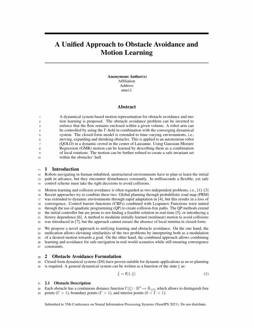
A Unified Approach to Obstacle Avoidance andMotion Learning

Anonymous Author(s)AffiliationAddressemail

Abstract

A dynamical system based motion representation for obstacle avoidance and mo-1

tion learning is proposed. The obstacle avoidance problem can be inverted to2

enforce that the flow remains enclosed within a given volume. A robot arm can3

be controlled by using the Γ-field in combination with the converging dynamical4

system. The closed-form model is extended to time-varying environments, i.e.,5

moving, expanding and shrinking obstacles. This is applied to an autonomous robot6

(QOLO) in a dynamic crowd in the center of Lausanne. Using Gaussian Mixture7

Regression (GMR) motion can be learned by describing them as a combination8

of local rotations. The motion can be further refined to create a safe invariant set9

within the obstacles’ hull.10

1 Introduction11

Robots navigating in human-inhabited, unstructured environments have to plan or learn the initial12

path in advance, but they encounter disturbances constantly. In milliseconds a flexible, yet safe13

control scheme must take the right decisions to avoid collisions.14

Motion learning and collision avoidance is often regarded as two independent problems, i.e., [1]–[3]15

Recent approaches try to combine these two. Global planning through probabilistic road map (PRM)16

was extended to dynamic environments through rapid adaptation in [4], but this results in a loss of17

convergence. Control barrier functions (CBFs) combined with Lyapunov Functions were united18

through the use of quadratic programming (QP) to create collision-free paths. The QP methods extend19

the initial controller but are prone to not finding a feasible solution in real-time [5], or introducing a20

history dependence [6]. A method to modulate initially learned (nonlinear) motion to avoid collisions21

was introduced in [7], but the approach cannot ensure the absence of local minima in closed-form.22

We propose a novel approach to unifying learning and obstacle avoidance. On the one hand, the23

unification allows elevating similarities of the two problems by interpreting both as a modulation24

of a desired motion towards a goal. On the other hand, the combined approach allows combining25

learning and avoidance for safe navigation in real-world scenarios while still ensuring convergence26

constraints.27

2 Obstacle Avoidance Formulation28

Closed-form dynamical systems (DS) have proven suitable for dynamic applications as no re-planning29

is required. A general dynamical system can be written as a function of the state ξ as:30

ξ̇ = f(t, ξ) (1)

2.1 Obstacle Description31

Each obstacle has a continuous distance function Γ(ξ) : Rd 7→ R≥0, which allows to distinguish free32

points (Γ > 1), boundary points (Γ = 1), and interior points (0 < Γ < 1).33

Submitted to 35th Conference on Neural Information Processing Systems (NeurIPS 2021). Do not distribute.

Additionally a reference point ξri is chosen within its boundaries. This allows to define the reference34

direction towards the obstacle as ro(ξ) = (ξ − ξri )/‖ξ − ξri ‖.35

2.2 Obstacle Avoidance through Modulation36

In [8], real-time obstacle avoidance is obtained by applying a dynamic modulation matrix to a37

dynamical system f(ξ):38

ξ̇ = M(ξ)f(ξ) with f(ξ) = k(ξ − ξa) (2)

Describing the obstacle avoidance as a modulation of the initial dynamics ensured that attractors are39

conserved, i.e. 0 = M(ξ)0. Additionally, no spurious (new) attractors are introduced, as long as the40

matrix M(ξ) has full rank.41

We will focus on motion with a clearly defined goal (i.e. attractor ξa). The scaling parameter k42

introduces change with respect to time. It is of unit s−1.43

44

2.2.1 Fluid Dynamic Inspired Compression and Stretching45

The potential (laminar) flow of an incompressible fluid around a cylinder is a known problem46

in fluid dynamics with known closed-form description It will serve as a basis for the obstacle47

avoidance algorithm. Similarly to the potential flow, the vector field is scaled in tangent and radial48

direction. Hence, the modulation matrix is defined as M(ξ) = E(ξ)D(ξ)E(ξ)−1, a function of the49

decomposition matrix E(ξ) and the diagonal scaling matrix D(ξ).50

2.2.2 Modulation through Decoupling of Rotation and Stretching51

Alternatively, any vector transformation can be interpreted as a rotation with matrix R(ξ) and a52

stretching h(x). This concept has been used in two dimensions for local modulation by [9]:53

ξ̇ = h(ξ)R(ξ) f(ξ) (3)

The rotation can alternatively be applied by using the orientation-space transform described in [10]54

(instead of the matrix modulation by R(ξ)).55

2.3 Multiple Obstacles56

In the presence of multiple obstacles, the velocity is modulated for each obstacle individually. The57

final velocity is obtained by taking the weighted mean in direction space in [8]. This has been applied58

in Fig. 1.59

f(ξ)ξ

r(ξ)e(ξ)

Γ(ξ)=1

fr(ξ)

fe(ξ)ξa ξr

Γ(ξ)=2 Γ(ξ)=3

(a) Γ-function

f(ξ)

ξ ξ

ξrξa

ξeξr

(b) Avoidance of circle (c) Non-smooth edges (d) Multiple obstacles

Figure 1: Obstacle avoidance around a single and multiple obstacles.

3 Inverted Obstacle Avoidance60

An autonomous robot might be in a scenario where it has boundaries which cannot be pass. This61

might be a wall for a wheeled robot, or it can be safety or joint limits for a robot arm. This is stated as62

the constraint of staying within an obstacle, where the boundary of the obstacle represents the limits63

of the free space.64

3.1 Distance Inversion65

If we use the previously introduced obstacle description to denote enclosing hulls, the interior points66

of the classical obstacle become points of free space of the enclosing hull and vice versa. For this67

reason, we introduce the inverted distance function Γw as:68

Γw(ξ) = 1/Γo = (R(ξ)/‖ξ − ξr‖)2p ∀ Rd \ ξr (4)

2

This allows to treat boundaries the previously defined algorithm (but the newly introduced Γw). It69

follows that convergence is still ensured.70

3.2 Gaps in the Wall71

In many practical scenarios a hull entails gaps or holes through which the agent enters or exits the72

space (e.g., door in a room). The inverted obstacle avoidance slows the agent down to zero while it73

is trying to approach this exit. For this reason, a guiding reference point for boundary obstacles is74

introduces. It counters this effect and nullifies the avoidance effect close to a gap (see Fig. 2).75

(a) Inverted obstacle (b) Exit through gap (c) Mixed scenario

Figure 2: The inverted obstacle description ensures safe navigation within an obstacle (a) and complexenvironments (c). The introduction of a guiding reference point allows exiting through gaps of walls(b).

4 Obstacle Avoidance with a Robot Arm76

The algorithm has so far been described for a point-mass. Extending it to a robots which can be77

encapsulated in a circular shape is done via a constant margin around all obstacles. The application78

to a multiple degree of freedom arm can be done by describing and evaluating it in joint-space.79

Alternatively, we introduce a weighted evaluation of the desired dynamics along the links which80

ensures a collision-free trajectory towards a desired goal.81

4.1 Nominal Velocity82

We assume the successful completion of the task, when the end-effector reaches the attractor, while83

avoiding any collisions of the robot arm with the surrounding on the way. The nominal joint velocity84

is therefore obtained through inverse-kinematics:85

q̇g = J−1(q)ξ̇g (5)

with Jacobian J , joint state q and ξ̇g = M(ξee)f(ξee) the velocity towards the goal at the end effector86

ξee.87

4.2 Danger Field and Weights88

For the evaluation on the robot arm, the Γ-field is interpreted as a danger-field (similar to [11]).89

The danger-field is evaluated at multiple evaluation points along each link, and the corresponding90

weight is calculated. The weights are designed to sum up to one in order to balance converging and91

avoiding.92

4.3 Robot Kinematics93

The velocity of each joint is evaluated starting at the joint closest to the base of the robot and94

continuing joint-by-joint towards the end-effector. This allows joints higher up the chain to potentially95

compensate the avoidance-motion from joints which are lower in the chain (see Fig. 3).96

5 Dynamic Environment and Application to Crowd97

In dynamic environments with moving or deforming obstacles, the system is modulated with respect98

to a relative velocity:99

ξ̇ = M(ξ)(f(ξ)− ξ̇o

)+ ξ̇o with ξ̇o =

˙̃ξv +

˙̃ξd (6)

3

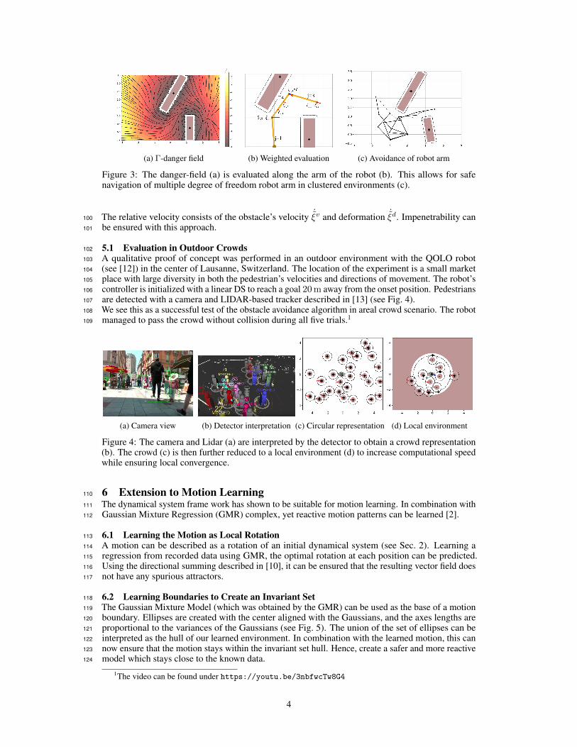
(a) Γ-danger field (b) Weighted evaluation (c) Avoidance of robot arm

Figure 3: The danger-field (a) is evaluated along the arm of the robot (b). This allows for safenavigation of multiple degree of freedom robot arm in clustered environments (c).

The relative velocity consists of the obstacle’s velocity ˙̃ξv and deformation ˙̃

ξd. Impenetrability can100

be ensured with this approach.101

5.1 Evaluation in Outdoor Crowds102

A qualitative proof of concept was performed in an outdoor environment with the QOLO robot103

(see [12]) in the center of Lausanne, Switzerland. The location of the experiment is a small market104

place with large diversity in both the pedestrian’s velocities and directions of movement. The robot’s105

controller is initialized with a linear DS to reach a goal 20 m away from the onset position. Pedestrians106

are detected with a camera and LIDAR-based tracker described in [13] (see Fig. 4).107

We see this as a successful test of the obstacle avoidance algorithm in areal crowd scenario. The robot108

managed to pass the crowd without collision during all five trials.1109

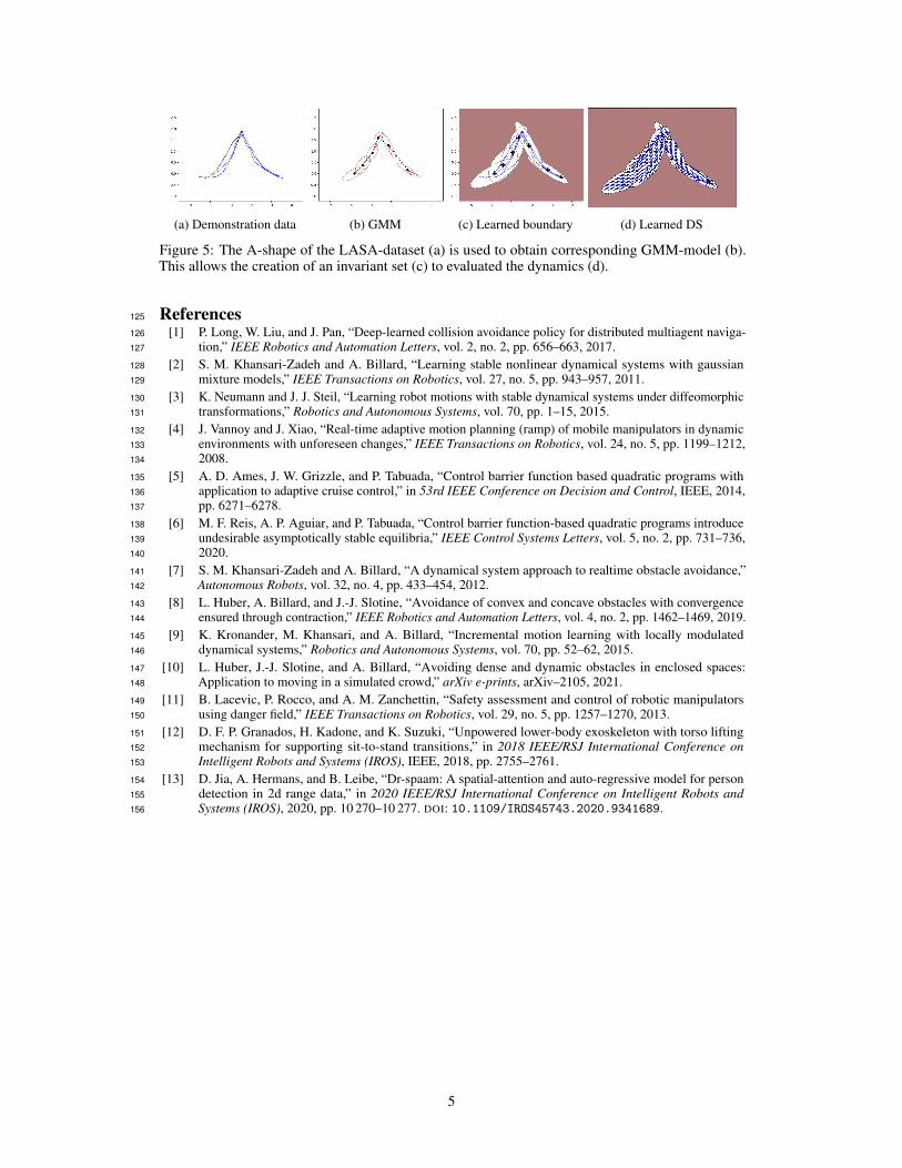
(a) Camera view (b) Detector interpretation (c) Circular representation (d) Local environment

Figure 4: The camera and Lidar (a) are interpreted by the detector to obtain a crowd representation(b). The crowd (c) is then further reduced to a local environment (d) to increase computational speedwhile ensuring local convergence.

6 Extension to Motion Learning110

The dynamical system frame work has shown to be suitable for motion learning. In combination with111

Gaussian Mixture Regression (GMR) complex, yet reactive motion patterns can be learned [2].112

6.1 Learning the Motion as Local Rotation113

A motion can be described as a rotation of an initial dynamical system (see Sec. 2). Learning a114

regression from recorded data using GMR, the optimal rotation at each position can be predicted.115

Using the directional summing described in [10], it can be ensured that the resulting vector field does116

not have any spurious attractors.117

6.2 Learning Boundaries to Create an Invariant Set118

The Gaussian Mixture Model (which was obtained by the GMR) can be used as the base of a motion119

boundary. Ellipses are created with the center aligned with the Gaussians, and the axes lengths are120

proportional to the variances of the Gaussians (see Fig. 5). The union of the set of ellipses can be121

interpreted as the hull of our learned environment. In combination with the learned motion, this can122

now ensure that the motion stays within the invariant set hull. Hence, create a safer and more reactive123

model which stays close to the known data.124

1The video can be found under https://youtu.be/3nbfwcTw8G4

4

(a) Demonstration data (b) GMM (c) Learned boundary (d) Learned DS

Figure 5: The A-shape of the LASA-dataset (a) is used to obtain corresponding GMM-model (b).This allows the creation of an invariant set (c) to evaluated the dynamics (d).

References125

[1] P. Long, W. Liu, and J. Pan, “Deep-learned collision avoidance policy for distributed multiagent naviga-126

tion,” IEEE Robotics and Automation Letters, vol. 2, no. 2, pp. 656–663, 2017.127

[2] S. M. Khansari-Zadeh and A. Billard, “Learning stable nonlinear dynamical systems with gaussian128

mixture models,” IEEE Transactions on Robotics, vol. 27, no. 5, pp. 943–957, 2011.129

[3] K. Neumann and J. J. Steil, “Learning robot motions with stable dynamical systems under diffeomorphic130

transformations,” Robotics and Autonomous Systems, vol. 70, pp. 1–15, 2015.131

[4] J. Vannoy and J. Xiao, “Real-time adaptive motion planning (ramp) of mobile manipulators in dynamic132

environments with unforeseen changes,” IEEE Transactions on Robotics, vol. 24, no. 5, pp. 1199–1212,133

2008.134

[5] A. D. Ames, J. W. Grizzle, and P. Tabuada, “Control barrier function based quadratic programs with135

application to adaptive cruise control,” in 53rd IEEE Conference on Decision and Control, IEEE, 2014,136

pp. 6271–6278.137

[6] M. F. Reis, A. P. Aguiar, and P. Tabuada, “Control barrier function-based quadratic programs introduce138

undesirable asymptotically stable equilibria,” IEEE Control Systems Letters, vol. 5, no. 2, pp. 731–736,139

2020.140

[7] S. M. Khansari-Zadeh and A. Billard, “A dynamical system approach to realtime obstacle avoidance,”141

Autonomous Robots, vol. 32, no. 4, pp. 433–454, 2012.142

[8] L. Huber, A. Billard, and J.-J. Slotine, “Avoidance of convex and concave obstacles with convergence143

ensured through contraction,” IEEE Robotics and Automation Letters, vol. 4, no. 2, pp. 1462–1469, 2019.144

[9] K. Kronander, M. Khansari, and A. Billard, “Incremental motion learning with locally modulated145

dynamical systems,” Robotics and Autonomous Systems, vol. 70, pp. 52–62, 2015.146

[10] L. Huber, J.-J. Slotine, and A. Billard, “Avoiding dense and dynamic obstacles in enclosed spaces:147

Application to moving in a simulated crowd,” arXiv e-prints, arXiv–2105, 2021.148

[11] B. Lacevic, P. Rocco, and A. M. Zanchettin, “Safety assessment and control of robotic manipulators149

using danger field,” IEEE Transactions on Robotics, vol. 29, no. 5, pp. 1257–1270, 2013.150

[12] D. F. P. Granados, H. Kadone, and K. Suzuki, “Unpowered lower-body exoskeleton with torso lifting151

mechanism for supporting sit-to-stand transitions,” in 2018 IEEE/RSJ International Conference on152

Intelligent Robots and Systems (IROS), IEEE, 2018, pp. 2755–2761.153

[13] D. Jia, A. Hermans, and B. Leibe, “Dr-spaam: A spatial-attention and auto-regressive model for person154

detection in 2d range data,” in 2020 IEEE/RSJ International Conference on Intelligent Robots and155

Systems (IROS), 2020, pp. 10 270–10 277. DOI: 10.1109/IROS45743.2020.9341689.156

5