A Uni ed Approach to Model Selection and Sparse Recovery ...

A Unified Approach to Model Selection and Sparse

Recovery Using Regularized Least Squares

Jinchi Lv and Yingying Fan

Presented By: Weiyu Li, Wei Kuang and Han Chen

2018.11

SICA 1

Focus

1. Model selection:

Weak oracle property: exponential growth of dimensionality (p) with

respect to sample size (n).

2. Sparse recovery:

SICA: a family of penalties between l0 and l1.

SIRS: sequentially and iteratively reweighted squares algorithm.

3. Regularized Least Square (RLS) with concave penalties

SICA 2

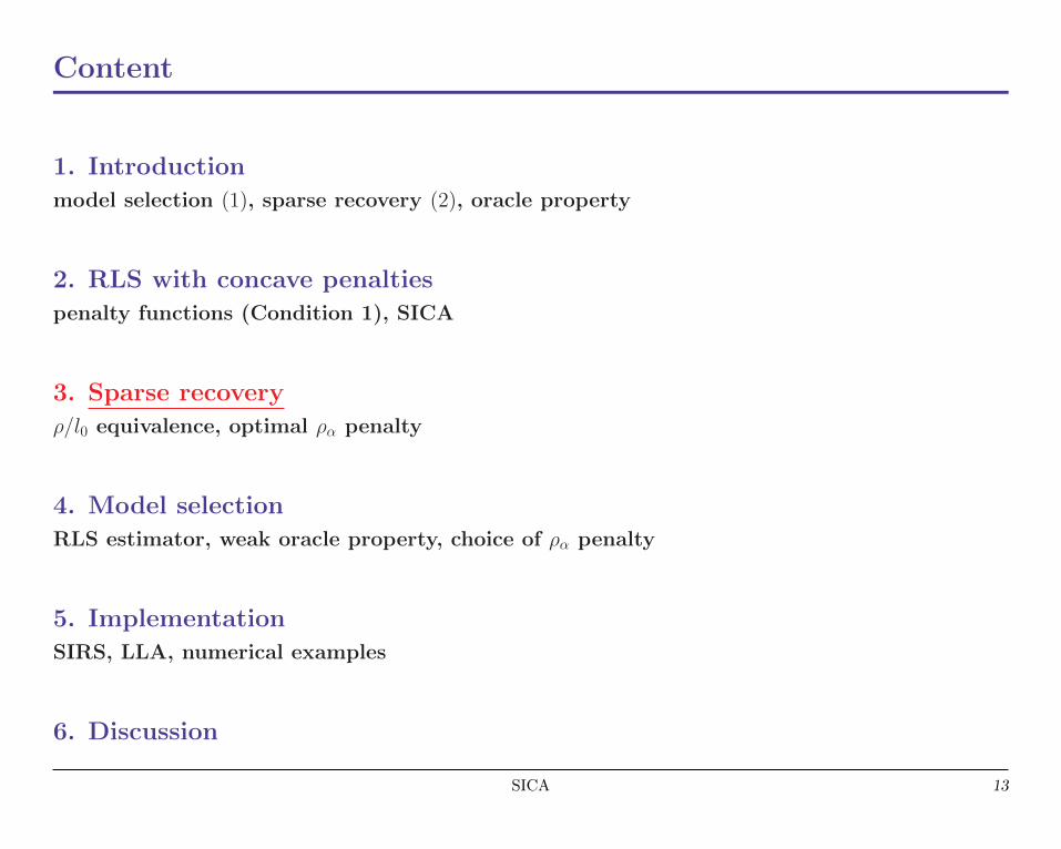
Content

1. Introduction

model selection (1), sparse recovery (2), oracle property

2. RLS with concave penalties

penalty functions (Condition 1), SICA

3. Sparse recovery

ρ/l0 equivalence, optimal ρα penalty

4. Model selection

RLS estimator, weak oracle property, choice of ρα penalty

5. Implementation

SIRS, LLA, numerical examples

6. Discussion

SICA 3

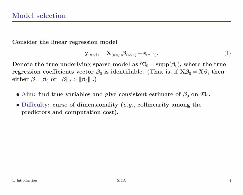
Model selection

Consider the linear regression model

y(n×1) = X(n×p)β(p×1) + ε(n×1). (1)

Denote the true underlying sparse model as M0 = supp(β0), where the true

regression coefficients vector β0 is identifiable. (That is, if Xβ0 = Xβ, then

either β = β0 or ‖β‖0 > ‖β0‖0.)

• Aim: find true variables and give consistent estimate of β0 on M0.

• Difficulty: curse of dimensionality (e.g., collinearity among the

predictors and computation cost).

1. Introduction SICA 4

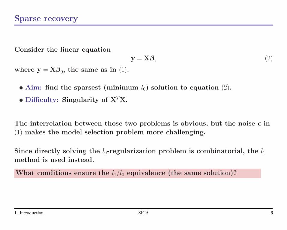
Sparse recovery

Consider the linear equation

y = Xβ, (2)

where y = Xβ0, the same as in (1).

• Aim: find the sparsest (minimum l0) solution to equation (2).

• Difficulty: Singularity of XTX.

The interrelation between those two problems is obvious, but the noise ε in

(1) makes the model selection problem more challenging.

Since directly solving the l0-regularization problem is combinatorial, the l1method is used instead.

What conditions ensure the l1/l0 equivalence (the same solution)?


Oracle property [2] and weak oracle property

An estimator β̂ has the oracle property, if

(1) P(β̂Mc

0= 0)n→∞−→ 1,

(2) β̂M0is asymptotically unbiased and normal-distributed with the

information bound attained.

An estimator β̂ has the weak oracle property, if

(1) P(β̂Mc

0= 0)n→∞−→ 1,

(2) l∞ loss (‖β̂ − β0‖∞) is bounded with a sequence converging to 0.

Consequently from the theorems in [1] and [2], β̂ with (weak) oracle

property is asymptotically consistent.


Content

1. Introduction




3. Sparse recovery


4. Model selection


5. Implementation


6. Discussion

SICA 7

RLS - problems rewriting

For sparse recovery (2), consider

min

p∑j=1

ρ(|βj|), (3)

s.t. y = Xβ,

where ρ(·) : [0,∞)→ R is a penalty function.

For model selection (1), consider

minβ∈Rp

1

2‖y −Xβ‖2

2 + Λn

p∑j=1

pλn(|βj|), (4)

where Λn ∈ (0,∞) is a scale parameter, pλn(·) is a penalty function with

regularization parameter λn ∈ [0,∞).

Abbreviate ρ(t) = ρ(t;λ) = λ−1pλ(t) for t ∈ [0,∞), λ ∈ (0,∞).

Later we will analyze solutions of (3) with special penalties and then let

λ→ 0+ to solve the sparse recovery problem.

2. RLS with concave penalties SICA 8

Penalties

• l0 penalty: ρ(t) = I(t 6= 0).

• l1 penalty: ρ(t) = t.

• l2 penalty: ρ(t) = t2.

l0: discontinuous, impractical in high-dim.

l2: analytically tractable, but non-sparse solutions.

l1: biased, not an oracle (not always a true solution).

Hereafter, consider concave penalties.


Condition 1

penalty function ρ(t) is increasing and concave in t ∈ [0,∞), and has a

continuous derivative ρ′(t) with ρ′(0+) ∈ (0,∞). If ρ(t) is dependent on λ,

ρ′(t;λ) is increasing in λ ∈ [0,∞) and ρ′(0+) is independent of λ.

For example, the SCAD [2] penalty satisfies Condition 1.

Figure 1: An illustration for SCAD penalty.


SICA: a family of penalties

However, consider another family of penalties {ρa : a ∈ [0,∞]} given by

ρa(t) =

(a+1)ta+t =

(t

a+t

)I(t 6= 0) +

(aa+t

)t, a ∈ (0,∞)

I(t 6= 0), a = 0

t, a =∞, (5)

which are called smooth Integration of counting and absolute deviation

(SICA) penalties.

ρa penalties with a ∈ (0,∞] satisfies Condition 1, and more strictly with

a ∈ [a0,∞), they give estimators satisfying unbiasedness, sparsity and

continuity, where a0 = λ +√λ2 + 2λ is a constant depending on λ.

Notice that the maximum concavity of ρa penalty is

κ(ρa) := supt∈(0,∞)

−ρ′′a(t) = 2(a−1 + a−2),

therefore parameter a controls the maximum concavity of ρa.

0 = κ(ρ∞) < κ(ρa) < κ(ρ0+) =∞.


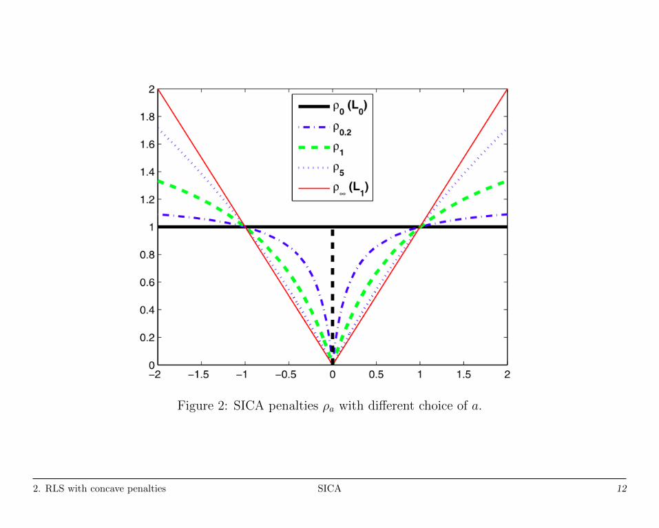
Figure 2: SICA penalties ρa with different choice of a.


Content

1. Introduction




3. Sparse recovery


4. Model selection


5. Implementation


6. Discussion

SICA 13

Sparse recovery

Recall that the sparse recovery problem is [cf. (2)]

y = Xβ.

Consider the case of q := p− rank(X) > 0. We expect an equivalence to [cf. (3)]

min

p∑j=1

ρ(|βj|),

s.t. y = Xβ.

Denote A = {β ∈ Rp : y = Xβ}, thus the solution of (2) can be rewritten to

β0 = arg minβ∈A‖β‖0. (6)

β0 is unique under mild assumptions. For example, ‖β0‖0 <spark(X)

2 in [3].

3. Sparse recovery SICA 14

l2 penalty

Naively, (6) can be relatex to

β2 = arg minβ∈A‖β‖2 = (XTX)+XTy,

which is nonsparse, thus far away from β0.

Thereafter, we are curious about the ρ/l0 equivalence, where the penalties ρ

satisfying Condition 1 are more general than the l1 penalty (lasso).


ρ/l0 equivalence

Notations

pλ(t) =λρ(t), t ∈ [0,∞),

ρ̄(t) :=sgn(t)ρ′(|t|).

For SICA penalties ρa, we have

ρ′a(t) =

{a(a+1)(a+t)2

, t ∈ [0,∞), a ∈ (0,∞)

1, a =∞,

ρ̄a(t) =

{sgn(t)a(a+1)

(a+t)2, a ∈ (0,∞)

sgn(t), a =∞.

Instead of directly solving the minimization problem (3), consider the ρ-RLS

problem [cf. (4)]

minβ∈Rp

1

2‖y −Xβ‖2

2 + Λn

p∑j=1

pλn(|βj|)

with regularization parameter λn = λ ∈ (0,∞) and then let λ→ 0 + .


Theorem 1 (RLS solution of (4))

Assume that pλ satisfies Condition 1 and β̂λ∈ Rp with Q = XT

M̂λXM̂λ

non-

singular, where λ ∈ (0,∞) and M̂λ = supp(β̂λ). Then β̂

λis a strict local

minimizer of (4) with λn = λ if

β̂λ

M̂λ=Q−1X̂T

M̂λy − ΛnλQ

−1ρ̄(β̂λ

M̂λ), (7)

‖zM̂cλ‖∞ <ρ′(0+), (8)

λmin(Q) >Λnλκ(ρ; β̂λ

M̂λ), (9)

where z = (Λnλ)−1X̂TM̂λ

(y − X̂M̂λβ̂λ), λmin(·) denotes the smallest eigenvalue of a

given symmetric matrix, and κ(ρ; β̂λ

M̂λ) is the local concavity of ρ at β̂

λ

M̂λ.

From Theorem 1, we have an explicit solution of problem (4). Letting

λ→ 0+ provides a sufficient condition for the ρ/l0 equivalence, which is

stated in the following theorem.


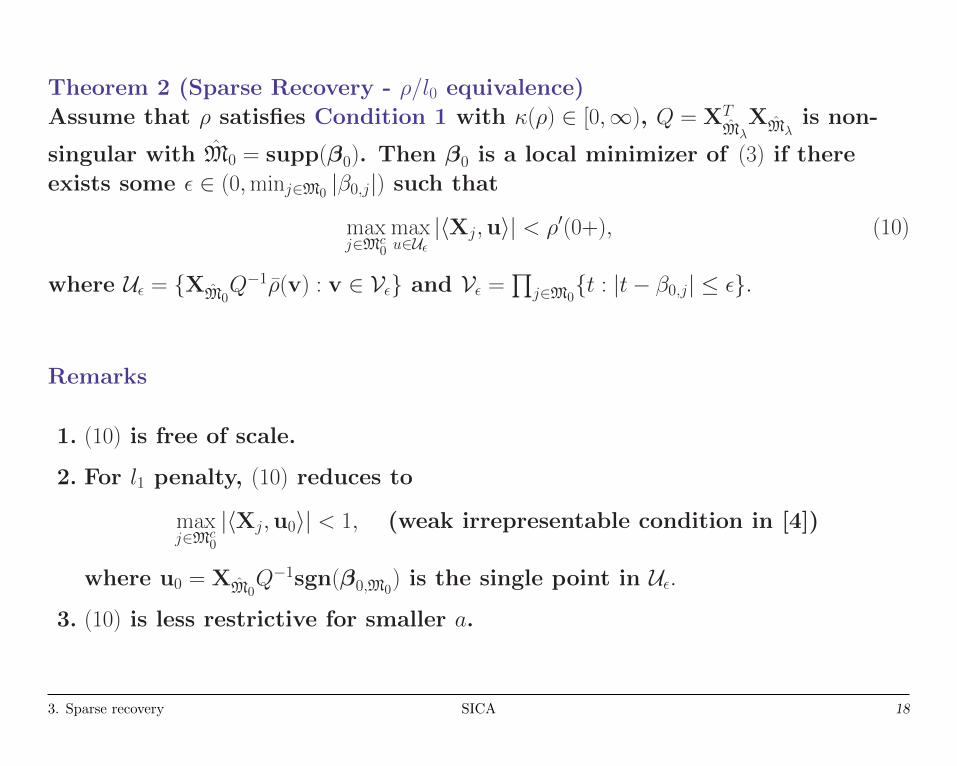
Theorem 2 (Sparse Recovery - ρ/l0 equivalence)

Assume that ρ satisfies Condition 1 with κ(ρ) ∈ [0,∞), Q = XTM̂λ

XM̂λis non-

singular with M̂0 = supp(β0). Then β0 is a local minimizer of (3) if there

exists some ε ∈ (0,minj∈M0 |β0,j|) such that

maxj∈Mc

0

maxu∈Uε|〈Xj,u〉| < ρ′(0+), (10)

where Uε = {XM̂0Q−1ρ̄(v) : v ∈ Vε} and Vε =

∏j∈M0{t : |t− β0,j| ≤ ε}.

Remarks

1. (10) is free of scale.

2. For l1 penalty, (10) reduces to

maxj∈Mc

0

|〈Xj,u0〉| < 1, (weak irrepresentable condition in [4])

where u0 = XM̂0Q−1sgn(β0,M0

) is the single point in Uε.

3. (10) is less restrictive for smaller a.


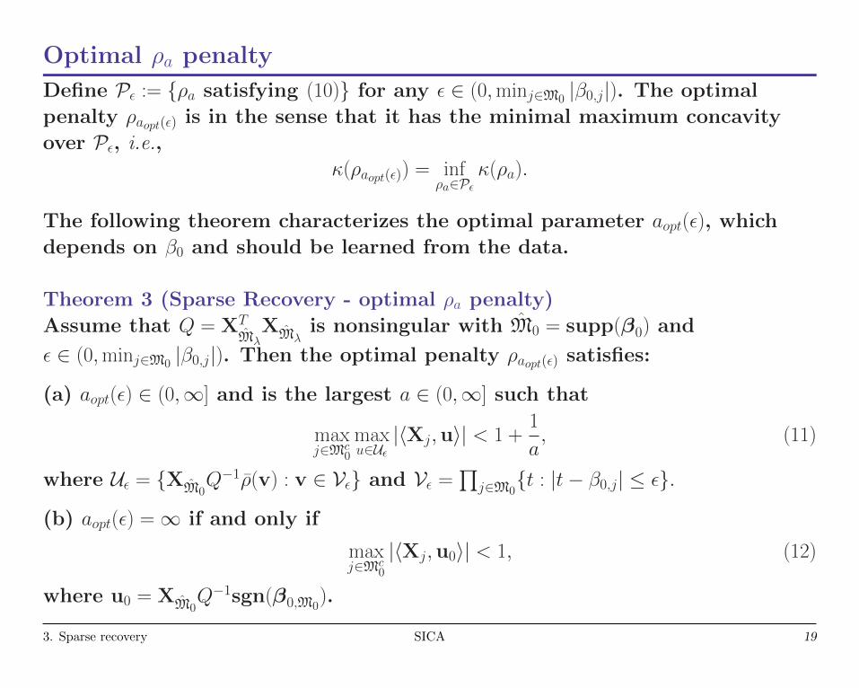
Optimal ρa penalty

Define Pε := {ρa satisfying (10)} for any ε ∈ (0,minj∈M0 |β0,j|). The optimal

penalty ρaopt(ε) is in the sense that it has the minimal maximum concavity

over Pε, i.e.,

κ(ρaopt(ε)) = infρa∈Pε

κ(ρa).

The following theorem characterizes the optimal parameter aopt(ε), which

depends on β0 and should be learned from the data.

Theorem 3 (Sparse Recovery - optimal ρa penalty)

Assume that Q = XTM̂λ

XM̂λis nonsingular with M̂0 = supp(β0) and

ε ∈ (0,minj∈M0 |β0,j|). Then the optimal penalty ρaopt(ε) satisfies:

(a) aopt(ε) ∈ (0,∞] and is the largest a ∈ (0,∞] such that

maxj∈Mc

0

maxu∈Uε|〈Xj,u〉| < 1 +

1

a, (11)

where Uε = {XM̂0Q−1ρ̄(v) : v ∈ Vε} and Vε =

∏j∈M0{t : |t− β0,j| ≤ ε}.

(b) aopt(ε) =∞ if and only if

maxj∈Mc

0

|〈Xj,u0〉| < 1, (12)

where u0 = XM̂0Q−1sgn(β0,M0

).


Content

1. Introduction




3. Sparse recovery


4. Model selection


5. Implementation


6. Discussion

SICA 20

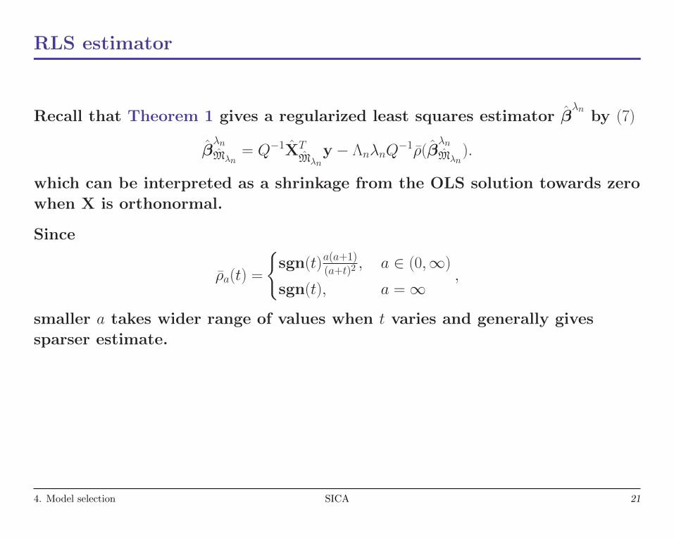
RLS estimator

Recall that Theorem 1 gives a regularized least squares estimator β̂λn

by (7)

β̂λnM̂λn

= Q−1X̂TM̂λn

y − ΛnλnQ−1ρ̄(β̂

λnM̂λn

).

which can be interpreted as a shrinkage from the OLS solution towards zero

when X is orthonormal.

Since

ρ̄a(t) =

{sgn(t)a(a+1)

(a+t)2, a ∈ (0,∞)

sgn(t), a =∞,

smaller a takes wider range of values when t varies and generally gives

sparser estimate.

4. Model selection SICA 21

Weak oracle property

As mentioned in the introduction, weak oracle property means: (1) sparsity

and (2) consistency under l∞ loss, which is weaker than the oracle property.

Theorem 4 (Weak oracle property)

Using penalties satisfying Condition 1, under mild conditions and

p = o(uneu2n/2), there exists a regularized least squares estimator β̂

λnwith

regularization parameter λn, such that with high probability, β̂λn

satisfies:

(a) (Sparsity) β̂λnM̂c

0= 0;

(b) (l∞ loss) ‖β̂λnM̂0− β0,M̂0

‖∞ ≤ h = O(n−γun),

where γ ∈ (0, 12] and the divergent sequence{un} depend on X, the penalty ρ

and the local concavity. Consequently, ‖β̂λn − β0‖2 = Op(

√sn−γun), where

s = ‖β0‖0 is the sparsity.

Remarks:

1. If the local concavity is small, un = o(nγ) and thus log p = o(n2γ).

2. In classical settings, γ = 12. Thus the consistency rate of β̂

λnunder the

l2 norm is Op(√sn−1/2un), which is slightly slower than Op(

√sn−1/2).

4. Model selection SICA 22

Content

1. Introduction




3. Sparse recovery


4. Model selection


5. Implementation


6. Discussion

SICA 23

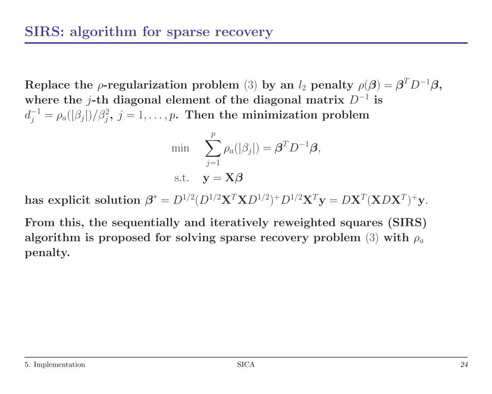
SIRS: algorithm for sparse recovery

Replace the ρ-regularization problem (3) by an l2 penalty ρ(β) = βTD−1β,

where the j-th diagonal element of the diagonal matrix D−1 is

d−1j = ρa(|βj|)/β2

j , j = 1, . . . , p. Then the minimization problem

min

p∑j=1

ρa(|βj|) = βTD−1β,

s.t. y = Xβ

has explicit solution β∗ = D1/2(D1/2XTXD1/2)+D1/2XTy = DXT (XDXT )+y.

From this, the sequentially and iteratively reweighted squares (SIRS)

algorithm is proposed for solving sparse recovery problem (3) with ρapenalty.

5. Implementation SICA 24

Algorithm 1. SIRS

Input: sparsity level S, the number of iterations L, the number of sequential

steps M ≤ S and ε ∈ (0, 1).

1. Set k = 0.

2. Initialize β(0) = 1 and set l = 1.

3. Set β(l) ← DXT (XDXT )+y with D = D(β(l−1)) and l← l + 1.

4. Repeat step 3 until convergence or l = L + 1. Denote the resulting vector

as β̃.

5. If ‖β̃‖0 ≤ S, stop and return β̃. Otherwise, set k ← k + 1 and repeat steps

2-4 with β(0) = I(|β̃| ≥ γ(k)) + εI(|β̃| < γ(k)) and γ(k) the kth largest

component of |β̃|, until stop or k = M . Return β̃.

The convergence of SIRS has not been proved in [1], but they gave a

proposition in the paper, which states that:

if p > n, ‖β0‖0 <spark(X)

2 = n+12 , then β0 is a fixed point for SIRS separated from

other fixed points.


*LLA: local linear approximation

For the objective function∑p

j=1 ρa(|βj|) in (3), a naive but efficient idea is to

approximate it by a first-order expansion

p∑j=1

[ρa(|β(0)

j |) + ρ′a(|β(0)j |)(|βj| − |β

(0)j |)

].

LLA [5] is based on the approximation and solves the weighted lasso in

one-step

minβ∈Rp

1

2‖y −Xβ‖2

2 + Λnλn

p∑j=1

wj|βj|,

where wj = ρ′a(|β(0)j |) = a(a + 1)/(a + |β(0)

j |)2, j = 1, . . . , p.


Numerical examples

Sparsity recovery:

• Compare SIRS with LLA.

• Evaluation: Success percentage of recovering β0.

Table 1: Success percentages of different choices of penalties in recovering β0 under different correlation rusing SIRS and LLA algorithms.

Penalties SIRS LLAr = 0 r = 0.2 r = 0.5 r = 0 r = 0.2 r = 0.5

l1 11% 8% 4% - - -ρ5 19% 12% 8% 28% 26% 20%ρ2 50% 37% 32% 53% 40% 34%ρ1 63% 58% 51% 57% 46% 43%ρ0.2 76% 70% 61% 27% 24% 17%ρ0.1 77% 68% 63% 7% 10% 8%ρ0.05 71% 68% 61% 2% 3% 2%ρ0 19% 51% 48% - - -


Model selection:

• Cross-validation for optimal parameters.

• Compare: Lasso, SCAD, MCP [6], SICA. Implemented by LARS [7] for

Lasso, and LLA for others.

Figure 3: Comparison of l1, SCAD and MCP penalties. The plot on the right shows their derivatives.

• Evaluation: the prediction error (PE, by an independent test sample of

size 10, 000) and the number of selected variables (#S).


Table 2: Meas of PE and #S over 30 simulations for all methods with different noise levels σ.Lasso SCAD MCP SICA

σ = 0.5 PE(×10−3) 37.52 8.98 8.89 10.34#S 10.43 8.43 8.40 7.00

σ = 0.1 PE(×10−2) 13.49 8.04 7.93 9.43#S 11.13 8.80 8.70 7.87

Figure 4: Boxplots of PE and #S over 30 simulations for all methods with different noise levels σ. Toppanel is for PE and bottom panel is for #S.


Content

1. Introduction




3. Sparse recovery


4. Model selection


5. Implementation


6. Discussion

SICA 30

Discussion

• Multivariate response

• Directly solving l0 penalty

• Distributed optimization

• ......

6. Discussion SICA 31

REFERENCES REFERENCES

References

[1] Lv, J., and Fan, Y. (2009). A unified approach to model selection and

sparse recovery using regularized least squares. Ann. Statist. 37(6A),

3498-3528.

[2] Fan, J. and Li, R. (2001). Variable selection via nonconcave penalized

likelihood and its oracle properties. J. Amer. Statist. Assoc. 96, 1348-1360.

MR1946581

[3] Donoho, D. L. and Elad, M. (2003). Optimally sparse representation in

general (nonorthogonal) dictionaries via l1 minimization. Proc. Natl. Acad.

Sci. USA 100, 2197-2202. MR1963681

[4] Zhao, P. and Yu, B. (2006). On model selection consistency of Lasso. J.

Mach. Learn. Res. 7, 2541-2563. MR2274449

[5] Zou, H. and Li, R. (2008). One-step sparse estimates in nonconcave

penalized likelihood models (with discussion). Ann. Statist. 36 1509-1566.

MR2435443

[6] Zhang, C.-H. (2007). Penalized linear unbiased selection. Technical report,

Dept. Statistics, Rutgers Univ.

[7] Efron, B., Hastie, T., Johnstone, I. and Tibshirani, R. (2004). Least

angle regression (with discussion). Ann. Statist. 32 407-451. MR2060166

SICA 32

A Uni ed Approach to Model Selection and Sparse Recovery ...

Documents

Transcript of A Uni ed Approach to Model Selection and Sparse Recovery ...