7 A A1 I 4 88 YALE A4IV NEW HAVEN CT DEPT OF COMPUTER SCIENCE F16 12/1

ITERATIVE SOL.UTION OF INDEFINITE SYMMETRIC SYSTEMS BY METHODS U-CTYC(U)U NL_ OCT 81 Y SAAO N00011-76-C-0277

WICLASSIFIED TR-212 N

Eh~hEEE~h2

1 2.2

L4.0 12.01.8

11111 L25 j.4 1 .6

MICROCOPY RESOLUTION TEST CHART

I TI

YALE UNIVERIT

I, DPARTENT F CMPUTR SCENC820 04 "41

Z79RATIVE SOLUTION OF INDEFINITE 87NMB'IhCSYSUNS By NUMODS usnIs CWLUCSKAL 0

FOLYNWDIA q OVU TW0 DISJOINT XNMYALS

Y. SAAD

Technical Report # 212October 12, 1981

This work was supported in part by the U.S. Office of Naval Research undergrant N000014-76-C-0277 and in part by NSF Grant.

tiT~bui~S -

Abstract

It is shown in this paper that certain orthogonal polynomials over two

disjoint intervals can be particularly useful for solving large

symetric indefinite linear systems or for finding a few interior

eigenvalues of a large symtric matrix. There are several advantages

of the proposed approach over the techniques which are based upon the

polynomials having the least uniform norm in two intervals. While a

theoretical comparison will show that the norms of the minimal

polynomial of degree n in the least squares sense differs from the

minimax polynomial of the same degree by a factor not exceeding

422(n+l/ 0 the least squares polynomials are by far easier to compute

and to use thanks to their three term recurrence relation. A number

t of suggestions will be made for the problem of estimating the optimal

parameters and several numerical experiments will be reported.

...........o

?NTIS GRU&1DTIC TASUnanauun d

LD i,.tr _but 1. On ...Avajlgb*At+"y Codes

Dista ptciBI.i .... !i l::l - . ,.

iCOPY

2

This paper is concerned with the solution of large indefinite linear systems

A x f. The number of effective Iterative methods for treating such problems is

limited. An obvious possibility is to solve the normal equations Ax - A f by any

available method for solving positive definite systems but this is not recommended

in general as it increases the amount of work and above all squares the original

condition number. Perhaps the beat known contribution in the field was made by

Paige and Saunders who adapted the Conjugate Gradient method to indefinite

systems [8]. There have also been a few attempts towards the generalization of

the Chebyshev iteration algorithm (also called Stiefel Iteration) to the

indefinite case by Lebedev [6],Roloff [10] and de Boor and Rice [4]. These works

focus on the difficult problem of finding a polynomial of degree n such that

Pn(O)=1 and having least uniform norm in two intervals containing the elgenvalues

I of A but not the origin. Like in the positive definite case, such polynomials are

the best for making the residual norm small in a certain sense in the Richardson

iteration:

zn+1=Xn rn

where vn is the n root of the polynomial and r is the residual of z n There

are, however, some serious drawbacks of this approach one of the most important

being that the mini-nax polynomial is rather difficult to obtain numerically.

Moreover the above Richardson iteration is unstable in general,

At this point one might ask whether it is essential to use the minimax

polynomial. Perhaps the most attractive property of the Chebyshev polynomials is

its three term recurrence formula which enables one to generate, In the positive

definite case, a sequence of approzinmato solutions to the linear system which

satisfy a three term recurrence. As pointed out by do Door and Rice [4], it seems

•1 4 . x I '_..21L -, tZ ,,. , , ,

3

unfortunately impossible to exhibit a three term recurrence for the minimax

polynomials over two intervals.

Nevertheless a natural alternative considered in this paper is to construct a

sequence of polynomials satisfying pn(0)-1 and which minimize an L2 norm

associated with a certain weight function over the two intervals. Such polynomials

are easy to compute and can be obtained via a sequence of polynomials satisfying a

three term recurrence. Moreover it will be shown that their uniform norm in the

two intervals is comparable within a factor of 2(n+l) 1/2 with the norm of the

minimax polynomial if n is the degree of both polynomials. We will call

Generalized Chebyshev Iteration (GCI) the iterative method which at each step

yields a residual vector of the form rn=pn(A)r0 where Pn is the minimal

polynomial. There are several other applications of the minimal polynomial in

addition to the Generalized Chebyshev Iteration. First, a block version of the

alSorithm can be formulated. It is essentially a generalization of the block

Stiefel algoritbm described in [111 and is particularly suitable for parallel

computation. Secondly there are various ways of using the minimal polynomials for

computing eigenvectors associated with interior eigenvalues. For example one can

easily adapt the subspace iteration method (see [91) to interior eiSenvalues. A

few of the possible generalizations and extensions of the basic Generalized

Chebyshev Iteration will be briefly outlined but we will not attempt to describe

them in detail.

Section 2 describes polynomial iteration for solving linear systems. In

section 3 we will deal with the orthogonal polynomials over two intervals and will

introduce the minimal polynomial. Section 4 covers the application of the minimal

polynomials to the solution of indefinite systems while section 5 outlines their

application to the interior igenvalue problems. Zn section 6 a umber of

practical details, concerning in particular the estimation of the optimal

4

parameters, are given. Finally some numerical experiments are reported in section

7 and a tentative conclusion is drawn in the last section.

2. fljZam itLeation In IJAMU hAlMLJ

Consider the N x N linear system

A x f (2.1)

where A is a nonsingular symetric matrix. Let x0 be any initial guess of the

solution x and r0 the corresponding initial residual r0 - f - A z0 . Polynomial

iteration methods are methods that provide approximate solutions xn whose

residuals rn satisfy:

rn = Pn ( A ) r0 (2.2)

where Pn is a polynomial of degree n, often called the residual polynomial. We

only consider methods in which xn is given by

xn+1 ' xn + anUn (2.3)

where un , the direction of search, is a linear combination of the previous

residuals. In this case it can easily be shown by induction that the polynomial pn

satisfies the condition Pn(0) 1.

If r0 is written in the elaenbasis (ul 1 ,N of A as

N0 4 = 1 "1u

then obviously the Euclidean norm of rn is

N 2 12 (2

Ilrnl1 I I PUO) 4, 2 (2.4)i-1

where the X ' a are the eigenvalues of A.

ILL--

[S

Equation 2.4 suggests the general principle that if we want the residual norm

lin1l to be small, we must find a polynomial satisfying pn(O) = 1 which is small

in some set containing the eigenvalues of A. One way of choosing a residual

polynomial which is small in a set containing the spectrum is to take among the

polynomials satisfying pn (0) = 1 the one which has the least uniform norm in that

set. When the matrix A is positive definite its eigenvalues can be included in

one single interval [a,b] not containing the origin and the polynomial having

least uniform norm in [a,b] can easily be expressed in terms of the Chebyshev

polynomials. This is the essence of the Chebyshov semi iterative method [5].

When A is not positive definite, i.e. when it has both positive and negative

eigenvalues, then its spectrum can be included in two disjoint intervals [a,b],

[c,d] with b < 0 < c , and the polynomial having having least uniform norm in

[a,b] U [c,d] can no longer be easily expressed. Lebedev [6] considered this

problem and gave an explicit solution to it for the very particular case when the

two intervals [a,b] and [c,d] have the same length. Lebodev does not however give

any suggestion for the general case and de Boor and Rice (41 showed how to

practically obtain the polynomial of minimal uniform norm in two disjoint

intervals. There remains however several serious difficulties with the use of

these minimax polynomials which render the method unattractive and unreliable.

Firstly the computation of the minimax polynomial can be particularly difficult

and time consuming. Secondly once the minimax polynomial is available one must

perform the Richardson iteration:

SXi+ 1 = Ii + Ci ri (2.5)

where the v 'a are the inverses of the roots of the minimax polynomial. These

roots should therefore be computed before 2.5 is started but this can be done at a

negligible cost. The main disadvantage of 2.5. however, lies in its unstability.

This can easily be understood by deriving from 2.5 the equivalent equation for the

6

residual vectors

ri+liri -l A ri - (I - iA)ri

which shows that

ri+ (1 -i+ A)(I - -i A ) (I-co A) r0 (2.6)

Although the final residual rn should be small in exact arithmetic, the

intermediate residuals ri can be very large as is easily seen from 2.6 and this

may cause unstability in iteration 2.5. Reordering of the parameters T might be

used to achieve a better stability [1] although this does not seem to constitute

a definitive remedy. Note also that the computation of the roots of the minimal

polynomial can be itself an unstable process. Finally another drawback with the

use of the minimax polynomial is that if a polynomial of degree m is used then the

intermediate vectors xi with i~m do not approximate the exact solution x. Only the

last vector Im does in theory. The implication of this is that one cannot stop the

process and test for convergence before the m steps are all performed. If the

accuracy is unsatisfactory after the m steps, one has the alternatives of either

recomputiang another polynomial with different degree and restart 2.5 or perform

again a steps of iteration 2.5 with the same polynomial.

It will be seen that all of the difficulties mentioned above can be avoided

by using polynomials that are small in the two intervals in the least squares

sense i.e. polynomials which minimise the norm with respect to some weight

function w(x). This brings up orthogonal polynomials in two disjoint intervals.

-4 7

7

3. Oktoaau s ol nuamilsA&a In Dsji Rnt IntlaLs

3.1. Basis defialtIons ad notation

In this subsection we will describe general orthogonal polynomials in two

disjoint intervals. Let (a,b). (cd) be two open intervals such that b ( 0 <

c. The assumption that the origin lies between the two intervals is not essential

for this subsection. We consider a weight function w(x) on the interval (a,d)

defined by

Wl(z) for x e (ab)

w(Z) = w2 (m) for x e (c,d)

0 for x C (b,c)

where wl(x) and w2 (x) are two nonnegative weight functions on the intervals (a,b)

and (c,d) respectively. The inner product associated with w(x) will be denoted by

(. ., i.e.:

(f,8> = fJ f(x)g(x)w(x)dx

or:

(f,> -A f(z)g(z)wl(z)dx + _ f(x)g(x)w2 (z)dx (3.1)

The norm associated with this inner product will be denoted by 1I.11c i.e.

IlfIl = (f,f>1l 2 . We will often use the notation (f,g>1 and (f,8>2 for the first

and the second term of the right member of 3.1 respectively.

The theory of orthogonal polynomials shows that there is a sequence (pn) of

polynomials which is orthogonal with respect to (.,.>. All of the properties of

the orthogonal polynomials in one interval hold for the case of 2 intervals,

provided we consider these polynomials as being orthogonal on (ad) rather than on

(ab)U(c€d). For example although we cannot assert that the roots are all in

[ab]U[c,d]. we know that they belong to the interval [a,d]. Cases where one root

is inside the interval (bc) can easily be found. But the fondamental three term

recurrence relation which holds for all sequences of orthogonal polynomials is

obviously valid. Thus the polynomials pn satisfy a recurrence of the form:

Pn+lPn+l() = (X-Cn)Pn (x) - Pn~n-l(x) (3.2)

with

an (xPn>pn ) (3.3)

11 iiM <llc > 1/2 (34)on+ W n+l C Pn+lPu+l

where

;n+1 x) = (x-a n)pn(x) - PnPnSl(Z) (3.5)

One important problem considered in this paper is to find weight functions

for which the coefficients alp Pi are easy to generate and to propose algorithms

which generate them. Before entering into the details of this question in the

next subsection let us briefly outline how these polynomials may be obtained.

First select two weight functions wI and w2 such that for each of the intervals

(ab) and (cd) the orthogonal polynomials considered separately are known. Then

express the orthogonal polynomials in (ab)U(c~d) in terms of the orthogonal

polynomials in (ab) and in terms of the orthogonals polynomilas in (c,d). Te thus

obtain two sets of n+l expansion coefficients expressing the polynomial pn Using

these coefficients we are able to obtain the recurrence parameters an and n of

* equation 3.2 by formulas 3.3 and 3.4. Hence the two sets of expansion coefficients

can now be updated by use of 3.2 to yield the expansion coefficients of the next

polynomial Pna+ etc... Next the details of this procedure will be developed for a

Judicious choice of wI and w2 .

9

3.2. Generalisd Chebysh.v polynomials.

Let c1=(a+b)/2, c2=(c+d)/2 be the middles of the two intervals and

d1=(b-a)/2, d2=(d-)/2 their half widths. Consider the following weight

functions:

wl(x) - (2/) [d12- (X-C1)

2 ]-1/2 for x e (ab) (3.6)

S w2(x) = (2/) [d2 (X-C2)2 1-1/2 for x e (c,d) (3.7)

The orthogonal polynomials in (a,b) with respect to the weight function w1 can be

found by a simple change of variables to be:

T [(X-C 1 (3.8)

where T is the Chebyshev polynomial of the first kind of degree n. Likewise inn

the second interval (c,d) the orthogonal polynomials with respect to w2 are the

polynomials:

T [(i-c2 )/d2 (3.9)

We are interested in the polynomials p n(x) which are orthogonal in

(a,b)U(c€d) with respect to the weight function w(x) defined by w1 in (ab) and

in (c,d). In order to generate these polynomials we simply express them in terms

of the polynomials 3.8 in (aob) and in terms of the polynomials 3.9 in (c.d) as

follows:

nPn(z)_ I . n) T i[ (U-)/d1 (3.10)

i0

PnW) I 6 (n) Ti[lX 1()/d ] (3.11)n -02 2

The following proposition will enable us to compute the coefficients an and

Pn+1 given the ys and the Vs

I-7

- - -

10

rpjjsiti L.: Lot n k 3M Ixaamial of dAee n havingL fllo2yUin

eznansions in £aIb) &nd £,dA

np(x)= I= YiTi[UX-C1)/d 1 I for z e (a,b) (3.12)

i=0n

p(x)=-1 6oiTi[(X-c 2 )/d21 for x e (c,d) (3.13)

Set:

' U-1 n-1

(Pnp> 1: 21 + a2 (3.14)

(xp,p> =c I I + 2 + dl 1 +d2'2(.5

Proof: Consider 3.14 first. From 3.1 and 3.12, 3.13 we have:

n n

(Pop>-<i=1 Y T [(X-C )/d] "iy1 iT i[ (x-c1)/dl] )

Using the change of variable y (X-C1)/d I and the orthogonality of the Chebyshev

polynomials we obtain

2 n_ 2(P , P>I 1 = 2 y o + '1fi= 1

By the same transformations we would obtain (pop>2 = a2" Hence (pp> - <pep>1 +

(P-0)2 ' a1 + e2 which is precisely 3.14.

In order to prove 3.15 consider <xp,p)1 and <xp,p>2 separately. We have:

I X-Cl< Xp , p >1 d1< I < >1 + a 1 P >1 (3.16)

The first inner product can be transformed as follows:

11

1-01 1-

p.- p° >1 " < Ti[! d 1], Y Ti[ 1]l >

where 2 stands f or 2 . By the change of variables y Ithis simplifies into

- 2 +1

=X p . P> f +1 [ y Ti(Y) ]2 (1-y2 )11/2 dy (3.17)

Using the relations:

y Ti(Y) =1 [TI+I(y) + TiilY)

y To(y( ) T (y)

we find

2i y Ti(y) - ! TO(y) + ( + 2/2) Tl(y)

+ 1(yi-1 + vi+1 ) Ti(y) +... l'(yn-l + yn+i) Tn(Y)

For convenience Tn+l is set to zero. Replacing this in 3.17 and using the

orthogonality of the Chebyshev polynomials with respect to the weight function

(1-y2) 1 / 2 we get

( 1p - p >1 : !Y170 so+lYlY2/

1 1i(Tl+l+yt-1)ytst +"'+ 2(yn+1 + ¥n-1)TnSn

with s o = 2 and a, = 1 for i 0 . This finally yields

(Slp , P > V1-1

and by 3.14

XP , p >1 - clal + d1:1 (3.18)

A similar calculation would give

12

(zp.P>2 = e2@2 + d2?2 (3.19)

Adding 3.18 and 3.19 finally yields the desired result 3.15.

Q.E.D.

Once the parameters an and 0n+I are ocomputed by an appropriate use of 3.14

and 3.15, it is possible to generate the next orthogonal polynomial Pn+l (). The

next proposition provides a simple way of obtaining Pn+l when the expansions 3.10

and 3.11 are used.

P ropsition 3.2: e ( ) .... be th e qj Ot *hnmi polynomials

derived from .2 . jhe t he a(n) the YnnuI M I,1

satisfv the reurnc reai,

(n+l) d1 (n) (n) W( (n-1)Pn+li = j i(lYYi+l ) + i2,3....n+l (3.20)

Ni" the initial com:i2Da*

(n+l) (n) + ( n(n)- (n-i)Pn+lO - dly1 (3.21)

(n+l) (n).1 (n)1 W (n) (n-1)n+lyl d: 1l T (Y T2 2 + (01l'an )Y1 - Pn¥l (3.22)

Srelation anlsu Io 3-.LO &a AR whc jL, A& re e kX jg ui j At hod

foer .k 6'..

PrgoL From 3.2 we have

- 7(n)~n~lPn+l (z ) = (x-an) I1 T I(X-C1 )/d11 - An Y T(n-l) TI(_l)/dl

Using again the change of variable y-(z-o1)/dI for convenience we get

An+lPn+l ' (dl+Y+l-n) I y n) Ti(y) - On 1 Y(i1) T i(y)

Noticing that y T (y) - I( T11 (y) + Ti+I(y)) when i I 1 and y T0(y) - Tl(y)

we obtain:

13

d-(n)Pnl d~ -1 T (y) + Ti 1(y) +(€I- n) -_ T( T(Y)2n 1 n~l = 1 1Ti+1

(n-l) T (y)-n i-T i

with the notational convention T -1 TI . Therefore

,l id(n) (n) n) Tl(Y)~nj.~nl 1 1 0 + 2/2 1

+ 1(y (n) + (n)) T (Y) I +(c1 a n) ( T (Y)

(n-i) Ti(Y )

with the conventions stated in the proposition. Returning to the x variable gives

the desired expansion of Pn+l in the form 3.10 and 3.11 and establishes the

result.

t Q.E.D

The results of the previous two propositions can now be combined to provide

an alSorithm for computing the sequences of orthogonal polynomials. The idea of

the algorithm is quite simple. At a typical step the polynomial p is available

through its expansions 3.10 and 3.11 so one can compute an by formula 3.14. Then

we can compute the expansion coefficients of ;n+l using proposition 3.2. Finally

Pn+1 is obtained from 3.4 and 3.14 and Pn+1 is normalized by Pn+l to yield the

next polynomial Pn+l" This describes schematically one step of the algorithm

given below. A notational simplification is achieved by introducing the symbol

defined by

i-n i-n1 ai - 2 2 + a, (3.23)L=0 1=0

AOK I

Ca g iU t enalized Ckaknknz P nan als

1. IflALM. Choose the initial polynomial p0 (x) in such a way that

14

(0) (0) (0) (0) 1 (0) (0)YO :=u0 1 :~2 -Y D Z 2 : moo:=

2. Xtuats. For n-0 ,1,2....,n do

Compute % by formula 3.15:

(n) (n) (n) (n)an := cla1 +022 +dI 1 + d 2 2

- Compute expansion coefficients of Pn+i by formulas 3.20 - 3.22 andtheir analogue for the 6 'a.

-(n~) .(n). (n). (n-1)YO :-d 1 , c1 -a ny0 -pnO

-(n+l) (n) 1 (n) (n) (n-i)Y1 :-d l(YO '-2Y2 )+(Cl1 -a n)T1 -Pnl'I

~(n+l) d (n) + (n) -+ ( (n-)2 :ly1-1 + + (-

i=2,3,. .. n+l

-(n+l) - (n) . ,(n) . (n-1)

0 261 +2 n 0-PnO

'(n+l) - -(n) 1 ,(n) . .. (n)-_ _(-l)&1 :=d2 (6 0 V22 )+(c2 " l -a)6 1 A n 6

(+l). d2 (n) () + - (n) .(n-1)S "'2 -1 + (2-n)6i -ai

1-2,3,.... n+1

- Compute 1; n+l1i by formula 3.14 and get Pn+1 by formula 3.4:

n+1-(n+) n+ 2

n±1:(n+l) E-(n+1)]2a2 i

iI1

-(n+1) -(n+l) 1/2P~n+ 1 := [ a 1 + a2

- Normalize Pn+l by An+1 to get a+1

Yi : t Uln+i 1 9 i : + 1

15

i 0 ... ,n 1

- Compute now a's and v s

(n+l) -(n+1) 2 (n+l) -(n+l) 2a1 : =i61 / Pu 2 2: 1 m /n 1i

(n+l) l) (n+l) (n+l) - (n+l) (n+1)1 : i T Il " 2 :W 1 i i6+11

At the nth stop of the algorithm one performs approximately 20(n+l)

arithmetic operations. Concerning the storage requirements, we must save the

(n) (n) (n-l) (n)coefficients y ,b0 as well as the previous coefficients Y0 , and 60

which means 4(n + 1) memory locations, if nax is the maximum degree allowed.maxnx

This suggests that, in practice nmax should not be too high. Note that restarting

could be used if necessary.

3.3. The minimal polynomial

Consider the orthonormal polynomial p3 of degree n produced by Algorithm 1.

According to section 2, an interesting approximate solution to the system A x = b

would be the one for which the residual vector rn satisfies:

rn = [pn(O)]- 1 pn(A) to

It is easily verified that such an approximation is given by

n = 10 + Onl( A ) r 0

where

Snal(x) - I P(O)]-1 [p(O) - pa(x)) / x (3.24)

Practically and theoretically however this approach faces several drawbacks.

First, it may happen that p3 (0) is zero or very close to zero. In that case the

thn approximation xn either is not defined or becomes a poor approximation to x(n

-- 6

16

respectively. Although this difficulty might be overcome by computing 1 n+l

directly from Xn I , this will not be considered.

A second disadvantage of using the orthogonal polynomials pn is that they do

not satify a suitable optimality property. More precisely the norm lIpiPn(O)I11

is not minimum over all polynomials of degree not exceeding n satisfying pn(0) =

1. This fact deprives us from any means of comparing the residual norms, and

above all does not ensure that the approximate solution Zn will eventually

converge towards the exact solution x.

These remarks lead us to resorting to the polynomial qn of degree n such that

qn (0) - 0 which minimizes the norm lql c over all polynomials q of degree j n.

Writing the polynomials q as q(x) - 1 - x s(x) where a is a polynomial of

degree not exceeding n-I, it is clear that our problem can be reformulated as

follows:

Find & volvnomial s e g MIg:

Ill-x Sn-l(x) II . IIl-x s(x)ll c . V a 4 pn-1 (3.25)

Here 1-is(x) denotes the polynomial q defined by q(x) 1- xp(z) rather than

the value of this polynomial at x.

From the theory of approximation it is known that the best polynomial sn-1

exits and is unique [3). Furthermore the theory of least squares approximation

0indicates that the solution a_ 1 must satisfy the equations:

C

(1-XS x s(x) >=O V a ePn-1 (3.26)

To solve 3.26 lot us aassume that we can find a sequence of polynomials

qjj0,l,..n-l,. such that the polynomials zqJ(z) form an orthonormal sequence

with respect to > , ). Then expressing a 1 as

N-1a

17

• n- z- q W xan1 j.O J J

we obtain from 3.26

l1j = <lD xqj(x) ) (3.27)

It turns out that the polynomials qj(x) can be obtained quite simply by an

algorithm which is nothing but algorithm 1 with a different initialization. This

is because we actually want to compute an orthogonal sequence of the form (xqn)

with respect to !he same weight function -Wa 88 before.

Practically we will have again to express the polynomials xqn(x) by two

different formulas as in subsection 3.2:

n+lxqn(x) = I0 a Ti(x), x e [a,b] (3.28)

i=0n~l (n)

-qnlx) -I16 Tx W x [ecd] (3.29)

Denoting by a and Pn the coefficients of the now three term recurrence whichn n

is satisfied by the polynomials qn we obtain:

n+1%+j() - U- Q); (x) -P%-.(x) (3.30)

which is equivalent to:

An+l xq3+1 (x) - (X- an) x%() -o' zq.,(x) (3.31)

The condition that the sequence ( zqj }J=0,.1..n.. Is orthonormal gives the

following expressions for a' and An:

'-(x (za), x > (3.32)n d'

p'' l- I1x+q IC - i(x - ,)ix%(x) - (3.%l3) ic3

It is clear froa the above formulas that the Algorithm for computing the

18

sequence zq (z) is essentially algorithm 1 in which the initialization is

replaced by a now one corresponding to the starting polynomial zqo (x) x instead

of P0 (x) - 1. Thus the orthogonal sequence xqn(x) replaces the sequence pn (x) of

algorithm 1.

We must now indicate how to obtain the expansion coefficients it of the

polynomial Sn* in the orthogonal basis q ). AccordinS to 3.27 we have

1 j= (1,xq )

Hence

tj " T0 ,zqj) 1 + (To0xq j 2

2( T(J ) +6# ( J ) (3.34)

Here we recall that the weight function w has been scaled such that

<T0 T0 >i-2. i- 1,2 and <T ,T i > 1 for JOO, i-1.2. As a consequence of 3.34 the

expansion coefficients in can be obtained at a negligible cost. Te can now write

down the algorithm for computing the orthogonal sequence qn(X). For simplicity the

prime symbols will be dropped.

1. JALtialLt . Choose the polynomial xqo(x) in such a way thatqOmcoustant and IlxIlc 1.

2 2 +2 2

t2:-2(c1 + c2 ) + d 2+d2

t:t21 / 2

T(0) :- ,6(0)..

0(0 ) :(0)T 1. 1 :-d o.

*(0) 2 2(0) 2 2a1 [- 201 4] d/t2,a 2 Me [22 + d2 11t2,

_____ lP- - :- -- e

____ _____-__-__7 2

19

(0) (0) (0) (0) : (0) 5(0)1 :2 0 1 2 0 1

2. Itera. For n-0,1,2 .... n, do

- Compute a by formula 3.15:n

(n) (n) (n) (n)a:cai +026 +d T + d2n 1 1 e202 +a11 22

- Compute expansion coefficients of q-+l by formula 3.20 - 3.22 andtheir analogue for the 6 '.

-(n+l). (n) (n) (n-i)Y :inly 1 +(c--eny 0 +(no

"(n+l) ()(. 1 (n (n) (n-1)¥1 1 l(T0 2" ) +tel-1muTI -Pny1

(n , (n) (n) (n) (n-1)Ti .So 2'lT -1$ + Tr +I") (cl-a n )Ti - .yi

i=2,3 .... ,n+2

-(n+l). - (n) u.. (,) (n-1)0 d261 +(c2-an 0 -P,6

-(n+l) (n) 1 (n) (a)- (n-1)81 :-d2 (60 V2Y 2)+(c2-%n)b 1 Pn 61

g(n+l) d Cn) Cu), + (n) (n-1)

i *-22°6-1 + 8i+l 2 n )i Pn i1

i-2.3.... ,n+2

- Compute II*.+l by formula 3.14 and get 0n+1 by formula 3.4:

-(n+l) n1 (7(n+l) 2 (n+l) n .1aI a- :. i r(nii2 i-i

'(n+1) -(n+l) 1/2'+I l 2

- Normalize 'n+l by A +I to Set

(n+l) ~;(,+1),, 6 "+ 1 ) : Innl l

i i P+I i i n+1

- Compute new a's and v's

20

(n+l). -(n+l) 2 (n+l) ~(n+l) 2a1 : =1 /n+1 a2 : n2 n+l

(n+l) ,(n+l) (n+l) (n+l): R _n1 i Yi+i 2 1 1 ,6( +l1i-On

Note that part 2( iterate ) is identical with part 2 of algorithm 1. It is

important to realize that the above algorithm does not yield directly the

polynomials qn but rather provides their expansion coefficients in terms of the

Chebyshev polynomials in the two intervals. In the subsequent sections we willC

need to generate the polynomial s (x). This can be achieved by coupling with partn

2 of the above algorithm the following

n~l [A n)qnlx ) _fnqnls)'n+

.(n+l) (n+l).1n+ l : M 2-( yo + 6 0

*n+l:1 'n + ln+lqn+1

starting with

.ox-/ , o(x) -My(0) + 6(0) 9, z0)

where t is defined in the initialization of the algorithm.

3.4. Comparison with the minimax polynomial.

The purpose of this subsection is to compare the norms of the minimal

polynomial described in the previous subsection and the polynomial having the

least uniform norm in [a,b] U [c,d] subjeot to the constraint p (0) - 1. We will

denote by Ilpil, the uniform norm on [a.b] U [c,d], that is:

ilpll,- mal Ip(z)Ize [a,bJU[o.dJ

C C

Let us denote by pn the minimal polynomial 1 - zsn-l(x) of degree n. defined

in section 3.3. and by p the polynomial of degree n of least uniform norm in

- '+ . . .. ' ' " ' + " i ' il I lin I il I I I l il l l ...n

- .. . - =

21

[a.b]U[c,d]. In other words we have

(3.35)

I1p:ll C Ilpll C, p CP

IIpI ll. Ilp1l, - p e P (3.36)n

Since P is a finite dimensional space all the norms of P are equivalent andn a

the following lma indicates precisely a comparison of the norms II.ll1 andI I*ll.

Lena 2A.: Let f be any polynomial of degree not exceeding n. Then:n

1) Ilf 11lC 2 Ilfnll. (3.37)

2) 1lfll 11 ln+l) 11211f n 11C (3.3s)

Proof. 1)

Ilfi c (f n f > <fn f >l+<fn" fn>2

b 2df(z) w(x) dx + f f2(x)w2(x) dx

n a 0

and finally

,Ilf I 1121nl lC J 4 lfnll!

which gives the first result by taking the square root of both members.

2)

Ilf 1lo max If (x)ixe [a)U[cdJ

Ilfl i.-max(max I yT IT[ x-oI )/d i ,max I 1 S iTi[ 1x-2)/d21 1)(3.39)xG[a,b) inO xO(c.dJ 1-O

22

where the y's and the 6's are the expansion coefficients of f in [a,b] and [cod]n

with respect to the polynomials 3.8 and 3.9 respectively. Usin$ the Schwartz

inequality we get

a

1 -r T 1 1 1 T'j[(x-c 1)/d 1 11 'i=O i=O 1=O

Hence

n ( 2 1/2

I tiTi[(X-Cl)/di]I S (n+l) 1 [1 y ] (3.40)i=O i=O

Likewise we can show that

T n12 2 1126iTi[(x-c 2 )/d 2 ]I .. (n+) 1 [ 2 i (3.41)

i=O i-0

Replacing 3.40 and 3.41 in 3.39 we get

n 212

hf n II. (n+l)1/2 max[ [ I211 I I i]

n 2 2 1/2S(n+l)~

j n+1) 1 1 2 [ _ , ' +6)i-0

- (n+l)112 Iltnll c

Here we have used the result of proposition 1 and the notation 3.24

Q.E.D

As an immediate consequence of 3.37 and 3.38 we can easily bound each of the

norms II I and J in terms of the other from the left and the right as inC i

the next inequalities:

(n+1)-11 2 wlall. IIfnIIC 2 Ilifll . (3.42)

_We now st ' th llmn - (o+1) I Ctio esame

We now state the main result of this subsection which compares with the same

23

norm the polynomials pn and p n

Theorem JA: Lot pn Ma pn be the mLmagx polynomial and I minimal polynomialn-

defined bj 3.35 and 3.36. Thent Ihe folig i .1alitieL hold.

I Ip:IcS11 S. n iipi c (3.44)

1 pll. Ipull. S 2(n+1) 1/2 11p .3.45)

Proof: We will only prove 3.44 as the proof for 3.45 is identical. The first

part of the double inequality is obvious by equation 3.34. The second part is a

simple consequence of lemma 3.3:

Ilp~ll C j (n+1)1/2 Ip-llo i(n+1)1/2 Ilp~ll.

S 2(n+1) 1/2 IIp.ll c

Q.E.D.

The meaning of the theorem is that the two polynomials pn and pn have a

comparable smallness in (a,b] U [cd]. This will have a quite interesting

implication for the numerical methods using polynomial iteration since it means

that we can replace the minimax polynomial by the least squares polynomial, which

is by far easier to generate and to use, and still obtain a residual norm which is

not larger than 2(n+l)1/ 2 times the norm corresponding to the minimax polynomial.

Note that there is no reason a priori why to compare the two polynomials with one

particular norm rather than the other. If the norm l IIC is chosen then the

polynomial p is smaller than the polynomial Pn while with the uniform norm then n

contrary is true. Whichever norm is used however, the two polynomials have a norm

1/2comparable within a factor not exceeding 2(n+l) 2

, as is asserted in the above

theorem.

24

4. A&n.lia to t Ig .jM solutiono g larg AaqAjti jylMa

4.1. The Generalised Chebyshe Iteration

Let us return to the system 2.1 and suppose that we have an initial guess x

of the solution. We seek for an approximate solution of the form

= x0 + an- (A)r0 (4.1)

where a is a polynomial of degree n-i and r0 the initial residual. The

residual vector r of x is given by

r = [I-As W(A)] r0 (4.2)

The development of the previous sections lead us to choose for an_1 the polynomial

n-l which minimizes Ili-xs(x)II C over all polynomials a of degree j n-l. From

subsection 3.3 we know that:

n-inl(x) = q 2 (x) (4.3)

where the qj (x) satisfy the recurrence 3.30 and

1j = 2(y (j) + 6 (J) )

Let us assume that the coefficients a, n as well as the y's and 6s are

known. Noticing that

11 1 qn+l (z)8n+l(x). Sn(X) + n+l

and letting u . qj( A )r0 , it is immediately seen from subsection 3.3 that the

approximate solution x can computed from the recurrence:

Tn = 2[y0(n) + 6 0(n) 1 (4.4)

Xf •n +1 :M xn +- in n n

25

u+1: [(A-a' I )u - P' u ] (4.5)n+ n+1 n n-

Clearly the coefficients P o a' and in can be determined at the same time asn n n

4.5 and 4.4 are performed. Therefore a typical step of the algorithm would be as

follows:

1. Compute a' , n nd the coefficients y'(n +l ), 61 (n+l) (see part 2 ofAlgorithm n.

2. Compute:

qn 2[y0 In ) + 80(n )] (4.6)

Xn+1 xn + jnUn (4.7)

Un+l i [(A-a' I )un - A' un-] (4.8)

Pn+l n n n-

We will refer to this algorithm as the Generalized Chebyshe, Iteration

alzorithm. Although we need not save the coefficients a' and P;, if a restartingnn

strategy is used in which the iteration is performed with the same polynomial it

will be more efficient to save the coefficients a' and P'.

Note that the multiplication by a scalar in 4.7 can be avoide4 ',-y using

instead of the vectors un the sequence of vectors u'n defined by:

up 1j uUn n qn

which can be updated in no more operations than are needed for u n

Each step of the above algorithm requires one matrix by vector

multiplication, 3N additions 3N multiplications and O(n) operations, at the nth

step. Four vectors of length N need to be stored in memory plus an extra O(n)

locations for the coefficients y amd 6. A feature of the Generalized Chebyshev

Iteration, which is particularly attractive in parallel computation is the absence

26

of any inner product of N-dimensional vectors.

4.2. A minimal residual type implementation

A look at the previous algorithm reveals a similarity with one of the various

versions of the conjugate gradient method which is described in [2]. One might

ask whether it is possible to provide a version of the method which resembles the

conjugate gradient or the conjugate residual method. We are about to show here

that the answer is yes and we will provide a method which is very similar to the

conjugate residual algorithm described in (2].

To be more specific we are looking for an iteration of the form:

In+, = xn + an Vn (4.9)

r n+l =r n -a n A wn (4.10)

iWn+ I ' n+i + bn w (4.11)

where the scalars a n b are some cowtficients that are computed in such a way

that at each step the residual r+ 1 is precisely the residual obtained by using

the minimal polynomial as described earlier.

There are two main reasons why such a new form of algorithm 3 might be sought

for. The first is that the above version is slightly more economical than

algorithm 3, specifically 4.9 to 4.11 can be performed with N less

multiplications. Note also that N less storage locations are required in the case

where the matrix by vector multiplication can be performed componentwise, i.e. if

the i-th component of Ax can be delivered cheaply for all i. The second reason for

looking for a version of the form given above is that the residual vector is

available at each step of the iteration.

27

Some theoritical background is necessary for the understanding of the

remainder of this subsection. The development of the conjugate gradient like

method to be presented is based on the simple remark that the approximate solution

xn belongs to the affine subspace xO+Kn where Kn is the so called Krylov subspace

spanned by r0 , Ar0 , A 2r0 ,... A -1r0 . Then the key observation is that there is

a one to one mapping between the subspace In and the space Pn- of polynomials of

deree not exceedng n-l. In effect for any element u of n of the form u = pr0

n-i+ ~r + .... + nlA r0 , we can associate the polynomial qu(t) = P0 + PIit +

.... +P nlt . Clearly the transformation which maps u into qu is an isomorphism

betweenKn and Pn-l" We now introduce a new inner product on Kn"

Definition: We will call Generalized Chebyshev inner product on K and will denoten

by (",)C the bilinear form defined by

(Uv)c = <(,v> (4.12)

where (.,.) is the the inner product on Pn- defined by 3.1. 3.6 and 3.7.

That this constitutes an inner product is an immediate consequence of the

isomorphism introduced above. There is no ambiguity in denoting again by tl.II C

the norm on K induced by this inner product . We then have the followingn

immediate result.

Polosition 4.1: A each L.te O2 the Geralized Chebvshev iteratiLon, the

j3iurjUint_ solution xn mi IM genalized thheyshe Agg" aama i Jf-Azx IC O1

th residual vectors zAz over aU vectors z o Kn

In other words we have:

1lf - A xll 1 lf - Ax IV x e Kn

The proof of the proposition is straightforward.

-- *- * - i..,

28

The most convenient way of deriving a version of algorithm 3 equivalent to

4.9-4.11 is to use a little analogy. Indeed since we want to minimize the residual

norm with respect to the generalized Chebyshev inner product 4.12 we can use an

adapted version of the minimal residual method which achieves the same goal with a

different inner product. The version given below is precisely an adaptation of the

conjugate residual method described in (2].

1. Initialize. Choose an initial vector x0 and compute r0=f-Ax0 , V0 r0 .

2. Iterate.

an :- (xqr qr /(1q xq%> (4.13)n n n n

1 x +A w n (4.14)

rn+1 :r n -anAw n (4.15)

b :- <xqr 'qr / zqr qr > (4.16)n+1 n+1 n n

wn+1 n+1 + bn wn (4.17)

qwn+1 qrn+1 + bn n4.18)

The computation of the inner products involved in 4.13 and 4.16 can be

carried out in a similar way as before by use of proposition 3.1 together with

expressions similar to 3.12, 3.13 for each of the polynomials qr and q1 but wen n

omit the details.

As with the conjugate residual method in the indefinite case, the above

algorithm faces a risk of breakdown in equation 4.16 because <xq ,qr > can ben n

equal to zero. We do not know under what circumstances the inner product

<xq ,q ) vanishes but our short experience is that this does not often happen.n r2

29

We will prefer algorithm 3 in general depite the little extra work and possibly

storage involved. Note that it is also possible to write a conjugate gradient type

method which would correspond to using as residual polynomial the orthogonal

polynomial of subsection 3.2, instead of the minimal polynomial of subsection 3.3.

4.3. A Block Generalization

A block algorithm can be derived from the Generalized Chebyshev Iteration

described above. The principle of the Block algorithm is similar to that of the

Block Stieffel iteration proposed in [111.

As shown in fig. 4-1 if an eigenvalue X i lies inside the interval [bc] then

p (i) is large in comparison with the other p ( ), with j 0 i.

As a consequence the residual rn - p(A)r0 will be mainly in the direction of

the eigenvector zi asociated with Xi" Therefore by a projection process theii

component of the residual in this direction can be eliminated leaving only the

small components in the directions z with j 0 i. Let us now assume that instead

of one eiSenvalue )IV we had m eigenvalues ,).i+1 ,..... i+z_ 1 inside [b,c], and

that we are performing m different Generalized Chebyshev iteration, using m

different starting vectors x0 1 ,x0 2 .. . ,0o"n. We can again make the same

argument: the residuals rn,k at the nth step will have their dominant componants

in the eigenvectors zi,zi+l,...,zi+ 1 and we can eliminate these components by

projecting onto the subspace spanned by (rn, )j-l,2,., m . It was shown in [11]

that in the positive definite case, the rate of convergence of the Block Stiefel

Iteration is in general substantially superior to that of the single vector

Stiefel Iteration.

The block algorithm is more particularly suitable for parallel computation

since the m Generalized Chebyshev iterations involved a. can be performed

30

MINIMRL POLYNOMIRL OF DEGREE 15

1.100 r- , .. .V.. . l. .. .I- I . .F I

0.600 -

-~ I

-

0. 100 -

-0.400--a & J-2.000 0.000 2.000 4.000 6.000

x

Figure 4-1: Minimal polynomial with some *igenvalues in [b~oJ

31

simultaneously. Ignoring the matrix by vector multiplication, intercommunication

between the processors is needed only when the projection process takes place,

which is infrequent. As mentioned earlier the fact that there are no inner

products of N dimensional vectors is a further advantage of this algorithm in

parallel computation.

4.4. A Priori Error Bounds.

We now establish an a priori error bound which will show that the Generalized

Chebyshev Iteration is convergent. We should emphasize however that the bound

given here is proposed for the sole purpose of demonstrating the global

convergence of the process and does not constitute a sharp error bound in general.

The next theorem is based on the following estimate of the residual norm

which is an immediate consequnece of lemma 3.3

Lema 4.2: At the n-th step of of the Generalized Chebyshev iteration the

residual norm r of the approximate solution x satisfies:n n

Ilr 11 J (n+)/2 II phll c II r11 (4.19)n

Proof: From equation 2.4 we have

lirnil 1 liroll max Ip(. L H

Therefore

lirn1l J Ilr 0 11 ln1 .

The result follows from inequality 3.37 of lemma 3.3.

Q.E.D.

Theoau 4_1: snuoose I tkt mila. oi A I& coained AR Lak ~ and ILo

• , - . . . ,,I. . . . . . . . . . . .. . . I I I I I I I i . . . .. . . . . . . .

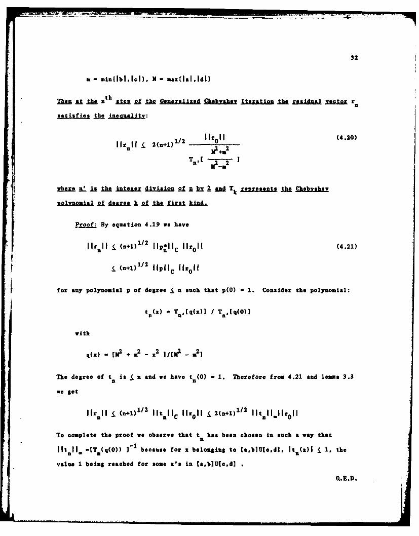
32

m = minulblhlcl) U - maz(lalldl)

Then at the n th 11M of the Generalized .akbzak u Itoation 2 h residual vector rn

satisfies As- ineguality:

l2( 3+ )1/2 li Oi (4.20)

where A. is the integer division of n b " & id Tk £WJA*&n1 thke ChkbX

polynomial of deLree k of jhe first kind,

Proof: By equation 4.19 we have

I lrn 11 (n+l)1/2 I11 ll (I I (4.21)i (n+1)1/2 IlplcIrl

C 0

for any polynomial p of degree j n such that p(O) - 1. Consider the polynomial:

t n(Z) - T f[q(x)] T n[q(O)]

with

q(z) _ ]i2 + m2 - x2 ]/[ 2 - 22 ]

The degree of t is I n and we have t (0) 1. Therefore from 4.21 and lemma 3.3n n

we get

Jirnal1 .j (In+l) 1 /2 i~tnJ11 C Iliol] . 21n+11 112 i~tnaJJ.J1rol

To complete the proof we observe that t has been chosen in such a way thatn

litnIla -[Ta(q(0)) 1-1 because for x belonging to [a.b]U[o,d], ltn(z)I j 1, the

value 1 being reached for some i's in Ca.b]Utc,d]

Q.E.D.

33

Note that ideally M2 and a2 are the largest and the smallest eigenvalues of

A 2 . Hence an interpretation of 4.20 is that n steps of our algorithm will yield a

residual norm not larger than 2(n+l) 1/2 times the residual norm obtained from

rn/21 steps of the classical chebyshev iteration applied to the normal equations

A2 x = A b. This result is however a pessimistic estimate as the numerical

experiments show.

S. ApplicatiLonto th EoautakoIa e lszanctozL assocLated Nt interior

Diuson ue •

Consider the eigenvalue problem

A z - X z (5.1)

where A is N dimensional and symmetric. When the desired eigenvalue X is one of

the few extreme eiSenvalues of A, there are a host of methods for solving 5.1,

among which the Lanczos algorithm appears as one of the most powerful. When X is

in the interior of the spectrum then problem 5.1 becomes more difficult to solve

numerically. The Lanczos algorithm often suffers from a slow rate of convergence

in that case and may require a number of steps as high as several times the

dimension N of A. A further disadvantage of this is that the Lanczos vectors must

be kept in secondary storage if the eigenveoctors are wanted. This might be

acceptable if a large number of eigenvalues are needed but when one only seeks for

a small number of them, possibly with a moderate accuracy, then the use of

techniques based upon subspace iteration should not be discarded.

We would like to indicate in this section how the polynomials described in

section 3 can effectively be used to ,btain approximations to eiSenveoctors

associated with interior eigenvalues. Consider an approximation to the eigenveoctor

z of 5.1 of the form:

34

Vn p (A) v0 (5.2)

where v0 is some initial approximation of z and pn a polynomial of degree

n. Writing v0 in the eigenbasis (z,)i.,,.. N as

Nv0 = i i

we obtain:

N= n 1Ci pn(oi) '1 (5.3)

which shows that if v is to be a good approximation of the eigenvector z then

every p n(Xj with j 0 1 must be small in comparison with pn (Xi . This leads to

seek for a polynomial which is small in [).,*) I]U[) ).N J and which satisfies1'i-i

pn(?i) = 1. In other words we need to find a polynomial of the form

-(x-)i )t nl(x-). i) which is small in these intervals in the least squares sense.

The simple change of variables t = x-X i trasforms this problem into the one of

subsection 3.3 thus providing an algorithm for computing an approximation to the

desired eigenvector associated with A.,. Note that in practice Xi is not available

and is replaced by some approximation p which is improved during the process. We

will find a polynomial in the variable t which corresponds to the operator A -I

i.e. the approximate eigenvector v will have the formn

vn P(A-pI) v0 I [ I - (A-pI) S*(A-I) ] v0

en

where p is the least squares polynomial obtained from algorithm 2 with

a I b- X - , € - d- XN4-p

where Xi-l and Xi+l are replaced by X- and X+ respectively.

An interesting problem which arises here is to estimate the interior

parameters b and a, or more precisely to refine dynamically a given pair of

35

starting parameters bc. This is discussed in the next section and a few

suggestions are given there.

An obvious extension of this algortibm which we omit to consider here is the

subspace iteration otherwise known as simultaneous iteration method ( See

e.g. [91)in which one iterates with a block of vectors simultaneously and uses the

Rayleigh Ritz projection approximations from the subspace spanned by the blocks.

6. Som rail considerations

6.1. Projection teohniques and the estimation of the optimal parameters.

Little was said in the previous sections about the determination of the

parameters a,bac,d. It is not often the case that these parameters are known

beforehand, and one has to provide means for computing them dynamically. This part

of the algorithm is a determinant factors of the efficiency. Let us recall that

a,d are ideally the smallest and largest eigenvalues 1 and "N of A, while b and c

should be equal to the eigenvalues ).- and X+ closest to the origin with X-(O and

X+>0. The smallest and largest eigenvalues X and XN are easier to estimate and

we have several ways of doing so, the simplest being perhaps the use of Gershgorin

disks. The use of the Lanczos algorithm is also particularly interesting since it

yields at the same time a good estimate of the parameters a,d and a fairly

accurate starting vector for the iteration(see e.g. [7]). It is a fact that the

eztremal parameters a.d which are easier to compute are also more important for

the convergence: if a is larger than I. or d is less than XN then there is a high

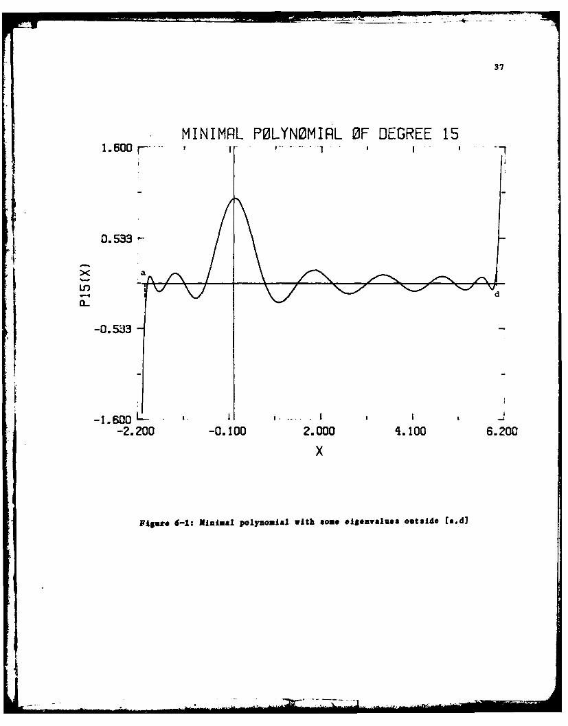
risk that the process will diverge. This is because outside the interval [a,d] the

residual polynomial can have huge values as is seen in figure 6-1. When this

happens however nothing is lost because we can stop and use the (huge) residuals

as approzimate eilenvectors associated with XI and XN thus providing more accurate

36

estimates of both a and d, with the help of the Rayleigh quotient. (See figure

6-1)

For the interior parameters b and c a projection technique based on a similar

principle can be developed. In effect if we start with two approximations b and c

such that b < X and c > X+,then as is seen from figure 4-1 the residual vectors

will have large components in the eigenvectors associated with the eigenvalues X

and X+ closest to the origin. A Rayleigh Ritz approximation can therefore by

applied to extract more accurate estimates of X- and X+ from two or more residual

vectors.

In fact a more complete procedure can be described as follows. Suppose that

we start with an interval [b,c] sufficiently wide to contain the eigenvalues X

and X. Then after a number of steps the residual vectors will give an accurate

representation of the eiSenspace corresponding to the eigenvalues contained in the

interval [I-,X+ 1. Therefore a projection process onto the subspace spanned by a

small number of successive residual vectors will provide not only a good

approximation of the eigenvalues I- and X+ ' but also the Rayleigh Ritz approximate

solution wiil be more accurate than the current approximation. In practice we

will iterate with a polynomial of fixed degree. We will orthonormalize the m

latest residuals where m is usually 5 or 6 (in order to have an accurate

representation of at least three eigenvectors ). Calling Q the orthonormal set of

vectors obtained from this orthogonalization. we compute the Ritz matrix T A Q

and its eigenvalues by e.g. the QR algorithm. We then compare tAw Ritz

eigenvalues thus obtained with those of the previous projection. After a certain

number of iterations some of the Ritz eigenvalues will converge to a moderate

accuracy (say to 2 or 3 digits of accuracy). As soon as an eigenvalue which

corresponds to either %-, or X+ converges, we replace b or c by that eigenvalue.

When both of the eigenvalues have converged, we replace the approximate solution

37

MINIMRL P0LYN0MIRL OF DEGREE 15

0.533

X ai

.- 4 d

-0.5 3

_1.600 _ I-2.200 -0.100 2.000 4.100 6.200

x

FiSuze 6-1: Minimal polynomial with some eiSeavaluea outside [ad]

38

by the Rayleigh Ritz approximation = X + I Ix 1 zr where the sun is over thenJ n

converged Ritz eigenvalues X and the z. are the associated approximate Ritz

eigenvectors. Recall that z1 is defined by z = Q.s1 where s is an eigenvector of

QT A Q associated with the Ritz value The effect of this important projection

step is to eliminate the (large) components of the residual in the direction of

the converged eigenvectors and is quite effective as will be seen in some

experiments described in section 7. A useful variation here is to use the latest

directions of search u instead of the latest residuals. We thus avoid to compute

residual vectors. The reason for this is that q n(A)r0 is a vector having large

components in the directions of the eigenvectors associated with the eigenvalues

nearest to zero. Our experience is that the results provided by the use of un

instead of r are often slightly better than those using the uneconomicaln

residuals.

The above process is even more efficiently implemented in a Block version.

because then we have a good approximation to several eigenvalues at the same time.

Note that in this case we need to have the interval [b,c] enclose at least m--i

eigenvalues if m is the dimension of the blocks.

The same projection technique as the one described above can be implemented

for the problem of computing an interior eiSenvalue X i and its corresponding

eigenvector. We will drop the subscript i in the following discussion. We are

again assuming here that we already know a good estimate of the extreme parameters

a, d and that we start with an interval [bc] sufficiently wide to contain the

eigenvalues X, X+ , and X-. Then after a number of steps of the iteration

described in section 5 the approximate eigenvectors will give an accurate

representation of the eigenspace corresponding to the eigenvalues contained in the

interval [b,c]. Hence a projection process onto the subspace spanned by a small

number of successive approximate eigenvectors will provide good approximations to

39

the eigenvalues X, X- and X+. Also the Ritz eigenvector will be a much better

approximation than the current approximation. Practically we will orthonormalize

the m latest approximations into the N x m orthonormal system Q. We then compute

the Ritz matrix QT A Q and its eigenvalues by e.g. the QR algorithm and compare

the Ritz eigenvalues obtained with those of the previous projection. As soon as- +

an eigenvalue which corresponds to either X, I , or X starts converging, we

replace p, b or c by that eigenvalue. When the three of the eigenvalues have

converged, we replace the approximate eigenvector by the Ritz vector z = Q s,

where s is the eigenvector of QT A Q associated with X. This process is tested in

an experiment in section 7.

6.2. Using high degree polynomials

One might ask whether it is possible to use high degree polynomials in

practice. Our experience is that despite the fact that we often encounter

underflow situations with high degree polynomials, if these underflows are handled

simply by replacing the underflowing numbers by zeroes, it is always better to use

a high degree polynomial than a low degree polynomial. This fact will be

illustrated in an experiment in the next section. Polynomials of degree as high

as 200 or 300 are quite useful for badly conditioned problems. We open a

parenthesis here to point out the following interesting observation. It has been

observed during the numerical experiments that the laLt coefficients 6(n)i " 7i

become tiny as J and n increase. This is the cause of the underflowing conditions

mentioned above. The practical consequences of this observation is that after a

certain number of steps we do not need to save those tiny elements. For high

degree polynomials this will result in a nonnegligible cut off in memory needs.

In fact a more important observation is that the coefficients % and Pn are

cyclically converging more precisely it seems that a3k+j is a converging sequence

for fixed J. The same phenomenon is true for the O's. A proof of this phenomenon

40

is not available however. As a consequence there is a hope that after a certain

step we can simply use the previous a's and P's thus avoiding further calculations

of these cofficients.

I

I " " ..........." '. ...-......-....-......" .............. .......' I I | l 1 ......I :

41

7. Numerical exerimeants

In this section we will describe a few numerical experiments and give some

more details on the pactical use of the Generalized Chebyshev Iteration. All the

experiments have been performed on a DEC 20, using double precision (unit roundoff

of order 10 - 1 7). Any mention to the Generalized Chebyshev iteration refers to

algortiha 3 rather than algorithm 4.

7.1. Comparison with 8730L

The SYNNLQ algorithm described in (8] and the various versions of it such as

MINRES [8] SYJOIK [21 all based on the Lanozos algorithm, are very probably the

best known iterative methods for solving large indefinite systems at the present

time so it is important to compare the performances of our algorithm with this

class of methods. We will mainly consider SYIMOK although some of the other

versions are slightly faster (but also slightly less stable). Although it is

difficult to make any definitive conclusion we will see that there are instances

where the Generalized Chebyshev iteration has a better performance than SYMLQ.

Table I shows the work per iteration and the storage requirements of both

algorithms when the number of nonzero elements in the matrix A is equal to NZ (We

have not counted the storage required for the matrix A). An obvious advantage of

the Generalized Chebyshev iteration is its low storage requirement. Note that with

algorithm 4 GCI would require 2N+NZ operations instead of 3N+4Z.

I Add/Mult-s I Storage I

I SXMLQ I 9N+N I 6N I

GCI I + I 4N-- -I -s +

Let us discuss the above table uder the assuptiom that NZ - S N, which

42

would correspond for example to applying the inverse iteration method to compute

an eigenvector of a Laplace operator. Then it is easily seen that our algorithm

becomes competitive if the number steps for GCI does not exceed 1.75 times the

number of steps required by SYO/IL. It is observed in practice that this ratio is

seldom reached. In fact as the next experiment will show, when the problem is well

conditioned i.e. when both b and c are not too small relative to a and d. then the

number of steps is not too different for the two algorithms. For the first

experiment we have chosen a diagonal matrix diag(X) where the eigenvalues Xi are

distributed uniformely in each interval [aob] and [c,d]. We have taken N-20,

a-2.0o. b=-0.5, c-0.5 and d-6.0. The eigenvalues )I are defined by:

define i, - r N(b-a)/(b-a + d-)1

for 1-1.2-.1: )i M a + (1-1).h 1 , with hi=(b-a)/(il-1) (7.1)

for i-i +l,...N: X c € + (i-1).h 2, with h2 -(d-c)/(N-i 1) (7.2)

TThe right hand side f has been taken equal to f A A e, where e -(ll,.l...I).

The initial vector was a random vector, the same for both SYI(LQ and GCI. The

Generalized Chebyshev iteration using the exact parameters a,b,cd is run with a

residual polynoomial of degree 25. The residual norms are plotted in figure 7-1

in logarithmic scale.This is done every 5 steps for a total of 75 steps. Observe

that the behaviors of both algorithms are almost identical.

This example shows the following interesting property: when the origin is

well separated from the spectrum the C-G like methods will converge with about the

same speed, but each step is more expensive as shown in table 1.

The next test compares the two algorithms in presence of a mildly badly

conditioned problem. We have taken the same example as above but the values of b

and c have been changed into -0.05 and 0.05 respectively, and N has been increased

43

GCI RND SYMMLQ2.000r i '

z 0.000- .c-

-2.000

*C)- "2C

tM

-,.0 z ,0.00 20.00 40.00 60.00 80.00

NUMBER OF STEPS

I SYMMLQ2 GCI

Figze 7-I: Comparison of SYIO.Q and GCI. H - 200, a-2.0,b--0.5,c-0.5,d6.0

44

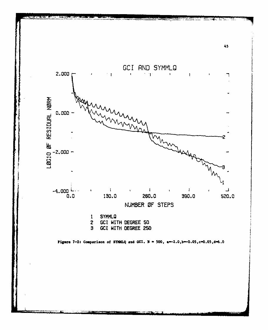
to 500. The sigenvalues Xi are defined again by 7.1 and 7.2. This is more

difficult to solve than our previous example. We have plotted in fig.7-2 the

logarithms of the residual norms for a total number of steps of 500. The inner

loop of GCI uses a polynomial of degree 250. (therefore 2 outer iterations were

taken.) The initial vector has been chosen randomly and has an initial residual

norm of.719 E+02. Although SYNNLQ requires loes steps here to achieve a reduction

of the residual norm by an order of 1.E-06, observe that in the beginning the GCI

has a better performance than ST10N". But as the number of steps approaches the

dimension N of A, we observe a speeding up of SYJ10LQ. Note that in exact

arithmectic SDIMLQ would have converged exactly at the 500-th steps. As a

comparison we plotted on the same figure the residual norms obtained with GCI

using a low degree polynomial. Observe the slowing down of GCI after 130 steps due

to the fact that the residuals start being in the direction of some eigenvectors.

This shows the superiority of using a higher degree polynomial when possible.

In the above experiments we have assumed that the optimal parameters a,b,c.d

are available. This is unrealistic in practice unless another linear system has

already been solved with the same matrix A. We would like next to show the

effectiveness of the projection procedure described in section 6. In the same

example of dimension 500 as above we have taken as extremal parameters the exact

values a and d. The interior parameters b and o were initially set to -0.15 and

0.15 respectively, instead of -0.05 and 0.05. We iterated with a polynomial of

degree 50. After each (outer ) iteration a Rayleigh Ritz step using the 10 latest

vectors uI as suggested in section 6 was taken. The convergence of the Ritz

eigenvalues is very slow in this example because the relative gap between the

sigenvalues of A is quite small. At the 9-th iteration no Ritz value has

converged to the demanded accuracy 10 - and it was decided to take a projection

step anyway with those sigenelements which have converged to a relative accuracy

of 0.2. The code then Save as eigeuvalues X--0.0504... and Xt+0.0507 and the

GCI RND SYMMLQ2.000

z

_j .000--D

0-4(nA

I I0.w3. 6. 9. 2.

NUBR FSTP1. SML

0i..072 oprsno YOL 130. 2G. 00 39-.Obn0.03,c520,m. .0

46

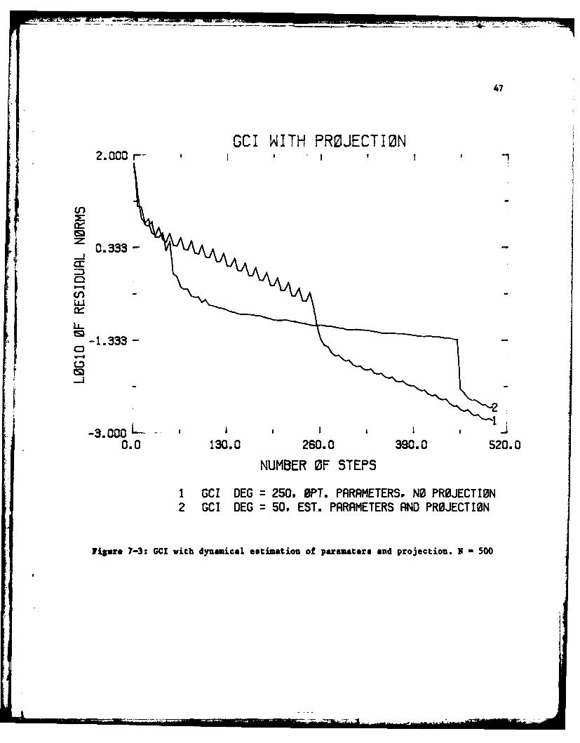
final (10-th) iteration was pursued with these values for b and c. Figure 7-3 is a

plot of the residual norms obtained with this technique together with those

previously obtained by using the exact parameters with a residual polynomial of

degree 250. It is remarkable that the final results are not too far from those

using the optimal parameters.

7.2. Computing interior eigenelements.

Consider the following N x N five-point discretization matrix

B -I 4 -11-I . 1-1 4 .

A I . . . withBi . . .

I .. 1- ... -1

-I B -1 4

and din(A) 150, dim(B) = 10

By Gershgorin's theorem all the eigenvalues of A lie in the interval [0,8].

Suppose that we would like to compute the eigenvalue nearest to the value 2.5 and

its corresponding eigenvector. Assuming that we do not have at our disposal any

estimate of the eigenvalues nearest to 2.5, we start the iteration described in

section 5 with p equal precisely to 2.5. Also as the first estimates of the

eigenvalues X + and ).-, the smallest eigenvalue at the right of I and the largest

eigenvalue at the left of X respectively, we take 3.0 and 2.0. The initial vector

v is generated randomly. After each outer iteration using a polynomial of degree

40 a projection step using the Iast 1U vectors is taken. The Ritz eigenvalues

are computed and compared with those obtained at the previous projection step as

described in section 6. When either of the oigenvalues corresponding to X+, X. or

X- has conversed to a relative accuracy of 10-3 then b, p, or c is replaced

accordingly. when the three olenvalues have converged the approximate

47

GCI WITH PROJECTION2.000-

O. 333-cc:

0-4Ln

u-

-1.333 -

-3.000 L0.0 130.0 260.0 390.0 520.0

NUMBER OF STEPS

1 GCI DEG = 250. OPT. PARAMETERS. NO PRBJECTION2 GCI DEG = 50. EST. PARAMETERS AND PROJECTION

Fiure 7-3: GCI with dynamical estimation of parameters and projection. N - 500

,. '. .' g ~ 7m - ,ai --- -.

48

eigenvector is replaced by the Ritz vector. Figure 7-4 shows 480 steps of such a

process (curve 1). Note the dramatic drop of the residual norm after the

projection process. Clearly such an improvement is not only due to the fact that

we now use better parameters b and c, but also to the fact that the current

approximate eigenvector is now purified from the components in the directions of

the undesired eigenvectors.

As a comparison the residual norms are plotted for the case where the exact

parameters 1- 2.436872, IL - 2.471196, and + 2.604246 are used. In this case

we iterated with a polynomial of degree 100 (Iteration with a polynomial of degree

40 gave much slower convergence) . Note that the process with orthogonal

projection is quite successful here since it does a better job than the algorithm

using the optimal parameters and a reasonably high degree polynomial.

8. Conclusion.

The numerical experiments suggest that the use of orthogonal polynomials for

solving indefinite linear systems as described in this paper can be effective

especially if one or more of the following conditions are met:

- The system to solve is not too badly conditioned.

- A moderate accuracy is required

- The operations y - A x are very cheap

- Several systems with the same matrix A are to solved. In that case theparameters are estimated only once .

The Generalized Chebyshev Iteration is a stable process and relatively high

degree polynomials can be used without difficulty to achieve a better performance.

In order to estimate the optimal parameters we resort to a projection procedure

which incidentally can also be used to improve the current approximate solution by

removing the undesired components.

49

INTERIOR EIGENELEMENTS BY GCI-'t " 'r 't,.

1.OE+O0

1. OE-01cr -CE

M 1.OE-O2c-

cm I.OE-03

_ I.OE-04i

CD -

1.OE-05 . ,

O.C 125.0 250.0 375.0 500.0

NUMBER OF STEPS

1 WrTH ESTIMRTISM OF PRRAMETERS AND PROJECTION2 WITH EXACT PARAMATERS AND NO PRSJECTIBN

118.1 7-4: Cospstia8 an interior siseapair with OC. N-150. . - 2.47119...

so

Several problems both theoretical and practical remain to be solved and more

numerical experience is needed before this class of techniques will become

reliable.

It is also hoped that besides their use in Numerical Linear Algebra, the

polynomials introduced in this paper will find applications in other fields of

numerical analysis such as in approximation of functions.

Acknowledsements. Most of the ideas of this paper were developed during a

visit at the University of California at Berkeley. I would like to express my

gratitude to Prof. B.N. Parlett for his hospitality at Berkeley and for valuable

comments about this work. I also benefited from helpful discussions with Stan

Eisenstat.

51

RitIKCIS

[1] R.S. Anderson G.H. Golub. Richardson's non stationary matrix iterativeprocedure. Technical Report STAN-CS-72-304, Stanford University, 1972.

[2] R. Chandra. Coniuxate Gradient Methods for Partial Differential Equations.Technical Report 129, Yale University, 1981. PhD Thesis.

[31 C.C. Cheney. Introduction to Annroximation Theory. Mc Graw Hill, N.Y.,1966.

[4] C. de Boor , J.R. Rice. Extremal Polynomials vith applications to Richardsoniteration for indefinite systems. Technical Report 2107, M.R.C., 1980.

[51 G.N. Golub , R.S. Varga. Chebyshev semi iterative methods successiveoverrelaxation iterative methods and second order Richardson iterativemethods. Numer. Hat 3:147-168, 1961.

[6] V.I. Lebedev. Iterative methods for solving operator equations vith aspectrum contained in several intervals. USSR Como Math Math Phvs9(6):17-24, 1969.

[7] D. A. O'Leary. Hybrid Coniugate Gradient alaorithms. Computer Science Dpt.Stanford University, Stanford, CA, 1976. PhD dissertation.

[81 C.C. Paige and M.A. Saunders. Solution of sparse indefinite systems oflinear equations . SIAN j. _9o NL Ir. Anal. 12:617-624, 1975.

[9] B.N. Parlett. The Imsetric Eigenalue Problem. Prentice Hall, EnglevoodCliffs, 1980.

[10] R. R. Roloff. Iterative solution of matrix equations for symmetric matricespossessina positive and negative eivenvalues. Technical Report UIUCDCSR-79-1018, University of Illinois, 1979.

[111 Y. Saad , A. Sameh. A parallel Block Stiefel method for solving positivedefinite systems. In M.H. Schultz, Editor, Proceedings of the EllipticProblem Solver Conference, Academic Press, 1980, pp. 405-412.

IA