This article appears in IEEE Transactions on Industrial Electronics, 2021. DOI: 10.1109/TIE.2021.3102431

A Two-Layer Near-Optimal Strategyfor Substation Constraint Management

via Home BatteriesIgor Melatti, Federico Mari, Toni Mancini, Milan Prodanovic, Member, IEEE, and Enrico Tronci.

Abstract—Within electrical distribution networks, sub-station constraints management requires that aggregatedpower demand from residential users is kept within suitablebounds. Efficiency of substation constraints managementcan be measured as the reduction of constraints violationsw.r.t. unmanaged demand. Home batteries hold the promiseof enabling efficient and user-oblivious substation con-straints management. Centralized control of home batter-ies would achieve optimal efficiency. However, it is hardlyacceptable by users, since service providers (e.g., utilitiesor aggregators) would directly control batteries at userpremises. Unfortunately, devising efficient hierarchical con-trol strategies, thus overcoming the above problem, is farfrom easy. We present a novel two-layer control strategy forhome batteries that avoids direct control of home devicesby the service provider and at the same time yields near-optimal substation constraints management efficiency. Oursimulation results on field data from 62 households in Den-mark show that the substation constraints managementefficiency achieved with our approach is at least 82% of theone obtained with a theoretical optimal centralized strategy.

NOMENCLATURE

s EDN substationTs set of time slots for substation sU set of houses (users)t time slot (element of T )u house (element of U )Tu set of time slots for house u; note that, for all notation de-

pending on an house index u, if the house is understood,u is not shown

Tu,P set of time slots in Tu in which the EV is plugged-inon house u

τl duration (in minutes) of time slots in Ts

Authors Melatti, Mancini and Tronci are with the Sapienza Universityof Rome, via Salaria 113, 00198 Rome, Italy. Author Mari is with theUniversity of Rome “Foro Italico”, Viale del Foro Italico, 00135 Rome,Italy. Author Prodanovic is with Electrical Systems Unit of IMDEA EnergyInstitute, Avda. Ramon de la Sagra, Mostoles Technology Park, Madrid28935, Spain. This work was partially supported by: Research pro-gramme S2018/EMT-4366 PROMINT-CAM from Madrid Government;Italian Ministry of University and Research under grant “Dipartimentidi eccellenza 2018–2022” of the Department of Computer Science ofSapienza University of Rome; EC FP7 project SmartHG; INdAM “GNCSProject 2019”.

This article appears in IEEE Transactions on IndustrialElectronics, 2021. DOI: 10.1109/TIE.2021.3102431

τs time (in minutes) between two optimisation decisions onsubstation

Hs = τsτl

optimisation horizon for substationτ time (in minutes) between two optimisation decisions on

housesQu,E ,mu,E ,Mu,E , αE , βE maximum capacity (in kWh),

minimum and maximum power rate (in kW), charge anddischarge efficiency of ESS in u

Qu,P ,mu,P ,Mu,P , αP , βP maximum capacity (in kWh),minimum and maximum power rate (in kW), charge anddischarge efficiency of battery EV in u

Clowu , Chighu minimum and maximum power demand (in kW)from energy contract of u

Hi, H,Hδ initial optimisation horizon, current optimizationhorizon and optimization horizon changing step for com-putation in houses

ζ deadline (in minutes) to complete a single optimisationcomputation in houses

P lows (t), Phighs (t) lower and upper desired power bounds (inkW) for substation s in t

Qu,E , Qu,P current SoC (in kWh) of ESS and EV in uDu,P deadline (in minutes) for EV complete recharge in udu(t) forecasted power demand (in kW) of u in tbu,E(t) SoC (in kWh) of ESS in u at tau,E(t) charge or discharge action (in kW) for the ESS in u

at tP lowu (t), Phighu (t) lower and upper power limits (in kW) for

u in t∆low(t),∆high(t) aggregated power (in kW) which exceeds

substation lower and upper bounds in teu(t) resulting power demand (in kW) in u at tachu,E(t), adis

u,E(t) charge and discharge actions (in kW) for theESS in u at t

achu,P (t), adis

u,P (t) charge and discharge actions (in kW) for theEV in u at t

zu(t) overall power demand exceeding power limits (in kW)for u at t

yu,E(t), yu,P (t) binary variables, true if ESS and EV of u arecharged in t and false otherwise

ylowu (t), yhighu (t), yinu (t) binary variables, true if overall power

eu(t) is greater than lower limit P lowu (t), less than upperlimit Phighu (t), inside lower and upper limits (resp.) in uat t

arX

iv:2

108.

0673

5v1

[ee

ss.S

Y]

15

Aug

202

1

This article appears in IEEE Transactions on Industrial Electronics, 2021. DOI: 10.1109/TIE.2021.3102431

I. INTRODUCTION

In an Electrical Distribution Network (EDN), many elec-trical substations provide electricity to the residential usersconnected to such substations. On each substation s, one ofthe main goals for a Distribution System Operator (DSO) isSubstation Constraints Management (SCM), that is, enforcingsuitable desired lower and upper bounds on the aggregatedpower demand resulting from the houses connected to s. Infact, SCM enables savings for the DSO, e.g., in substationsmaintenance and energy peak production [1]. In the contextof smart grids, computational services may be used to enforceefficient and effective SCM. Namely, efficiency is measuredas the reduction of bounds violations w.r.t. the unmanagedaggregated power demand, i.e., the complement to 1 of thetime average of the ratio between managed w.r.t. unmanageddemand outside bounds. On the other hand, SCM is effectiveif it minimizes user discomfort and is technically viable.The main obstacles for efficient and effective computationalservices for SCM are the following: 1) using AutonomousDemand Response (ADR), i.e., relying on residential users toautonomously respond to price incentives, is often ineffective,as users tend to ignore price signals [2]; 2) using Direct LoadControl (DLC), i.e., active power curtailment and reactivepower control, is ineffective as well, as it may lead to a lossof useful energy [3]. A promising way of achieving efficientand effective SCM is to install low-cost batteries at each userpremises, and then automatically controlling them. In this way,bounds violations can be reduced by automatically shiftinguser demand, which also minimizes user discomfort. Althoughcentralized control of such batteries would achieve optimalefficiency, it faces the following main obstacles: 1) reliabilityof communication lines, as every few minutes a commandfor each home battery must be sent to each user (we notethat, typically, home electricity mains can transmit, but notreceive); 2) above all, for security and privacy reasons, manyusers would not accept such a centralized solution, as a serviceprovider (e.g., a utility or an aggregator) is demanded ofcontrolling the storage at the user premises. Thus, we haveto rely on hierarchical control strategies for home batteries.

Related work. Many single-layer, as well as hierarchicalmethodologies, have been proposed in the context of smartgrids, with different goals. As for single-layers methodologies,in [2], [4] individualized Inclining Block Rate (IBR) and Timeof Use (ToU) price policies for residential houses connected toa substation s are investigated, to perform peak shaving. In [5]a data analytical ADR management scheme for residential loadis proposed to reduce the peak load demand. In [6], a privacy-aware stochastic multiobjective optimization framework thatconsiders the objectives of both consumers and utility compa-nies in an ADR scheme. Unfortunately, users tend to ignoreprice signals [2]. This motivates the goal of this paper, i.e.,automatically shifting user demand.

A single-layer approach involving DLC of Heating, Venti-lation and Air Conditioning (HVAC) appliances is proposedin [7]. Unfortunately, demanding DSO of controlling devicesat user premises is hardly accepted by users. Furthermore, herewe focus on actuating home batteries. In [8], a methodology is

presented to allow a storage aggregator to invest and operate acentral physical storage unit, by virtualizing it into separablevirtual capacities and selling it to users. In [9], an intelligentmulti-microgrid energy management method is proposed basedon artificial intelligence techniques, to protect user privacy. Inour setting, we only use the information from user mains,which is already available to DSOs. In [10], a methodologyfor optimal residential battery operation in a single house isproposed, to minimize electricity costs. Finally, the approachesin [11], [12] focus on the scheduling of Electric Vehicles (EVs)only. However, in our setting, we are interested in SCM, whichis not addressed in [9], [8], [10], [11], [12].

The methodologies described above mainly rely on thecharge/discharge of home batteries to perform power demandshifting. Many other methodologies (see, e.g., [13], [14] andcitations thereof) have also been proposed which rely onscheduling appliances usage, to be either automatically ormanually applied. However, such approaches require eithermodern smart appliances, which may not be available in manyhouses, or rely on users manually applying the scheduling,which is ineffective [2]. In our setting, we focus on batteriesas they allow both 1) more widespread applicability, as it issimpler, especially in non-modern houses, to install a homebattery than many smart appliances, and 2) to always rely ona completely automatic approach.

As for hierarchical methodologies, in [15] a hierarchicaldistributed Model Predictive Control (MPC) approach is pre-sented to solve the energy management problem in the multi-time frame and multilayer optimization strategy. In [16] a hier-archical day-ahead Demand Side Management (DSM) modelis proposed, where renewable energy sources are integrated.In [17] a hierarchical approach is presented for distributed volt-age optimization in high-voltage and medium-voltage EDNs.In [18] a two-layer distributed cooperative control method forislanded networked microgrid systems is described. In [19]an optimal multiobjective control methodology is discussedfor power flow regulation and compensation of reactive powerand unbalance in AC microgrids. In [20] a bilevel optimizationframework is presented to minimize energy cost for com-mercial building HVAC systems. In [21] a distributed energymanagement strategy for the optimal operation of microgridsis described. In [22] a distributed consensus-based approachis proposed to solve the grid welfare problem by deriving anreal-time pricing scheme that facilitates an automated ADR.problem by deriving a real-time pricing scheme that facilitatesan automated ADR. In [23] a hierarchical MPC of smart gridsystems is described to balance demand and supply. Suchmethodologies cannot be applied to our setting, as they do notaddress the problem of constraining the aggregated demand ofresidential users within given desired bounds. In [24], a two-layer control framework is proposed to perform peak shaving(i.e., keeping the aggregated power demand below a givenupper threshold). However, in our setting, we are interested inacting on domestic batteries, which allows a more widespreaduse, while [24] focuses on (smart) HVAC only.

Finally, “adaptive” MPC often refers to techniques able toautomatically adjust, at run-time, the model parameters [25],e.g., the weights of some constraints (see [26] and citations

This article appears in IEEE Transactions on Industrial Electronics, 2021. DOI: 10.1109/TIE.2021.3102431

Fig. 1: The proposed architecture

thereof). In [27], a lightweight MPC scheme able to adjust itsprediction horizon has been presented and evaluated on a sim-ple industrial process plant. However, in [27] horizon changesare driven by the need of tuning the reference trajectory ofthe model. Instead, in our work, we vary the horizon so as tokeep the house inside given power bounds.

Summing up, to achieve efficient and effective SCM, weneed a framework that avoids centralized solutions (typicallynot accepted by users for privacy and security reasons) andrely neither on user autonomously changing their habits norin (possibly expensive) smart appliances.

Main Contributions. To overcome the obstructions de-scribed above, in this paper we propose a novel hierarchicaltwo-layer computational service for efficient and effectiveSCM. We call such a service Demand-Aware Network Con-straint mAnager (DANCA, see Figure 1). In the following, welist the main contributions of our approach.

1) DANCA encloses two services, each running at differentlevels of the EDN (substations and houses) and with differentperiodicity (orders of days w.r.t. orders of minutes).• The first layer is the

DemAnD–Aware Power limiT (ADAPT) service (basedon [2]), which is executed independently for each EDNsubstation s. The ADAPT goal is to maintain the aggregatedpower demand of s within the desired range given in input,by computing individualized and time-dependent lower andupper bounds on the power demand of each house connectedto s. The duration of such bounds must be long enough toallow users to actually shift their power demand (one day inour experiments).• The second layer is the Lightweight Adaptive Home

Energy Management System (LAHEMS) service, which mustbe run independently on each residential user u. The LAHEMSgoal is to maintain the demand of u within the power boundsdecided for u by ADAPT. Namely, LAHEMS acts as a HomeEnergy Management System (HEMS) which is able to controlthe charge and discharge of home batteries, thus shifting thedemand of u to stay inside the given power bounds. To thisaim, LAHEMS must compute actions on home batteries witha sufficiently short periodicity (5 minutes in our experiments),to catch up with variations in the demand of u.

2) DANCA may be either directly employed by the DSOitself or offered by a Demand Side Response Aggregator(DSRA). In this latter case, the DSO provides the DSRA with

the desired bounds on the aggregated demand of s and will paythe DSRA so that violations on such bounds are minimized.In the following, we will refer to the entity running DANCAas DANCA provider.

3) ADAPT only requires in input the bounds on thesubstation (always provided by the DSO) and the residen-tial user power demand (already provided by the electricitymain in each house), thus it is executed at the DANCAprovider premises, possibly using powerful computing de-vices. On the other hand, LAHEMS is responsible to actuatecharge/discharge of home batteries with real-time require-ments, thus it is executed at each user premises. Communica-tion between the two services takes place when ADAPT sendsto LAHEMS the lower and upper bounds for the given userpower demand: this happens only once a day without real-timeconstraints, thus it can rely, e.g., on a typical home Internetconnection.

4) Running LAHEMS at each user premises entails that aninexpensive and small microcomputer with limited computa-tional resources, i.e., small RAM and low CPU frequency (inour experiments, we used a Raspberry Pi), can be used.

5) Both ADAPT and LAHEMS are based on the MPCmethodology [28], [29]. That is, with the given periodicity (1day and 5 minutes, respectively), ADAPT and LAHEMS solvea suitable optimization problem which, depending on forecastsfor the user power demand, minimizes the power outside thegiven bounds. From the solution to the optimization problem,ADAPT extracts the bounds for each user, while LAHEMSextracts the charge/discharge actions for batteries. The mainparameter for the MPC methodology is the receding horizonused for the optimization problem, i.e., how many hoursin the future must be considered. While ADAPT recedinghorizon is typically one day (as it is standard in the day-aheadenergy market), for real-time-constrained LAHEMS it shouldbe experimentally estimated in an initialization phase, whichmay be costly. To this aim, for each user, the detailed powerdemand on a past period (e.g., one year) is needed, whichmay be unavailable. Furthermore, such initialization could notcatch up with modifications in user power demand habits,which would diminish LAHEMS effectiveness. LAHEMSsolves such a problem by employing an adaptive algorithm,which automatically adjusts, at run-time, the receding horizon.Moreover, LAHEMS succeeds in doing this without violatingreal-time requirements. To the best of our knowledge, this isthe first time that such an algorithm is presented.

Experimental Results. We experimentally evaluate theefficiency and effectiveness of DANCA using data collectedfrom sensors in 62 Danish households connected to the samesubstation during the SmartHG project [30]. As a result:1) DANCA is able to achieve a 50% efficiency (i.e., reductionof substation bounds violations w.r.t. the unmanaged demand).This is a near-optimal solution, as a theoretical optimalcentralized approach on the same scenario would achieve61% efficiency, i.e., our solution is 82% as effective as thetheoretical optimal one. We remark that the results obtainedin the centralized version of our approach cannot be actuallyachieved in our setting for the previously explained reasons

This article appears in IEEE Transactions on Industrial Electronics, 2021. DOI: 10.1109/TIE.2021.3102431

(i.e., lack of reliability of communication lines and userssecurity and privacy reasons). 2) LAHEMS can be run on aRaspberry Pi, meeting the required hard-real-time deadlines.As for ADAPT, it may easily be run by a desktop computer.

II. PROBLEM FORMULATION AND SYSTEMARCHITECTURE

In our setting, a set of residential houses U are connectedto the same substation s. The DSO D is able to compute,basing on documentation and recorded power demand data,desired power bounds for the substation P lows (t), Phighs (t)(in kW) for suitable time slots t ∈ Ts (in our experiments,each t lasts one hour and all t ∈ Ts refer to the nextday). Let du(t) be the power requested to the grid by houseu ∈ U in time slot t ∈ Ts, and let d(t) =

∑u∈U du(t)

be the aggregated power demand in t (in kW). Furthermore,let ∆(d, t) = ∆low(d, t) + ∆high(d, t) = max{P lows (t) −d(t), 0} + max{d(t) − Phighs (t), 0} be the power (in kW)outside P lows (t), Phighs (t), if any, when the aggregated demandis d. If D is able to keep the overall aggregated power outsidethe desired substation bounds ∆(d) =

∑t∈Ts

∆(d, t) as lowas possible, then it will save in substation maintenance andenergy peak production [1]. Given this, we want to devise asoftware framework to shift power demand du of each u ∈ U ,so as to obtain a power demand e =

∑u∈U eu =

∑u∈U du +

au s.t. the aggregated power outside bounds ∆(e) is minimizedover a long-enough period (e.g., one year). We want sucha framework to have the following properties: 1) It mustbe completely automatic, by shifting each household powerdemand without involving residential user direct actions, tominimize user discomfort. Note that demand shifting must notentail power curtailment [3]. 2) It must be easily applicable tomost houses, with as low hardware installations as possible.3) It must be technically viable. That is, the aggregateddemand which results from the power shifts must reduce thepeaks outside the substation desired bounds. Moreover, wehave to show that real-time requirements arising from thehardware-software interaction are met. Figure 2 (left) showsan example of our problem formulation, in which we onlyconsider the upper bound on the substation by using inputand output selected from the most demanding day in ourexperiments (see Section IV). Note that shifts may be positive(e.g., from 0 AM to 5 AM, where the resulting demand greencurve is above the historical demand blue curve) as well asnegative (e.g., from 8 AM to 11 AM). In the day depicted inFigure 2, the reduction is about 50%, measured as 1− ∆(e)

∆(d) .In our proposed framework, each house u ∈ U is provided

with a battery (and related circuitry/inverters). This allows usto implement demand shifts via charge/discharge commandsto such batteries (see, e.g., [10]). This also allows us to easilyapply our methodology to most houses, given the widespreadavailability and low costs of modern home batteries (appli-cability). As we want a fully automatic framework, we needsoftware computing such charge/discharge commands. How-ever, this cannot be done at the DSO premises, as having theutility directly acting on batteries at user premises would notbe acceptable for users. Furthermore, commands for batteries

need to be computed at a high rate (e.g., every 5 minutes) andto be reliably delivered. To this aim, using Internet links mayentail delays or even missed communication, whilst using newdedicated communication lines would be too expensive.

In order to solve such issues, we organize our framework asa two-layer architecture named Demand-Aware Network Con-straint mAnager (DANCA) (see Figure 1). Namely, layer 1 isa centralized software service called ADAPT [2]. One instanceof ADAPT has to be run for each substation, with a periodicityof one day. This entails that ADAPT instances are run atthe DSO premises, possibly using powerful workstations. Themain goal of ADAPT is to acquire power demands from allhouses and compute individualized power bounds P lowu , Phighu

for the next day. If all houses u ∈ U are able to keep theirresulting demand eu(t) inside the bounds [P lowu (t), Phighu (t)]for all t ∈ Ts, then the aggregated power outside of the desiredsubstation power profile ∆(e) is minimized. Note that powerbounds P lowu , Phighu may be sent via the Internet to each houseu, as such communication takes place only once a day andmay be delayed. Finally, we note that ADAPT uses coarse-grained time slots (i.e., one hour). Layer 2 is a decentralizedsoftware called LAHEMS. One instance of LAHEMS must berun on each house u ∈ U . This entails that LAHEMS mustbe run on inexpensive low-resources hardware (a RaspberryPi in our experiments). The main goal of LAHEMS is toacquire the current power demand and State of Charge (SoC)of the battery in house u, and to compute the charge/dischargeactions for the battery itself. Such actions will modify thehome demand eu(t) = du(t) + au(t), by either increasing it(charge action au(t) > 0, e.g., from 7 to 8 AM in Figure 2(right)) or decreasing it (discharge action au(t) < 0, e.g., from8 to 9 AM in Figure 2 (right)). The objective is to minimizethe power outside the bounds [P lowu (t), Phighu (t)] providedby the ADAPT service, without compressing or increasingthe user demand in the full period. Furthermore, if an EVis also present, then LAHEMS may also be used to drivethe EV charge/discharge (thus employing the so-called V2H).Note that: 1) The battery is always plugged-in and ready toaccept charge/discharge commands. On the contrary, the EVis plugged-in only when the residential user decides to doso. 2) There are no restrictions, other than the physical ones(e.g., do not exceed the maximum power rate), on batteryusage. On the contrary, the EV, once plugged-in, must befully charged within a given deadline. 3) Both battery and EVmust be equipped with a Battery Energy Manager (BEM) [31],[32], [33], [34], accepting (wireless) commands to: 1) read thecurrent SoC; 2) charge/discharge the battery/EV. In this lattercase, the BEM receives a software signal a ∈ R, and thebattery/EV is charged (if a ≥ 0) or discharged (otherwise)with a kW rate until the next signal a′ is received.

III. METHODOLOGY

In this section, we describe our DANCA service, by givingdetails of ADAPT and LAHEMS (for a high-level view,see Figure 1). In the following, for both services, we willdistinguish between configuration input and online input. Thatis, configuration input must be given once and for all when

This article appears in IEEE Transactions on Industrial Electronics, 2021. DOI: 10.1109/TIE.2021.3102431

40

60

80

100

120

140

160

180

200

00:00 03:00 06:00 09:00 12:00 15:00 18:00 21:00

kW

Substation desired upper bound (kW) Historical aggregated demand (kW)

DANCA resulting aggregated demand (kW)

-2

0

2

4

6

8

10

12

14

00:00 03:00 06:00 09:00 12:00 15:00 18:00 21:00

kW

ADAPT output upper bound (kW) Historical demand (kW)

LAHEMS resulting demand (kW)

Fig. 2: Input and output for layer 1 (left) and layer 2 (right) in the most demanding day of our experiments (2014-01-29,see Section IV). Left figure shows aggregated power demand before (“historical”) and after (“DANCA resulting”) applyingDANCA, right figure shows power demand of the most demanding house before (“historical”) and after (“LAHEMS resulting”)applying LAHEMS on that house

starting a service for the first time, while online input needsto be periodically acquired.

ADAPT Input and Output. The main configuration inputconsists of the following: 1) Duration τl ∈ R+, in minutes, ofthe power limits output from ADAPT. 2) Period τs ∈ R+, inminutes, of ADAPT invocations (i.e., ADAPT computes outputpower limits every τs minutes). Note that time slots duration τlmust divide τs. This also defines the horizon length Hs = τs

τlof the MPC methodology used by ADAPT. 3) For each houseu ∈ U , battery maximum capacity Qu,E (in kWh) and batterymaximum and minimum power rates Mu,E and mu,E , in kW(see, e.g., [2], [10]). 4) For each house u ∈ U , minimum andmaximum power demand (in kW) Clowu , Chighu ∈ R+, as fromthe electricity contract.

The online input consists of the following: 1) (Ordered)set Ts = {t1, . . . , tHs} of the future time slots, each lastingτl minutes. 2) Desired bounds for the substation s to whichhouses in U are connected P lows , Phighs : Ts → R (in kW).3) For each house u ∈ U , power demand du (in kW), asthe difference between consumption (from appliances and EV)and production (from Photovoltaic Panels), taken at intervalsat least τl. This is used to compute du : Ts → R (in kW) aspower demand forecasted for the next period Ts. Here we areinterested in computing the forecast in negligible time, thus,for a given time slot t, the forecast is computed by a discountedaverage on the demands in the same time slot t in the past days(in our experiments, we consider 10 days in the past). For anoverview of demand forecasting methods, see [35], [36]. Notethat, as ADAPT cannot directly drive EVs, the power used oneach house to recharge the EV is included in du.

Finally, the ADAPT output consists, for each house u ∈ U ,of two power profiles P lowu , Phighu : Ts → R. Such power pro-files will be given as input to LAHEMS. Namely LAHEMS,executed at u premises, will have to keep the resulting powerdemand eu inside [P lowu (t), Phighu (t)] as most as possible, forall time slots t. If each LAHEMS running on each houseu ∈ U succeeds in this task, then the overall aggregated poweroutside the desired substation bounds ∆(e) will be minimized.

LAHEMS Input and Output. In the following, we focuson a given house u ∈ U , thus we will assume index u tobe understood. The main configuration input of LAHEMSconsists of: 1) The starting horizon length Hi ∈ N and

horizon length changing step Hδ ∈ N used for the AdaptiveModel Predictive Control (AMPC) methodology employed byLAHEMS. 2) The period τ ∈ R+, in minutes, of LAHEMSinvocations (i.e., LAHEMS decides an action every τ minutes).We also require EV and battery actions to be computed withinζ minutes. This allows LAHEMS to correctly assume thatcomputed actions will be held for τ−ζ minutes. Namely, if ζ issufficiently low, computed actions will be actually held by EVand battery for almost τ minutes. 3) EV maximum capacityQP (in kWh) and EV maximum and minimum power ratesMP and mP (in kW). Furthermore, battery and EV efficiencyfor charge αE , αP and discharge βE , βP , respectively.

On the other hand, the online input consists of the following:1) The (ordered) set T = {t1, . . . , tH} of the future time slots.All time slots except t1 last τl minutes, i.e., the frequency ofchanges in power limits. Duration of t1 is defined so as t2starts at a multiple of τl. E.g., if power limits change everyhour (τl = 60) and the current time-stamp is 10:15, t1 willlast 45 minutes. 2) The power limits for u as an output fromADAPT. 3) Power demand d currently being requested tothe grid (excluding EV, which is managed separately). Usingthe same techniques of ADAPT, the forecast for the demandd : T → R on the next H periods of τl minutes is computed.4) Current state of charge for both the battery QE and theEV QP (QP = −1 if it is currently not plugged-in). 5) IfQP 6= −1, the deadline for EV recharging DP ∈ N, s.t.DP = i ≥ 0 iff the EV must be completely recharged in atmost i minutes. We assume that the residential user manuallyspecifies the deadline for the complete EV recharge whenplugging the EV.

Finally, the LAHEMS output consists of commandsaE , aP ∈ R. Namely, aE is the charge (if aE ≥ 0) ordischarge (aE < 0) command, in kW, for the battery in thecurrent time slot. Analogously, if the EV is plugged-in (i.e.,if QP ≥ 0) then aP is the charge/discharge command for theEV.

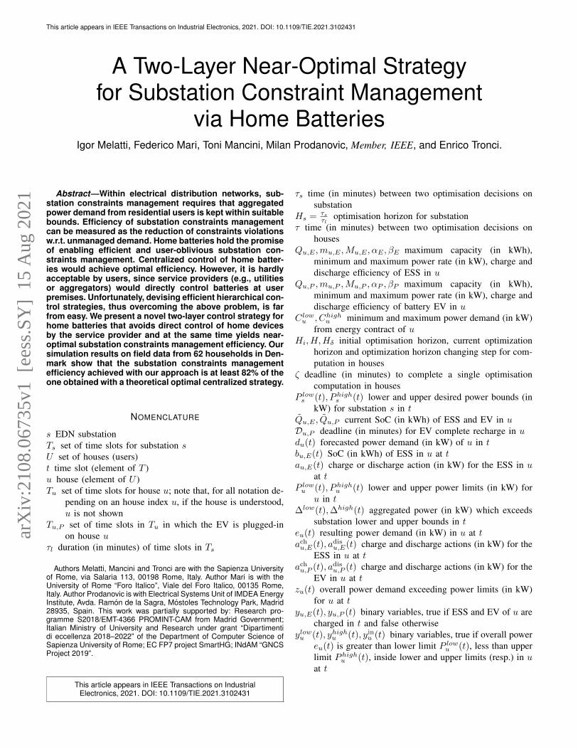
ADAPT Base Algorithm. Both ADAPT and LAHEMSalgorithms are based on the MPC methodology. As for thesystem model (e.g., batteries and power demand) as well asfor the underlining MPC scheme, we follow well-establishedapproaches from the literature, e.g., [2], [10]. Every τs min-utes, the ADAPT algorithm computes the power limits for

This article appears in IEEE Transactions on Industrial Electronics, 2021. DOI: 10.1109/TIE.2021.3102431

Every hour, collect power demands of all houses in U

Compute power demand forecast for the next dayfor each house in U

Create LP L1 and solve itwith an LP solver

Extract from the solution of L1 the power bounds foreach house in U, and sendto each house the corresponding bounds

At midnight of a new day

Read the current power demand and the SOCof battery an EV

Compute power demand forecast for the next H hours

Create LP L2 and solve itwith a MILP solver

Extract from the solution of L2 the actions for thebattery and the EV, andsend such actions to them

If new power bounds areavailable from ADAPT,read and store them

Wait 5 minutes

If one of horizons H-Hd orH+Hd is better than H, replace H with the best one

Fig. 3: Simplified control-flow diagram for ADAPT (left) andLAHEMS (right), also showing the main variables used

all houses u ∈ U . To this aim, a Linear Programming (LP)problem L1 (designed by suitably extending [2]) with recedinghorizon Hs for layer 1 is generated and solved. Namely,L1 contains 6|U ||Ts| + 3|Ts| + |U | constraints, defined over4|U ||Ts|+|U |+2|Ts| real-valued variables, which are detailedin the following.

∀u ∈ U, t ∈ Ts. bu,E(t+ 1) = bu,E(t) +τl60au,E(t) (1)

Constraint (1) states that the SoC bu,E(t + 1) (in kWh) ofthe battery in house u at a given time slot t+1 is the result ofapplying action au,E(t) (in kW) to SoC bu,E(t) at the previoustime slot t, also considering time slot duration in minutes τl.

∀u ∈ U. bu,E(t1) = bu,E(t|Ts| + 1) =Qu,E

2(2)

Constraint (2) states that the behavior of the battery must becyclic, i.e., the starting and ending SoC of the battery (withintime slots set Ts, which lasts one day in our experiments) ina given house u must be both half of the battery maximumcapacity Qu,E . In this way, there are no preferences amongdifferent executions of ADAPT in different days.

∀u ∈ U, t ∈ Ts. P lowu (t) ≤ au,E(t) + du(t) ≤ Phighu (t) (3)

Constraint (3) states that the collaborative power profile foreach u ∈ U must always be inside the bounds P lowu , Phighu

to be output for user u. Note that, following the nomencla-ture in [2], “collaborative power profile” does not refer tocollaborations between users, but to the fact that each useris willing to follow the price policies decided by DSO usingADAPT. Namely, such collaborative power profile is definedby applying an action on the battery au,E(t) to the currentdemand du(t), thus obtaining au,E(t) + du(t).

∀u ∈ U, t ∈ Ts. 0 ≤ bu,E(t) ≤ Qu,E (4)

∀u ∈ U, t ∈ Ts. mu,E ≤ au,E(t) ≤Mu,E (5)

Constraints (4) and (5) require that the power demand shiftau,E for user u is within the limits of user u flexibility, i.e.,within the power rate and capacity of the battery in house u(also Constraint (1) is involved, as it defines the future SoC).

∀u ∈ U, t ∈ Ts. Clowu ≤ P lowu (t) ≤ Phighu (t) ≤ Chighu (6)

Constraint (6) requires that the output bounds P lowu , Phighu

for user u must be within the electricity contract of u.

∀t ∈ Ts. ∆high(t) ≥ 0,∆low(t) ≥ 0 (7)

∀t ∈ Ts.∑u∈U

Phighu (t) ≤ Phighs (t) + ∆high(t) (8)

∀t ∈ Ts.∑u∈U

P lowu (t) ≥ P lows (t)−∆low(t) (9)

Constraints (7)–(9) define the worst-case aggregated powers∆high exceeding Phighs and ∆low going below P lows . Theobjective function of L1 is to minimize all such aggregatedpower exceeding substation bounds, i.e.,

∑t∈Ts

∆high(t) +∑t∈Ts

∆low(t).Finally, every τs minutes, the ADAPT output values for

power limits P lowu (t), Phighu (t), for all u ∈ U, t ∈ Ts, arecomputed by solving, every τs minutes, the LP problemL1 via a LP solver and then extracting, from the obtainedsolution, the values for decision variables P lowu (t), Phighu (t)(the corresponding control-flow diagram is shown in the leftpart of Figure 3).

LAHEMS Base Algorithm. In each house u ∈ U ,every τ minutes, the main LAHEMS algorithm computescharge/discharge decisions on battery and/or EV, basing onthe battery and/or EV current SoC, on the current householdpower demand, on forecasted future power demand, and onthe known future power limits P lowu , Phighu from ADAPT. Inorder to compute the charge/discharge commands, a Mixed In-teger Linear Programming (MILP) problem L2 with recedinghorizon H for layer 2 is generated and solved. L2 consists oftwo separate sets L2E , L2P of constraints. Constraints in L2E

deal with fixed battery dynamics and thus are always present.Constraints in L2P are defined only when the EV is plugged-in. We have that L2E is defined by 22H + 2 constraints on5H+ 1 continuous decision variables and 4H binary decisionvariables. On the other hand, L2P is defined by at most 6H+2constraints on at most 3H continuous decision variables andH binary decision variables, depending on |TP |, being TP thesubset of time slots in T in which the EV will stay plugged-in.In the following, we describe such constraints in more detail.We recall that we focus on a given house u ∈ U , thus we willassume index u to be understood.

∀t ∈ T.e(t)=d(t)+achE (t)−βEadisE (t)+η(t)(achP (t)−βPadisP (t))(10)

∀t ∈ T. Clow ≤ e(t) ≤ Chigh (11)

Constraint (10) defines the power e(t) requested or gener-ated by the house in time slot t ∈ T as the sum of all housespower consumption (power demand d(t), charge commandsfor battery and EV achE (t), achP (t)) and power production(discharge commands for battery and EV adisE (t), adisP (t)). Allsuch values are in kW. Battery and EV discharge commandsalso take into account round-trip inefficiencies 0 < βE , βP <1. Constant η(t) is defined, for a given time slot t, as thefraction of t in which the EV is plugged-in. Constraint (11)requires such resulting power demand e(t) to be inside theranges of the household electricity contract.

bE(t1) = QE , 0 ≤ bE(tH + 1) ≤ QE (12)∀t ∈ T. bE(t+ 1) = bE(t) +

|t|60

(αEachE (t)− adisE (t)) (13)

∀t ∈ T. yE(t)→ achE (t) = 0,¬yE(t)→ adisE (t) = 0 (14)

∀t ∈ T. 0 ≤ bE(t) ≤ QE , 0 ≤ achE (t) ≤ME , 0 ≤ adisE (t) ≤ mE

(15)

This article appears in IEEE Transactions on Industrial Electronics, 2021. DOI: 10.1109/TIE.2021.3102431

Constraints (12) and (13) define the behavior of the battery,i.e., the starting SoC QE (in kWh) is read from sensors, andthe SoC at time t+1 is obtained by adding to the SoC at timet the action taken at time slot t, multiplied by the time slot du-ration |t|. In case of a charge action, the efficiency coefficient0 < αE < 1 is also considered. Constraint (14) allows us todistinguish between a charge and a discharge action, whichis required to apply the known battery efficiencies αE , βE .Furthermore, the battery physical constraints on power rateand capacity are taken into account by Constraint (15). Notethat the Constraints (14) are guarded constraints of the formγ → L(X ) ≤ K or ¬γ → L(X ) ≤ K, where L is a linearfunction, X is a set of bounded variables (i.e., all variables inX are defined on a suitable bounded interval), γ is a binaryvariable not in X and K is a constant. Since all our decisionvariables are bounded, such constraints are translated intolinear constraints as follows: γ → L(X ) ≤ K is equivalentto (sup(L(X )) − K)γ + L(X ) ≤ sup(L(X )), while ¬γ →L(X ) ≤ K is equivalent to (K− sup(L(X )))γ+L(X ) ≤ K.In such formulas, sup(L(X )) may be easily computed as Lis linear and all variables in X are bounded [2].

bP (t1) = QP (16)

∀t ∈ TP . bP (t+ 1) = bP (t) + η(t)|t|60

(αPachP (t)− adisP (t))

(17)∀t ∈ TP . yP (t)→ achP (t) = 0,¬yP (t)→ adisP (t) = 0 (18)

∀t ∈ TP . 0 ≤ bP (t) ≤ QP , 0 ≤ achP (t) ≤MP , 0 ≤ adisP (t) ≤ mP

(19)Constraints (16)–(19) define the analogous behavior for

the EV. Note that such constraints are defined on the setTP = {t1, . . . , t} of the time slots in which the EV is actuallyplugged-in. This implies that Constraints (16)–(19) are onlypresent when the EV is currently plugged-in, thus they are inL2,P . Note that the Constraints (18) are guarded constraints(see above).

bP (t+ 1) = min{QP , QP + αPMPDP }min

{1,

∑t∈T |t|DP

}(20)

To define the goal for EV recharging, we have to considertwo aspects, both handled by Constraint (20) in L2,P . On theone hand, the input deadline specified by the user for the EVcomplete recharge may be infeasible w.r.t. the current SoC(e.g., it is infeasible to completely recharge the EV from 0kWh in 1 hour). In order to avoid L2 to turn out infeasible onlybecause of this, LAHEMS first computes the SoC attainablewith the currently specified deadline, i.e., QP + αPMPDP .On the other hand, the EV may be expected to be unpluggedat time slot t within the current time horizon, or in a time slotthat will be considered in a future MILP. In the former case,the EV must be completely charged at t. In the latter case, werequire the final charge of the EV to be proportional to theremaining time before unplugging the EV, i.e.,

∑t∈T |t|DP

.

∀t ∈ T. yhigh(t)→ e(t) ≤ Phigh(t) (21)

∀t ∈ T. ¬yhigh(t)→ e(t) ≥ Phigh(t) (22)

∀t ∈ T. ylow(t)→ e(t) ≥ P low(t) (23)

∀t ∈ T. ¬ylow(t)→ e(t) ≤ P low(t) (24)

∀t ∈ T. yin(t)→ yhigh(t) + ylow(t) ≥ 2 (25)

∀t ∈ T. ¬yin(t)→ yhigh(t) + ylow(t) ≤ 1 (26)

∀t ∈ T. yin(t)→ z(t) = 0 (27)

∀t ∈ T. ¬yhigh(t)→ z(t) = e(t)− Phigh(t) (28)

∀t ∈ T. ¬ylow(t)→ z(t) = −e(t) + P low(t) (29)∀t ∈ T. 0 ≤ z(t) ≤ max{P low(t)−Clow, Chigh − Phigh(t)}

(30)The objective function of L2 minimizes the power outside

the limits decided by ADAPT for the given house. To thisaim, such exceeding power in time slot t ∈ T is modeled byvariable z(t) (having bounds as in Constraint (30)), thus theobjective function to be minimized is

∑t∈T z(t). By using

guarded constraints (see above), the decision variables z(t)are defined by:• Constraints (21) and (22), where binary variable yhigh(t)

is set to true iff the resulting power e(t) exceeds the upperbound Phigh(t);

• Constraints (23) and (24), where binary variable ylow(t)is set to true iff the resulting power e(t) is below thelower bound P low(t);

• Constraints (25) and (26), where binary variable yin(t)is set to true iff the resulting power e(t) is inside thebounds interval [P low(t), Phigh(t)];

• Constraints (27)–(29), where, exploiting the binary vari-ables defined in Constraints (21)–(26), the real variablez(t) is defined to be 0 iff e(t) ∈ [P low(t), Phigh(t)],and to be the power outside the bounds interval[P low(t), Phigh(t)] otherwise.

Finally, every τ minutes, the LAHEMS output values forbattery and/or EV charging/discharging actions are computedby solving the MILP problem L2 via a MILP solver andthen extracting, from the obtained solution, the actions forthe first time slot in T . If L is infeasible, then a de-fault action is selected, which is designed to minimize userdiscomfort. That is, if the EV is not currently plugged-in or is already fully charged, then no action is taken,i.e., (aE , aP ) = (0, 0). Otherwise, the EV is charged asmuch as possible, also discharging the battery as muchas possible, i.e., aP = min{MP ,

QP−QP

τ , Chigh − d(t1)+

βE min{mE ,QE−QE

τ }}, aE = −min{mE ,QE−QE

τ , aPβE}. In-

stead, if L is feasible, then, for x ∈ {E,P}, ax = achx (t1) ifachx (t1) ≥ 0, and ax = adisx (t1) otherwise. The correspondingcontrol-flow diagram is shown in the right part of Figure 3.

LAHEMS Adaptive Algorithm. Our adaptive algorithm isbased on the fact that using a high value for the horizon H doesnot imply that we obtain better exceeding power minimization.This is due to: i) uncertainties stemming from power demandforecasting, which are worse for higher values of the horizon,and ii) higher computation time typically required to solveMILPs with higher horizons, as the number of both constraintsand decision variables linearly depends on H . Thus, our adap-tive algorithm works as follows. Instead of setting up only oneMILP L with fixed receding horizon H , as it is done in theliterature, LAHEMS sets up and separately solves 3 differentMILPs with receding horizon h ∈ {H,H − Hδ, H + Hδ}

This article appears in IEEE Transactions on Industrial Electronics, 2021. DOI: 10.1109/TIE.2021.3102431

Distributions transformerno. 30378 feeder 1

Distributions transformerno. 30378 feeder 1

L: 85 m4 x 150 AL

L: 23m4 x 95 AL

L: 23m4 x 95 AL

L: 39 m4 x 150 AL

L: 39 m4x150AL

L: 102 m4 x 150 AL

L: 39 m4 x 95 AL

L: 25 m4 x 95 AL

L: 20 m4 x 95 AL

L: 45 m4 x 150 AL

L: 16 m4 x 150 AL

L: 42 m4 x 150 AL

L: 28 m

4x150AL

L: 33 m4x150AL

L: 63 m4 x 95 AL

L: 41 m4 x 95 AL

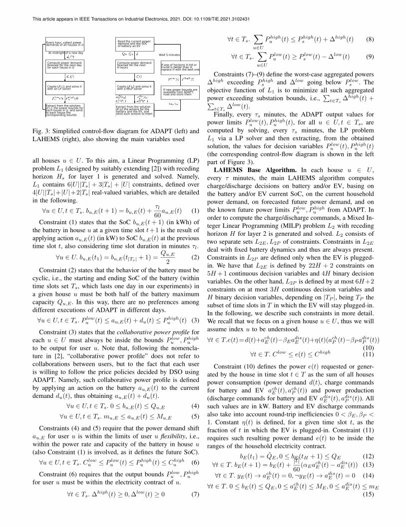
Fig. 4: Net topology of the substation and connected houses

respectively. For each of such MILPs, LAHEMS maintainsthe current objective function value c(h) (i.e., by accumulatingthe values of the MILP objective functions as computed by theMILP solver). When, for some h 6= H , the value for h is betterthan the value for the current horizon H , i.e., c(h) < c(H), thecurrent horizon H is updated to h and all objective functionvalues c(h) are reset to 0. Note that only the actions computedwith the current horizon H (which are computed first) aresent to batteries actuators. Namely, MILP problems with otherhorizons are only used to automatically adjust the currenthorizon, so that the exceeding power is further minimized.

In order to meet real-time requirements, LAHEMS uses atwofold strategy. First of all, LAHEMS stops MILP solverexecution if it exceeds ζ minutes. In this case, the currentMILP problem L is handled as if it were infeasible (i.e.,minimizing user discomfort). This entails that battery actionsare held for τ − ζ minutes. Since, for small values of ζ,τ − ζ ≈ τ , this is in agreement with MILP constraints whichassume computed actions for battery and EV to be held for allcurrent time slot duration τ . Second, after having computed theactions for battery and EV, LAHEMS would be idle till theend of the current time slot duration τ (neglecting periodictasks such as downloading new power limits or reading thecurrent power demand). LAHEMS exploits such although idletime to compute the actions with horizons H −Hδ, H +Hδ ,thus achieving horizon adjustment without overhead.

IV. EXPERIMENTAL SETUP

In this section, we describe how we organize our exper-iments, in order to show the feasibility of our approach. Tothis aim, we implemented both the ADAPT and the LAHEMSalgorithm by using the Python language, and we use GNU Lin-ear Programming Kit (GLPK) to solve MILP problems. Thefollowing results have been obtained by simulating ADAPToperation for one year on an Intel i7 2.5 GHz with 8GBof RAM, and by simulating LAHEMS operation for thesame period, also considering output from ADAPT, on aRaspberry Pi Model B+ 700 MHz with 512 MB of RAM.Our experiments are organized as follows.

Key Performance Indicators. In order to evaluate ourDANCA methodology, we define a set of meaningful KeyPerformance Indicators (KPIs), which are listed and explainedin Table I.

0

0.2

0.4

0.6

0.8

1

1.2

1.4

-5 0 5 10 15 20 25 30 35 40 45 50 55 60 65

Pow

er d

eman

d fr

actio

n

Houses

Day hours in 0-6Day hours in 6-12

Day hours in 12-18Day hours in 18-24

Fig. 5: Houses historical demand distribution

Substation, households and EVs. In order to accuratelysimulate ADAPT and LAHEMS operation for a long enoughperiod, we need power demand data, taken at intervals of atleast one hour, of each residential house connected to a givensubstation. To this aim, we use power demand recorded, fromthe beginning of September 2013 to the end of August 2014,in 62 households in a suburban area in Denmark. All suchhouses are connected to the same substation s (see Figure 4).Such data were recorded during the European Commissionproject “SmartHG” [37], [30] and consists, for each of the 62houses, in the power demand recorded from house electricitymain, with a resolution of 1 hour. We point out that Danishhouseholds use district heating for house heating and elec-tricity for house appliances. We also use Photovoltaic Panel(PVP) energy production recorded in the same period and area.Such recorded data consider 6 kWp PVP installations, withhighly seasonal productivity ranging from 200 kWh/month inDecember and above 1200 kWh/month from April to July.To assess the validity of our case study, we show that, withhigh probability, any operational scenario will be very closeto one of those entailed by the houses U considered in ourcase study. To this end, we divide each day into 4 timeslots t1, . . . , t4 of 6 hours each, with ti = [6(i − 1), 6i)(i = 1, . . . , 4). Let Du(ti) be the total electricity demand (fora whole year, in our case study) of house u within time slot ti,let Dtot

u =∑4i=1Du(ti) be the total (whole year) demand of

house u and let Du(ti) be the fraction of the demand of houseu within time slot ti, i.e., Du(ti) = Du(ti)

Dtotu

. On such a base,we define the demand distribution Du for house u as Du =(Du(t1), Du(t2), Du(t3), Du(t4)

). Figure 5 shows the set of

demand distributions D = {Du | u ∈ U}. Our goal is to showthat any reasonable demand distribution will not be too differ-ent from one of those in D. Accordingly, our set of admissibledemand distributions is D∗ = {(p1, p2, p3, p4) | (∧4

i=1pi ∈[0.1, 0.3]) ∧ (

∑4i=1 pi = 1)}. Given a demand profile p =

(p1, p2, p3, p4) ∈ D∗, we define the distance rmse(p) ofp from D as the minimum root mean square error, i.e.,

rmse(p) = 12 min

{√∑4i=1(pi − Du(ti))2 | u ∈ U

}. Note

that rmse(p) = 0 for p ∈ D. Using MonteCarlo-basedstatistical model checking techniques (e.g., as in [4]), wecan show that, with probability at least 0.99, for a randomlyselected p ∈ D∗ we have rmse(p) ≤ 0.08. That is, with high

This article appears in IEEE Transactions on Industrial Electronics, 2021. DOI: 10.1109/TIE.2021.3102431

TABLE I: List of KPIs used for DANCA evaluation

KPI Description

AvgSolTime Average MILP Solving Time (in seconds), i.e., the average delay due to MILPs solution computationMissDeadl Missed Deadline for MILP Solving, i.e., the fraction of MILPs not solved within the ζ = 0.5 mins deadlineHorChange Horizon Changes. For user u, given N(u) (number of times the adaptive algorithm decided to change the MPC receding

horizon) and T (u) (total number of MILPs), then HorChange = N(u)/T (u)UserDiscomfort Missed EV Deadlines. For user u, given R(u) (number of times the EV was plugged) and M(u) (number of times LAHEMS

failed to fully re-charge the EV within the deadline), then UserDiscomfort = M(u)/R(u)DemOutRed DANCA (Hierarchical) Aggregated Demand Outside Bounds Reduction w.r.t. Historical Demand, i.e., DemOutRed

= 1− ∆(e)∆(d)

(see Section II).DemOutRedOpt Optimal (Centralised) Aggregated Demand Outside Bounds Reduction w.r.t. Historical Demand. Let ∆(c) be the overall

aggregated ADAPT collaborative profile (see Section III) power outside the desired substation bounds. Then, DemOutRedOpt= 1− ∆(c)

∆(d).

TABLE II: Parameters for DANCA evaluation

Param Value Explanation|U | 62 Number of housesτs 1 day Gap between two MILP solver invocations for

ADAPTτl 1 hour Duration of time slots for power limits output

by ADAPTτ 5 min Gap between two MILP solver invocations for

LAHEMSζ 30 sec Deadline for each MILP solver invocation in

LAHEMSHi 6 Starting value for receding horizon in LA-

HEMSHδ 7 Changing step for receding horizon in LA-

HEMSQE 13.5 kWh Battery capacity on each houseME ,mE 3.3 kW Battery power rateα1, β1 0.9 Battery round-trip efficienciesQP 16 kWh EV capacity on each houseMP ,mP 3.6 kW EV power rateα2, β2 0.876 EV round-trip efficiencies

probability, any admissible demand distribution will be veryclose to one of those considered in our case study. This showsthat conclusions drawn from our case study can be safelygeneralized to other situations.

Furthermore, we virtually equip each house with EVscharging data taken from the “Test-an-EV” project [37]. Suchdata consists in plug-in time, SoC at plug-in time and unplugtime for 184 EVs Mitsubishi i-MiEV, ranging from 2012 to2013. The matching between a house and an EV has beendone randomly. We remark that, in ADAPT experiments, EVscharging data is considered a further load for each house u,thus the power demand in a time slot t is incremented by thehistorical charging data of the EV connected to u. In LAHEMSexperiments, we only take into account the starting time andstarting SoC of each recharge, as well as its unplug time.Then, it is LAHEMS responsibility to decide charge/dischargeactions for the EV.

Substation Bounds. We split our experiments into 3 sce-narios, each corresponding to different values for the desiredbounds on substation s required in input by ADAPT. In orderto set up challenging scenarios for our DANCA methodol-ogy, we compute, from the historical data on houses powerconsumption described above (also considering EV rechargingdata), the daily average A(D) and daily maximum M(D) onthe aggregated power demand, being D a given day. A scenarioS is defined by setting, for each day D and all time slots tof D, [P lows (t), Phighs (t)] = [0, A(D) + S(M(D) − A(D))].

That is, we set the lower bound to be 0, as reverse powerflows may damage any installed electrical equipment in thegrid [3]. Instead, for the upper bound, we have that for S = 0 itcoincides with the daily average, whilst for S = 1 it coincideswith the daily maximum. The lower S, the more challengingour scenario is. In the following, we will consider 3 values forS, each defining a scenario, i.e., S ∈ {0, 0.25, 0.5}.

All other experimental parameters are shown in Table II.Simulation of ADAPT in a given day D is carried out bytaking as input the historical data on power demand of allhouses u ∈ U in day D−1, as well as the substation bounds forday D as discussed above. For each house u ∈ U , simulationof LAHEMS in time slot t is carried out by taking as inputthe power limits output by ADAPT for u in Ts, the powerdemand of u in t from historical data, and the estimated SoCof battery and EV in t. Such SoC is computed from the SoCand the charge/discharge action of the previous time slot t−1,using the first time slot of (13) and (17).

V. EXPERIMENTAL RESULTS

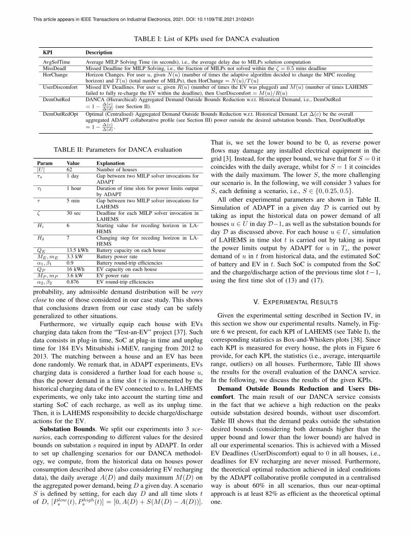
Given the experimental setting described in Section IV, inthis section we show our experimental results. Namely, in Fig-ure 6 we present, for each KPI of LAHEMS (see Table I), thecorresponding statistics as Box-and-Whiskers plots [38]. Sinceeach KPI is measured for every house, the plots in Figure 6provide, for each KPI, the statistics (i.e., average, interquartilerange, outliers) on all houses. Furthermore, Table III showsthe results for the overall evaluation of the DANCA service.In the following, we discuss the results of the given KPIs.

Demand Outside Bounds Reduction and Users Dis-comfort. The main result of our DANCA service consistsin the fact that we achieve a high reduction on the peaksoutside substation desired bounds, without user discomfort.Table III shows that the demand peaks outside the substationdesired bounds (considering both demands higher than theupper bound and lower than the lower bound) are halved inall our experimental scenarios. This is achieved with a MissedEV Deadlines (UserDiscomfort) equal to 0 in all houses, i.e.,deadlines for EV recharging are never missed. Furthermore,the theoretical optimal reduction achieved in ideal conditionsby the ADAPT collaborative profile computed in a centralisedway is about 60% in all scenarios, thus our near-optimalapproach is at least 82% as efficient as the theoretical optimalone.

This article appears in IEEE Transactions on Industrial Electronics, 2021. DOI: 10.1109/TIE.2021.3102431

(a) Average MILP Solving Time (b) Missed Deadline for MILP Solving (c) Horizon Changes

Fig. 6: Box-and-Whisker plots [38] for the main KPIs of LAHEMS. In each plot, the box boundaries are the farthest pointsthat are not outliers (i.e., that are within 1.5 the interquartile range), the line inside the box is the statistical median, and thecircles are data more than 1.5 times the interquartile range from the end of a box.

We remark that these results have been achieved by usingthe same inexpensive hardware that would have been neededby a non-MPC-based strategy. For the sake of comparison,consider a simple strategy where there is only one layer, con-sisting in a computational service acting on each house. Theinput of such service, call it Simple Demand-Aware NetworkConstraint mAnager (SDANCA), is the same as LAHEMS, butinstead of the power bounds computed by ADAPT, SDANCAis directly fed with the desired substation bounds P lows , Phighs

and the number of houses |U |. Given this, SDANCA firstcomputes the house power bounds as P low

s

|U | ,Phigh

s

|U | . Then,SDANCA computes battery and EV actions in a greedy way,i.e., the battery is charged (within its physical limits) whenthe current demand is below the upper bound Phigh

s

|U | , and dis-charged otherwise. Such a simple strategy, while requiring thesame hardware as DANCA, achieves a reduction of substationconstraint management violation of about 38%, compared to50% obtained with our approach.

Computation Time. We recall that LAHEMS is designedto compute each battery and/or EV action in at most ζ = 30seconds. First of all, we point out that MILP deadlines viola-tions are very few, as shown in Figure 6b. Namely, Figure 6bshows that, for most houses, at most 5% (and 2% on average)of all MILP problems solved require more than 30 seconds tobe solved, thus missing the real-time deadline. Furthermore,also considering statistical outliers, the percentage of misseddeadlines is always below 13% in all houses. On the otherhand, Figure 6a shows that most MILP solver invocations,on average, require much lower computation time than 30seconds. Namely, for most houses, the average of the timesneeded to solve all MILP problems (given there is oneMILP solved every 5 minutes over one year, such average iscomputed on about 105,000 values on each house) turns out tobe between 1 and 3 seconds in all scenarios. Furthermore, alsoconsidering the statistical outliers, for all houses the averageMILP solving time is at most 5 seconds. Such results showthat LAHEMS is indeed a lightweight application as requiredand fully meets the requirements for real-time computation

TABLE III: Results for DANCA evaluation

s DemOutRed DemOutRedOpt DemOutRedDemOutRedOpt

0 0.5 0.61 0.820.25 0.53 0.63 0.830.5 0.48 0.58 0.83

on the target low-resource device (Raspberry Pi). Finally, asfor ADAPT computation time, it typically requires at most1 second, which is negligible w.r.t. ADAPT periodicity (1day). This is not surprising, as the MILP problems definedin ADAPT are actually LP problems (i.e., they do not involvebinary decision variables).

Adaptive Algorithm Effectiveness. In order to show theeffectiveness of the adaptive algorithm employed by LA-HEMS, Figure 6c shows the results for the Horizon Changes(HorChange) KPI (see Table I). Namely, in all scenarios andall houses, there are 4 horizon changes every 1000 MILPsolver invocations on average. This shows that our adaptivealgorithm is effective, as it is able to adapt to very differentconditions, depending on the scenario and the current homebehaviour.

VI. CONCLUSIONS

In this paper, we presented Demand-Aware Network Con-straint mAnager, a two-layer computing service that is ableto enforce aggregated power demand constraints on Elec-trical Distribution Network substations. Demand-Aware Net-work Constraint mAnager is composed of two services,both based on the Model Predictive Control methodology:DemAnD–Aware Power limiT, operating once a day at thesubstation level and at utility premises, and LightweightAdaptive Home Energy Management System (also employinga novel adaptive Model Predictive Control), operating onceevery 5 minutes at user premises on hardware with limitedcomputational resources. More in detail, such services act asa hierarchical controller: DemAnD–Aware Power limiT sets

This article appears in IEEE Transactions on Industrial Electronics, 2021. DOI: 10.1109/TIE.2021.3102431

up the long-term goal for Lightweight Adaptive Home En-ergy Management System, which directly controls local homebatteries via charge/discharge commands to meet such goals.Users privacy is also preserved, as only their overall demand issent to the Distribution System Operator, as it already happenswith home mains, and home batteries are not actuated by theDistribution System Operator.

Using power demands recorded in 62 houses in Denmark bythe EU project SmartHG [30], we experimentally showed thatDemand-Aware Network Constraint mAnager is able to reduceaggregated demand bounds violations w.r.t. the unmanageddemand by about 50% on average (w.r.t. 61% reductionobtained by a theoretical optimal centralized solution). This isachieved while meeting real-time requirements on the availablehardware, both at the substation and at the houses level.

Our Demand-Aware Network Constraint mAnager frame-work currently focuses on satisfying the substation (feeder)power bounds. As future work, we plan to investigate how toextend it to enforce other network-level restrictions, e.g., onpower flow.

REFERENCES

[1] M. Uddin, M. F. Romlie, M. F. Abdullah, S. A. Halim], A. H. A.Bakar], and T. C. Kwang], “A review on peak load shaving strategies,”Renewable and Sustainable Energy Reviews, vol. 82, pp. 3323 – 3332,2018. [Online]. Available: http://www.sciencedirect.com/science/article/pii/S1364032117314272

[2] B. P. Hayes, I. Melatti, T. Mancini, M. Prodanovic, and E. Tronci,“Residential demand management using individualized demand awareprice policies,” IEEE Trans. Smart Grid, vol. 8, no. 3, pp. 1284–1294,2017. [Online]. Available: https://doi.org/10.1109/TSG.2016.2596790

[3] D. Dongol, T. Feldmann, E. Bollin, and M. Schmidt, “A model predictivecontrol based peak shaving application of battery for a household withphotovoltaic system in a rural distribution grid.” Sustainable Energy,Grids and Networks, vol. 16, pp. 1 – 13, 2018.

[4] T. Mancini, F. Mari, I. Melatti, I. Salvo, E. Tronci, J. K. Gruber,B. Hayes, M. Prodanovic, and L. Elmegaard, “Parallel statistical modelchecking for safety verification in smart grids,” in 2018 IEEE In-ternational Conference on Communications, Control, and ComputingTechnologies for Smart Grids (SmartGridComm), 2018, pp. 1–6.

[5] A. Jindal, M. Singh, and N. Kumar, “Consumption-aware data analyticaldemand response scheme for peak load reduction in smart grid,” IEEETransactions on Industrial Electronics, vol. 65, no. 11, pp. 8993–9004,2018.

[6] C. E. Kement, H. Gultekin, and B. Tavli, “A holistic analysis of privacy-aware smart grid demand response,” IEEE Transactions on IndustrialElectronics, vol. 68, no. 8, pp. 7631–7641, 2021.

[7] O. Erdinc, A. Tascikaraoglu, N. G. Paterakis, and J. P. S. Catalao, “Novelincentive mechanism for end-users enrolled in dlc-based demand re-sponse programs within stochastic planning context,” IEEE Transactionson Industrial Electronics, vol. 66, no. 2, pp. 1476–1487, 2019.

[8] D. Zhao, H. Wang, J. Huang, and X. Lin, “Virtual energy storage sharingand capacity allocation,” IEEE Transactions on Smart Grid, vol. 11,no. 2, pp. 1112–1123, 2020.

[9] Y. Du and F. Li, “Intelligent multi-microgrid energy management basedon deep neural network and model-free reinforcement learning,” IEEETransactions on Smart Grid, vol. 11, no. 2, pp. 1066–1076, 2020.

[10] N. Zhang, B. D. Leibowicz, and G. A. Hanasusanto, “Optimal residentialbattery storage operations using robust data-driven dynamic program-ming,” IEEE Transactions on Smart Grid, vol. 11, no. 2, pp. 1771–1780,2020.

[11] B. Zhou, K. Zhang, K. W. Chan, C. Li, X. Lu, S. Bu, and X. Gao,“Optimal coordination of electric vehicles for virtual power plants withdynamic communication spectrum allocation,” IEEE Transactions onIndustrial Informatics, vol. 17, no. 1, pp. 450–462, 2021.

[12] D. A. Chekired, L. Khoukhi, and H. T. Mouftah, “Fog-computing-basedenergy storage in smart grid: A cut-off priority queuing model forplug-in electrified vehicle charging,” IEEE Transactions on IndustrialInformatics, vol. 16, no. 5, pp. 3470–3482, 2020.

[13] D. Setlhaolo, X. Xia, and J. Zhang, “Optimal scheduling ofhousehold appliances for demand response,” Electric Power SystemsResearch, vol. 116, pp. 24–28, 2014. [Online]. Available: https://www.sciencedirect.com/science/article/pii/S0378779614001527

[14] A. Jindal, B. S. Bhambhu, M. Singh, N. Kumar, and K. Naik, “Aheuristic-based appliance scheduling scheme for smart homes,” IEEETransactions on Industrial Informatics, vol. 16, no. 5, pp. 3242–3255,2020.

[15] A. Saad, T. Youssef, A. T. Elsayed, A. Amin, O. H. Abdalla, andO. Mohammed, “Data-centric hierarchical distributed model predictivecontrol for smart grid energy management,” IEEE Transactions onIndustrial Informatics, vol. 15, no. 7, pp. 4086–4098, 2019.

[16] D. Li, W.-Y. Chiu, H. Sun, and H. V. Poor, “Multiobjective optimizationfor demand side management program in smart grid,” IEEE Transactionson Industrial Informatics, vol. 14, no. 4, pp. 1482–1490, 2018.

[17] Y. Chai, L. Guo, C. Wang, Y. Liu, and Z. Zhao, “Hierarchical distributedvoltage optimization method for hv and mv distribution networks,” IEEETransactions on Smart Grid, vol. 11, no. 2, pp. 968–980, March 2020.

[18] X. Wu, Y. Xu, X. Wu, J. He, J. M. Guerrero, C. Liu, K. P. Schneider,and D. T. Ton, “A two-layer distributed cooperative control method forislanded networked microgrid systems,” IEEE Transactions on SmartGrid, vol. 11, no. 2, pp. 942–957, 2020.

[19] D. I. Brandao, W. M. Ferreira, A. M. S. Alonso, E. Tedeschi, andF. P. MarafA£o, “Optimal multiobjective control of low-voltage acmicrogrids: Power flow regulation and compensation of reactive powerand unbalance,” IEEE Transactions on Smart Grid, vol. 11, no. 2, pp.1239–1252, 2020.

[20] M. Razmara, G. R. Bharati, M. Shahbakhti, S. Paudyal, and R. D.Robinett, “Bilevel optimization framework for smart building-to-gridsystems,” IEEE Trans. Smart Grid, vol. 9, no. 2, pp. 582–593, 2018.[Online]. Available: https://doi.org/10.1109/TSG.2016.2557334

[21] W. Shi, X. Xie, C. Chu, and R. Gadh, “Distributed optimal energymanagement in microgrids,” IEEE Transactions on Smart Grid, vol. 6,no. 3, pp. 1137–1146, 2015.

[22] D. H. Nguyen, S.-I. Azuma, and T. Sugie, “Novel control approachesfor demand response with real-time pricing using parallel and distributedconsensus-based admm,” IEEE Transactions on Industrial Electronics,vol. 66, no. 10, pp. 7935–7945, 2019.

[23] K. Trangbaek, J. Bendtsen, and J. Stoustrup, “Hierarchical controlfor smart grids,” IFAC Proceedings Volumes, vol. 44, no. 1, pp.6130 – 6135, 2011, 18th IFAC World Congress. [Online]. Available:http://www.sciencedirect.com/science/article/pii/S1474667016445866

[24] P. Paudyal, P. Munankarmi, Z. Ni, and T. M. Hansen, “A hierarchicalcontrol framework with a novel bidding scheme for residential commu-nity energy optimization,” IEEE Transactions on Smart Grid, vol. 11,no. 1, pp. 710–719, 2020.

[25] S. Thangavel, S. Lucia, R. Paulen, and S. Engell, “Dual robustnonlinear model predictive control: A multi-stage approach,” Journalof Process Control, vol. 72, pp. 39 – 51, 2018. [Online]. Available:http://www.sciencedirect.com/science/article/pii/S0959152418304050

[26] M. Guay, V. Adetola, and D. DeHaan, Robust and Adaptive ModelPredictive Control of Nonlinear Systems. Institution of Engineeringand Technology, 2015.

[27] M. Short and F. Abugchem, “A microcontroller-based adaptivemodel predictive control platform for process control applications,”Electronics, vol. 6, no. 4, 2017. [Online]. Available: http://www.mdpi.com/2079-9292/6/4/88

[28] C. Chen, J. Wang, Y. Heo, and S. Kishore, “MPC-based appliancescheduling for residential building energy management controller,” IEEETransactions on Smart Grid, vol. 4, no. 3, pp. 1401–1410, 2013.

[29] S. Lucia, M. J. Kogel, P. Zometa, D. E. Quevedo, and R. Findeisen,“Predictive control, embedded cyberphysical systems and systems ofsystems - A perspective,” Annual Reviews in Control, vol. 41, pp. 193–207, 2016.

[30] V. Alimguzhin, F. Mari, I. Melatti, E. Tronci, E. Ebeid, S. Mikkelsen,R. Hylsberg Jacobsen, J. Gruber, B. Hayes, F. Huerta, and M. Pro-danovic, “A glimpse of smarthg project test-bed and communicationinfrastructure,” in Digital System Design (DSD), 2015 Euromicro Con-ference on, Aug 2015, pp. 225–232.

[31] V. Pop, H. J. Bergveld, D. Danilov, P. P. L. Regtien, and P. H. L. Notten,Battery Management Systems: Accurate State-of-Charge Indication forBattery-Powered Applications. Springer, 2008.

[32] L. He, L. Kong, S. Lin, S. Ying, Y. J. Gu, T. He, and C. Liu, “RAC:reconfiguration-assisted charging in large-scale lithium-ion batterysystems,” IEEE Trans. Smart Grid, vol. 7, no. 3, pp. 1420–1429, 2016.[Online]. Available: https://doi.org/10.1109/TSG.2015.2450727

This article appears in IEEE Transactions on Industrial Electronics, 2021. DOI: 10.1109/TIE.2021.3102431

[33] E. Chemali, P. J. Kollmeyer, M. Preindl, R. Ahmed, and A. Emadi,“Long short-term memory networks for accurate state-of-charge estima-tion of li-ion batteries,” IEEE Transactions on Industrial Electronics,vol. 65, no. 8, pp. 6730–6739, 2018.

[34] K. Li, F. Wei, K. J. Tseng, and B.-H. Soong, “A practical lithium-ion battery model for state of energy and voltage responses predictionincorporating temperature and ageing effects,” IEEE Transactions onIndustrial Electronics, vol. 65, no. 8, pp. 6696–6708, 2018.

[35] C. Yu, P. W. Mirowski, and T. K. Ho, “A sparse coding approach tohousehold electricity demand forecasting in smart grids,” IEEE Trans.Smart Grid, vol. 8, no. 2, pp. 738–748, 2017. [Online]. Available:https://doi.org/10.1109/TSG.2015.2513900

[36] T. Li, Y. Wang, and N. Zhang, “Combining probability density forecastsfor power electrical loads,” IEEE Transactions on Smart Grid, vol. 11,no. 2, pp. 1679–1690, 2020.

[37] European Commision project SmartHG. (2015). [Online]. Available:http://smarthg.di.uniroma1.it/

[38] J. W. Tukey, Exploratory Data Analysis, ser. Behavioral Science: Quan-titative Methods. Reading, Mass.: Addison-Wesley, 1977.

Igor Melatti was born in Treviso, Italy. He re-ceived the Master Degree in Computer Scienceand the PhD in Computer Science and Applica-tions from the University of L’Aquila, Italy in 2001and 2005 respectively. He has been a PostDocat the University of Utah and at the SapienzaUniversity of Rome. He is currently an AssociateProfessor at the Computer Science Departmentof Sapienza University of Rome. His currentresearch interests comprise: formal methods,automatic verification algorithms, model check-

ing, software verification, cyber-physical systems, automatic synthesisof reactive programs from formal specification, systems biology, smartgrids.

Federico Mari was born in Treviso, Italy. Hereceived the Master Degree and the PhD inComputer Science from the Sapienza Universityof Rome, Italy in 2006 and 2010 respectively.He is currently an Assistant Professor (tenuretrack) of Computer Science at the Departmentof Movement, Human and Health Sciences ofthe University of Rome Foro Italico (from 2019),where he serves as Rector’s delegate for ICT.His primary research interest is in formal meth-ods and artificial intelligence applied to smart

grids, health and sport sciences.

Toni Mancini has a Ph.D. in Computer Sci-ence Engineering and is Associate Professor atthe Computer Science Department of SapienzaUniversity of Rome, Rome, Italy. His researchinterests comprise: artificial intelligence, formalverification, cyber-physical systems, control soft-ware synthesis, systems biology, smart grids.

Enrico Tronci is a Full Professor at the Com-puter Science Department of Sapienza Univer-sity of Rome (Italy). He received a master’sdegree in Electrical Engineering from SapienzaUniversity of Rome and a Ph.D. degree in Ap-plied Mathematics from Carnegie Mellon Uni-versity. His research interests comprise: formalverification, model checking, system level formalverification, hybrid systems, embedded systems,cyber-physical systems, control software syn-thesis, smart grids, autonomous demand and

response systems for smart grids, systems biology

Milan Prodanovic (M01) received the B.Sc. de-gree in electrical engineering from the Univer-sity of Belgrade, Serbia, in 1996 and the Ph.D.degree from Imperial College, London, U.K., in2004. From 1997 to 1999 he was engaged withGVS engineering company, Serbia, developingUPS systems. From 1999 until 2010 he was aresearch associate in Electrical and ElectronicEngineering at Imperial College, London, UK.Currently he is a Senior Researcher and Headof the Electrical Systems Unit at Institute IMDEA

Energy, Madrid, Spain. His research interests include design and controlof power electronics interfaces for distributed generation, micro-gridscontrol and active management of distribution networks.

This article appears in IEEE Transactions on IndustrialElectronics, 2021. DOI: 10.1109/TIE.2021.3102431