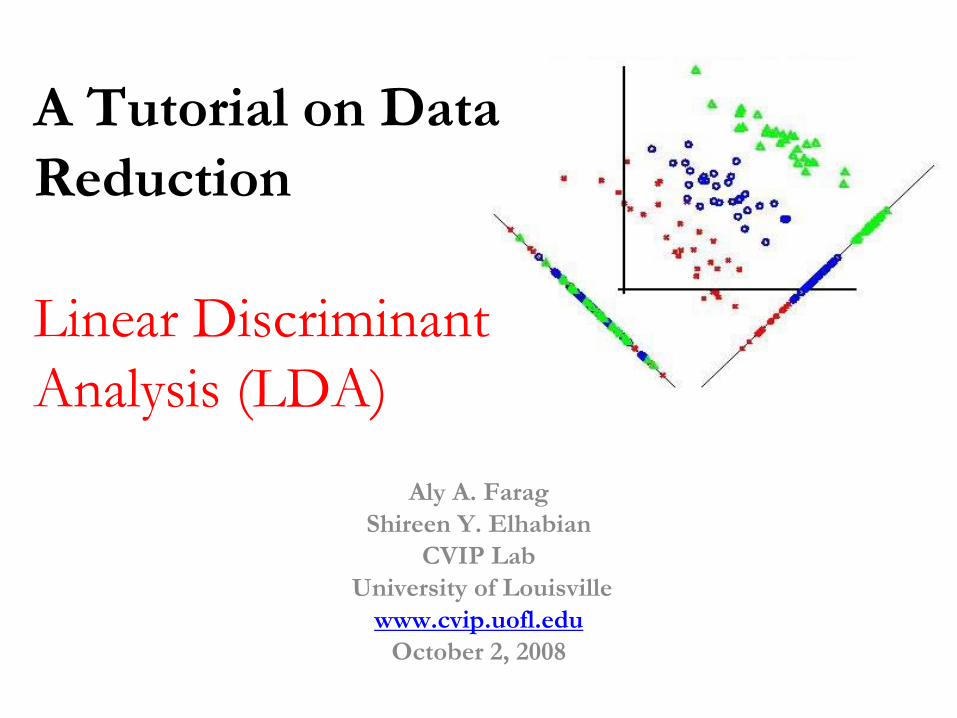
A Tutorial on Data Reduction

Linear Discriminant

Analysis (LDA)Aly A. Farag

Shireen Y. ElhabianCVIP Lab

University of Louisvillewww.cvip.uofl.edu

October 2, 2008

Outline• LDA objective

• Recall …

PCA

• Now …

LDA

• LDA …

Two Classes

– Counter example

• LDA …

C Classes

– Illustrative Example

• LDA vs

PCA Example

• Limitations of LDA

LDA Objective

• The objective of LDA is to perform dimensionality reduction …

– So what, PCA does this …

• However, we want to preserve as much of the class discriminatory information as possible.

– OK, that’s new, let dwell deeper ☺…

Recall …

PCA

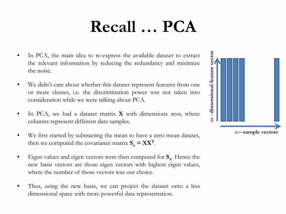
• In PCA, the main idea to re-express the available dataset to extract the relevant information by reducing the redundancy and minimize

the noise.

• We didn’t care about whether this dataset represent features from one or more classes, i.e. the discrimination power was not taken into consideration while we were talking about PCA.

• In PCA, we had a dataset matrix X

with dimensions mxn, where columns represent different data samples.

• We first started by subtracting the mean to have a zero mean dataset, then we computed the covariance matrix Sx

= XXT.

• Eigen

values and eigen

vectors were then computed for Sx

. Hence the new basis vectors are those eigen

vectors with highest eigen

values, where the number of those vectors was our choice.

• Thus, using the new basis, we can project the dataset onto a less dimensional space with more powerful data representation.

n –

sample vectors

m-

dim

ensi

onal

fea

ture

vec

tor

Now …

LDA

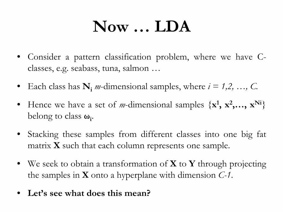
• Consider a pattern classification problem, where we have C- classes, e.g. seabass, tuna, salmon …

• Each class has Ni

m-dimensional samples, where i = 1,2, …, C.

• Hence we have a set of m-dimensional samples {x1, x2,…, xNi} belong to class ωi

.

• Stacking these samples from different classes into one big fat matrix X such that each column represents one sample.

• We seek to obtain a transformation of X

to Y

through projecting the samples in X

onto a hyperplane

with dimension C-1.

• Let’s see what does this mean?

LDA …

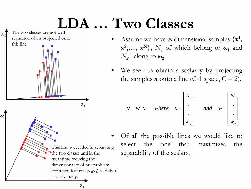
Two Classes• Assume we have m-dimensional samples {x1,

x2,…, xN}, N1

of which belong to ω1

and N2

belong to ω2

.

• We seek to obtain a scalar y by projecting the samples x

onto a line (C-1 space, C = 2).

• Of all the possible lines we would like to select the one that maximizes the separability

of the scalars.

⎥⎥⎥⎥

⎦

⎤

⎢⎢⎢⎢

⎣

⎡

=

⎥⎥⎥⎥

⎦

⎤

⎢⎢⎢⎢

⎣

⎡

==

mm

T

w

w

wand

x

x

xwherexwy..

.

.11

The two classes are not well separated when projected onto this line

This line succeeded in separating the two classes and in the meantime reducing the dimensionality of our problem from two features (x1

,x2

) to only a scalar value y.

LDA …

Two Classes

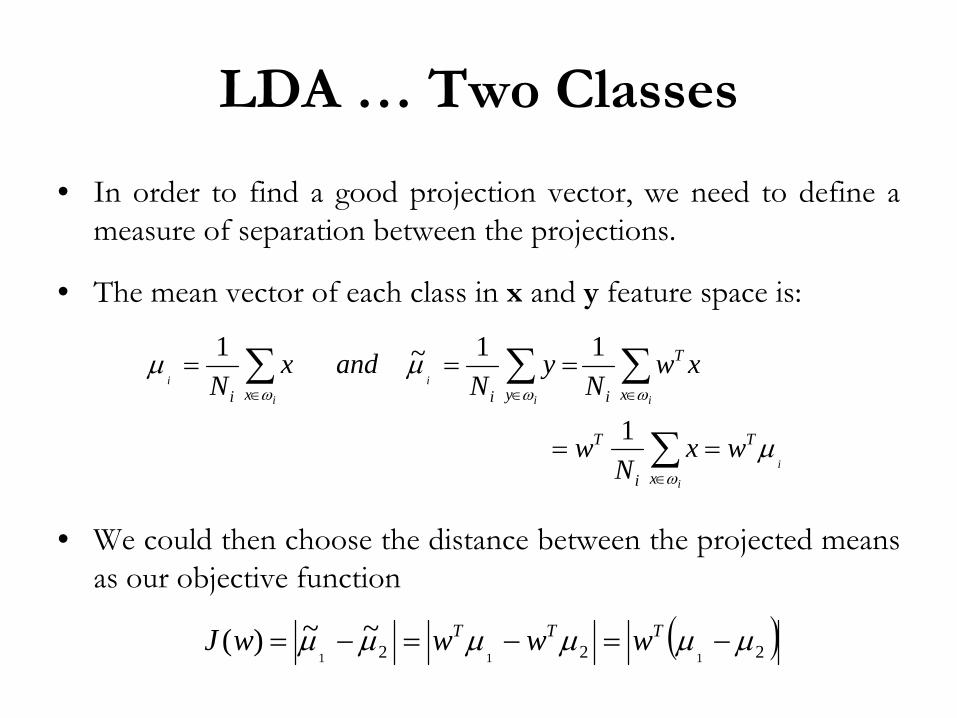
• In order to find a good projection vector, we need to define a measure of separation between the projections.

• The mean vector of each class in x

and y

feature space is:

• We could then choose the distance between the projected means as our objective function

i

i

ii

i

i

i

T

xi

T

x

T

iyixi

wxN

w

xwN

yN

andxN

μ

μμ

ω

ωωω

==

===

∑

∑∑∑

∈

∈∈∈

1

11~1

( )222 111

~~)( μμμμμμ −=−=−= TTT wwwwJ

LDA …

Two Classes

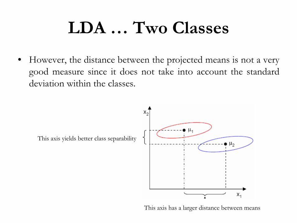
• However, the distance between the projected means is not a very good measure since it does not take into account the standard deviation within the classes.

This axis has a larger distance between means

This axis yields better class separability

LDA …

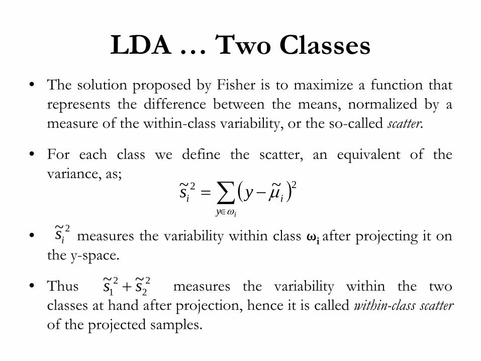
Two Classes• The solution proposed by Fisher is to maximize a function that

represents the difference between the means, normalized by a measure of the within-class variability, or the so-called scatter.

• For each class we define the scatter, an equivalent of the variance, as;

• measures the variability within class ωi after projecting it on the y-space.

• Thus measures the variability within the two classes at hand after projection, hence it is called within-class scatter

of the projected samples.

( )∑∈

−=iy

ii ysω

μ 22 ~~

2~is

22

21

~~ ss +

LDA …

Two Classes

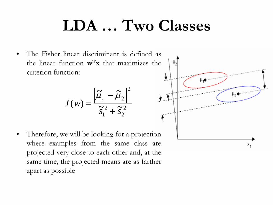
• The Fisher linear discriminant

is defined as the linear function wTx

that maximizes the criterion function:

• Therefore, we will be looking for a projection where examples from the same class are

projected very close to each other and, at the same time, the projected means are as farther apart as possible

22

21

2

2

~~~~

)( 1

sswJ

+

−=

μμ

LDA …

Two Classes

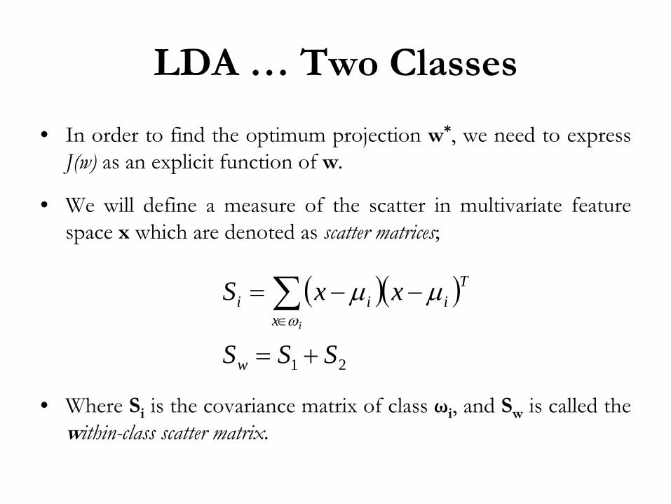
• In order to find the optimum projection w*, we need to express J(w)

as an explicit function of w.

• We will define a measure of the scatter in multivariate feature space x

which are denoted as scatter matrices;

• Where Si

is the covariance matrix of class ωi

, and Sw

is called the within-class scatter matrix.

( )( )

21 SSS

xxS

w

Ti

xii

i

+=

−−= ∑∈

μμω

LDA …

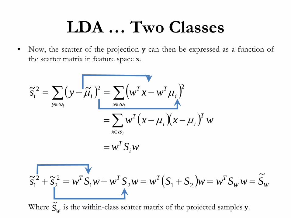
Two Classes• Now, the scatter of the projection y can then be expressed as a function of

the scatter matrix in feature space x.

Where is the within-class scatter matrix of the projected samples y.

( ) ( )

( )( )

( ) WWTTTT

iT

x

Tii

T

xi

TT

yii

SwSwwSSwwSwwSwss

wSw

wxxw

wxwys

i

ii

~~~

~~

21212

22

1

222

==+=+=+

=

−−=

−=−=

∑

∑∑

∈

∈∈

ω

ωω

μμ

μμ

WS~

LDA …

Two Classes

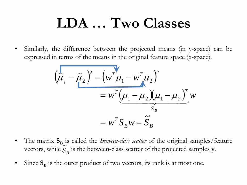
• Similarly, the difference between the projected means (in y-space) can be expressed in terms of the means in the original feature space (x-space).

• The matrix SB

is called the between-class scatter of the original samples/feature vectors, while is the between-class scatter of the projected samples y.

• Since SB

is the outer product of two vectors, its rank is at most one.

( ) ( )( )( )

BBT

S

TT

TT

SwSw

ww

ww

B

~

~~

2121

221

221

==

−−=

−=−

444 3444 21μμμμ

μμμμ

BS~

LDA …

Two Classes

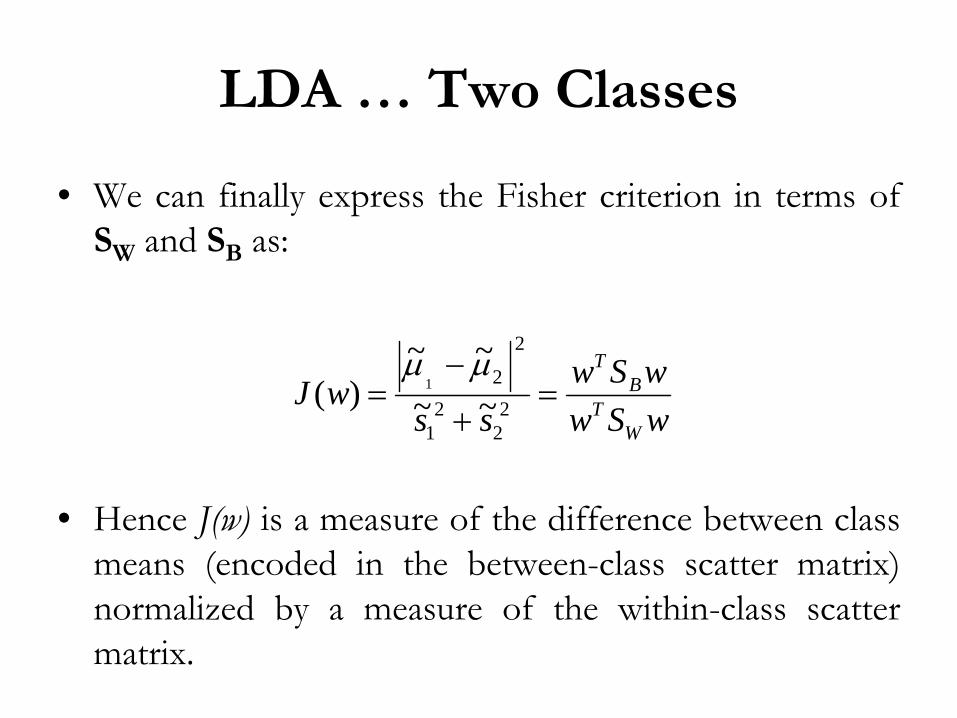
• We can finally express the Fisher criterion in terms of SW

and SB

as:

• Hence J(w)

is a measure of the difference between class means (encoded in the between-class scatter matrix) normalized by a measure of the within-class scatter matrix.

wSwwSw

sswJ

WT

BT

=+

−= 2

22

1

2

2

~~~~

)( 1μμ

LDA …

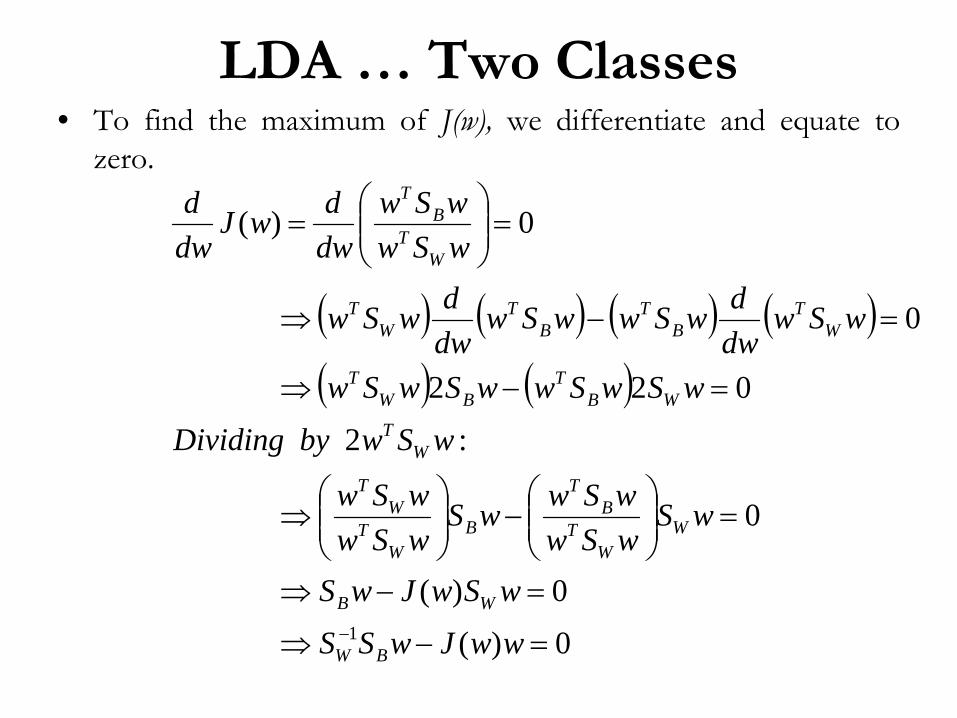
Two Classes• To find the maximum of J(w), we differentiate and equate to

zero.

( ) ( ) ( ) ( )( ) ( )

0)(

0)(

0

:2

022

0

0)(

1 =−⇒

=−⇒

=⎟⎟⎠

⎞⎜⎜⎝

⎛−⎟⎟

⎠

⎞⎜⎜⎝

⎛⇒

=−⇒

=−⇒

=⎟⎟⎠

⎞⎜⎜⎝

⎛=

− wwJwSS

wSwJwS

wSwSwwSwwS

wSwwSw

wSwbyDividing

wSwSwwSwSw

wSwdwdwSwwSw

dwdwSw

wSwwSw

dwdwJ

dwd

BW

WB

WW

TB

T

BW

TW

T

WT

WBT

BWT

WT

BT

BT

WT

WT

BT

LDA …

Two Classes

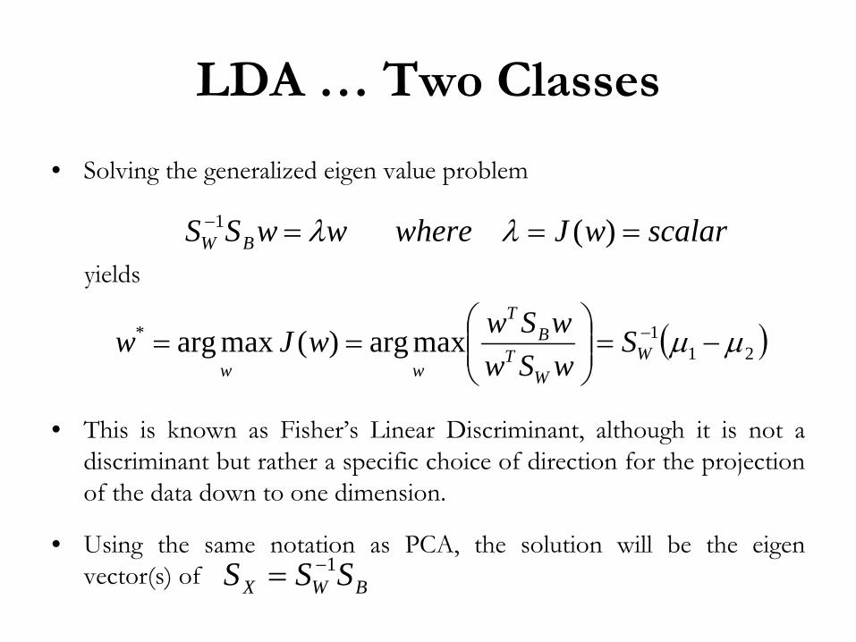
• Solving the generalized eigen

value problem

yields

• This is known as Fisher’s Linear Discriminant, although it is not a discriminant

but rather a specific choice of direction for the projection

of the data down to one dimension.

• Using the same notation as PCA, the solution will be the eigen

vector(s) of

scalarwJwherewwSS BW ===− )(1 λλ

( )211* maxarg)(maxarg μμ −=⎟⎟

⎠

⎞⎜⎜⎝

⎛== −

WW

TB

T

wwS

wSwwSwwJw

BWX SSS 1−=

LDA …

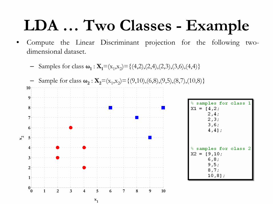
Two Classes -

Example• Compute the Linear Discriminant

projection for the following two-

dimensional dataset.

– Samples for class ω1

: X1

=(x1

,x2

)={(4,2),(2,4),(2,3),(3,6),(4,4)}

– Sample for class ω2

: X2

=(x1

,x2

)={(9,10),(6,8),(9,5),(8,7),(10,8)}

0 1 2 3 4 5 6 7 8 9 100

1

2

3

4

5

6

7

8

9

10

x1

x 2

LDA …

Two Classes -

Example

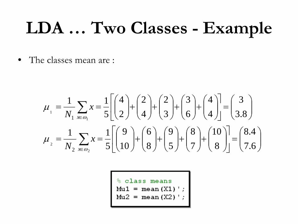
• The classes mean are :

⎟⎟⎠

⎞⎜⎜⎝

⎛=⎥

⎦

⎤⎢⎣

⎡⎟⎟⎠

⎞⎜⎜⎝

⎛+⎟⎟⎠

⎞⎜⎜⎝

⎛+⎟⎟

⎠

⎞⎜⎜⎝

⎛+⎟⎟⎠

⎞⎜⎜⎝

⎛+⎟⎟⎠

⎞⎜⎜⎝

⎛==

⎟⎟⎠

⎞⎜⎜⎝

⎛=⎥

⎦

⎤⎢⎣

⎡⎟⎟⎠

⎞⎜⎜⎝

⎛+⎟⎟⎠

⎞⎜⎜⎝

⎛+⎟⎟⎠

⎞⎜⎜⎝

⎛+⎟⎟⎠

⎞⎜⎜⎝

⎛+⎟⎟

⎠

⎞⎜⎜⎝

⎛==

∑

∑

∈

∈

6.74.8

810

78

59

86

109

511

8.33

44

63

32

42

24

511

2

2

1

1

2

1

ω

ω

μ

μ

x

x

xN

xN

LDA …

Two Classes -

Example

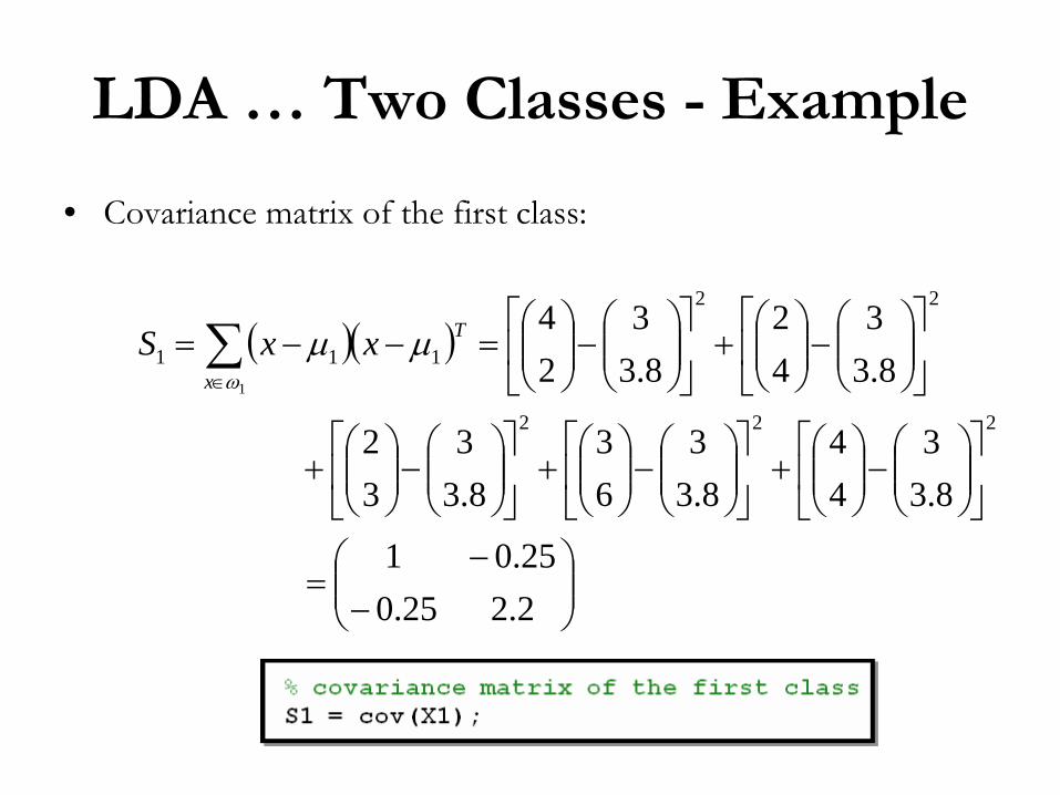
• Covariance matrix of the first class:

( )( )

⎟⎟⎠

⎞⎜⎜⎝

⎛−

−=

⎥⎦

⎤⎢⎣

⎡⎟⎟⎠

⎞⎜⎜⎝

⎛−⎟⎟⎠

⎞⎜⎜⎝

⎛+⎥

⎦

⎤⎢⎣

⎡⎟⎟⎠

⎞⎜⎜⎝

⎛−⎟⎟⎠

⎞⎜⎜⎝

⎛+⎥

⎦

⎤⎢⎣

⎡⎟⎟⎠

⎞⎜⎜⎝

⎛−⎟⎟⎠

⎞⎜⎜⎝

⎛+

⎥⎦

⎤⎢⎣

⎡⎟⎟⎠

⎞⎜⎜⎝

⎛−⎟⎟⎠

⎞⎜⎜⎝

⎛+⎥

⎦

⎤⎢⎣

⎡⎟⎟⎠

⎞⎜⎜⎝

⎛−⎟⎟⎠

⎞⎜⎜⎝

⎛=−−= ∑

∈

2.225.025.01

8.33

44

8.33

63

8.33

32

8.33

42

8.33

24

222

22

1111

T

x

xxS μμω

LDA …

Two Classes -

Example

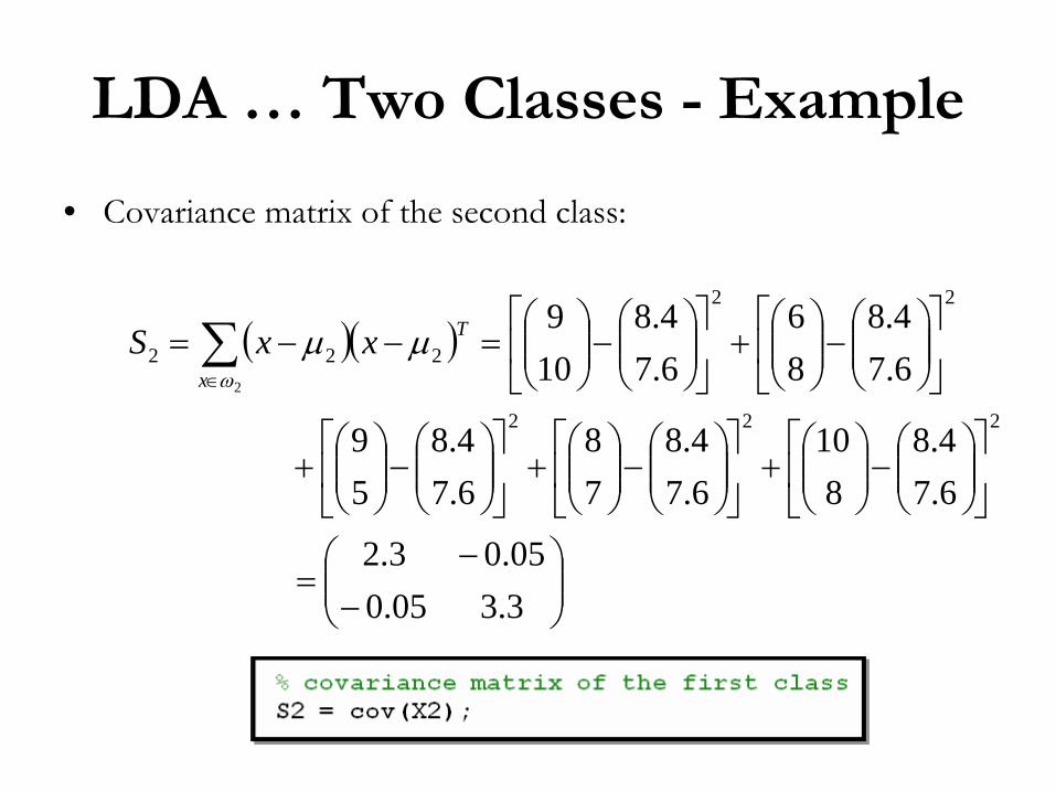
• Covariance matrix of the second class:

( )( )

⎟⎟⎠

⎞⎜⎜⎝

⎛−

−=

⎥⎦

⎤⎢⎣

⎡⎟⎟⎠

⎞⎜⎜⎝

⎛−⎟⎟⎠

⎞⎜⎜⎝

⎛+⎥

⎦

⎤⎢⎣

⎡⎟⎟⎠

⎞⎜⎜⎝

⎛−⎟⎟⎠

⎞⎜⎜⎝

⎛+⎥

⎦

⎤⎢⎣

⎡⎟⎟⎠

⎞⎜⎜⎝

⎛−⎟⎟⎠

⎞⎜⎜⎝

⎛+

⎥⎦

⎤⎢⎣

⎡⎟⎟⎠

⎞⎜⎜⎝

⎛−⎟⎟⎠

⎞⎜⎜⎝

⎛+⎥

⎦

⎤⎢⎣

⎡⎟⎟⎠

⎞⎜⎜⎝

⎛−⎟⎟⎠

⎞⎜⎜⎝

⎛=−−= ∑

∈

3.305.005.03.2

6.74.8

810

6.74.8

78

6.74.8

59

6.74.8

86

6.74.8

109

222

22

2222

T

x

xxS μμω

LDA …

Two Classes -

Example

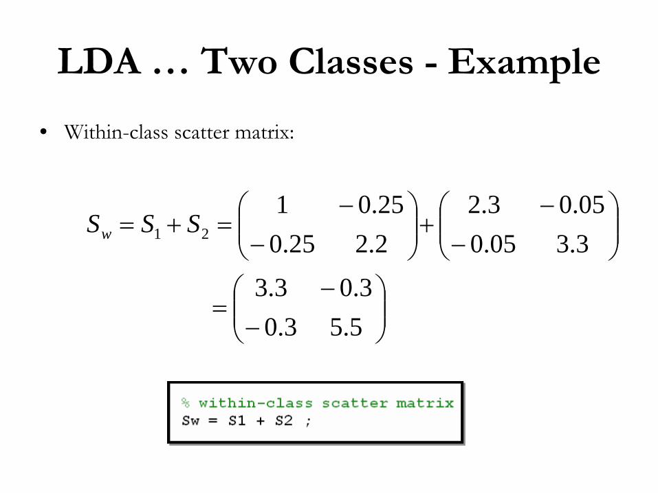
• Within-class scatter matrix:

⎟⎟⎠

⎞⎜⎜⎝

⎛−

−=

⎟⎟⎠

⎞⎜⎜⎝

⎛−

−+⎟⎟⎠

⎞⎜⎜⎝

⎛−

−=+=

5.53.03.03.3

3.305.005.03.2

2.225.025.01

21 SSSw

LDA …

Two Classes -

Example

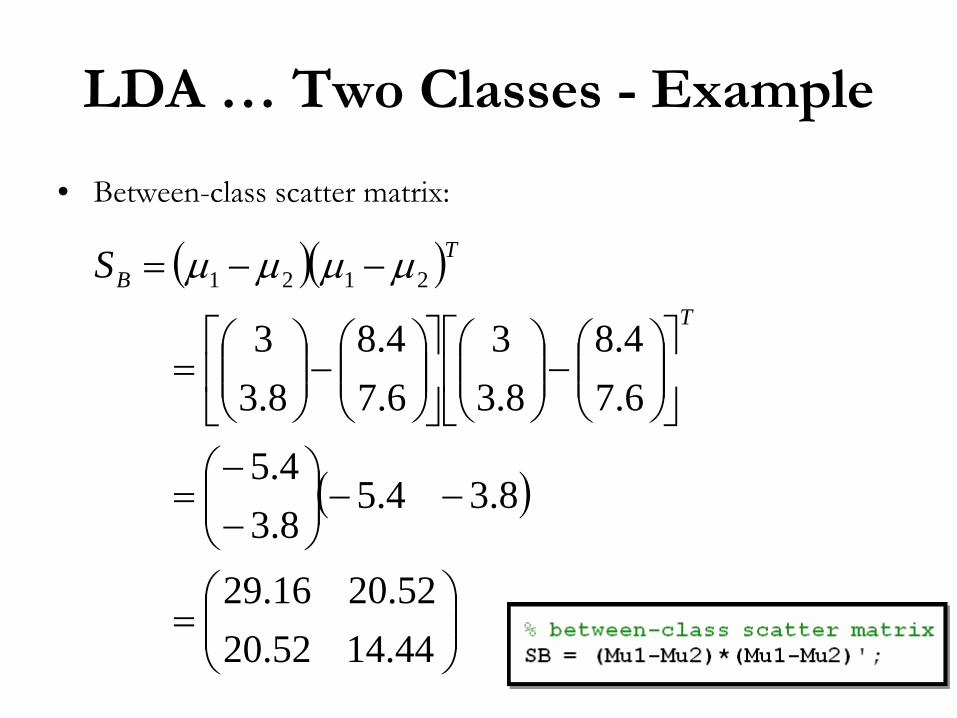
• Between-class scatter matrix:

( )( )

( )

⎟⎟⎠

⎞⎜⎜⎝

⎛=

−−⎟⎟⎠

⎞⎜⎜⎝

⎛−−

=

⎥⎦

⎤⎢⎣

⎡⎟⎟⎠

⎞⎜⎜⎝

⎛−⎟⎟⎠

⎞⎜⎜⎝

⎛⎥⎦

⎤⎢⎣

⎡⎟⎟⎠

⎞⎜⎜⎝

⎛−⎟⎟⎠

⎞⎜⎜⎝

⎛=

−−=

44.1452.2052.2016.29

8.34.58.34.5

6.74.8

8.33

6.74.8

8.33

2121T

TBS μμμμ

LDA …

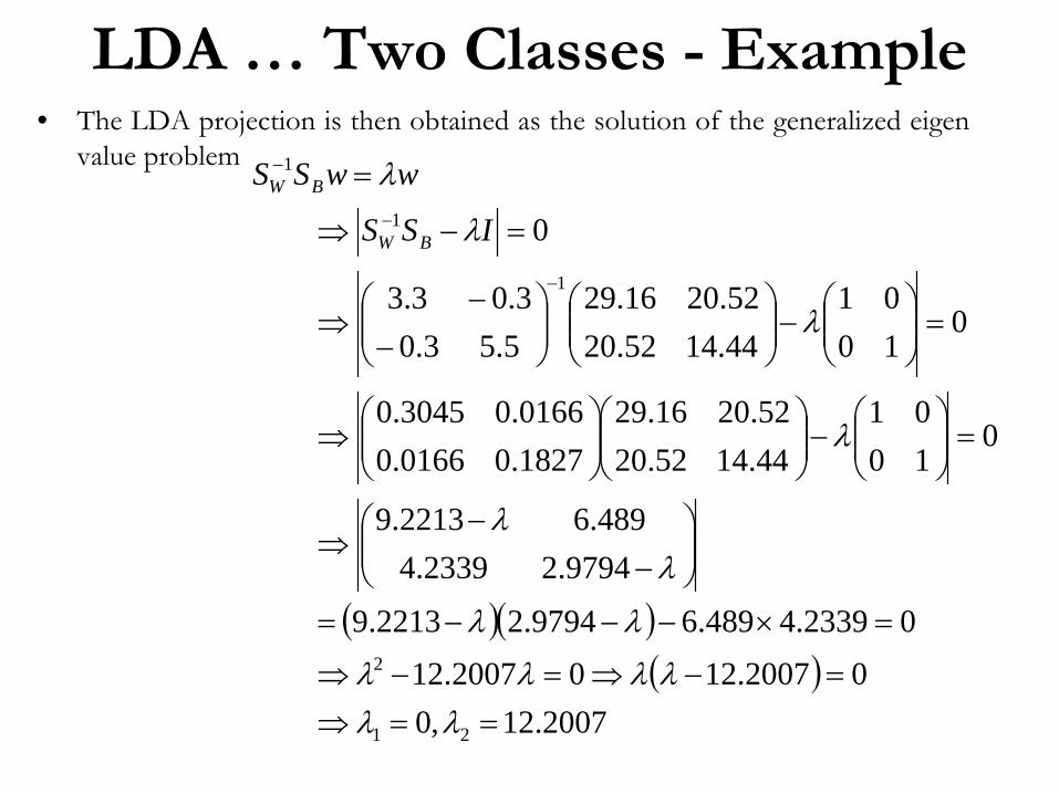
Two Classes -

Example• The LDA projection is then obtained as the solution of the generalized eigen

value problem

( )( )( )

2007.12,002007.1202007.12

02339.4489.69794.22213.9

9794.22339.4489.62213.9

01001

44.1452.2052.2016.29

1827.00166.00166.03045.0

01001

44.1452.2052.2016.29

5.53.03.03.3

0

21

2

1

1

1

==⇒=−⇒=−⇒

=×−−−=

⎟⎟⎠

⎞⎜⎜⎝

⎛−

−⇒

=⎟⎟⎠

⎞⎜⎜⎝

⎛−⎟⎟⎠

⎞⎜⎜⎝

⎛⎟⎟⎠

⎞⎜⎜⎝

⎛⇒

=⎟⎟⎠

⎞⎜⎜⎝

⎛−⎟⎟⎠

⎞⎜⎜⎝

⎛⎟⎟⎠

⎞⎜⎜⎝

⎛−

−⇒

=−⇒

=

−

−

−

λλλλλλ

λλ

λλ

λ

λ

λ

λ

ISS

wwSS

BW

BW

LDA …

Two Classes -

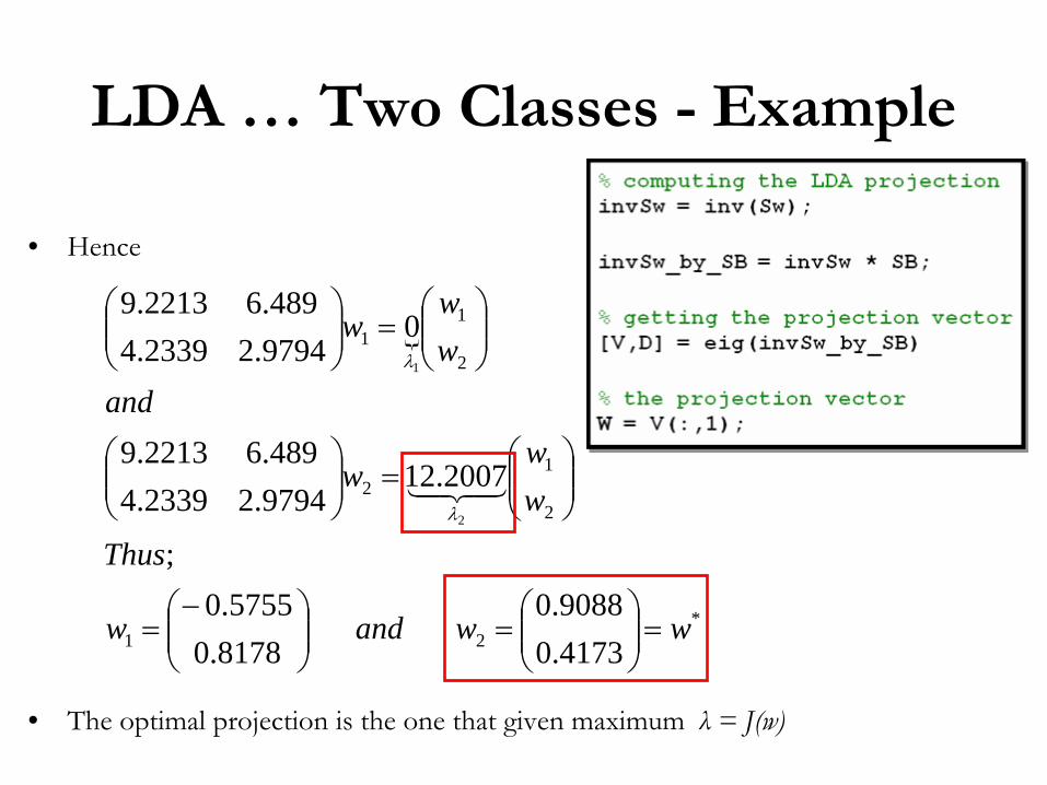
Example

• Hence

• The optimal projection is the one that given maximum λ

= J(w)

{

*21

2

12

2

11

4173.09088.0

8178.05755.0

;

2007.129794.22339.4489.62213.9

09794.22339.4489.62213.9

2

1

wwandw

Thus

ww

w

andww

w

=⎟⎟⎠

⎞⎜⎜⎝

⎛=⎟⎟

⎠

⎞⎜⎜⎝

⎛−=

⎟⎟⎠

⎞⎜⎜⎝

⎛=⎟⎟

⎠

⎞⎜⎜⎝

⎛

⎟⎟⎠

⎞⎜⎜⎝

⎛=⎟⎟

⎠

⎞⎜⎜⎝

⎛

43421λ

λ

LDA …

Two Classes -

Example

( )

⎟⎟⎠

⎞⎜⎜⎝

⎛=

⎟⎟⎠

⎞⎜⎜⎝

⎛−−

⎟⎟⎠

⎞⎜⎜⎝

⎛=

⎥⎦

⎤⎢⎣

⎡⎟⎟⎠

⎞⎜⎜⎝

⎛−⎟⎟

⎠

⎞⎜⎜⎝

⎛⎟⎟⎠

⎞⎜⎜⎝

⎛−

−=−=

−−

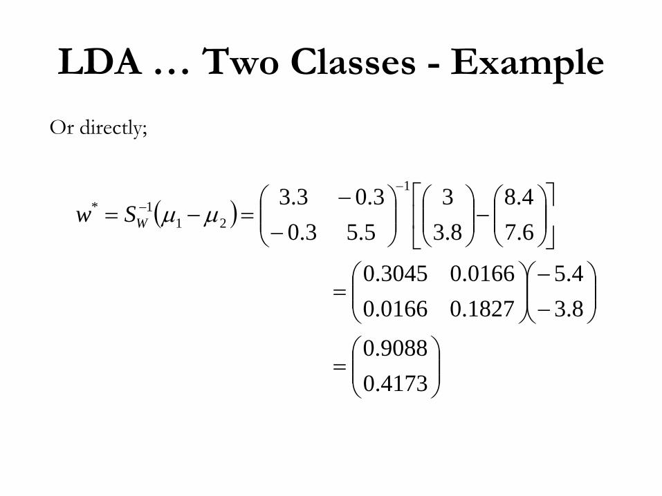
4173.09088.0

8.34.5

1827.00166.00166.03045.0

6.74.8

8.33

5.53.03.03.3 1

211* μμWSw

Or directly;

LDA -

Projection

-4 -3 -2 -1 0 1 2 3 4 5 60

0.05

0.1

0.15

0.2

0.25

0.3

0.35

y

p(y

|w

i)

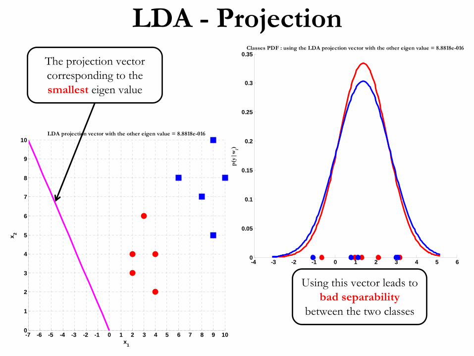
Classes PDF : using the LDA projection vector with the other eigen value = 8.8818e-016

-7 -6 -5 -4 -3 -2 -1 0 1 2 3 4 5 6 7 8 9 100

1

2

3

4

5

6

7

8

9

10

x1

x 2

LDA projection vector with the other eigen value = 8.8818e-016

The projection vector corresponding to the smallest

eigen

value

Using this vector leads to bad separability

between the two classes

LDA -

Projection

0 5 10 150

0.05

0.1

0.15

0.2

0.25

0.3

0.35

0.4

y

p(y

|w

i)

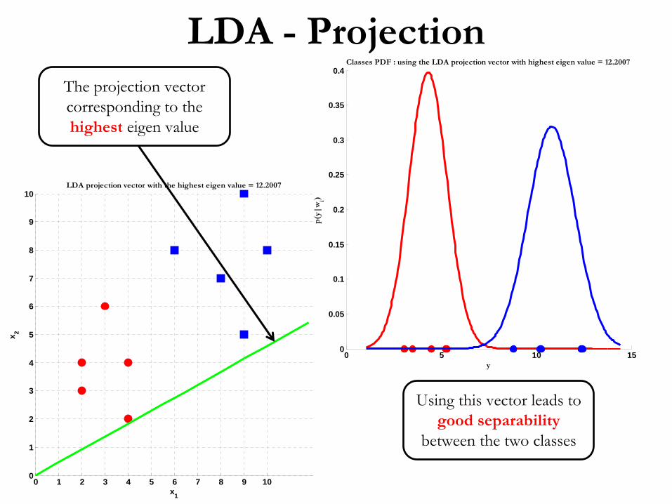
Classes PDF : using the LDA projection vector with highest eigen value = 12.2007

0 1 2 3 4 5 6 7 8 9 100

1

2

3

4

5

6

7

8

9

10

x1

x 2

LDA projection vector with the highest eigen value = 12.2007

The projection vector corresponding to the highest

eigen

value

Using this vector leads to good separability

between the two classes

LDA …

C-Classes

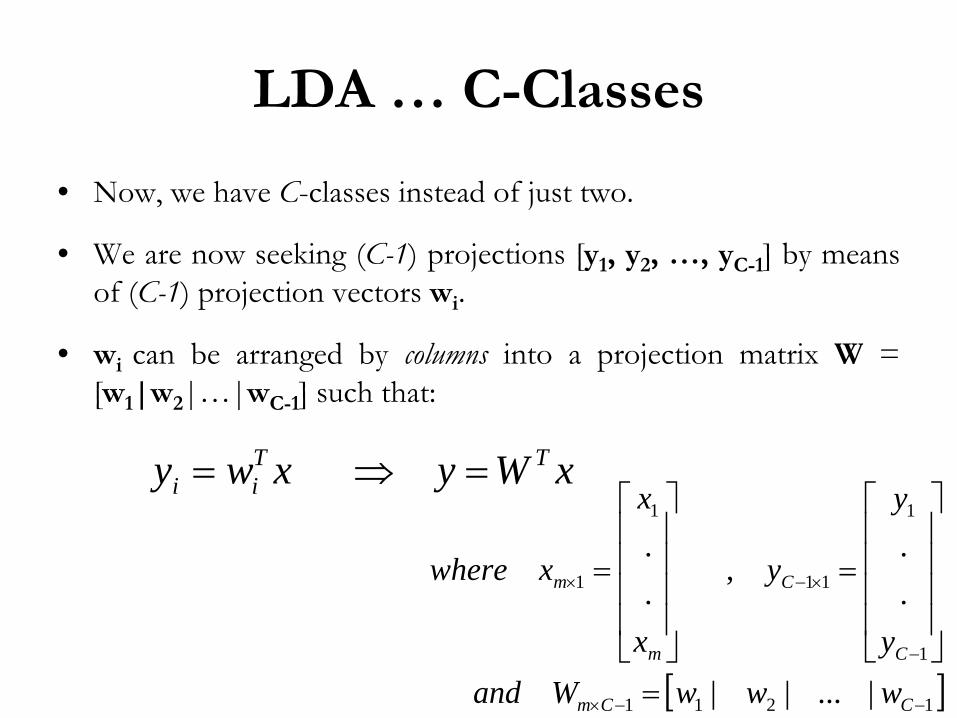
• Now, we have C-classes instead of just two.

• We are now seeking (C-1) projections [y1

, y2

, …, yC-1

] by means of (C-1) projection vectors wi

.

• wi

can be arranged by columns

into a projection matrix W

=

[w1

|w2

|…|wC-1

] such that:

[ ]1211

1

1

11

1

1

|...||

.

.,

.

.

−−×

−

×−×

=

⎥⎥⎥⎥

⎦

⎤

⎢⎢⎢⎢

⎣

⎡

=

⎥⎥⎥⎥

⎦

⎤

⎢⎢⎢⎢

⎣

⎡

=

CCm

C

C

m

m

wwwWandy

y

y

x

x

xwhere

xWyxwy TTii =⇒=

LDA …

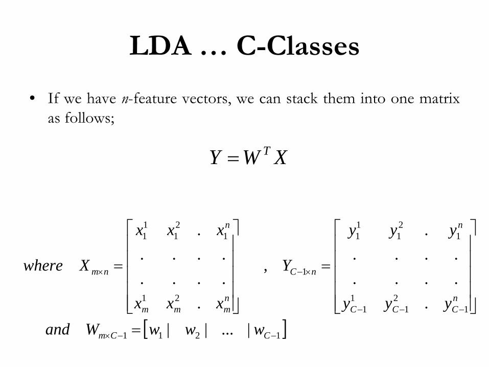
C-Classes

• If we have n-feature vectors, we can stack them into one matrix as follows;

[ ]1211

12

11

1

121

11

1

21

121

11

|...||.

....

.....

,

.........

.

−−×

−−−

×−×

=⎥⎥⎥⎥⎥

⎦

⎤

⎢⎢⎢⎢⎢

⎣

⎡

=

⎥⎥⎥⎥⎥

⎦

⎤

⎢⎢⎢⎢⎢

⎣

⎡

=

CCm

nCCC

n

nC

nmmm

n

nm

wwwWandyyy

yyy

Y

xxx

xxx

Xwhere

XWY T=

LDA –

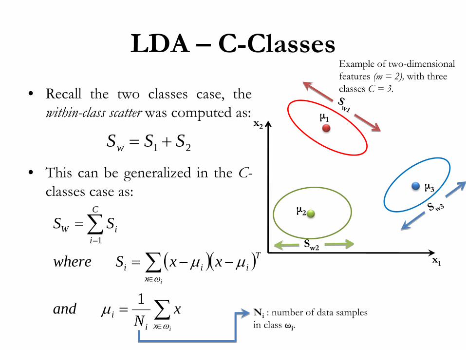
C-Classes

• Recall the two classes case, the within-class scatter was computed as:

• This can be generalized in the C- classes case as:

21 SSSw +=

( )( )

∑

∑

∑

∈

∈

=

=

−−=

=

i

i

xii

Ti

xii

C

iiW

xN

and

xxSwhere

SS

ω

ω

μ

μμ

1

1

x1

x2μ1

μ2

μ3

Sw1

S w3

Sw2

Example of two-dimensional features (m = 2),

with three classes C = 3.

Ni

: number of data samples in class ωi

.

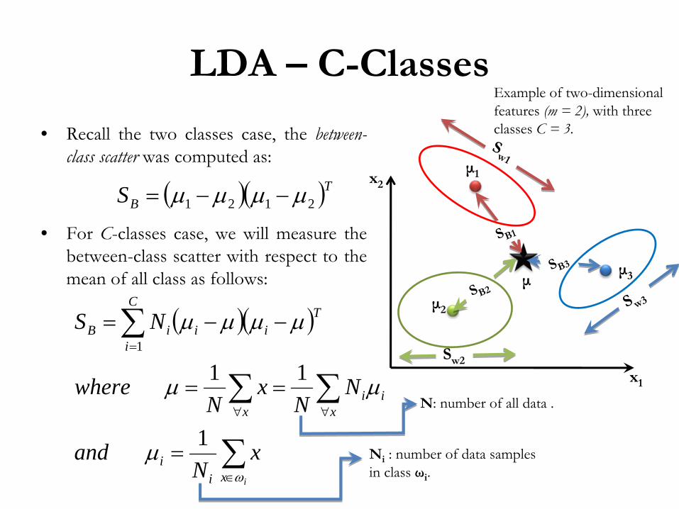
LDA –

C-Classes

• Recall the two classes case, the between-

class scatter was computed as:

• For C-classes case, we will measure the between-class scatter with respect to the mean of all class as follows:

( )( )

∑

∑∑

∑

∈

∀∀

=

=

==

−−=

ixii

xii

x

C

i

TiiiB

xN

and

NN

xN

where

NS

ω

μ

μμ

μμμμ

1

111

( )( )TBS 2121 μμμμ −−=

x1

x2μ1

μ2

μ3

Sw1

S w3

Sw2

μ

SB1

SB3

SB2

Example of two-dimensional features (m = 2),

with three classes C = 3.

Ni

: number of data samples in class ωi

.

N: number of all data .

LDA –

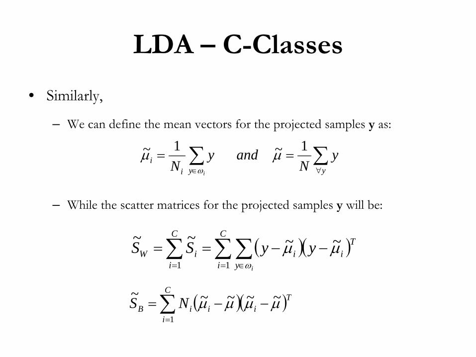
C-Classes

• Similarly,

– We can define the mean vectors for the projected samples y

as:

– While the scatter matrices for the projected samples y

will be:

∑∑∀∈

==yyi

i yN

andyN

i

1~1~ μμω

( )( )∑∑∑= ∈=

−−==C

i

Ti

yi

C

iiW yySS

i11

~~~~ μμω

( )( )∑=

−−=C

i

TiiiB NS

1

~~~~~ μμμμ

LDA –

C-Classes

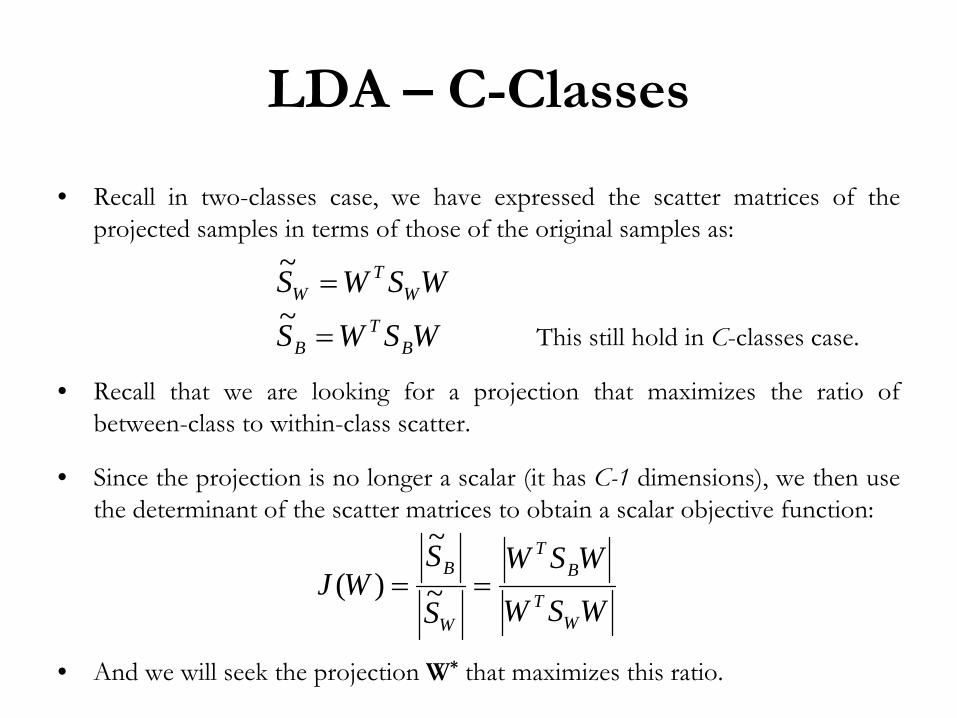
• Recall in two-classes case, we have expressed the scatter matrices of the projected samples in terms of those of the original samples as:

This still hold in C-classes case.

• Recall that we are looking for a projection that maximizes the ratio of between-class to within-class scatter.

• Since the projection is no longer a scalar (it has C-1

dimensions), we then use the determinant of the scatter matrices to obtain a scalar objective function:

• And we will seek the projection W*

that maximizes this ratio.

WSWS

WSWS

BT

B

WT

W

=

=~

~

WSW

WSW

S

SWJ

WT

BT

W

B== ~

~)(

LDA –

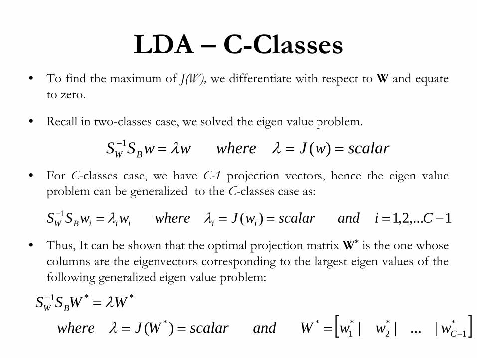
C-Classes• To find the maximum of J(W), we differentiate with respect to W

and equate to zero.

• Recall in two-classes case, we solved the eigen

value problem.

• For C-classes case, we have C-1

projection vectors, hence the eigen

value problem can be generalized to the C-classes case as:

• Thus, It can be shown that the optimal projection matrix W*

is the one whose columns are the eigenvectors corresponding to the largest eigen

values of the following generalized eigen

value problem:

1,...2,1)(1 −====− CiandscalarwJwherewwSS iiiiiBW λλ

scalarwJwherewwSS BW ===− )(1 λλ

[ ]*1

*2

*1

**

**1

|...||)( −

−

===

=

C

BW

wwwWandscalarWJwhere

WWSS

λ

λ

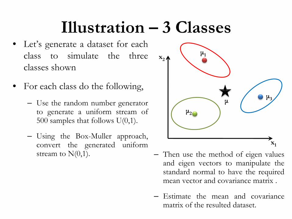
Illustration –

3 Classes• Let’s

generate a dataset for each

class to simulate the three classes shown

• For each class do the following,

– Use the random number generator to generate a uniform stream of 500 samples that follows U(0,1).

– Using the Box-Muller approach, convert the generated uniform stream to N(0,1).

x1

x2μ1

μ2

μ3μ

– Then use the method of eigen

values and eigen

vectors to manipulate the standard normal to have the required mean vector and covariance matrix .

– Estimate the mean and covariance matrix of the resulted dataset.

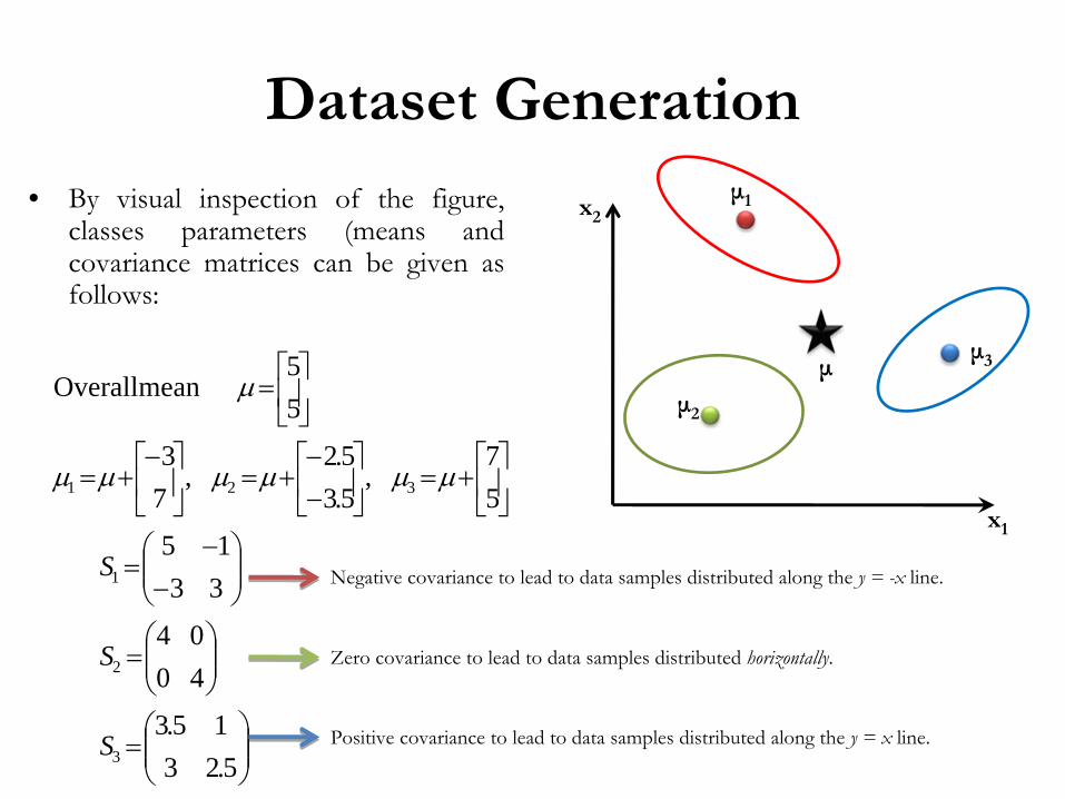
• By visual inspection of the figure, classes parameters (means and covariance matrices can be given as follows:

Dataset Generation

x1

x2μ1

μ2

μ3μ

⎟⎟⎠

⎞⎜⎜⎝

⎛=

⎟⎟⎠

⎞⎜⎜⎝

⎛=

⎟⎟⎠

⎞⎜⎜⎝

⎛−

−=

⎥⎦

⎤⎢⎣

⎡+=⎥

⎦

⎤⎢⎣

⎡−−

+=⎥⎦

⎤⎢⎣

⎡−+=

⎥⎦

⎤⎢⎣

⎡=

5.2315.3

4004

3315

57

,5.35.2

,73

55

mean Overall

3

2

1

321

S

S

S

μμμμμμ

μ

Zero covariance to lead to data samples distributed horizontally.

Positive covariance to lead to data samples distributed along the y = x line.

Negative covariance to lead to data samples distributed along the y = -x line.

In Matlab ☺

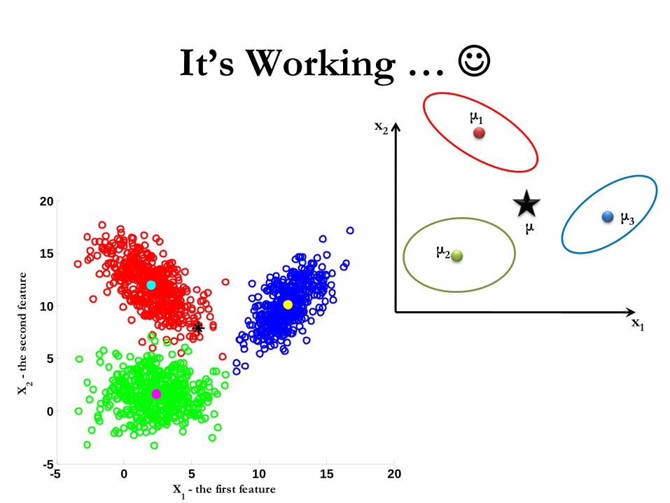
It’s Working … ☺

-5 0 5 10 15 20-5

0

5

10

15

20

X1 - the first feature

X2 -

th

e se

con

d f

eatu

re

x1

x2μ1

μ2

μ3μ

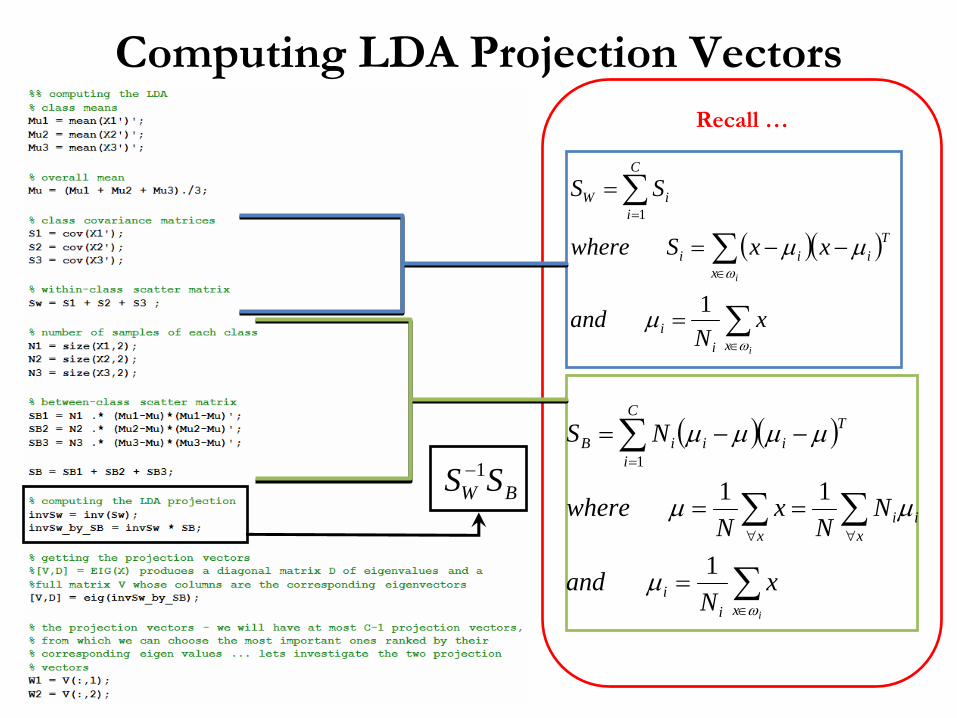
Computing LDA Projection Vectors

( )( )

∑

∑∑

∑

∈

∀∀

=

=

==

−−=

ixii

xii

x

C

i

TiiiB

xN

and

NN

xN

where

NS

ω

μ

μμ

μμμμ

1

111

( )( )

∑

∑

∑

∈

∈

=

=

−−=

=

i

i

xii

Ti

xii

C

iiW

xN

and

xxSwhere

SS

ω

ω

μ

μμ

1

1

Recall …

BW SS 1−

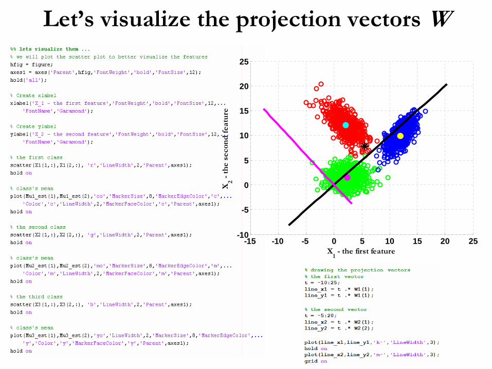
Let’s visualize the projection vectors W

-15 -10 -5 0 5 10 15 20 25-10

-5

0

5

10

15

20

25

X1 - the first feature

X2 -

th

e se

con

d f

eatu

re

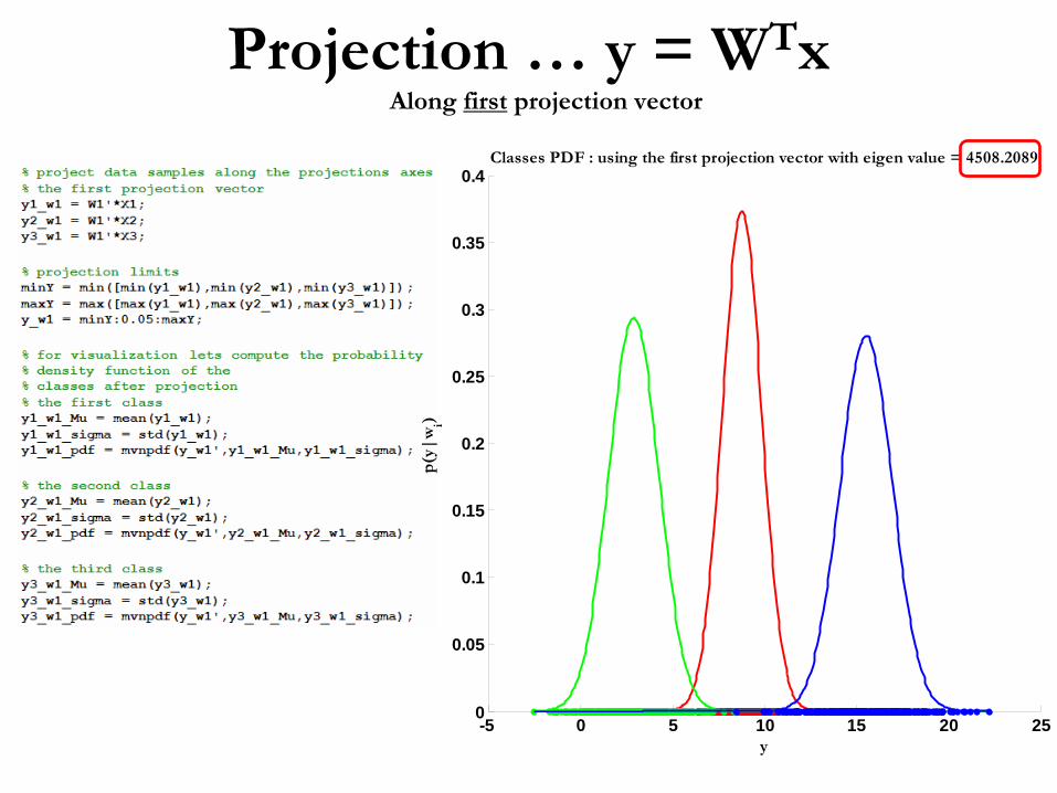
Projection …

y = WTxAlong first

projection vector

-5 0 5 10 15 20 250

0.05

0.1

0.15

0.2

0.25

0.3

0.35

0.4

y

p(y

|w

i)

Classes PDF : using the first projection vector with eigen value = 4508.2089

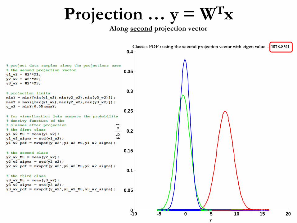
Projection …

y = WTxAlong second

projection vector

-10 -5 0 5 10 15 200

0.05

0.1

0.15

0.2

0.25

0.3

0.35

0.4

y

p(y

|w

i)

Classes PDF : using the second projection vector with eigen value = 1878.8511

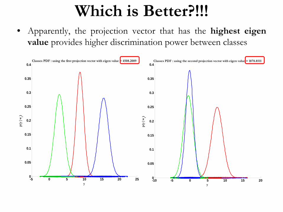
Which is Better?!!!• Apparently, the projection vector that has the highest eigen

value provides higher discrimination power between classes

-10 -5 0 5 10 15 200

0.05

0.1

0.15

0.2

0.25

0.3

0.35

0.4

y

p(y

|w

i)

Classes PDF : using the second projection vector with eigen value = 1878.8511

-5 0 5 10 15 20 250

0.05

0.1

0.15

0.2

0.25

0.3

0.35

0.4

y

p(y

|w

i)

Classes PDF : using the first projection vector with eigen value = 4508.2089

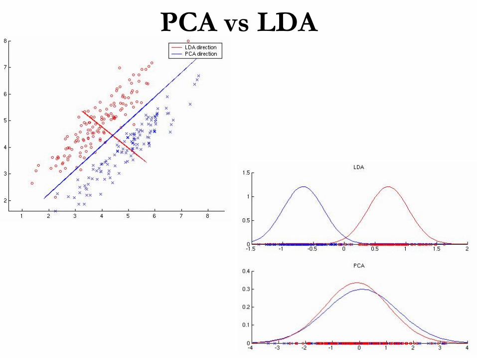
PCA vs

LDA

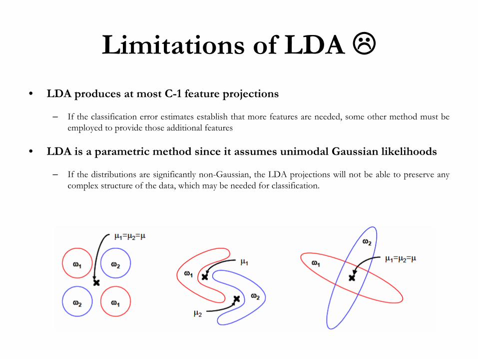
Limitations of LDA

• LDA produces at most C-1 feature projections

– If the classification error estimates establish that more features are needed, some other method must be employed to provide those additional features

• LDA is a parametric method since it assumes unimodal

Gaussian likelihoods

– If the distributions are significantly non-Gaussian, the LDA projections will not be able to preserve any complex structure of the data, which may be needed for classification.

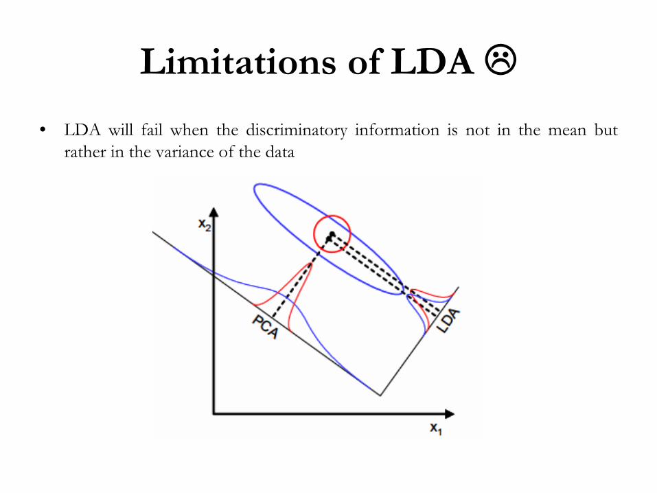
Limitations of LDA

• LDA will fail when the discriminatory information is not in the mean but rather in the variance of the data

Thank You