A Tutorial on Computational Learning Theory Presented …honavar/colt-tutorial.pdf · A Tutorial on...
43
A Tutorial on Computational Learning Theory Presented at Genetic Programming 1997 Stanford University, July 1997 Vasant Honavar Artificial Intelligence Research Laboratory Department of Computer Science [email protected] Iowa State University, Ames, Iowa 50011 http://www.cs.iastate.edu/~honavar/aigroup.html
Transcript of A Tutorial on Computational Learning Theory Presented …honavar/colt-tutorial.pdf · A Tutorial on...

A Tutorial on Computational Learning TheoryPresented at Genetic Programming 1997
Stanford University, July 1997
Vasant HonavarArtificial Intelligence Research Laboratory
Department of Computer [email protected]
Iowa State University, Ames, Iowa 50011http://www.cs.iastate.edu/~honavar/aigroup.html

What are learning systems?
Systems that improve their performance one or more tasks with experience in their environment
Examples: Pattern recognizers, adaptive control systems, adaptive intelligent agents, etc.

Computational Models of Learning
• Model of the Learner: Computational capabilities, sensors, effectors, knowledge representation, inference mechanisms, prior knowledge, etc.
• Model of the Environment: Tasks to be learned, information sources (teacher, queries, experiments), performance measures
• Key questions: Can a learner with a certain structure learn a specified task in a particular environment? Can the learner do so efficiently? If so, how? If not, why not?

Computational Models of Learning
• Theories of Learning: What is it good for?• Mistake bound model• Maximum Likelihood model• PAC (Probably Approximately Correct) model• Learning from simple examples• Concluding remarks

• To make explicit relevant aspects of the learner and the environment
• To identify easy and hard learning problems (and the precise conditions under which they are easy or hard)
• To guide the design of learning systems• To shed light on natural learning systems• To help analyze the performance of learning systems
Theories of Learning: What are they good for?

Mistake bound Model
Example: Given an arbitrary, noise-free sequence of labeled examples <X1,C(X1)>,<X2,C(X2)>...of an unknown binary conjunctive concept C over {0,1}N, the learner's task is to predict C(X) for a given X.
Theorem: Exact online learning of conjunctive concepts can be accomplished with at most (N+1) prediction mistakes.

Mistake bound model
Algorithm• Initialize L={X1, ~X1, .... ~XN}• Predict according to match between an instance
and the conjunction of literals in L• Whenever a mistake is made on a positive
example, drop the offending literals from LEg: <0111, 1> will result in L = {~ X1, X2, X3, X4}
<1110, 1> will yield L = {X2, X3}

Mistake bound model
Proof of Theorem 1:• No literal in C is ever eliminated from L• Each mistake eliminates at least one literal from L• The first mistake eliminates N of the 2N literals• Conjunctive concepts can be learned with at most
(N+1) mistakes Conclusion: Conjunctive concepts are easy to learn
in the mistake bound model

Optimal Mistake Bound Learning Algorithms
Definition: An optimal mistake bound mbound(C) for a concept classs C is the lowest possible mistake bound in the worst case (considering all concepts in C, and all possible sequences of examples).
Definition: An optimal learning algorithm for a concept class C (in the mistake bound framework) is one that is guaranteed to exactly learn any concept in C, using any noise-free example sequence, with at most O(mbound(C)) mistakes.
Theorem:
≤≤
mbound( ) lg| |C C≤

The Halving Algorithm
Definition: The version space
Definition: The halving algorithm predicts according to the majority of concepts in the current version space and a mistake results in elimination of all the offending concepts from the version space
Fine print: The halving algorithm may not be efficiently implementable.
{ }iV C C= ∈C| is consistent with the first i examples

The Halving Algorithm
The halving algorithm can be practical if there is a way to compactly represent and efficiently manipulate the version space.
Question: Are there any efficiently implementable optimal mistake bound learning algorithms?
Answer: Littlestone's algorithm for learning monotone disjunctions of at most k of n literals using the hypothesis class of threshold functions with at most (k lg n) mistakes.

Bounding the prediction error
• Mistake bound model bounds the number of mistakes that the learner will ever make before exactly learning a concept, but not the prediction error after having seen a certain number of examples.
• Mistake bound model assumes that the examples are chosen arbitrarily - in the worst case, by a smart, adversarial teacher. It might often be satisfactory to assume randomly drawn examples

Probably Approximately Correct Learning
Oracle
Samples
Instance Distribution
LearnerExamples
Concept

Probably Approximately Correct Learning
Consider:• An instance space X• A concept space • A hypothesis space• An unknown, arbitrary, not necessarily
computable, stationary probability distribution Dover the instance space X
{ }{ }C = →C: ,X 0 1
{ }{ }H = →h : ,X 0 1

PAC Learning
• The oracle samples the instance space according to D and provides labeled examples of an unknown concept C to the learner
• The learner is tested on samples drawn from the instance space according to the same probability distribution D
• The learner's task is to output a hypothesis h from H that closely approximates the unknown concept C based on the examples it has encountered

PAC Learning
• In the PAC setting, exact learning (zero error approximation) cannot be guaranteed
• In the PAC setting, even approximate learning (with bounded non-zero error) cannot be guaranteed 100% of the time
Definition: The error of a hypothesis h with respect to a target concept C and an instance distribution Dis given by ProbD[ ]C X h X( ) ( )≠

PAC Learning
Definition: A concept class C is said to be PAC-learnable using a hypothesis class H if there exists a learning algorithm L such that for all concepts in C, for all instance distributions D on an instance space X, , L, when given access to the Example oracle, produces, with probability at least , a hypothesis h from H with error no more than (Valiant, 1984)
( )∀ < <ε δ ε δ, , 0 1
( )1−δε

Efficient PAC Learning
Definition: C is said to be efficiently PAC-learnable if L runs in time that is polynomial in N (size of the instance representation), size(C) (size of the concept representation), and
Remark Note that lower error or increased confidence require more examples.
Remark: In order for a concept class to be efficiently PAC-learnable, it should be PAC-learnable using a random sample of size polynomial in the relevant parameters.
1ε
1δ

Sample complexity of PAC Learning
Definition: A consistent learner is one that returns some hypothesis h from the hypothesis class H that is consistent with a random sequence of m examples.
Remark: A consistent learner is a MAP learner (one that returns a hypothesis that is most likely given the training data) if all hypotheses are a-priori equally likely
Theorem: A consistent learner is guranteed to be PAC if the number of samples
m >1ε δ
l nH

Sample Complexity of PAC Learning
Proof: Consider a hypothesis h that is not a PAC approximation of an unknown concept C. Clearly, error of h, or the probability that h is wrong on a random instance is at least . The probability of h being wrong on m independently drawn random examples is at least . For PAC learning, we want to make sure that the probability of L returning such a bad hypothesis is small.
( )1− ε
( )m1−ε
( )Hm1− <ε δ
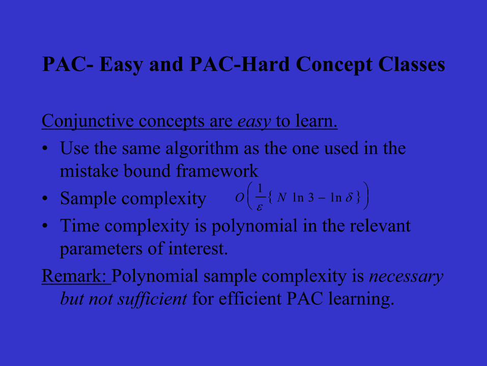
PAC- Easy and PAC-Hard Concept Classes
Conjunctive concepts are easy to learn.• Use the same algorithm as the one used in the
mistake bound framework• Sample complexity • Time complexity is polynomial in the relevant
parameters of interest.Remark: Polynomial sample complexity is necessary
but not sufficient for efficient PAC learning.
{ }O N1
3ε
δln ln−

PAC-Easy and PAC-Hard Concept Classes
Theorem: 3-term DNF concept class (disjunctions of at most 3 conjunctions) are not efficiently PAC-learnable using the same hypothesis class (although it has polynomial sample complexity) unless P=NP.
Proof: By polynomial time reduction of graph 3-colorability (a well-known NP-complete problem) to the problem of deciding whether a given set of labeled examples is consistent with some 3-term DNF formula.

Transforming Hard Problems to Easy ones
Theorem: 3-term DNF concepts are efficiently PAC-learnable using 3-CNF (conjunctive normal form with at most 3 literals per clause) hypothesis class.
Proof: Transform each example over N boolean variables
into a corresponding example over N3 variables (one for each possible clause in a 3-CNF formula).
The problem reduces to learning a conjunctive concept over the transformed instance space.
3 - term DNF 3 - CNF⊆

Transforming Hard Problems to Easy ones
Theorem For any k-term DNF are efficiently PAC-learnable using the k-CNF hypothesis class.
Remark: In this case, enlarging the search space by using a hypothesis class that is larger than strictly necessary, actually makes the problem easy!
Remark: No, we have not proved that P=NP.Summary:
k ≥ 2
Conjunctive k-term DNF k-CNF CNF Easy Hard Easy Hard
⊆ ⊆ ⊆

Inductive Bias: Occam's Razor
Occam's razor: Keep it simple, stupid!An Occam learning algorithm returns a simple or succinct
hypothesis that is consistent with the training data.Definition: Let be constants. A learning
algorithm L is said to be an Occam algorithm for a concept class C using a hypothesis class H if L, given m random examples of an unknown concept , outputs a hypothesis such that h is consistent with the examples and
α β≥ ≤ <0 1 0&α β−
C ∈Ch ∈H
{ }size h Nsize c m( ) ( )≤α β

Sample complexity of an Occam Algorithm
Theorem: An Occam algorithm is guaranteed to be PAC if the number of samples
Proof: omitted.
( )m O
Nsize c= +
−
1 1
11
ε δ ε
α β
lg( )

Occam algorithm is PAC for K-decision lists
Theorem: For any fixed k, the concept class of k-decision lists (nested if-then-else statements where each if condition is a conjunction of at most k of N literals and their negations) is efficiently PAC-learnable using the the same hypothesis class.
Remark: K-decision lists constitute the most expressive boolean concept class over the boolean instance space {0,1}N that are known to be efficiently PAC learnable.

PAC Learning of Infinite Concept Classes
Sample complexity results can be derived for concepts defined over .
Remark: Note that the cardinality of concept and hypothesis classes can now be infinite (e.g., in the case of threshold functions over ).
Solution: Instead of the cardinality of concept class, use the Vapnik-Chervonenkis dimension (VC dimension) of the concept class to compute sample complexity
ℜN
ℜN

VC Dimension and Sample Complexity
Definition: A set S of instances is shattered by a hypothesis class H if and only if for every dichotomy of S, there exists a hypothesis in H that is consistent with the dichotomy.
Definition: The VC-dimension V(H), of a hypothesis class H defined over an instance space X is the cardinality of the largest subset of X that is shattered by H. If arbitrarily large finite subsets of X can be shattered by H, V(H)= ∞

VC Dimension and Sample Complexity
Example: Let the instance space X be the 2-dimensional Euclidian space. Let the hypothesis space H be the set of linear 1-dimensional hyperplanes in the 2-dimensional Euclidian space.
Then V(H)=3 (a set of 3 points can be shattered by a hyperplane as long as they are not colinear but a set of 4 points cannot be shattered).

VC Dimension and Sample Complexity
Theorem: The number m of random examples needed for PAC learning of a concept class C of VC dimension V(C) = d is given by
Corollary: Acyclic, layered multi-layer networks of s threshold logic units, each with r inputs, has VC dimension
m O d= +
1 1 1ε δ ε
lg lg
≤ +2 1( ) lg( )r s es

Using a Weak learner for PAC Learning
PAC learning requires learning under all distributions, for all choices of error and confidence parameters. Suppose we are given a weak learning algorithm for concept class C that works for a fixed error and/or a fixed confidence. Can we use it for PAC learning of C?
YES! (Kearns & Vazirani, 94; Natarajan, 92)

Learning from Simple Examples
Question:• Can we relax the requirement of learning under
all probability distributions over the instance space (including extremely pathological distributions) by limiting the class of distributions to a useful subset of all possible distributions?
• What are the implications of doing so on the learnability of concept classes that are PAC-hard?
• What probability distributions are natural?

Learning from Simple Examples
Intuition: Suppose mother nature is kind to us:Simple instances are more likely to be made
available to the learner.Question: How can we formalize this intuitive
notion?Answer: Kolmogorov complexity offers a natural
measure of descriptional complexity of an instance

Kolmogorov Complexity
Definition: Kolmogorov complexity of an object relative to a universal Turing machine M is the length (measured in number of bits) of the shortest program which when executed on M, prints out and halts.
Remark: Simple objects (e.g., a string of all zeros) have low Kolmogorov complexity.
γ
γ( ) ( ) ( ){ }K l Mγ π π γ
π= =min |

Kolmogorov Complexity
Definition: The conditional Kolmogorov complexity of given is the length of the shortest program for a universal Turing machine M which, given , outputs .
Remark: Remark: Kolmogorov complexity is machine-
independent (modulo an additive constant).
γ λ
λπ
γ
( ) ( )K Kγ λ γ| ≤

Universal Distribution
Definition: The universal probability distribution over an instance space X is defined by:
where is a normalization constant.
Definition: A distribution D is simple if it is multiplicatively dominated by the universal distribution, that is, there exists a constant such that
Remark: All computable distributions (including gaussian, poisson, etc. with finite precision parameters) are simple.
( )U
K XXD ( ) = −η2 η∀ ∈X X
σ ( ) ( )σ U X XD D≥

PAC Learning Under Simple Distributions
Theorem: A concept class C defined over a discrete instance space is polynomially PAC-learnable under the universal distribution iff it is polynomially PAC-learnable under each simple distribution, provided, during the learning phase, the samples are drawn according to the universal distribution. (Li & Vitanyi, 91)
Remarks: This raises the possibility of learning under all simple distributions by sampling examples according to the universal distribution. But universal distribution is not computable. Is nature characterized by universal distribution? Can we approximate universal distribution?

Learning from Simple Examples
Suppose a knowledgeable teacher provides simple examples (i.e., examples with low Kolmogorov complexity conditioned on the teacher's knowledge of the concept to be learned).
More precisely, where r is a suitable representation of the unknown
concept and is a normalization constant.Definition: Let SS , a set of simple examples, that is,
( )Dr rK X rX = −η 2 ( | )
ηr
( )∀ ∈ ≤X S K X r sizeof rS lg( | ) ( )µµ

Learning from Simple Examples
Definition (informal): A representative sample SR is one that contains all the information necessary for identifying an unknown concept.
Example: To learn a finite state machine, a representative examples provide information about all the state transitions.
Theorem: If there exists a representative set of simpleexamples for each concept in a concept class C, then C is PAC learnable under distribution Dr. (Denis et al., 96)

Learning from Simple Examples
Theorem: The class of DFA whose canonical representations have at most Q states are polynomially exactly learnable when examples are provided from a sample drawn according to Dr when Q is known. (Parekh & Honavar, 97)
Theorem: The class of DFA are probably approximately learnable under Dr (Parekh & Honavar, 97).
Remark: These are encouraging results in light of the strong evidence against efficient PAC learnability of DFA (Kearns and Vazirani, 1994)

Concluding remarks
• PAC-Easy learning problems lend themselves to a variety of efficient algorithms.
• PAC-Hard learning problems can often be made PAC-easy through appropriate instance transformation and choice of hypothesis space
• Occam's razor often helps• Weak learning algorithms can often be used for strong
learning• Learning under restricted classes of instance distributions
(e.g., universal distribution) offers new possibilities

Bibliography
1 Honavar, V. http://www.cs.iastate.edu/~honavar/cs673.s96.html2 Kearns, M.J. & Vazirani, U.V. An Introduction to Computational
Learning Theory. Cambridge, MA: MIT Press. 1994.3 Langley, P. Elements of Machine Learning. Palo Alto, CA: Morgan
Kaufmann. 1995.4 Li, M. & Vitanyi, P. Kolmogorov Complexity and its Applications.
New York: Springer-Verlag. 1997.5 Mitchell, T. Machine Learning. New York: McGraw Hill. 1997.6 Natarajan, B.K. Machine Learning: A Theoretical Approach. Palo
Alto, CA: Morgan Kaufmann, 1992.