A Tutorial on Automated Text Categorisation

Fabrizio SebastianiIstituto di Elaborazione dell’Informazione

Consiglio Nazionale delle RicercheVia S. Maria, 46 - 56126 Pisa (Italy)E-mail: fabrizio@iei.pi.cnr.it

Abstract

The automated categorisation (or classification) of texts into topical categories has a long his-tory, dating back at least to 1960. Until the late ’80s, the dominant approach to the probleminvolved knowledge-engineering automatic categorisers, i.e. manually building a set of rulesencoding expert knowledge on how to classify documents. In the ’90s, with the booming pro-duction and availability of on-line documents, automated text categorisation has witnessedan increased and renewed interest. A newer paradigm based on machine learning has super-seded the previous approach. Within this paradigm, a general inductive process automaticallybuilds a classifier by “learning”, from a set of previously classified documents, the character-istics of one or more categories; the advantages are a very good effectiveness, a considerablesavings in terms of expert manpower, and domain independence. In this tutorial we look atthe main approaches that have been taken towards automatic text categorisation within thegeneral machine learning paradigm. Issues of document indexing, classifier construction, andclassifier evaluation, will be touched upon.

1 A definition of the text categorisation task

Document categorisation (or classification) may be seen as the task of determining an assignmentof a value from {0,1} to each entry of the decision matrix

d1 . . . . . . dj . . . . . . dn

c1 a11 . . . . . . a1j . . . . . . a1n

. . . . . . . . . . . . . . . . . . . . . . . .ci ai1 . . . . . . aij . . . . . . ain

. . . . . . . . . . . . . . . . . . . . . . . .cm am1 . . . . . . amj . . . . . . amn

where C = {c1, . . . , cm} is a set of pre-defined categories, and D = {d1, . . . , dn} is a set of doc-uments to be categorised (sometimes called “requests”). A value of 1 for aij is interpreted as adecision to file dj under ci, while a value of 0 is interpreted as a decision not to file dj under ci.

Fundamental to the understanding of this task are two observations:

• the categories are just symbolic labels. No additional knowledge of their “meaning” isavailable to help in the process of building the categoriser; in particular, this means that the“text” constituting the label (e.g. Sports in a news categorisation task) cannot be used;

• the attribution of documents to categories should, in general, be attributed on the basisof the content of the documents, and not on the basis of metadata (e.g. publication date,

1

document type, etc.) that may be available from an external source. This means that thenotion of relevance of a document to a category is inherently subjective1.

Different constraints may be enforced on the categorisation task, depending on the application:we may want that

1. {≤ 1 | 1 | ≥ 1 | . . . } elements of C must be assigned to each element of D. When exactlyone category is assigned to each document (as e.g. in [28, 43]), this is often referred to asthe non-overlapping categories case.

2. each element of C must be assigned to {≤ 1 | 1 | ≥ 1 | . . . } elements of D.

The techniques we will consider here are applicable irrespectively of whether any of these con-straints are enforced or not.

1.1 Category- or document-pivoted categorisation

An important distinction is whether we want to fill the matrix one row at a time (category-pivotedcategorisation – CPC), or fill the it one column at a time (document-pivoted categorisation – DPC).This distinction is mostly pragmatic rather than conceptual, but is important in the sense thatthe sets C of categories and D of documents are not always available in their entirety right fromthe start.

DPC is thus suitable when documents might become available one at a time over a long spanof time, e.g. in the case a user submits one document at a time for categorisation, rather thansubmitting a whole batch of them all at once. In this case, sometimes the categorisation tasktakes the form of ranking the categories in decreasing order of their estimated appropriateness fordocument d; because of this, CPC is sometimes called category-ranking classification or on-lineclassification [50].

CPC is instead suitable if we consider the possibility that a new category cm+1 is inserted intoa previously existing set of categories C = {c1, . . . , cm} after a number of documents have alreadybeen categorised under C, which means that these documents need to be categorised under cm+1

too. In this case, sometimes the categorisation task takes the form of ranking the documentsin decreasing order of their estimated appropriateness for category cm+1; symmetrically to theprevious case, DPC may also be called document-ranking classification.

CPC is more commonly used than DPC, as the case in which documents are submitted oneat a time is somehow more common than the case in which newer categories dynamically cropup. However, although some specific techniques apply to one and not to the other (e.g. theproportional thresholding method discussed in Section 6, which applies only to CPC), this ismore the exception than the rule: most of the techniques we will discuss in this paper allow theconstruction of classifiers capable of working in either mode.

2 Applications of document categorisation

Automatic text categorisation goes back at least to the early ’60, with the seminal work byMaron [29]. Since then, it has been used in a number of different applications. In the following,we briefly review the most important ones.

1This is exemplified by the well-known phenomenon of inter-indexer inconsistency [5]: when two differenthumans must take a decision on whether to categorise document d under category c, they may disagree. Notethat the above-mentioned notion of relevance of a document to a category is basically the notion of relevance of adocument to an information need, as from information retrieval [41].

2

2.1 Automatic indexing for Boolean information retrieval systems

The first use to which automatic categorisers were put at, and the application that spawned mostof the early research in the field, is that of automatic document indexing for use in informationretrieval (IR) systems relying on a controlled dictionary. The most prominent example of such IRsystems is, of course, that of Boolean systems. In these systems, each document is assigned one ormore keywords or keyphrases describing its content, where these keywords and keyphrases belongto a finite set of words, called controlled dictionary) and often consisting of a hierarchical thesaurus(e.g. the NASA thesaurus for the aerospace discipline [34], or the MESH thesaurus covering themedical field [35]). Usually, this assignment is performed by trained human indexers, and is thusan extremely costly activity.

If the entries in the thesaurus are viewed as categories, document indexing becomes an instanceof the document categorisation task, and may thus be addressed by the automatic techniques de-scribed in this paper. Concerning Point 1 in Section 1, note that in this case a typical constraintmay be that l1 ≤ x ≤ l2 keywords are assigned to each document. Document-pivoted categorisa-tion might typically be the best option, so that documents are categorised on a first come, firstserved basis.

Various automatic document categorisers explicitly addressed at the document indexing appli-cation have been described in the literature; see e.g. [4, 10, 12].

2.2 Document organisation

In general, all issues pertaining to document organisation and filing , be it for purposes of personalorganisation or document repository structuring, may be addressed by automatic categorisationtechniques. For instance, at the offices of a newspaper, incoming “classified” ads should be, priorto publication, categorised under the categories used in the categorisation scheme adopted by thenewspaper; typical categories might be e.g. Personals, Cars for sale, Real estate, . . . . While mostnewspapers would handle this application manually, those dealing with a high daily number ofclassified ads might prefer an automatic categorisation system to choose the most suitable categoryfor a given ad.

Concerning Point 1 in Section 1, note that in this case a typical constraint might be thatexactly one category is assigned to each document. Again, a first-come, first-served policy mightlook the aptest here, which would make one lean for a document-pivoted categorisation style.

2.3 Document filtering

Document filtering (also known as document routing) refers to the activity of categorising a dy-namic, rather than static, collection of documents, in the form of a stream of incoming documentsdispatched in an asynchronous way by an information producer to an information consumer [3]. Atypical case of this is a newsfeed, whereby the information producer is a news agency (e.g. Reutersor Associated Press) and the information consumer is a newspaper. In this case, the filtering sys-tem should discard (i.e. block the delivery to the consumer of) the documents the consumer is notlikely to be interested in (e.g. all news not concerning sports, in the case of a sports newspaper).

Filtering can be seen as a special case of categorisation with non-overlapping categories, i.e.the categorisation of incoming documents in two categories, the relevant and the irrelevant. Ad-ditionally, a filtering system may also perform a further categorisation into topical categories ofthe documents deemed relevant to the consumer; in the example above, all articles about sportsare deemed relevant, and should be further subcategorised according e.g. to which sport they dealwith, so as to allow individual journalists specialised in individual sports to access only documentsof high prospective interest for them.

The construction of information filtering systems by means of machine learning techniques iswidely discussed in the literature: see e.g. [43].

3

2.4 Word sense disambiguation

Word sense disambiguation (WSD - see e.g. [20]) refers to the activity of finding, given the oc-currence in a text of an ambiguous (i.e. polysemous or homonymous) word, the word sense theword refers to. For instance, the English word bank may have (at least) two different senses, as inthe Bank of England (a financial institution) or the bank of river Thames (a hydraulic engineeringartifact). It is thus a WSD task to decide to which of the above senses the occurrence of bankin I got some money on loan from the bank this morning refers to. WSD is very important for anumber of applications, including indexing documents by word senses rather than by words forinformation retrieval or other content-based document management applications.

WSD may be seen as a categorisation task once we view word occurrence contexts as documentsand word senses as categories. Quite obviously, this is a case in which exactly one category needsto be assigned to each document, and one in which document-pivoted categorisation is most likelyto be the right choice. WSD is viewed as a categorisation task in a number of different works inthe literature; see e.g [14, 42].

2.5 Yahoo!-style search space categorisation

Automatic document categorisation has recently arisen a lot of interest also for its possible Internetapplications. One of these is automatically categorising Web pages, or sites, into one or several ofthe categories that make up commercial hierarchical catalogues such as those embodied in Yahoo!,Infoseek, etc. When Web documents are catalogued in this way, rather than addressing a genericquery to a general-purpose Web search engine, a searcher may find it easier to first navigate inthe hierarchy of categories and then issue his search from (i.e. restrict his search to) a particularcategory of interest.

Automatically categorising Web pages has obvious advantages, since the manual categorisationof a large enough subset of the Web is problematic to say the least. Unlike in the previousapplications, this is a case in which one might typically want each category to be populated by aset of k1 ≤ x ≤ k2 documents, and one in which category-centered categorisation may be aptest.

3 The machine learning approach to document categorisa-tion

In the ’80s, the main approach used to the construction of automatic document categorisersinvolved knowledge-engineering them, i.e. manually building an expert system capable of takingcategorisation decisions. Such an expert system might have typically consisted of a set of manuallydefined rules (one per category) of type if 〈DNF Boolean formula〉 then 〈category〉, to the effectthat if the document satisfied 〈DNF Boolean formula〉 (DNF standing for “disjunctive normalform”), then it was categorised under 〈category〉. The typical example of this approach is theConstrue system [15], built by Carnegie Group for use at the Reuters news agency.

The drawback of this “manual” approach to the construction of automatic classifiers is theexistence of a knowledge acquisition bottleneck, similarly to what happens in expert systems. Thatis, rules must be manually defined by a knowledge engineer with the aid of a domain expert (inthis case, an expert in document relevance to the chosen set of categories). If the set of categoriesis updated, then these two professional figures must intervene again, and if the classifier is portedto a completely different domain (i.e. set of categories), the work has to be repeated anew.

On the other hand, it was suggested that this approach can give very good effectiveness results2:Hayes et al. [15] report a .90 “breakeven” result (see Section 7) on a subset of the Reuters-21578test collection, a figure that outperforms most of the best classifiers built in the late ’90s bymachine learning techniques. However, no other classifier has been tested on the same dataset asConstrue (see also Table 4), and it is not clear how this dataset was selected from the Reuters-21578 collection (i.e. whether it was a random or a favourable subset of the whole collection). All

2See Section 7 for a more formal definition of “effectiveness” in the context of automatic categorisation.

4

in all, as convincingly argued in [50], the results above do not allow us to confidently say thatthese effectiveness results may be obtained in the general case.

Since the early ’90s, a new approach to the construction of automatic document classifiers(the machine learning approach) has gained prominence and eventually become the dominant one(see [31] for a comprehensive introduction to machine learning). In the machine learning approacha general inductive process automatically builds a classifier for a category ci by “observing” thecharacteristics of a set of documents that have previously been classified manually under ci by adomain expert; from these characteristics, the inductive process gleans the characteristics that anovel document should have in order to be categorised under ci. Note that this allows us to viewthe construction of a classifier for the set of categories C = {c1, . . . , cm} as m independent tasksof building a classifier for a single category ci ∈ C, each of these classifiers being a rule that allowsto decide whether document dj should be categorised under category ci.

The advantages of this approach over the previous one are evident: the engineering effortgoes towards the construction not of a classifier, but of an automatic builder of classifiers. Thismeans that if the original set of categories is updated, or if the system is ported to a completelydifferent domain, all that is needed is the inductive, automatic construction of a new classifierfrom a different set of manually categorised documents, with no required intervention of either thedomain expert or the knowledge engineer.

In terms of effectiveness, categorisers build by means of machine learning techniques nowa-days achieve impressive levels of performance (see Section 7), making automatic classification aqualitatively viable alternative to manual classification.

3.1 Training set and test set

As previously mentioned, the machine learning approach relies on the existence of a an initialcorpus Co = {d1, . . . , ds} of documents previously categorised under the same set of categoriesC = {c1, . . . , cm} with which the categoriser must operate. This means that the corpus comeswith a correct decision matrix

Training set Test setd1 . . . . . . dg dg+1 . . . . . . ds

c1 ca11 . . . . . . ca1g ca1(g+1) . . . . . . ca1s

. . . . . . . . . . . . . . . . . . . . . . . . . . .ci cai1 . . . . . . caig cai(g+1) . . . . . . cais

. . . . . . . . . . . . . . . . . . . . . . . . . . .cm cam1 . . . . . . camg cam(g+1) . . . . . . cams

A value of 1 for caij is interpreted as an indication from the expert to file dj under ci, while avalue of 0 for is interpreted as an indication from the expert not to file dj under ci. A documentdj is often referred to as a positive example of ci if caij = 1, a negative example of ci if caij = 0.For evaluation purposes, in the first stage of classifier construction the initial corpus is typicallydivided into two sets, not necessarily of equal size:

• a training set Tr = {d1, . . . , dg}. This is the set of example documents observing thecharacteristics of which the classifiers for the various categories are induced;

• a test set Te = {dg+1, . . . , ds}. This set will be used for the purpose of testing the effectivenessof the induced classifiers. Each document in Te will be fed to the classifiers, and the classifierdecisions compared with the expert decisions; a measure of classification effectiveness willbe based on how often the values for the aij ’s obtained by the classifiers match the valuesfor the caij ’s provided by the experts.

Note that in order to give a scientific character to the experiment the documents in Te cannotparticipate in any way in the inductive construction of the classifiers; if this condition were not tobe satisfied, the experimental results obtained would typically be unrealistically good. However,

5

it is often the case that in order to optimise a classifier, its internal parameters should be tunedby testing which value of the parameter yields the best effectiveness. In order for this to happenand, at the same time, safeguard scientific standards, the set {d1, . . . , dg} may be further split intoa “true” training set Tr = {d1, . . . , df}, from which the classifier is induced, and a validation testset V a = {df+1, . . . , dg}, on which the repeated tests of the induced classifier aimed at parameteroptimization are performed.

Finally, one may define the generality gCo(ci) of a category ci relative to a corpus Co as thepercentage of documents that belong to ci, i.e.:

gCo(ci) =| {dj ∈ Co | caij = 1} |

| {dj ∈ Co} |(1)

The training set generality gTr(ci), validation set generality gV a(ci), and test set generality gTe(ci)of a category ci may be defined in the obvious way by substituting Tr, V a, or Te, respectively, toCo in Equation 1.

3.2 Information retrieval techniques and document classification

The machine learning approach to classifier construction heavily relies on the basic machinery ofinformation retrieval. The reason is that both information retrieval and document categorisationare content-based document management tasks, and therefore share many characteristics.

Information retrieval techniques are used in three phases of the classification task:

1. IR-style indexing is always (uniformly, i.e. by means of the same technique) performed on thedocuments of the initial corpus and on those to be categorised during the operating phaseof the classifier;

2. IR-style techniques (such as document-request matching, query expansion, . . . ) are typicallyused in the inductive construction of the classifiers;

3. IR-style evaluation of the effectiveness of the classifiers is performed.

The various approaches to classification differ mostly for how they tackle Step 2, although in afew cases (e.g. [2]) non-standard approaches to Step 1 are also used. Steps 1, 2 and 3 will be themain themes of Sections 4, 5 and 7, respectively.

4 Indexing and dimensionality reduction

In true information retrieval style, each document (either belonging to the initial corpus, or to becategorised in the operating phase of the system) is usually represented by a vector of n weightedindex terms. Weights usually range between 0 and 1 (only a few authors (e.g. [26, 28, 43]) usebinary weights), and with no loss of generality we will assume they always do. This is often referredto as the bag of words approach to document representation. Both Apte et al. [1] and Lewis [21]have found that more sophisticated representations yield worse categorisation effectiveness, therebyconfirming similar results from information retrieval [39]. In particular, [21] has tried to use nounphrases, rather than individual words, as indexing terms, but the experimental results he hasfound have not been encouraging, irrespectively of whether the notion of “phrase” is motivated

• linguistically; i.e. the phrase is such according to a grammar of the language (syntacticphrase; see e.g. [44]);

• statistically; i.e. the phrase is not grammatically such, but is composed of a set/sequence ofwords that occur contiguously with high frequency in the collection (see e.g. [9]).

6

Quite convincingly, Lewis argues that the likely reason for the discouraging results is that, al-though indexing languages based on phrases have superior semantic qualities, they have inferiorstatistical qualities with respect to indexing languages based on single words. Notwithstandingthese discouraging results, investigations on the effectiveness of phrase indexing are still beingactively pursued [32, 33].

In general, for determining the weight wjk of term tk in document dj any IR-style indexingtechnique that represents a document as a vector of weighted terms may be used. Most of thetimes, the standard tfidf weighting function is used (see e.g. [39]), defined as

tfidf(tk, dj) = #(tk, dj) · log |Tr|#(tk)

where #(tk, dj) denotes the number of times tk occurs in dj , #(tk) denotes the number of doc-uments in Tr in which tk occurs at least once (also known as the document frequency of termtk), and g is the cardinality of the training set Tr. This function encodes the intuitions that i)the more often a term occurs in a document, the more it is representative of the content of thedocument, and ii) the more documents the term occurs in, the less discriminating it is3. In orderto make weights fall in the [0,1] interval and documents be represented by vectors of equal length,the weights resulting from tfidf are often normalised by cosine normalisation, given by:

wjk =tfidf(tk, dj)√∑|T |

s=1(tfidf(ts, dj))2(2)

where T is the set of all terms that occur at least once in Tr. Although tfidf is by far the mostpopular one, other indexing functions have also been used (e.g. [11]).

Before indexing, the removal of function words is usually performed, while only a few authors(e.g. [36, 43, 46, 50]) perform stemming.

Unlike in information retrieval, in document categorisation the high dimensionality of the termspace (i.e. the fact that the number r of terms that occur at least once in the corpus Co is high)may be problematic. In fact, while the typical matching algorithms used in IR (such as cosinematching) scale well to high values of r, the same cannot be said of many among the sophisticatedlearning algorithms used for classifier induction (e.g. the LLSF algorithm of [51]). Because of this,techniques for dimensionality reduction (DR) are often employed whose effect is to reduce thedimensionality of the vector space from r to r′ � r.

Dimensionality reduction is also beneficial in that it tends to reduce the problem of overfit-ting, i.e. the phenomenon by which a classifier is tuned also to the contingent, rather than justthe necessary (or costitutive) characteristics of the training data4. Classifiers which overfit thetraining data tend to be extremely good at classifying the data they have been trained on, but areremarkably worse at classifying other data. For example, if a classifier for category Cars for salewere trained on just three positive examples among which two concerned the sale of a yellow car,the resulting classifier would deem “yellowness”, clearly a contingent property of these particulartraining data, as a costitutive property of the category. Experimentation has shown that in orderto avoid overfitting a number of training examples roughly proportional to the number of indexterms used is needed. This means that, after DR is performed, overfitting may be avoided byusing a smaller amount of training examples.

Various DR functions, either from the information theory or from the linear algebra literature,have been proposed, and their relative merits have been tested by experimentally evaluating thevariation in categorisation effectiveness that a given classifier undergoes after application of thefunction to the feature space it operates on.

There are two quite distinct ways of viewing DR, depending on whether the task is approachedlocally (i.e. for each individual category, in isolation of the others) or globally:

3Actually, tfidf is, rather than a function, a whole class of functions, which differ from each other in terms ofnormalisation or other correction factors being applied or not. Formula 2 is then just one of the possible instancesof this class; see [39] for variations on this theme.

4The overfitting problem is often referred to as “the curse of dimensionality”.

7

• local dimensionality reduction: for each category ci, r′i � r features are chosen in terms ofwhich the classifier for category ci will operate (see e.g. [1, 26, 28, 36, 43, 46]). Conceptually,this would mean that each document dj has a different representation for each category ci;in practice, though, this means that different subsets of dj ’s original representation are usedwhen categorising under the different categories;

• global dimensionality reduction: r′ � r features are chosen in terms of which the classifiersfor all categories C = {c1, . . . , cm} will operate (see e.g. [46, 50, 53]).

This distinction usually does not impact on the kind of technique chosen for DR, since most DRtechniques can be used (and have been used) either for local or for global DR.

A second, orthogonal distinction may be drawn in terms of what kind of features are chosen:

• dimensionality reduction by feature selection: the chosen features are a subset of the originalr features;

• dimensionality reduction by feature extraction: the chosen features are not a subset of theoriginal r features. Usually, the chosen are not homogeneous with the original features (e.g.if the original r features are words, the chosen features may not be words at all), but areobtained by combinations or transformations of the original ones.

Quite obviously, and unlike in the previous distinction, the two different ways of doing DR aretackled by quite distinct techniques; we will tackle them separately in the next two sections.

4.1 Feature selection

Given a fixed r′ � r, techniques for feature selection (also called term space reduction – TSR)purport to select, from the original set of r features, the r′ terms that, when used for documentindexing, yield the smallest reduction in effectiveness with respect to the effectiveness that wouldbe obtained by using full-blown representations. Results published in the literature [53] have evenshown a moderate (≤ 5%) increase in effectiveness after term space reduction has been performed,depending on the classifier, on the aggressivity r

r′ of the reduction, and on the TSR techniqueused.

Global TSR is usually tackled by keeping the r′i � r terms that score highest according to apredetermined numerical function that measures the “importance” of the term for the categorisa-tion task.

4.1.1 Document frequency

A simple and surprisingly effective global TSR function is the document frequency #(tk) of a termtk, first used in [1] and then systematically studied in [53]. Note that in this section we willinterpret the event space as the set of all documents in the training set; in probabilistic terms,document frequency may thus also be written as P (tk). Yang and Pedersen [53] have shown that,irrespectively of the adopted classifier and of the initial corpus used, by using #(tk) as a featureselection technique it is possible to reduce the dimensionality of the term space by a factor of 10with no loss in effectiveness (a reduction by a factor of 100 brings about just a small loss).

This result seems to state, basically, that the most valuable terms for categorisation are thosethat occur more frequently in the collection. As such, it would seem at first to contradict a truismof information retrieval, according to which the most informative terms are those with low-to-medium document frequency [39]. But these two results do not contradict each other, since it iswell-known (see e.g. [40]) that the overwhelming majority of the words that occur at least once ina given corpus have an extremely low document frequency; this means that by performing a TSRby a factor of 10 using document frequency, only such words are removed, while the words fromlow-to-medium to high document frequency are preserved.

Finally, note that a slightly more empirical form of feature selection by document frequency isadopted by many authors (e.g. [18, 28, 46]), who remove from consideration all terms that occur

8

Function Denoted by Mathematical form Used in

Document frequency #(tk, ci) P (tk, ci) [1, 53]

Information gain IG(tk, ci) P (tk, ci) · logP (tk, ci)

P (ci) · P (tk)+ P (tk, ci) · log

P (tk, ci)

P (ci) · P (tk)[21, 26, 53]

Chi-square χ2(tk, ci)g · [P (tk, ci) · P (tk, ci) − P (tk, ci) · P (tk, ci)]

2

P (tk) · P (tk) · P (ci) · P (ci)[43, 53]

Correlation coefficient CC(tk, ci)

√g · [P (tk, ci) · P (tk, ci) − P (tk, ci) · P (tk, ci)]√

P (tk) · P (tk) · P (ci) · P (ci)[36]

Relevancy score RS(tk, ci) logP (tk|ci) + d

P (tk|ci) + d[46]

Table 1: Main functions proposed for term space reduction purposes. Information gain is alsoknown as expected mutual information; it is used under this name by Lewis [21, page 44]. In theχ2 and CC formulae, g is as usual the cardinality of the training set. In the RS(tk, ci) formula dis a constant damping factor.

in at most x training documents (popular values for x range from 1 to 3), either as the only formof dimensionality reduction [18] or before applying another more sophisticated form [28, 46].

4.1.2 Other information-theoretic TSR functions

Other more sophisticated information-theoretic functions have been used in the literature; themost important of them are summarised in Table 1. Probabilities are interpreted as usual on anevent space consisting of the initial corpus (e.g. P (t, ci) thus means the probability that, for arandom document x, term t does not occur in x and x does not belong to category ci), and areestimated by counting occurrences in the training set. Most of these functions try to capture theintuition according to which the most valuable terms for categorisation under ci are those thatare distributed most differently in the sets of positive and negative examples of the category.

These functions have given even better results than document frequency: Yang and Pedersenhave shown that, with different classifiers and different initial corpora, sophisticated techniquessuch as IG or χ2 can reduce the dimensionality of the term space by a factor of 100 with no loss(or even with a small increase) of categorisation effectiveness.

Unfortunately, the complexity of some of these information-theoretic measures does not alwaysallow one to readily interpret why their results are so good; in other words, the rationale of theuse of these measures as TSR functions is not always clear. In this respect, Ng et al. [36] haveobserved that the use of χ2(t) for TSR purposes is contrary to intuitions, as the power of 2 thatappears in its formula has the effect of equating those factors that indicate a positive correlationbetween the term and the category (i.e. P (t, ci) and P (t, ci)) with those that indicate a negativecorrelation (i.e. P (t, ci) and P (t, ci)). The “correlation coefficient” CC(t) they propose, being thesquare root of χ2(t), emphasises thus the former and de-emphasises the latter, thus respectingintuitions. The experimental results by Ng et al. [36] show a superiority of CC(t) over χ2(t), butit has to be remarked that these results refer to a local, rather than global, term space reductionapplication.

The use of this function for TSR purposes has been tested in [13] on the Reuters-21578 col-lection (see Section 7) and on a variety of different classifiers, and its experimental results haveoutperformed those obtained by means of both χ2(t) and CC(t).

It is to be noted, however, that the reported improvements in performance that some TSRfunctions achieve over others cannot be taken as general statements of the properties of thesefunctions unless the experiments involved have been carried out in thoroughly controlled conditionsand on a variety of different situations (e.g. different classifiers, different initial corpora, . . . ). Sofar, only the comparative evaluations reported in [53], and partly those reported in [13], seem

9

conclusive in this respect.

4.2 Feature extraction

Given a fixed r′ � r, feature extraction (also known as reparameterisation) purports to synthesize,from the original set of r features, a set of r′ new features that maximises the obtained effectiveness.The rationale for using synthetic (rather than naturally occurring) features is that, due to thepervasive problems of polysemy, homonymy and synonymy, terms may not be optimal dimensionsfor document content representation. Methods for feature extraction aim at solving these problemsby creating artificial features that do not suffer from any of the above-mentioned problems. Twoapproaches of this kind have been experimented in the literature, namely term clustering andlatent semantic indexing.

4.2.1 Term clustering

Term clustering aims at grouping words with a high degree of pairwise semantic relatedness intoclusters, so that the clusters (or their centroids) may be used instead of the terms as dimensionsof the vector space. Any term clustering method must specify i) a method for grouping wordsinto clusters, and ii) a method for converting the original representation of a document dj intoa new representations for it based on the newly synthesized dimensions. One example of thisapproach is the work of Li and Jain [28], who view semantic relatedness between terms in termsof their co-occurrence and co-absence within training documents. By using this technique inthe context of a hierarchical clustering algorithm they witnessed only a marginal effectivenessimprovement; however, as noted in Section 5.5, the small size of their experiment hardly allowsany hard conclusion to be reached.

4.2.2 Latent semantic indexing

Latent semantic indexing [8] is a technique for dimensionality reduction originally developed inthe context of information retrieval in order to address the problems deriving from the use ofsynonymous, near-synonymous and polysemous words as dimensions of document and query rep-resentations. This technique compresses vectors representing either documents or queries intoother vectors of a lower-dimensional space whose dimensions are obtained as combinations of theoriginal dimensions by looking at their patterns of co-occurrence. The function mapping originalvectors into new vectors is obtained by applying a singular value decomposition to the incidencematrix formed by the original document vectors. In the context of text categorisation, this tech-nique is applied by deriving the mapping function from the training set and applying it to eachtest document so as to produce a representation for it in the lower-dimensional space.

One characteristic of LSI as a dimensionality reduction function is that the newly obtaineddimensions are not, unlike the cases of feature selection and term clustering, readily interpretable.However, they tend to work well in bringing out the “latent” semantic structure of the vocabularyused in the corpus. For instance, Schutze et al. [43, page 235] discuss the case of classificationunder category Demographic shifts in the U.S. with economic impact by a neural network classifier.In the experiment they report, they discuss the case of a document that was indeed a positive testinstance for the category, and that contained, among others, the quite revealing sentence “Thenation grew to 249.6 million people in the 1980s as more Americans left the industrial and agriculturalheartlands for the South and West”. The classifier decision was incorrect when dimensionalityreduction had been performed by χ2-based feature selection retaining the top original 200 terms,but was correct when the same task was tackled by means of LSI. This well exemplifies how LSIworks: the above sentence does not contain any of the 200 terms most relevant to the categoryselected by χ2, but in all evidence the words contained in the document had concurred to generateone or more of the LSI higher-order features that generate the document space of the category.How Schutze et al. put it, “if there is a great number of terms which all contribute a small amountof critical information, then the combination of evidence is a major problem for a term-based

10

classifier” [43, page 230]. A drawback of LSI, though, is that if some original term is particularlygood in itself at discriminating a category, that discriminatory power may be lost in the new vectorspace.

Wiener et al. [46] use LSI in two alternative ways: i) for local dimensionality reduction, thuscreating several LSI representations specific to individual categories, and ii) for global dimen-sionality reduction, by creating a single LSI representation for the entire category set. Theirexperimental results show the former approach to perform better than the latter. Anyway, bothLSI-based approaches are shown to perform better than a simple feature selection technique basedon the relevancy weighting measure.

5 Building a classifier

The problem of the inductive construction of a text classifier has been tackled in a variety ofdifferent ways. Here we will describe in some detail only the methods that have proven themost popular in the literature, but at the same time we will also try to mention the existence ofalternative, less standard approaches.

The inductive construction of a classifier for a category ci ∈ C usually consists of two differentphases:

1. the definition of a function CSVi : D → [0, 1] that, given a document d, returns a categori-sation status value for it, i.e. a number between 0 and 1 that, roughly speaking, representsthe evidence for the fact that d should be categorised under ci. The CSV function takes updifferent meanings according to the different classifiers: for instance, in the “Naive Bayes”approach discussed in Section 5.1 CSV (d) is a probability, whereas in the “Rocchio” ap-proach discussed in Section 5.2.1 CSV (d) is a distance between vectors in r-dimensionalspace;

2. the definition of a threshold τi such that CSVi(d) ≥ τi is interpreted as a decision to categorised under ci, while CSVi(d) < τi is interpreted as a decision not to categorise d under ci. Aparticular case occurs when the classifier already provides a binary judgement, i.e. is suchthat CSVi : D → {0, 1}. In this case, the threshold is trivially any value in the (0,1) openinterval.

Issue 2 will be the subject of Section 6. Let us then concentrate on Issue 1. Lewis et al. [27]distinguish two main ways to build a classifier:

• parametric. According to this approach, training data are used to estimate parameters of aprobability distribution. We will discuss this approach in detail in Section 5.1.

• non-parametric. This approach may be further subdivided in two categories:

– profile-based. In this approach, a profile (or linear classifier) for the category, in the formof a vector of weighted terms, is extracted from the training documents pre-categorisedunder ci. The profile is then used as a query against the documents D to be categorised;the documents with the highest retrieval status value (RSV) are categorised under ci.We will discuss this approach in detail in Section 5.2.

– example-based : According to this approach, the document d to be categorised is usedas a query against the training set Tr. The categories under which the training doc-uments with the highest CSV are categorised, are considered as promising candidatesfor categorising d. We will discuss this approach in detail in Section 5.3.

11

5.1 Parametric classifiers

The main example of the parametric approach is the probabilistic Naive Bayes classifier, used e.g.by Lewis [21], which is based on computing

CSVi(dj)def= P (ci|dj)

est=r∏

y=1

[P (ci|ty) · P (ty|dj) + P (ci|ty) · P (ty|dj)] (3)

In this formula the r terms upon which the product is calculated are the full term set if no termspace reduction has been applied, and the reduced set otherwise. However, Li and Jain [28] havefound feature selection to be extremely counterproductive for the Naive Bayes approach.

In the learning phase, the four probabilities that intervene in the formula are estimated on thetraining set. The supposedly “naive” character of this approach derives from the fact that theprobability of dj falling under ci is viewed as depending on the product of r independent factors.In reality, the occurrence of a term t′ within a document d is not independent from the occurrencewithin d of another term t′′; assuming otherwise (the binary independence hypothesis) is just amatter of convenience, as both computing and making practical use of the stochastic dependencebetween terms is computationally hard. However restrictive it may seem, the binary indepen-dence hypothesis has been shown to work surprisingly well in practice, both in an informationretrieval [38] and in a classification context [24].

5.2 Profile-based classifiers

A profile-based (or linear) classifier is basically a classifier which embodies an explicit, or declara-tive, representation of the category on which it needs to take decisions. The learning phase consiststhen on the extraction of the profile of the category from the training set.

Profile-extraction may be typically preceded by local term space reduction (see Section 4.1),i.e. the r′ most important terms for category ci are selected according to some measure. For this,the “local” variants of the functions illustrated in Table 1 are usually employed5. For instance,Apte et al. [1] use document frequency to pick the 100 most frequent words for each category.

Linear classifiers are often partitioned in two broad classes, incremental classifiers and batchclassifiers.

Incremental classifiers build a profile before analysing the whole training set, and refine thisprofile as they read new training documents. Example incremental classifiers are the Widrow-Hoffclassifier and a refinement of it, the exponentiated gradient classifier, first introduced to the textclassification literature in [27].

Batch classifiers instead build a profile by analyzing the training set all at once. Within thetext classification literature, one example of a batch linear classifier is the one built by lineardiscriminant analysis, a model of the stochastic dependence between terms that relies the covari-ance matrices of the various categories [17, 43]. The foremost example of a batch linear classifier,however, is the Rocchio classifier discussed in Section 5.2.1.

5.2.1 Rocchio-style profile extraction

The Rocchio classifier relies on an adaptation to the text categorisation case of Rocchio’s formulafor relevance feedback in the vector-space model. This adaptation was first used in [18]; sincethen, Rocchio has been used by many authors, either as the main classifier [37] or as a baselineclassifier [6, 11, 13, 27, 43].

Rocchio’s classifier is defined by the formula

wyi = β ·∑

{dj | caij=1}

wyj

| {dj | caij = 1} |+ γ ·

∑{dj | caij=0}

wyj

| {dj | caij = 0} |

5By “local variant” of a TSR measure we mean a measure computed with reference only to the subset of thetraining set consisting of the documents belonging to the category ci of interest.

12

where β + γ = 1, β ≥ 0, γ ≤ 0 and wyj is the weight that term ty has in document dj . In thisformula, β and γ are control parameters that allow setting the relative importance of positive andnegative examples. For instance, if β is set to 1 and γ to 0, this corresponds to viewing the profileof ci as the centroid of the positive training examples of cj . In general, the Rocchio classifierrewards the closeness of a document to the centroid of the positive training examples, and itsdistance from the centroid of the negative training examples. Clearly, most of the times the role ofnegative examples is de-emphasised, by setting β to a high value and γ to a low one; for instance,in [43] the values β = 1 and γ = 0 are chosen.

One issue in the application of the Rocchio formula to profile extraction is whether the set ofnegative training instances {dj ∈ Tr | caij = 0} should be considered in its entirety, or whether awell-chosen sample of it, such as the set of near-positives (defined as “the most positive amongstthe negative training examples”), should be selected. When the original Rocchio formula is usedfor relevance feedback in information retrieval, near-positives tend to be used rather than genericnegatives, as the documents on which user judgments are available tend to be the ones thathad scored highest in the previous ranking. Most applications of the Rocchio formula to textcategorisation (e.g. [18]) use the whole set of negative examples, as it is not easy to individuatenear-positives. Near-positives would be more useful for training, since they are the most difficultto tell apart from the relevant documents. Fuhr et al. [11] use near-positives, as the applicationthey work on (Web page categorisation into hierarchical catalogues) does allow such a selection tobe performed; as a consequence, the contribution of the

∑{dj | caij=0}

wyj

|{dj | caij=0}| factor tendsto be more significant.

One of the advantages of the Rocchio method is that it produces “understandable” classifiers, inthe sense that the category profile it produces can be readily interpretable of, and thus heuristicallytuned, by a human reader. This does not happen for other approaches such as e.g. neural networks.

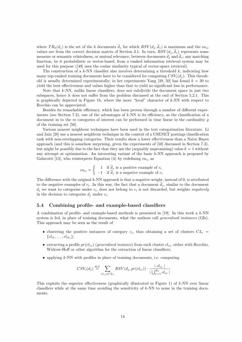
The Rocchio classifier, as all linear classifiers, has the disadvantage that it basically dividesthe space of documents in two subspaces; any document falling within the former (in the case ofRocchio, an n-sphere) will be classified under ci, while all documents falling within the latter willnot. This situation is graphically depicted in Figure 1a, where documents are classified within ci

if and only if they fall within the circle. Note that even most of the positive training exampleswould not be classified correctly by the classifier. This is clear from the fact that what Rocchiobasically does is taking the average (centroid) of all positive examples, and as all averages this isonly partly representative of the whole set6.

5.3 Example-based classifiers

Example-based classifiers do not build an explicit, declarative representation of the category ofinterest, but “parasite” on the categorisation judgments that the experts have given on the trainingdocuments similar to the one to be categorised. These classifiers have thus been called lazy learningsystems, since they do not involve a true training phase [50].

The first introduction of example-based methods in the text classification literature is due toMasand et al. [7, 30]. Our presentation of the example-based approach will be based instead on thek-NN (for “k nearest neighbours”) algorithm implemented by Yang in the ExpNet system [49]. Fordeciding whether dj should be classified under ci, k-NN looks at whether the k training documentsmost similar to dj have also been classified under ci; if the answer is positive for a large enoughproportion of them, a positive categorisation decision is taken, and a negative decision is takenotherwise.

Mathematically, classifying a document by means of k-NN comes down to computing

CSVi(dj) =∑

dz∈ TRk(dj)

RSV (dj , dz) · caiz (4)

6The subdivision into different clusters of the positive training examples which is depicted in Figure 1a is quiteplausible. This could be the case, for example, of a news categorisation task, and of a set of positive trainingexamples for the category Sports; one of the clusters could consist of articles about basketball and another aboutskiing, with the former ones having little in common with the latter ones.

13

where TRk(dj) is the set of the k documents dz for which RSV (dj , dz) is maximum and the caiz

values are from the correct decision matrix of Section 3.1. In turn, RSV (dj , dz) represents somemeasure or semantic relatedness, or mutual relevance, between documents dj and dz; any matchingfunction, be it probabilistic or vector-based, from a ranked information retrieval system may beused for this purpose ([49] uses the cosine similarity typical of vector-space retrieval).

The construction of a k-NN classifier also involves determining a threshold k, indicating howmany top-ranked training documents have to be considered for computing CSVi(dj). This thresh-old is usually determined experimentally; in her experiments Yang [49, 50] has found k = 30 toyield the best effectiveness and values higher than that to yield no significant loss in performance.

Note that k-NN, unlike linear classifiers, does not subdivide the document space in just twosubspaces, hence it does not suffer from the problem discussed at the end of Section 5.2.1. Thisis graphically depicted in Figure 1b, where the more “local” character of k-NN with respect toRocchio can be appreciated.

Besides its remarkable efficiency, which has been proven through a number of different exper-iments (see Section 7.3), one of the advantages of k-NN is its efficiency, as the classification of adocument in to the m categories of interest can be performed in time linear in the cardinality gof the training set [50].

Various nearest neighbour techniques have been used in the text categorisation literature. Liand Jain [28] use a nearest neighbour technique in the context of a USENET postings classificationtask with non-overlapping categories. Their results show a lower effectiveness than a Naive Bayesapproach (and this is somehow surprising, given the experiments of [50] discussed in Section 7.3),but might be possibly due to the fact that they use the (arguably unpromising) value k = 1 withoutany attempt at optimisation. An interesting variant of the basic k-NN approach is proposed byGalavotti [13], who reinterprets Equation (4) by redefining caiz as

caiz ={

1 if dz is a positive example of ci

−1 if dz is a negative example of ci

The difference with the original k-NN approach is that a negative weight, instead of 0, is attributedto the negative examples of ci. In this way, the fact that a document dz, similar to the documentdj we want to categorise under ci, does not belong to ci is not discarded, but weights negativelyin the decision to categorise dj under ci.

5.4 Combining profile- and example-based classifiers

A combination of profile- and example-based methods is presented in [19]. In this work a k-NNsystem is fed, in place of training documents, what the authors call generalised instances (GIs).This approach may be seen as the result of

• clustering the positive instances of category ci, thus obtaining a set of clusters CLi ={cli1, . . . , cliki};

• extracting a profile pr(cliz) (generalised instance) from each cluster cliz, either with Rocchio,Widrow-Hoff or other algorithm for the extraction of linear classifiers;

• applying k-NN with profiles in place of training documents, i.e. computing

CSVi(dj)def=

∑cliz∈CLi

RSV (dj , pr(cliz)) ·| cliz |

| ⋃iki

v=1 cliv |

This exploits the superior effectiveness (graphically illustrated in Figure 1) of k-NN over linearclassifiers while at the same time avoiding the sensitivity of k-NN to noise in the training docu-ments.

14

Categorisation behaviour for k-NN like classifiersCategorisation behaviour for linear classifiers

Negative training examples

Positive training examples

Influence area of the classifier

Figure 1: The categorisation behaviour of linear and non-linear classifiers.

5.5 Classifier committees

The method of classifier committees (or ensembles) is based on the idea that, given a task thatrequires expert knowledge to be performed, k experts may be better than one if their individualjudgments are appropriately combined. In text classification, the idea is to apply k differentclassifiers {Φ1, . . . , Φk} to the same task of deciding whether document dj should be classifiedunder category ci, and then combine their outcome appropriately. Such a classifier committee isthen characterised by i) a choice of k classifiers, and ii) a choice of a combination function.

Concerning the former issue, it is well-known from the machine learning literature that, in orderto guarantee good effectiveness, the classifiers forming the committee should be as independent aspossible, i.e. should be possibly based on radically different intuitions on how classification is to beperformed. The classifiers may be different in terms of the indexing approach followed, or in termsof the inductive method applied in order to induce them, or both. Within text classification, theonly avenue which has been explored is, to our knowledge, the second.

Different combination rules have been experimented with in the literature. The simplest pos-sible rule is majority voting (MV), whereby the binary classification judgments obtained by thek classifiers are pooled together, and the classification decision that reaches the majority of k+1

2votes is taken (k obviously needs to be an odd number) [28]. This method is particularly suitedto the case in which the committee includes classifiers characterised by a binary decision functionCSVi : D → {0, 1}. Another possible policy is dynamic classifier selection (DCS), whereby amongcommittee {Φ1, . . . , Φk} the classifier Φt that yields the best effectiveness on the l validationexamples most similar to dj is selected, and his judgment adopted by the committee [28]. Astill different policy, somehow intermediate between MV and DCS, is adaptive classifier combina-tion (ACC), whereby the judgments of all the classifiers in the committee are summed together,but their individual contribution is weighted by the effectiveness that they have shown on the lvalidation examples most similar to dj [28].

Classifier committees have had mixed results in text categorisation so far. Li and Jain [28]have experimented with a committee formed of (various combinations of) a Naive Bayes classifier,a nearest neighbour classifier, a decision tree classifier, and a classifier induced by means of theirown “subspace method”; the combination rules they have worked with are MV, DCS and ACC.Only in the case of a committee formed by Naive Bayes and the subspace classifier combined by

15

means of ACC the committee has outperformed, and by a narrow margin, the best individualclassifier (for every attempted classifier combination, anyway, ACC gave better results than MVand DCS). This seems discouraging, especially in the light of the fact that the committee approachis computationally expensive (its cost trivially amounts to the sum of the computational costs ofthe individual classifiers plus the cost incurred for the computation of the combination rule). Ithas to be remarked, however, that the small size of their experiment (two test sets of less than700 documents each were used) does not allow to draw definitive conclusions on the approachesadopted.

6 Determining thresholds

There are various possible policies for determining the threshold τi discussed at the beginning ofSection 5, also depending on the constraints imposed by the application.

One possible policy is CSV thresholding (also called probability thresholding in the case ofprobabilistic classifiers [21], or Scut [50]) [46]. In this case the threshold τi is a value of theCSVi function. Lewis [21] considered using a fixed threshold τ equal for all ci’s, but notedthat this might result in assigning all the test docs to category ci while not even assigning asingle test document to category cj . He then considered using different thresholds τi for differentcategories ci established by normalising probability estimates (following a suggestion from [29]).His experimental results did not show, however, a considerable difference in effectiveness betweenthe two variants. Yang [50] uses different thresholds τi for the different categories ci. Eachthreshold is optimised by testing different values for it on the validation set and choosing thevalue which yields the best value of the chosen effectiveness function.

A second, popular policy is proportional thresholding [21, 46] (also called Pcut in [50]). Theaim of this policy is to set the threshold τi so that the test set generality gTe(ci) of a category ci

is as close as possible to its training set generality gTr(ci). This idea encodes the quite sensibleprinciple according to which both in training set and test set the same percentage of documents ofthe original set should be classified under ci. One drawback of this thresholding policy is that, forobvious reasons, it does not lend itself to document-pivoted categorisation. Yang [50] proposes astill more refined version of this policy, i.e. one in which a factor x (equal for all ci’s) is multipliedto gTr(ci) to actually obtain gTe(ci). Yang claims that this factor, whose value is to be empiricallydetermined by experimentation on a validation set, allows a smoother trade-off between recall andprecision to be obtained (see Section 7.1.1). For both k-NN and LLSF she found that optimalvalues lie in the [1.2, 1.3] range.

Sometimes, depending on the application, a fixed thresholding policy (also known as “k-per-doc” thresholding [21] or Rcut [50]) is applied, whereby it is stipulated that a fixed number k ofcategories, equal for all dj ’s, are to be assigned to each document dj . Strictly speaking, however,this is not a thresholding policy in the sense defined at the beginning of Section 5, as it mighthappen that d′ is categorised under ci, d′′ is not, and CSVi(d′) < CSVi(d′′). Quite clearly, thispolicy is mostly at home with document-pivoted categorisation. It suffers, however, from a certaincoarseness, as the fact that k is equal for all documents (nor could this be otherwise) does notallow system fine-tuning.

In terms of experimental results, Lewis [21] found the proportional policy to be definitelysuperior to CSV thresholding when microaveraged effectiveness was tested but slightly inferiorwhen using macroaveraging (see Section 7.1.1). Yang [50] found instead CSV thresholding tobe superior to proportional thresholding (possibly due to her category-specific optimisation on avalidation set), and found fixed thresholding to be consistently inferior to the other two policies.Of course, the fact that these results have been obtained across different classifiers no doubtreinforce them. In general, aside from the considerations above, the choice of the thresholdingpolicy may also be influenced by the application; for instance, in applying a text classifier todocument indexing for Boolean systems, a fixed thresholding policy might be chosen, while aproportional or CSV thresholding method might be chosen for Web page classification underYahoo!-like catalogues.

16

7 Evaluation issues for document categorisation

As in the case of information retrieval systems, the evaluation of document classifiers is typicallyconducted experimentally, rather than analytically. The reason for this tendency is that, in orderto evaluate a system analytically (e.g. proving that the system is correct and complete) we alwaysneed a formal specification of the problem that the system is trying to solve (e.g. with respectto what correctness and completeness are defined), and the central notion of document classifica-tion (namely, that of relevance of a document to a category) is, due to its subjective character,inherently non-formalisable.

The experimental evaluation of classifiers, rather than concentrating on issues of efficiency,usually tries to evaluate the effectiveness of a classifier, i.e. its capability of taking the rightcategorisation decisions. The main reasons for this bias are that:

• efficiency is a notion dependent on the hw/sw technology used. Once this technology evolves,the results of experiments aimed at establishing efficiency are no longer valid. This doesnot happen for effectiveness, as any experiment aimed at measuring effectiveness can bereplicated, with identical results, on any different or future hw/sw platform;

• effectiveness is really a measure of how the system is good at tackling the central notion ofclassification, that of relevance of a document to a category.

7.1 Measures of categorisation effectiveness

7.1.1 Precision and recall

Classification effectiveness is measured in terms of the classic IR notions of precision (Pr) andrecall (Re), adapted to the case of document categorisation. Precision wrt ci (Pri) is defined asthe conditional probability P (caix = 1 | aix = 1), i.e. as the probability that if a random documentdx is categorised under ci, this decision is correct. Analogously, recall wrt ci (Rei) is defined as theconditional probability P (aix = 1 | caix = 1), i.e. as the probability that, if a random documentdx should be categorised under ci, this decision is taken. These category-relative values may beaveraged, in a way to be discussed shortly, to obtain Pr and Re, i.e. values global to the wholecategory set. Borrowing terminology from logic, Pr may be viewed as the “degree of soundness” ofthe classifier wrt the given category set C, while Re may be viewed as its “degree of completeness”wrt C.

As they are defined here, Pri and Rei (and consequently Pr and Re) are to be understood,in the line of [48], as subjective probabilities, i.e. values measuring the expectation of the userthat the system will behave correctly when classifying a random document under ci. Theseprobabilities may be estimated in terms of the contingency table for category ci on a given test set(see Table 2). Here, FPi (false positives wrt ci) is the number of documents of the test set thathave been incorrectly classified under ci; TNi (true negatives wrt ci), TPi (true positives wrt ci)and FNi (false negatives wrt ci) are defined accordingly. Precision wrt ci and recall wrt ci maythus be estimated as

Priest=

TPi

TPi + FPi(5)

Reiest=

TPi

TPi + FNi(6)

For obtaining estimates of precision and recall relative to the whole category set, two differentmethods may be adopted:

• microaveraging: precision and recall are obtained by globally summing over all individualdecisions, i.e.:

Prµ est=TP

TP + FP(7)

17

Category expert judgmentsci YES NO

classifier YES TPi FPi

judgments NO FNi TNi

Table 2: The contingency table for category ci.

Category set expert judgmentsC = {c1, . . . , cm} YES NO

classifier YES TP =m∑

i=1

TPi FP =m∑

i=1

FPi

judgments NO FN =m∑

i=1

FNi TN =m∑

i=1

TNi

Table 3: The global contingency table.

Reµ est=TP

TP + FN=

∑mi=1 TPi∑m

i=1(TPi + FNi)(8)

where the “µ” superscript stands for microaveraging. For this, the “global” contingency tableof Table 3, obtained by summing over all category-specific contingency tables, is needed.

• macroaveraging : precision and recall are first evaluated “locally” for each category, andthen “globally” by averaging over the results of the different categories, i.e.:

PrM est=∑m

i=1 Pri

m(9)

ReM est=∑m

i=1 Rei

m(10)

where the “M” superscript stands for macroaveraging.

It is important to recognise that these two methods may give quite different results, especiallyif the different categories are unevenly populated: for instance, if the classifier performs well oncategories with a small number of positive test instances, its effectiveness will probably be betteraccording to macroaveraging than according to microaveraging. There is no agreement amongauthors on which is better. Some believe that “microaveraged performance is somewhat misleading(. . . ) because more frequent topics are weighted heavier in the average” [46, page 327] andthus favour macroaveraging, while others believe that topics should indeed count proportionallyto their frequence, and thus lean towards microaveraging. From now on, we will assume thatmicroaveraging is used, and will thus drop the “i” subscript from Pr, Re and other symbols; itshould be clear, however, that everything we will say in the rest of Section 7 may be adapted tothe case of macroaveraging in the obvious way.

7.1.2 Combined measures

Neither precision nor recall make sense in isolation of the other. In fact, in order to obtain aclassifier with 100% recall, one would only need to set every threshold τi to 0, thereby obtainingthe trivial acceptor (i.e. the classifier that sets aij = 1 for all 1 ≤ i ≤ m, 1 ≤ j ≤ n, i.e. thatclassifies all documents under all categories). Quite obviously, in this case precision would usuallybe very low (more precisely, equal to apc, the average percentage of categories per test document).

18

Conversely, it is well-known from everyday information retrieval practice that higher levels ofprecision may be obtained at the price of a low recall.

In practice, by tuning thresholds τi a classification algorithm is tuned so as to improve Pr tothe detriment of Re or viceversa. A classifier should thus be measured by means of a “combined”effectiveness measure which both Pr and Re concur to determine. Various such measures havebeen proposed, among which the following are most frequent:

• effectiveness is computed as (interpolated) 11-point average precision. That is, each thresholdτi is successively set to the values for which recall takes up values of 0.0, 0.1, . . . , 0.9, 1.0;for these 11 different thresholds precision is computed and averaged over the 11 resultingvalues. This methodology is completely analogous to the standard evaluation methodologyfor IR systems, and may be used

– with categories being used in place of queries. This is most frequently used in the caseof document-pivoted categorisation (see e.g [43, 49, 50, 53]);

– with documents being used in place of queries and categories in place of documents.This is most frequently used in the case of category-pivoted categorisation (see e.g. [46,Section 6.1]. Note that in this case if macroaveraging is used, it needs to be redefinedon a per-document, rather than per-category, basis.

• effectiveness is computed as the breakeven point, i.e. the value at which Pr equals Re (e.g. [1,21, 26]). In all reasonable classifiers a value for each τi for which Pr and Re are (almost)equal does exist, since by increasing τi from 0 to 1 Pr increases monotonically and Redecreases monotonically. If for no value of τi Pr and Re are exactly equal, τi is set to thevalue for which Pr and Re are closest, and an interpolated breakeven is computed as theaverage of the the values of Pr and Re. As noted in [50], when for no value of τi Pr and Reare close enough, interpolated breakeven may not be a reliable indicator of the effectivenessof the classifier;

• effectiveness is computed as the value of the Fα function, for some 0 ≤ α ≤ 1 (e.g. [23]), i.e.

Fα =1

α1Pr

+ (1 − α)1Re

In this formula α may be seen as the relative degree of importance attributed to Pr and Re:if α = 1, then Fα coincides with Pr, if α = 0 then Fα coincides with Re. Usually, a valueof α = 0.5 is used, which attributes equal importance to Pr and Re; for reasons we do notwant to enter here, rather than F0.5 this is usually called called F1 (see [23] for details). Asshown in [50], for a given classifier Φ, its breakeven value is always less or equal than its F1

value.

Once an effectiveness measure is chosen, a classifier can be tuned (e.g. thresholds and other internalparameters can be set) so that the resulting effectiveness is the best achievable by that classifier.The tuning of a parameter p (be it a threshold or other) is normally done experimentally. Thismeans performing repeated experiments on the validation set in the same experimental conditions,with the values of the other parameters pk fixed (at a default value, in the case of a yet-to-be-tuned parameter pk, or at the chosen value, if the parameter pk has already been tuned) and withdifferent values for parameter p. At the end of the process, the value that has yielded the besteffectiveness is chosen for p.

7.2 Test collections

For experimentation purposes, standard test collections (playing a role akin to the test collectionsof IR) are available in the public domain. Typical examples include

19

• the Reuters-21578 corpus, consisting of a revised version of an older corpus known asReuters-22173 [22]. The documents are newswire stories covering the period between1987 and 1991;

• the Ohsumed corpus [16]. The documents are titles or title-plus-abstract’s from medicaljournals (Ohsumed actually consists of a subset of the Medline document base); the cat-egories are the postable terms of the Mesh thesaurus [35].

These two test collections (especially Reuters-21578 together with its older version) accountfor most of the experimentation that has been performed to date in text categorisation. Unfor-tunately, this does not mean that we have definitive results concerning how well a given classifiercompares to another, in the sense that many of these experiments have been carried out in some-times subtly different experimental conditions. In fact, at least six different versions (includingReuters-21578) of the Reuters-22173 collection have been carved out of the original and usedfor experimentation.

In order for the experimental results on two different classifiers to be directly comparable, theexperiments should be performed under the following conditions:

1. the same collection (i.e. same documents and same categories) is used for both classifiers;

2. the same choice (“split”) of training set and test set is made for both classifiers;

3. the same effectiveness measure is used for both classifiers.

Unfortunately, much of earlier experimentation (at least until 1997) was not performed with thiscaveat in mind, which means that the results reported by these researches are seldom directlycomparable. By experimenting three different classifiers on five versions of Reuters-22173,Yang [52] has experimentally shown that a lack of compliance with these three conditions (andwith Condition 1 in particular) may significantly influence the experimental results. In particular,[52] shows that experiments carried out on Version 2 are not directly comparable with thoseusing later versions, since the former includes a significant percentage (58%) of “unlabelled” testdocuments which, being negative examples of all categories, tend to depress effectiveness. Manyof these documents appear to have simply not been considered by the human categorisers, ratherthan having consciously been deemed not to belong to any category; Version 2 is thus simply nota good testbed for automatic classifiers.

7.3 Which classifier is best?

In what may be regarded as the first large-scale cross-experimental evaluation in the text cate-gorisation literature, Yang [52] has been able to obtain indications on the relative performance ofthe various methods described in the literature. This was achieved by using either

• direct comparison: classifiers C ′ and C ′′ are experimented on the same test collection TCby using a common evaluation measure;

• indirect comparison:

1. classifier C ′ is tested on test collection TC ′ and classifier C ′′ is tested on test collectionTC ′′;

2. one or more “baseline” classifiers C1, . . . , Cm are tested on both TC ′ and TC ′′.

Test 2 can give an indication of the relative “hardness” of the two collections; using boththis indication and the results from Test 1 yields an indication on the relative value of thetwo classifiers.

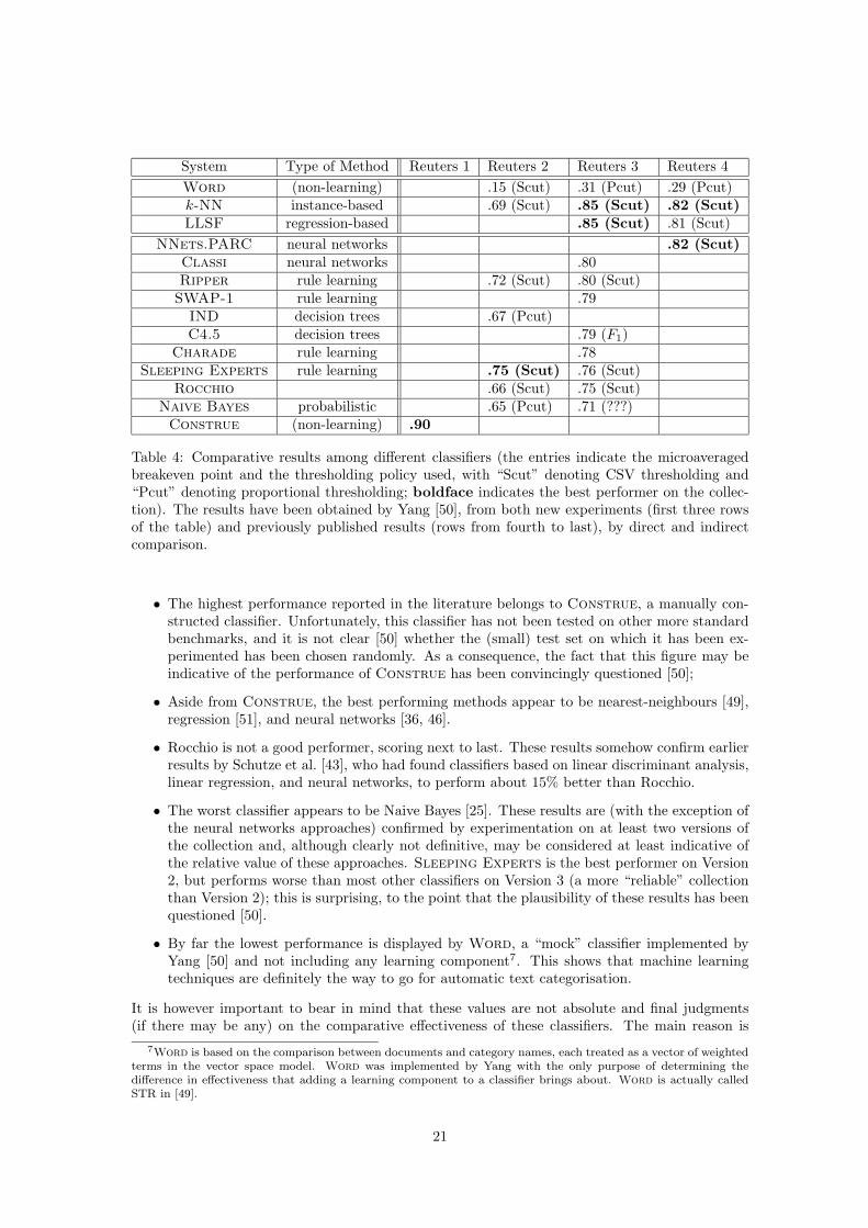
The results reported in this evaluation are illustrated in Table 4. A number of interesting conclu-sions can be drawn from them (for more detailed discussions on these results see [50]):

20

System Type of Method Reuters 1 Reuters 2 Reuters 3 Reuters 4Word (non-learning) .15 (Scut) .31 (Pcut) .29 (Pcut)k-NN instance-based .69 (Scut) .85 (Scut) .82 (Scut)LLSF regression-based .85 (Scut) .81 (Scut)

NNets.PARC neural networks .82 (Scut)Classi neural networks .80Ripper rule learning .72 (Scut) .80 (Scut)SWAP-1 rule learning .79

IND decision trees .67 (Pcut)C4.5 decision trees .79 (F1)

Charade rule learning .78Sleeping Experts rule learning .75 (Scut) .76 (Scut)

Rocchio .66 (Scut) .75 (Scut)Naive Bayes probabilistic .65 (Pcut) .71 (???)Construe (non-learning) .90

Table 4: Comparative results among different classifiers (the entries indicate the microaveragedbreakeven point and the thresholding policy used, with “Scut” denoting CSV thresholding and“Pcut” denoting proportional thresholding; boldface indicates the best performer on the collec-tion). The results have been obtained by Yang [50], from both new experiments (first three rowsof the table) and previously published results (rows from fourth to last), by direct and indirectcomparison.

• The highest performance reported in the literature belongs to Construe, a manually con-structed classifier. Unfortunately, this classifier has not been tested on other more standardbenchmarks, and it is not clear [50] whether the (small) test set on which it has been ex-perimented has been chosen randomly. As a consequence, the fact that this figure may beindicative of the performance of Construe has been convincingly questioned [50];

• Aside from Construe, the best performing methods appear to be nearest-neighbours [49],regression [51], and neural networks [36, 46].

• Rocchio is not a good performer, scoring next to last. These results somehow confirm earlierresults by Schutze et al. [43], who had found classifiers based on linear discriminant analysis,linear regression, and neural networks, to perform about 15% better than Rocchio.

• The worst classifier appears to be Naive Bayes [25]. These results are (with the exception ofthe neural networks approaches) confirmed by experimentation on at least two versions ofthe collection and, although clearly not definitive, may be considered at least indicative ofthe relative value of these approaches. Sleeping Experts is the best performer on Version2, but performs worse than most other classifiers on Version 3 (a more “reliable” collectionthan Version 2); this is surprising, to the point that the plausibility of these results has beenquestioned [50].

• By far the lowest performance is displayed by Word, a “mock” classifier implemented byYang [50] and not including any learning component7. This shows that machine learningtechniques are definitely the way to go for automatic text categorisation.

It is however important to bear in mind that these values are not absolute and final judgments(if there may be any) on the comparative effectiveness of these classifiers. The main reason is

7Word is based on the comparison between documents and category names, each treated as a vector of weightedterms in the vector space model. Word was implemented by Yang with the only purpose of determining thedifference in effectiveness that adding a learning component to a classifier brings about. Word is actually calledSTR in [49].

21

that comparisons tend to be pretty reliable when they concern new experiments, performed byone author under carefully controlled conditions. However, they are more problematic when theyinvolve different classifiers tested as part of different experiments, which is very much the casewhen comparing results published by different people. As pointed out in [50], in this case variousfactors, often extraneous to the learning algorithm proper, may have influenced the experimentalresults. This may include, among others, different choices in pre-processing (stemming, etc.)and indexing, or different standards of compliance with safe scientific practice (such as tuningparameters on the test set rather than on a separate validation set), which often are not detailedin published papers. One can only subscribe to the common belief that more experimentation ontruly common benchmarks needed in order to arrive at more definitive conclusions.

References

[1] C. Apte, F. Damerau, and S. Weiss. Automated learning of decision rules for text categoriza-tion. ACM Transactions on Information Systems, 12(3):233–251, 1994.

[2] G. Attardi, A. Gullı, and F. Sebastiani. Automatic Web page categorization by link and con-text analysis. In C. Hutchison and G. Lanzarone, editors, Proceedings of THAI’99, EuropeanSymposium on Telematics, Hypermedia and Artificial Intelligence, pages 105–119, Varese, IT,1999.

[3] N. J. Belkin and W. B. Croft. Information filtering and information retrieval: two sides ofthe same coin? Communications of the ACM, 35(12):29–38, 1992.

[4] P. Biebricher, N. Fuhr, G. Lustig, and M. Schwantner. The automatic indexing systemAIR/PHYS. From research to application. In Proceedings of SIGIR-88, 11th ACM Inter-national Conference on Research and Development in Information Retrieval, pages 333–342,Grenoble, FR, 1988. Also reprinted in [45], pp. 513–517.

[5] C. Cleverdon. Optimizing convenient online access to bibliographic databases. InformationServices and Use, 4(1):37–47, 1984. Also reprinted in [47], pp. 32–41.

[6] W. W. Cohen and Y. Singer. Context-sensitive learning for text categorization. In Pro-ceedings of SIGIR-96, 19th ACM International Conference on Research and Development inInformation Retrieval, pages 307–315, Zurich, CH, 1996.

[7] R. M. Creecy, B. M. Masand, S. J. Smith, and D. L. Waltz. Trading MIPS and memory forknowledge engineering: classifying census returns on the Connection Machine. Communica-tions of the ACM, 35(8):48–63, 1992.

[8] S. Deerwester, S. T. Dumais, G. W. Furnas, T. K. Landauer, and R. Harshman. Indexing bylatent semantic indexing. Journal of the American Society for Information Science, 41(6):391–407, 1990.

[9] J. L. Fagan. Experiments in automatic phrase indexing for document retrieval: a comparisonof syntactic and non-syntactic methods. PhD thesis, Department of Computer Science, CornellUniversity, Ithaca, US, 1987.

[10] B. Field. Towards automatic indexing: automatic assignment of controlled-language indexingand classification from free indexing. Journal of Documentation, 31(4):246–265, 1975.

[11] N. Fuhr, N. Govert, M. Lalmas, and F. Sebastiani. Categorisation tool: Final prototype.Deliverable 4.3, TELEMATICS Project LE4-8303 “EUROSEARCH”, Commission of the Eu-ropean Communities, 1999.

22

[12] N. Fuhr, S. Hartmann, G. Knorz, G. Lustig, M. Schwantner, and K. Tzeras. AIR/X – arule-based multistage indexing system for large subject fields. In Proceedings of RIAO’91,3rd International Conference “Recherche d’Information Assistee par Ordinateur”, pages 606–623, Barcelona, ES, 1991.

[13] L. Galavotti. Un sistema modulare per la classificazione di testi basato sull’apprendimentoautomatico. Master’s thesis, Dipartimento di Informatica, Universita di Pisa, Pisa, IT, 1999.

[14] W. A. Gale, K. W. Church, and D. Yarowsky. A method for disambiguating word senses ina large corpus. Computers and the Humanities, 26(5):415–439, 1993.

[15] P. J. Hayes and S. P. Weinstein. CONSTRUE/TIS: a system for content-based indexingof a database of news stories. In Proceedings of IAAI-90, 2nd Conference on InnovativeApplications of Artificial Intelligence, pages 1–5, 1990.

[16] W. Hersh, C. Buckley, T. Leone, and D. Hickman. Ohsumed: an interactive retrieval eval-uation and new large text collection for research. In Proceedings of SIGIR-94, 17th ACMInternational Conference on Research and Development in Information Retrieval, pages 192–201, Dublin, IE, 1994.

[17] D. A. Hull. Improving text retrieval for the routing problem using latent semantic indexing. InProceedings of SIGIR-94, 17th ACM International Conference on Research and Developmentin Information Retrieval, pages 282–289, Dublin, IE, 1994.

[18] D. J. Ittner, D. D. Lewis, and D. D. Ahn. Text categorization of low quality images. InProceedings of SDAIR-95, 4th Annual Symposium on Document Analysis and InformationRetrieval, pages 301–315, Las Vegas, US, 1995.

[19] W. Lam and C. Y. Ho. Using a generalized instance set for automatic text categorization. InProceedings of SIGIR-98, 21st ACM International Conference on Research and Developmentin Information Retrieval, pages 81–89, Melbourne, AU, 1998.

[20] M. E. Lesk. Automatic word sense disambiguation: how to tell a pine cone from an ice creamcone. In V. DeBuys, editor, Proceedings of SIGDOC-86, 5th ACM International Conferenceon Systems Documentation, pages 24–26, New York, US, 1986.

[21] D. D. Lewis. An evaluation of phrasal and clustered representations on a text categorizationtask. In Proceedings of SIGIR-92, 15th ACM International Conference on Research andDevelopment in Information Retrieval, pages 37–50, Kobenhavn, DK, 1992.

[22] D. D. Lewis. Representation and learning in information retrieval. PhD thesis, Departmentof Computer Science, University of Massachusetts, Amherst, US, 1992.

[23] D. D. Lewis. Evaluating and optmizing autonomous text classification systems. In Pro-ceedings of SIGIR-95, 18th ACM International Conference on Research and Development inInformation Retrieval, pages 246–254, Seattle, US, 1995.

[24] D. D. Lewis. Naive (Bayes) at forty: The independence assumption in information retrieval.In Proceedings of ECML-98, 10th European Conference on Machine Learning, pages 4–15,Chemnitz, DE, 1998.

[25] D. D. Lewis and W. A. Gale. A sequential algorithm for training text classifiers. In Pro-ceedings of SIGIR-94, 17th ACM International Conference on Research and Development inInformation Retrieval, pages 3–12, Dublin, IE, 1994.

[26] D. D. Lewis and M. Ringuette. A comparison of two learning algorithms for text catego-rization. In Proceedings of SDAIR-94, 3rd Annual Symposium on Document Analysis andInformation Retrieval, pages 81–93, Las Vegas, US, 1994.

23

[27] D. D. Lewis, R. E. Schapire, J. P. Callan, and R. Papka. Training algorithms for linear textclassifiers. In Proceedings of SIGIR-96, 19th ACM International Conference on Research andDevelopment in Information Retrieval, pages 298–306, Zurich, CH, 1996.

[28] Y. H. Li and A. K. Jain. Classification of text documents. The Computer Journal, 41(8):537–546, 1998.

[29] M. Maron. Automatic indexing: an experimental inquiry. Journal of the Association forComputing Machinery, 8(3):404–417, 1961.

[30] B. Masand, G. Linoff, and D. Waltz. Classifying news stories using memory-based reasoning.In Proceedings of SIGIR-92, 15th ACM International Conference on Research and Develop-ment in Information Retrieval, pages 59–65, Kobenhavn, DK, 1992.

[31] T. Mitchell. Machine learning. McGraw Hill, New York, US, 1996.

[32] D. Mladenic. Turning Yahoo! into an automatic Web page classifier. In Proceedings ofECAI’98, 13th European Conference on Artificial Intelligence, pages 473–474, Brighton, UK,1998.

[33] D. Mladenic and M. Grobelnik. Feature selection for classification based on text hierarchy.In Proceedings of the Workshop on Learning from Text and the Web, Pittsburgh, USA, 1998.

[34] National Aeronautics and Space Administration, Washington, US. NASA thesaurus, 1994edition. Accessible at http://www.sti.nasa.gov/nasa-thesaurus.html.

[35] National Library of Medicine, Bethesda, US. Medical Subject Headings (MeSH), 1993 edition.

[36] H. T. Ng, W. B. Goh, and K. L. Low. Feature selection, perceptron learning, and a usabilitycase study for text categorization. In Proceedings of SIGIR-97, 20th ACM International Con-ference on Research and Development in Information Retrieval, pages 67–73, Philadelphia,US, 1997.

[37] H. Ragas and C. H. Koster. Four text classification algorithms compared on a Dutch corpus. InProceedings of SIGIR-98, 21st ACM International Conference on Research and Developmentin Information Retrieval, pages 369–370, Melbourne, AU, 1998.

[38] S. E. Robertson and K. Sparck Jones. Relevance weighting of search terms. Journal of theAmerican Society for Information Science, 27(3):129–146, 1976. Also reprinted in [47], pp.143–160.

[39] G. Salton and C. Buckley. Term-weighting approaches in automatic text retrieval. InformationProcessing and Management, 24(5):513–523, 1988. Also reprinted in [45], pp. 323–328.

[40] G. Salton, A. Wong, and C. Yang. A vector space model for automatic indexing. Communi-cations of the ACM, 18(11):613–620, 1975. Also reprinted in [45], pp. 273–280.

[41] T. Saracevic. Relevance: a review of and a framework for the thinking on the notion ininformation science. Journal of the American Society for Information Science, 26(6):321–343, 1975. Also reprinted in [45], pp. 143–165.

[42] H. Schutze. Automatic word sense discrimination. Computational Linguistics, 24(1):97–124,1998.

[43] H. Schutze, D. A. Hull, and J. O. Pedersen. A comparison of classifiers and documentrepresentations for the routing problem. In Proceedings of SIGIR-95, 18th ACM InternationalConference on Research and Development in Information Retrieval, pages 229–237, Seattle,US, 1995.

24

[44] A. F. Smeaton. Using NLP or NLP resources for information retrieval tasks. In T. Strza-lkowski, editor, Natural language information retrieval. Kluwer Academic Publishers, Dor-drecht, NL, 1997.

[45] K. Sparck Jones and P. Willett, editors. Readings in information retrieval. Morgan Kaufmann,San Mateo, US, 1997.

[46] E. Wiener, J. O. Pedersen, and A. S. Weigend. A neural network approache to topic spotting.In Proceedings of SDAIR-95, 4th Annual Symposium on Document Analysis and InformationRetrieval, pages 317–332, Las Vegas, US, 1995.

[47] P. Willett, editor. Document retrieval systems. Taylor Graham, London, UK, 1988.

[48] S. M. Wong and Y. Yao. On modeling information retrieval with probabilistic inference. ACMTransactions on Information Systems, 13(1):38–68, 1995.

[49] Y. Yang. Expert network: effective and efficient learning from human decisions in textcategorisation and retrieval. In Proceedings of SIGIR-94, 17th ACM International Conferenceon Research and Development in Information Retrieval, pages 13–22, Dublin, IE, 1994.

[50] Y. Yang. An evaluation of statistical approaches to text categorization. Information retrieval,1-2(1):69–90, 1999.

[51] Y. Yang and C. G. Chute. An example-based mapping method for text categorization andretrieval. ACM Transactions on Information Systems, 12(3):252–277, 1994.

[52] Y. Yang and X. Liu. A re-examination of text categorization methods. In Proceedings ofSIGIR-99, 22nd ACM International Conference on Research and Development in InformationRetrieval, Berkeley, US, 1999. Forthcoming.

[53] Y. Yang and J. O. Pedersen. A comparative study on feature selection in text categorization.In Proceedings of ICML-97, 14th International Conference on Machine Learning, pages 412–420, Nashville, US, 1997.

25