Knowledge and Information Systems (2021) 63:2693–2718https://doi.org/10.1007/s10115-021-01602-3

REGULAR PAPER

A turning point prediction method of stock price basedon RVFL-GMDH and chaotic time series analysis

Junde Chen1 · Shuangyuan Yang1 · Defu Zhang1 · Y. A. Nanehkaran1

Received: 11 May 2020 / Revised: 18 July 2021 / Accepted: 24 July 2021 / Published online: 26 August 2021© The Author(s), under exclusive licence to Springer-Verlag London Ltd., part of Springer Nature 2021

AbstractStock market prediction is extremely important for investors because knowing the futuretrend of stock prices will reduce the risk of investing capital for profit. Therefore, seekingan accurate, fast, and effective approach to identify the stock market movement is of greatpractical significance. This study proposes a novel turning point prediction method for thetime series analysis of stock price. Through the chaos theory analysis and application, we putforward a new modeling approach for the nonlinear dynamic system. The turning indicatorof time series is computed firstly; then, by applying the RVFL-GMDH model, we performthe turning point prediction of the stock price, which is based on the fractal characteristic of astrange attractor with an infinite self-similar structure. The experimental findings confirm theefficacy of the proposed procedure and have become successful for the intelligent decisionsupport of the stock trading strategy.

Keywords Turning point prediction · Chaotic time series · Phase space reconstruction ·RVFL-GMDH · Stock market

1 Introduction

The stock market is a complicated and varied system due to the chaotic, blaring, and non-stationary data. The fast and accurate prediction of the stock market becomes challengingamong the investors to invest the capital for making profits. Therefore, plenty of previousresearch has been done in this field, and they can be generally summarized in two categories:linear models based on statistical theories; and nonlinear models based on machine learning

B Defu Zhangdfzhang@xmu.edu.cn

Junde Chen23020180155666@stu.xmu.edu.cn

Shuangyuan Yangyangshuangyuan@xmu.edu.cn

Y. A. Nanehkaranartavil20@gmail.com

1 School of Informatics, Xiamen University, Xiamen 361005, China

123

2694 J. Chen et al.

[1, 2]. In the existing methods of statistical models, time series [3], gray [4], vector autore-gression (VAR) [5], and others are usually used. These prediction methods such as linearregression, moving average, and GARCH are much favorable for financial time series fore-casting because of their interpretability [6]. They perform well in linear and stationary timeseries while do not accomplish ideally on the nonlinear and non-stationary data.

Apart from the traditional statistical methods, data mining and machine learning havecarved their own niches in time series analysis [7, 8]. Regarding data mining studies utilizedin daily stock data, there are prediction works based on the support vector machine (SVM) [9,10]. To determine whether the new pattern data belong to a certain category, artificial neuralnetworks (ANN) [11, 12] has achieved successful predictions even with complicated rela-tionships between variables. The fuzzy time series (FTS) [13, 14] method is also employed topredict and identify the time series variation. Including particle swarm optimization (PSO),genetic algorithm (GA), and rough sets theory (RS), the well-known optimization algorithmshave been used in this field as well. Besides, some other prediction research works are per-formed using the method of word analysis for several news articles [15, 16], etc. In particular,sinceWhite first employed theANN topredict the daily return rate of IBMordinary stock [17],the usage of the ANN in stock price prediction has become a hot research topic [18–20].Morerecently, the deep learning method, and especially convolutional neural networks (CNN), hasshown impressive performance in pattern recognition and classification; it is also employedin forecasting stock price from historical exchange data [21]. For example, Tsantekidis et al.[22] proposed a deep learning methodology, based on Convolutional Neural Networks, topredict the stock prices, and they gained the highest 67.38% precision in 20 prediction hori-zons. Deng et al. [23] trained a recurrent deep neural network (NN) for real-time financialsignal representation and trading; the experimental results on both the stock and the com-modity future markets demonstrated the effectiveness of their proposed approach. Zarkiaset al. [24] reported a novel price trailing approach based on deep reinforcement learning (RL)that went beyond traditional price forecasting, and the experiment conducted on a real datasetdemonstrated their proposed method outperforming a competitive deep RLmethod. Besides,some designed recurrent neural networks (RNNs) have been applied to forecasting the stockdata as well [25, 26]. These studies make full use of the advantages of neural networks suchas self-adapting, self-learning, distributed processing, etc., and overcome the shortcomingsof conventional prediction methods. Nevertheless, there are still problems for these neuralnetwork methods, including low precision, slow convergence, and easy inclination to a localminimum. In addition, a very large number of parameters that need to be trained by a vastamount of labeled data is also a problem for deep neural networks. On the other hand, suchthe price trailing forecast, which is a variant of the price prediction method, does not reallyovercome the limitations of traditional price forecasting influenced by chaos, volatility, andnoise interference. Despite these constraints, the previous studies successfully indicated thepotential of neural network methods in stock forecasting.

As mentioned previously, most of the existing research considered the prediction of pricechanges with the aim of creating accurate models that predict the exact value of a stock priceinstead of the trading strategy itself, such as determining the buy or sell points regarding theknowledge of intelligent stock trading. However, in reality, investors aremore concernedwithmaking trading decisions than forecasting daily prices. So far, there are only a few examplesof research that involve the turning points of a stock, and notably this problem is still alarge one as regards academic researchers and industrial practitioners [1, 11]. Reviewing thelatest literature, we found the following research correlated with the turning point prediction.Tang et al. [27] integrated piecewise linear representation (PLR) and weighted support vectormachine (WSVM) for forecasting stock turning points. Intachai et al. [28] reported a Local

123

A turning point prediction method of stock price based on RVFL-… 2695

Average Model (LAM) to predict the turning points of the stock price. Chang et al. [29]applied an ANN model to learn the connection weights from historical turning points, andafterward, an exponential smoothing based dynamic thresholdmodel was used to forecast thefuture trading signals, etc. The commonly used algorithms including SVM, ANN, and othershave shown the effectiveness in stock turning point prediction. However, as stated earlier,the conventional algorithms such as ANNs exist some disadvantages in avoiding over-fittingand trapping at a local minimum. Thus, referring to the above literature, this paper proposesa RVFL-GMDH based turning point prediction method for the time series analysis of stockprice. Through chaotic time series analysis, the turning signal �(t) of stock price can be gotin advance. Then, the RVFL-GMDH networks, which randomly initializes the weight andbias parameters between the input layer and the hidden layer is employed for the turningpoint prediction of the stock price. A series of experiments are performed and the empiricalanalysis results demonstrate the validity of the proposed procedure.

The rest of this writing is structured in the following hierarchy. Section 2 introduces thechaotic time series analysis and describes the theoretical background. Section 3 discusses themodeling methodology to accomplish the task of turning point prediction along with relatedconcepts and the proposed procedure. Section 4 dedicates to the algorithm experiments;multiple experiments are conducted as well as empirical analysis implemented in practicalapplication scenarios. This paper is ultimately summarized in Sect. 5.

2 Chaotic time series analysis

2.1 Determination of chaotic attractor

Generally, it is easy to get a set of time series values in the economic system, i.e., theone-dimensional information of the system. Although the one-dimensional information con-tains the characteristics of the system, the dynamic or multi-dimensional features of thesystem cannot be reflected by this one-dimensional representation fully, and thus somemulti-dimensional features of the system may be lost. Therefore, Packard proposed to reconstructthe phase space with the delay coordinates of a variable in the original system, and Tak-ens proved that a suitable embedding dimension could be found [30]. It means that if thedimension of the delay coordinate m is greater than or equal to 2d + 1 (m ≥ 2d + 1, d isthe dimension of the dynamic system), the regular trajectory (attractor) can be restored inthe embedding dimension space. Thus, on the orbit of the reconstructed Rm space, the orig-inal dynamic system maintains differential homeomorphism, which lays a solid theoreticalfoundation for the prediction of chaotic time series.

Let the chaotic time series of a single variable be {x(i), i = 1, 2, ..., N }: Then, if theembedding dimension m and time delay τ are selected appropriately, the phase space of thetime series can be expressed in Eq. (1).

(ti ) = [x(ti ), x(ti + τ), x(ti + 2τ), . . . , x(ti + (m − 1)τ )]i = 1, 2, . . . ,m (1)

where τ represents the delay time, m indicates the embedding dimension. Referring to Tak-ens’ theorem, the dynamic characteristics of the attractor can be recovered in the sense oftopological equivalence.

123

2696 J. Chen et al.

A small embedding dimension m0 is first given to form a reconstructed phase space, andthe distance between vectors in phase space can be defined in Eq. (2).

∣∣yi − y j

∣∣ = max

1≤k≤m0

∣∣yik − y jk

∣∣ (2)

The correlation integral of embedded time series is computed by

Cm0(r) = 1

N 2

N∑

i, j=1

θ(r − ∣∣yi − y j

∣∣) (3)

where θ (·) is the Heaviside function, r denotes a certain probability value, and C(r) is acumulative distribution function, representing the probability that the distance in phase spaceis less than r. The function θ (·) is expressed using Eq. (4).

θ(x) ={

0, x ≤ 0

1, x > 0(4)

For an appropriate range of r, the dimension d of attractors and the cumulative distributionfunction C(r) should satisfy the logarithmic linear relationship, as written in Eq. (5).

d(m0) = lnCm0(r)/ ln r (5)

Thus, d(m0) is the calculated value of the correlation dimension corresponding tom0. Increasethe embedding dimension (m1 > m0), and repeat the above calculation process until thecorresponding dimension value d(m) no longer changes with a certain error range as mincreases. The d obtained at this time is the correlation dimension of the attractor. If dincreases with m and does not converge to a stable value, it indicates that the time series is arandom time series and does not have the characteristics of chaos dynamics, which providesa basis for the identification of chaotic time series.

2.2 Chaotic analysis prediction

According toPackard’s theoremof reconstructive phase space andTakens’ proof [30] ofmain-taining differential homeomorphism between reconstructed Rm space and original dynamicalsystem, we can obtain a homeomorphic dynamical system inm dimensional phase space Rm.Thus, there is a smooth map f : Rm → Rm, and it gives the nonlinear dynamic relationship inphase space, as expressed in Eq. (6).

X(t + 1) = f (X(t)) (6)

For the time series x1, x2,…, xn-1, xn, the phase space can be reconstructed on the basisof the calculated optimal embedding dimension m and time delay τ . It is defined as:

X(ti ) = [x(ti − τ), x(ti − 2τ), . . . , x(ti − mτ)], i = 1, 2, . . . (7)

From Takens’ theorem, the dynamic characteristics of the attractor can be recovered in thesense of topological equivalence. Therefore, a dynamic system F: Rm → R can be obtainedon the space Rm, which satisfies Eq. (8).

x(ti − τ + 1) = F[x(ti − τ), x(ti − 2τ), . . . , x(ti − mτ)], i = 1, 2, . . . (8)

where F(·) is a mapping from m-dimensional states to a one-dimensional real number. If theresolution or dynamic equation for the mapping F(·) can be obtained, it is possible to predictthe time series according to the inherent regularity of the chaotic time series.

123

A turning point prediction method of stock price based on RVFL-… 2697

For most of the time series is the complex and nonlinear system, there are some difficultiesin obtaining the functional equation directly, and the strong nonlinear mapping ability ofneural networks just provides a goodway to deal with such issues.Moreover, theKolmogorovcontinuity theorem [31] tells us: for any continuous functionψ :Em →Rn,Y =ψ(x), theψ canbe precisely implemented by a three-layer neural network,whereEm is them dimensional unitcube [0,1]m. Thus, this theoremmathematically guarantees the feasibility of neural networksfor chaotic time series prediction.

3 Nonlinear modeling based on RVFL-GMDH

3.1 Related theories

3.1.1 RVFL neural networks

Random vector functional link (RVFL) networks proposed first by Pao et al. [32] is a random-ized version of feedforward neural networks and has received much attention all along due toits universal approximation capability and outstanding generalization performance [33–37].Different from the conventional neural networks, the RVFL networks randomly initializes allthe weight and bias parameters ({wj, bj}, j = 1,2,…,m) between the input layer and hiddenlayer; it should be noted that these parameters are fixed and do not need to be tuned during thewhole training stage. In addition, compared with the influential extreme learning machines(ELM) [38] and random kitchen sinks (RKS) [39] neural networks, there are extra directconnections between the input layer and the output layer for the RVFL, although they are allrandom networks. Also, the RVFL as well as ELM randomly fix the weight and bias in thehidden layer and RKS adopts a bank of arbitrary randomized nonlinearities. Figure 1 depictsa schematic diagram of the RVFL networks and a brief description of each layer is presentedbelow.

Input layerThe main function of the input layer is to enter a training set {(xi, yi)} with n samples,

where i = 1, 2,…, n, x ∈ Rn, y ∈ R.Hidden layerThe hidden layer obtains the value of the activation function (h(·)) for each hidden layer

node, and the sigmoid function is usually employed to compute the value of h(·), as definedin Eq. (9).

h(x, w, b) = 1

1 + exp{−wT x + b} (9)

where w and b represent the weights and biases from the input layer to the hidden layer,respectively. Then, the kernelmappingmatrixH of the hidden layer can be formed to calculatethe output, as written using Eq. (10).

H =⎡

⎢⎣

h1(x1) · · · hk(x1)...

. . ....

h1(xn) · · · hk(xn)

⎤

⎥⎦ (10)

where k is the number of hidden layer nodes.

123

2698 J. Chen et al.

Fig. 1 The schematic diagram of RVFL networks [33]

Output layerThe key task of mode training for the RVFL networks is to learn the optimal weights

Wo from the hidden layer to the output layer, which can be calculated using the least-squaremethod and eventually solved by

Wo = (HT H)−1HTY (11)

where Y is the training target.

3.1.2 GMDHmethod

Groupmethod of data handling (GMDH) is the core algorithm of self-organizing datamining,and it can determine the variables to enter the model, confirm the structure and parametersof the model in a self-organizing manner [40–42]. GMDH is suitable for the modeling ofnonlinear complex systems. Figure 2 depicts a typical GMDH network architecture.

As seen in Fig. 2, the initial input variables (models) are combinedwith each other to gener-ate the intermediate candidatemodels, and the optimal intermediate models are selected (e.g.,black-filled nodes) by the operations such as heredity, mutation; Then, after further iterating,the processes of heredity, mutation, selection, and evolution are repeated, and the complexityof the intermediate models are continuously increased until the optimal complexity model isobtained.

Different from the classical ANN family, the GMDH adopts the form of mathematicaldescription which is termed the referential function to establish a general mapping relation-ship between the input and output variables for modeling. The discrete form of the Volterra

123

A turning point prediction method of stock price based on RVFL-… 2699

selected neuron(survives)

Input variables

1.layer

2.layer

3.layer

The model output

1v

2v

3v

4v

5v

6v

1w

2w

5w

10w

2z

6z

26y

not selected neuron(dies)

( )ijy f z

Fig. 2 A typical GMDH network

functional series orKolmogorov–Gabor (KG) polynomial is usually taken into account for thereferential function. Most frequently, K-G polynomial is utilized as the initial input model ofthis algorithm, and the K-G polynomial composed of variables (x1, x2,…, xm) is establishedby Eq. (12)

y = f (x1, x2, ..., xm) =m

∑

i=1

ai xi +m

∑

i=1

m∑

j=1

ai j xi x j +m

∑

i=1

m∑

j=1

m∑

k=1

ai jk xi x j xk + · · · (12)

where X = (x1, x2,…, xm) represents the vector of input variables, a = (a1, a2,…, am) is thevector of coefficients or weights, and y denotes the output variable. Ideally, as the increase inindependent variables and polynomial degree (aliased as complexity) [40], the polynomialsequence can fit numeric data with any required precision. Therefore, the GMDH methodis usually employed to address the prediction problem in practical application scenarios ofvarious domains.

3.2 Proposed approach

3.2.1 RVFL-GMDHmodeling

As mentioned earlier, RVFL has the nonlinear modeling ability and the advantages of sim-plicity, optimal approximation, and fast solution by using the randomization method, whileGMDH can resist noise interference, effectively avoid the over-fitting problem, and has inter-pretability. There are just some complementarities between the two algorithms. Therefore,by taking the merits of both, the modified RVFL and GMDH networks were fused to generatea new model called RVFL-GMDH, which was used for the turning point prediction of thestock price. Figure 3 depicts the schematic of the model, and the specific descriptions ofthese processes are presented below.

1. For a given dataset D, it is divided into the training set A and test set B, thus D = A + B.Suppose the training set A = {x1,…, xn} with n samples input to the model, where i =1,2,…,n, x ∈ Rn.

123

2700 J. Chen et al.

(a) (b)

Fig. 3 a Network structure of RVFL-GMDH, and b Output predicted value

2. Using the input variables, the value of the nodes in the first hidden layer is calculatedby the activation function h(·), where the sigmoid function is employed, as expressed inEqs. (13,14).

f (xi )=n

∑

i=1

(wi xi + bi ) (13)

hi= 1/(1 + e− f (xi )) (14)

where wi and bi represent the random weight and bias of RVFL, xi is the input variable,and hi denotes the output of the activation function.

3. After conducting Step 2, the K-G polynomial is employed as the reference function forthe proposed method, as seen in Eq. (12). The form of the first order K-G polynomialincluding n neurons (variables) is displayed as follows:

f (x1, x2, ..., xn) = a0 + a1x1 + a2x2 + · · · + anxn (15)

4. Generate the candidate models: By pairwise coupling, the nodes in the former layer arecombined to generate the intermediate candidate models, which are regarded as the newinput of the next layer. Specifically, considering all the sub-items of Eq. (15), there aren + 1 initial input models: v1 = a0, v2 = a1x1, …, vn+1 = anxn, and every two nodesare composed as one unit with the reference function y = f (vi, vj) = a1 + a2vi + a3vj.Therefore, there are n1 = C2

n0 ( n0 = n + 1) candidate models in the hidden layer:

y1k = ak1 + ak2vi + ak3v j , i, j = 1, 2, ..., n0, i �= j, k = 1, 2, ..., n1 (16)

where yk1 represents the estimation output; a1k , a2k , a3k (k = 1,2,…,n1) are the coeffi-cients obtained in the training set by the least-squares (LS) method.

5. Model selection: Based on the threshold measurement (external criterion), F1 (≤ n1)candidate models are selected as the input of the next layer. Similarly, there are also n2= C2

F1intermediate candidate models obtained in the subsequent layer:

y2k = bk1 + bk2 y1i + bk3 y

1j , i, j = 1, 2, ..., F1, i �= j, k = 1, 2, ..., n2 (17)

6. Repeat Steps 4–5 until obtaining the optimal complexity model by termination principle(see Fig. 3a). A brief description of the above processes is displayed in Algorithm 1.

123

A turning point prediction method of stock price based on RVFL-… 2701

3.2.2 Generate turning point sequence

Stock price forecasting represents a specific type of economic prediction and has its ownunique characteristics. As shown in the following Fig. 4, it is the dailyK curve of a stock. Formaking a successful stock market operation, it is necessary to trade according to the verticalarrow, buying at the lowest point and selling at the highest point. A good trading systemshould only give reminders when the real turning point appears, and the false positives needto be avoided. For example, as indicated by the horizontal arrow, the market only drops bya few percentage points and then continues to rise. So, it is not a turning point at this time,and should not be reminded.

In practice, we need to know the direction of the observed market, and thus determine thetrading operations such as long-term, short-term, buying, selling, and so on. What we wantis to use historical data to predict future price trends. Therefore, the model does not need topredict the exact closing price of the next trading day but discover our trading strategy fromthe predicted trend. In other words, we need to predict the turning points of the stock pricerather than the exact value.

Fig. 4 The daily K curve of a stock

123

2702 J. Chen et al.

Fig. 5 The relation diagram between turning indicator �(t) and turning rate θ

As for the neural networks, the supervisory signal must be obtained to learn the model inthe training phase. The model we designed uses the time series turning indicator �(t) as thesupervisory signal. Let θ be the expected turning rate, and the calculation method of �(t)can be described as follows.

1. Starting from the first data in the time series, the increment between adjacent data y(t)and y(t-1) is calculated in turn, and it is accumulated.

2. When the market price rise rate above the expected turning rate θ , the previous low pointis marked as the “Buy” signal, and the corresponding output value of �(t) is set to 0.05.

3. When the market price fall rate below the expected turning rate θ , the previous high pointis marked as a “Sell” signal, and the corresponding output value of �(t) is set to 0.95.

4. The other output values of �(t) in this time window are normalized to the interval [0.05,0.95] using the interpolation method.

Thus, the values of turning indicator �(t) can be well calculated on the basis of the aboveprocesses. It is worth mentioning that the expected turning rate θ cannot be set too small,otherwise, too many signals will be generated, and many of which may be useless signals.For a given time series data of stock price, Fig. 5 depicts the different results of the calculatedturning indicator �(t) when the expected turning rate θ is set to 5% and 8%, respectively.

As seen in Fig. 5a, it generates 9 “Buy” signal points and 8 “’Sell’” signal points when theturning rate θ is set to 5%.By contrast, in the same periods, there are 4 “Buy” signal points and3 “Sell” signal points when the turning rate θ is set to 8%, as presented in Fig. 5b. Naturally,the greater the number of trained turning points is, the more turning signals will be generatedfor the predicting of the proposedmethod, or the less otherwise. That is to say, the turning rateθ is a hyper-parameter threshold and we recommend it to be set 5% or 8% here. After gettingthe value of turning signal�(t), the trajectory prediction in the reconstructed phase space canbe carried out correspondingly. According to Takens’ theorem, the reconstructed Rm spaceand original dynamical system maintain differential homeomorphism, and thus the turningpoint prediction for the stock price can be performed on the basis of the turning signal. Inparticular, Algorithm 2 depicts the specific calculation processes of the stock turning pointsequence.

123

A turning point prediction method of stock price based on RVFL-… 2703

4 Experimental results and analysis

We have conducted a series of experiments to validate the efficacy of the proposed proce-dure. Except that some graphical representations were conducted usingMATLAB or R tools,the main machine learning algorithms including SVM, ANN, RF, and the proposed RVFL-GMDH were implemented using Anaconda3 (Python 3.6), scikit-learn library, and PyMC3library, etc. [43–45]. The chaos identification and correlation dimension determination com-ponents were accomplished with statistics and machine learning toolbox in MATLAB. Theessential hardware environment for the experiments contains Intel® Core™ i7-8750 CPU(2.20 GHz), 8 GB DDR4 RAM, and GeForce GTX 1060 graphics card, which was used forprogram operation.

4.1 Experiments on public datasets

UCI Repository [46] is an international general database comprised of widespread collecteddatasets, which are primarily for the prediction or classification algorithm test of machinelearning. To verify the efficiency of the proposed method, five datasets including Boston,Abalone, Airfoil, Communities, and Combined Cycle Power Plant (CCPP) are downloadedfrom theUCI database and utilized in the experiments. They are frequently used as benchmarkdatasets to probe the performance of different methods.

Boston dataset that is composed of 506 instances focus on the forecasting of a medianhouse price, and it includes 14 variables starting from a set of characteristics of the houseand its correlated attributes. Through the physical measurement of Abalone molluscs, theAbalone dataset aims to predict the ages of Abalone, and this dataset contains 4177 samplesdetermined by 8 features. Airfoil dataset is used to predict the scaled sound pressure levelof aircraft, and it comprises of 1,503 samples with 6 features. Communities dataset contains1994 instances which are determined by 128 features; for this dataset, the goal is to learn topredict the violent crime rate. CCPP dataset is used for the prediction of the hourly energy

123

2704 J. Chen et al.

output of the electrical net, and this dataset contains 9,568 instances determined by 4 features.Approximately half of the data in each dataset is selected as the training samples while theremainders as the test samples.

Moreover, we especially study the forecasting effect of the model on economic data,and one open Stock dataset is directly downloaded from KEEL-dataset repository [47](http://150.214.190.154/keel/dataset.php?cod=1298),which aims at providing a set of bench-marks to analyze the behavior of the learning methods for data mining and knowledgediscovery tasks. The Stock dataset provides the daily stock prices of 10 aerospace companiesfrom January 1988 to October 1991, and there are 10 features for this dataset comprisedof 950 instances. The goal of this dataset is to estimate the stock price of the 10th airlinecompany given the stock prices of the other 9 companies, and the specific description of thisStock dataset is presented in Table 1. On this basis, we perform the model training and testfor the proposed approach on this dataset, and Fig. 6 depicts the mean square error (MSE,see Eq. (19)) iteration curve of the training process. The horizontal axis of this figure is thenumber of iterations and the vertical axis is the mean square error. In general, it can be seenfrom the figure that the final mean square error converges to a very small value in the trainingprocess. Table 2 displays detailed information of these tested open datasets.

Taking into account the statistics of accuracy, we may verify the efficiency of the modelswith metrics like the coefficient of determination R2, the mean squared error MSE, and theexplained variance EVAR, which are, respectively calculated in Eqs. (18–20).

R2 = 1 −n

∑

i=0

(yi − yi )2/

n∑

i=1

(yi − y)2 (18)

Table 1 The description of the Stock dataset

Feature Company1 Company2 Company3 Company4 Company5

Domain [17.219,61.5] [19.25,60.25] [12.75,25.125] [34.375,60.125] [27.75,94.125]

Feature Company6 Company7 Company8 Company9 Company10

Domain [14.125,35.25] [58,87.25] [16.375,29.25] [31.5,53] [34.62]

Fig. 6 The testing R2 of different algorithms on diverse datasets

123

A turning point prediction method of stock price based on RVFL-… 2705

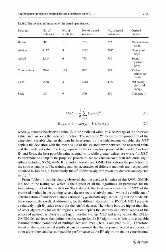
Table 2 The detailed information of the tested open datasets

Datasets No. ofinstances

No. ofattributes

No. of trainedinstances

No. of testedinstances

Desiredoutputs

Boston 506 13 253 253 Median housevalue

Abalone 4177 8 2080 2097 Number ofrings

Airfoil 1503 6 753 750 Soundpressurelevel

Communities 1994 128 997 997 Violentcrimes percapita

CCPP 9568 4 4784 4784 Net hourlyelectricalenergy

Sock 950 9 500 450 Company10

MSE = 1

n

n∑

i=1

(yi−yi )2 (19)

EV AR = 1 − var(yi − yi )/var(yi ) (20)

where yi denotes the observed value, yi is the predicted value, y is the average of the observedvalue, and var(•) is the variance function. The indicator R2 measures the proportion of thedependent variable change that can be interpreted by the independent variable; the MSEdepicts the deviation with the mean value of the squared error between the observed valueand the predicted value; the EVAR represents the explanatory power of the model. For bothR2 and EVAR, the best possible value is equal to 1, while greater values are worse for MSE.Furthermore, to compare the proposed procedure, we took into account four influential algo-rithms including SVM, ANN, RF (random forest), and GMDH to perform the prediction forthe contrast analysis. The training and test accuracies of different methods are, respectivelyobtained in Tables 3, 4. Particularly, the R2 of diverse algorithms on test datasets are depictedin Fig. 7.

From Table 4, it can be clearly observed that the average R2 value of the RVFL-GMDHis 0.668 in the testing set, which is the highest of all the algorithms. In particular, for theforecasting effect of the models on Stock dataset, the final mean square error MSE of theproposed method in the training set and the test set is relatively small, while the coefficient ofdeterminationR2 and the explained varianceEVAR are both large, indicating that themodel fitsthe economic data well. Additionally, for the different datasets, the RVFL-GMDH presentsa relatively high R2 value except for the Airfoil dataset. The whole bars are higher than thatof other algorithms for all the regions, which depicts the stability and effectiveness of theproposed method, as observed in Fig. 7. For the average MSE and EVAR values, the RVFL-GMDH also achieves the optimal results except for the RF algorithm, which is an ensemblelearning method composed of multiple decision trees (Here is assigned as 20). Therefore,based on the experimental results, it can be assumed that the proposed method is superior toother algorithms and has comparable performance as the RF algorithm on the experimental

123

2706 J. Chen et al.

Table3The

training

accuracies

ofpredictin

gthedatasets

Datasets

SVM

ANN

RF

GMDH

RVFL

-GMDH

RM

ER

ME

RM

ER

ME

RM

E

Boston

0.90

90.00

40.91

40.93

90.00

30.93

90.98

20.00

10.98

20.89

10.00

50.89

10.89

10.00

50.89

1

Abalone

0.56

20.00

60.57

80.56

60.00

60.56

60.92

60.00

10.92

60.53

30.00

60.53

30.57

80.00

60.56

2

Airfoil

0.84

10.00

50.84

20.84

80.00

50.84

80.99

30.00

00.99

30.84

20.00

50.84

20.84

20.00

50.84

2

Com

m0.80

30.01

10.80

70.76

80.01

30.76

80.93

70.00

40.93

70.66

50.01

90.66

50.66

70.01

90.66

7

CCPP

Seg

0.93

70.00

30.93

70.93

80.00

30.93

80.99

30.00

10.99

30.93

80.00

30.93

80.93

90.00

30.93

9

Stock

0.95

00.00

30.95

00.98

60.00

00.98

60.99

60.00

00.99

60.94

20.00

30.94

20.99

00.00

10.99

0

Average

0.83

40.00

50.83

80.84

10.00

50.84

10.97

10.00

10.97

10.80

20.00

70.80

20.81

80.00

70.81

5

(R:R

2,M

:MSE

,E:E

VAR)

123

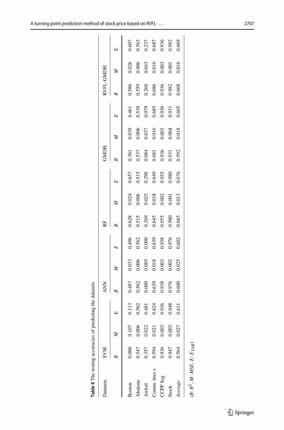
A turning point prediction method of stock price based on RVFL-… 2707

Table4The

testingaccuracies

ofpredictin

gthedatasets

Datasets

SVM

ANN

RF

GMDH

RVFL

-GMDH

RM

ER

ME

RM

ER

ME

RM

E

Boston

0.00

00.10

70.11

30.48

70.03

30.49

60.62

80.02

40.65

70.38

10.03

90.46

10.58

60.02

60.60

7

Abalone

0.54

70.00

60.56

20.56

20.00

60.56

20.51

50.00

60.51

50.53

70.00

60.53

80.55

90.00

60.56

3

Airfoil

0.35

70.02

20.48

10.00

00.08

50.00

00.26

90.02

50.29

80.08

40.03

70.07

90.26

00.04

30.23

7

Com

m.itie

ss

0.59

40.02

10.62

40.63

90.01

80.63

90.64

50.01

80.64

90.68

10.01

60.68

50.68

60.01

60.68

7

CCPP

Seg

0.93

60.00

30.93

60.93

80.00

30.93

80.95

50.00

20.95

50.93

60.00

30.93

60.93

60.00

30.93

6

Stock

0.94

70.00

30.94

80.97

60.00

20.97

60.98

00.00

10.98

00.93

10.00

40.93

10.98

20.00

10.98

2

Average

0.56

40.02

70.61

10.60

00.02

50.60

20.66

50.01

30.67

60.59

20.01

80.60

50.66

80.01

60.66

9

(R:R

2,M

:MSE

,E:E

VAR)

123

2708 J. Chen et al.

Fig. 7 The MSE iteration curve of the proposed approach on Stock dataset

datasets. The proposed procedure basically outperforms the other well-known predictionalgorithms on the experimental dataset, even though the ensemble learning algorithm isadopted.

4.2 Empirical analysis experiment

By obtaining the historical data of stock trading from Yahoo Finance [48], we can randomlychoose the stock price as the analysis object. Here, the Pci-Suntek (stock code: 600,728)and one FTSE-100 index constituent stock, Tesco (stock code: TSCO.L) are selected in ourempirical analysis. The close price of the Pci-Suntek stock from January 2017 to September2018 is obtained and the data normalization is processed as the following Eq. (21).

x(i) = (y(i) − 1

N

N∑

i=1

y(i))

/⎧

⎨

⎩

1

N

N∑

j=1

(y( j) − 1

N

N∑

i=1

y(i))2

⎫

⎬

⎭

1/2

(21)

The chaos of time series is first judged using the method of chaotic attractor determinationreported in Sect. 2. Based on the normalized time series data, them-dimensional phase spacewith the time delay of τ can be constructed, and the point in the phase space is y(t) = x(t),x(t+ τ ),…,x(t + (m−1)τ ). Considering that there are five trading days a week in the stockmarket, we can set the τ value as τ = 5, and the embedding dimension m is taken a positiveinteger such as m = 3, 4,.., 10, etc. Furthermore, for the recent data that has a greater impacton the prediction, the recent data from January 1, 2018 to July 1, 2018 is selected as theverification data and the correlation integral function C(r) is computed in Eq. (3).

The value of the correlation integral is related to the given distance r. Theoretically, thereis a range of r value for the attractor dimension d and the integral function C(r) satisfiesthe log-linear relationship. That is, the d(m0) is equal to the lnCm0(r)/ lnr (see Eq. (5)).Under different embedding dimensions, a series of correlation integral values Cm(r) can becalculated for a series of r values. Taking ln(r) as the horizontal axis and ln(Cm0(r)) as thevertical axis, the graph can be drawn as Fig. 8.

123

A turning point prediction method of stock price based on RVFL-… 2709

Fig. 8 The LnC(r)-ln(r) diagram for Pci-Suntek

As seen in Fig. 8, the curve from top to bottom indicates that the embedding dimensionm= 3, 4, 5,…,10 increases gradually. With the increase of m, the curve becomes steeper andthe slope values are more stable. The obtained stable value is just the estimated value of thecorrelation dimension, and the details are listed in the following Table 5.

It can be visualized from Table 5 that when the embedding dimension m is increased to8, the correlation dimension d(m) tends to be stable. The value is around 3.0, and the bestembedding dimension is 7. This implies that the time series is not a random time series andhas chaotic dynamics characteristics. The correlation value of the chaotic attractor is about3.0. Moreover, the embedding dimension 7 is greater than the 2*3.0287, which satisfies thecondition of restoring the differential homeomorphic dynamical system in Takens’ theorem[31]. Therefore, we can reconstruct the phase space based on the embedded dimension 7.

We take the historical data of Pci-Suntek stock from January 1, 2018 to September 1, 2018,anddivide it into two sections on July1, 2018.The former section is used as the training samplewhile the latter is as the prediction sample. Based on the method mentioned in Sect. 3, we cancompute the turning indicator value, and which is loaded into the RVFL-GMDH network forthe model training. Subsequently, the data from July 1, 2018 to September 1, 2018 is usedas the test data and the turning points of stock prices in this period are predicted. Table 6displays the partial sample data. In particular, it should be noted that the commonly usedapproaches such as ANN and time series methods are chosen to predict the turning points forcomparative analysis. The results of turning point predictions are depicted in Fig. 9. Amongthe figures, Fig. 9a is the trend of the actual stock price, Fig. 9b displays the prediction resultsof the time series method of Auto-Regressive and Moving Average Model (ARMA), Fig. 9cpresents the prediction results of ANN method, and Fig. 9d depicts the prediction results ofthe proposed RVFL-GMDH method.

It can be observed from Fig. 9 that the RVFL-GMDH based turning point predictionmethod has predicted most of the turning points for the samples generally, and the positionof the turning point is basically consistent with the actual trend of the stock price curve.

123

2710 J. Chen et al.

Table5The

estim

ates

ofcorrelationdimension

m1

23

45

67

89

10

d(m

)0.93

421.69

622.60

152.53

502.97

642.70

953.02

873.54

552.74

842.92

81

123

A turning point prediction method of stock price based on RVFL-… 2711

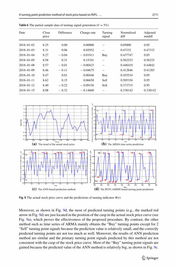
Table 6 The partial sample data of turning signal generation (θ = 5%)

Date Closeprice

Difference Change rate Turningsignal

Normalizeddiff

Adjustednmdiff

2018–01-02 8.25 0.00 0.00000 − 0.05000 0.05

2018–01-03 8.31 0.06 0.02952 − 0.47332 0.47332

2018–01-04 8.27 − 0.04 − 0.01911 Buy 0.437747 0.05

2018–01-05 8.58 0.31 0.15101 − 0.562253 0.56225

2018–01-08 8.57 − 0.01 − 0.00423 − 0.448419 0.44842

2018–01-09 8.46 − 0.11 − 0.04675 − 0.412846 0.41285

2018–01-10 8.47 0.01 0.00446 Buy 0.455534 0.05

2018–01-11 8.62 0.15 0.06658 Sell 0.505336 0.95

2018–01-12 8.40 − 0.22 − 0.09156 Sell 0.373715 0.95

2018–01-15 8.08 − 0.32 − 0.14660 − 0.338142 0.338142

(a) The trend of the actual stock price (b) The ARMA time series prediction

ANN-based prediction method(c) The (d) The RVFL-GMDH based turning point prediction

120 125 130 135 140 145 150 155 160 1656.7

6.8

6.9

7

7.1

7.2

7.3

7.4

7.5

7.6

7.7

Time

Stoc

k Pr

ice

120 125 130 135 140 145 150 155 160 1650

0.1

0.2

0.3

0.4

0.5

0.6

0.7

0.8

0.9

Time

)A

MR

A(d

oht

em

seir

es

emit

rof

rot

aci

dni

gni

nrut

fo

noit

cid

erP

φ(t)

Buy

Sell

120 125 130 135 140 145 150 155 1600.2

0.3

0.4

0.5

0.6

0.7

0.8

0.9

1

Time

dohtem

NN

Ar of

rot ac id nig nin rut

f ono itc ider

Pφ(

t)

Buy

Sell

120 125 130 135 140 145 150 155 160 1650

0.2

0.4

0.6

0.8

1

Time

rot

aci

dni

gni

nrut

fo

eul

av

noit

cid

e rP

φ(t

)

Sell

Buy

Fig. 9 The actual stock price curve and the predictions of turning indicator �(t)

Moreover, as shown in Fig. 9d, the most of predicted turning points (e.g., the marked redarrow in Fig. 9d) are just located in the position of the cusp in the actual stock price curve (seeFig. 9a), which proves the effectiveness of the proposed procedure. By contrast, the othermethod such as time series of ARMA mainly obtains the “Buy” turning points except for 2“Sell” turning point signals because the prediction value is relatively small, and the correctlypredicted turning points are not too much as well. Moreover, the results of ANN predictionmethod are similar and the primary turning point signals predicted by this method are notconsistent with the cusp of the stock price curve. Most of the “Buy” turning point signals aregained because the predicted value of the ANNmethod is relatively big, as shown in Fig. 9c.

123

2712 J. Chen et al.

Table 7 The partial sample data of TSCO.L

Date Closeprice

Difference Changerate

Turningsignal

Normalizeddiff

Adjustednmdiff

2019–01-02 191.55 1.45 0.30 Buy 0.601983 0.05

2019–01-03 199.35 7.8 1.25 Sell 0.763881 0.95

2019–01-04 197.4 − 1.95 − 0.14 Buy 0.515297 0.05

2019–01-07 202.5 5.1 0.42 Buy 0.695043 0.05

2019–01-08 208.1 5.6 0.33 Buy 0.707791 0.05

2019–01-09 211.8 3.7 0.16 Buy 0.659348 0.05

2019–01-10 216.4 4.6 0.17 − 0.682295 0.682295

2019–01-11 218 1.6 0.05 − 0.605808 0.605808

2019–01-14 218 0 0.00 − 0.565014 0.565014

2019–01-15 218.1 0.1 0.00 − 0.567564 0.567564

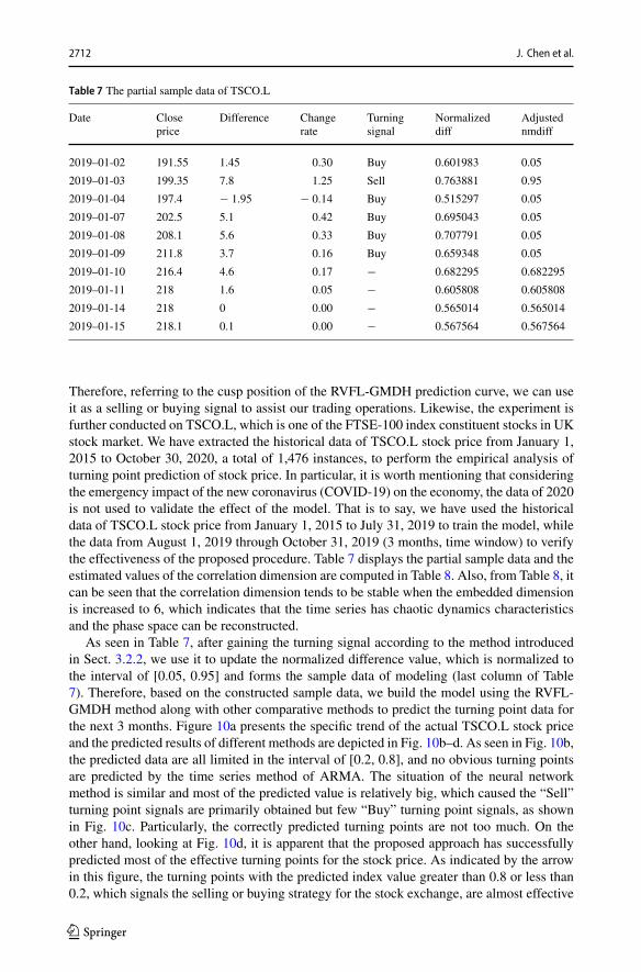
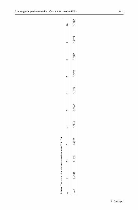
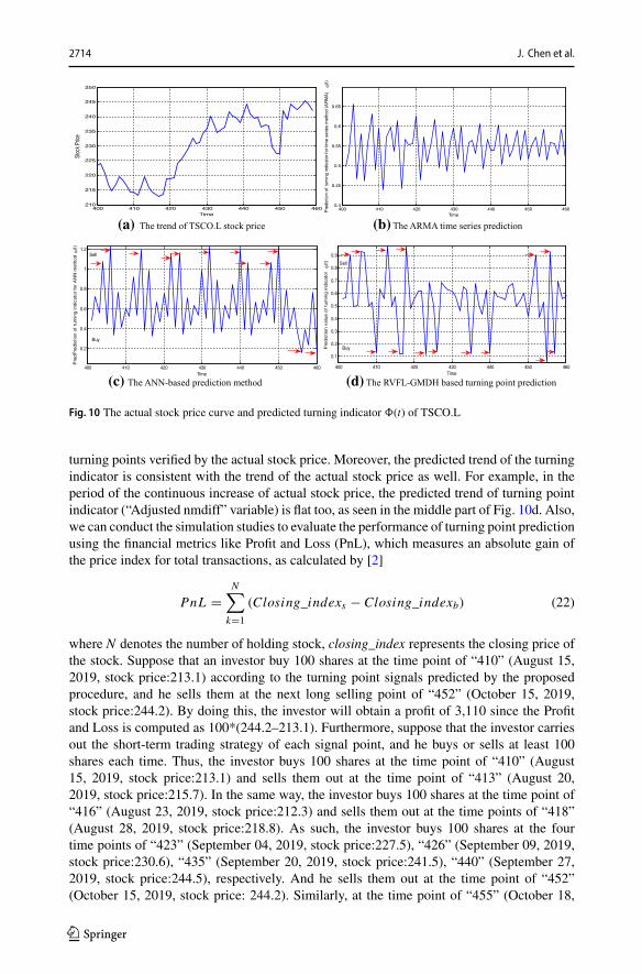
Therefore, referring to the cusp position of the RVFL-GMDH prediction curve, we can useit as a selling or buying signal to assist our trading operations. Likewise, the experiment isfurther conducted on TSCO.L, which is one of the FTSE-100 index constituent stocks in UKstock market. We have extracted the historical data of TSCO.L stock price from January 1,2015 to October 30, 2020, a total of 1,476 instances, to perform the empirical analysis ofturning point prediction of stock price. In particular, it is worth mentioning that consideringthe emergency impact of the new coronavirus (COVID-19) on the economy, the data of 2020is not used to validate the effect of the model. That is to say, we have used the historicaldata of TSCO.L stock price from January 1, 2015 to July 31, 2019 to train the model, whilethe data from August 1, 2019 through October 31, 2019 (3 months, time window) to verifythe effectiveness of the proposed procedure. Table 7 displays the partial sample data and theestimated values of the correlation dimension are computed in Table 8. Also, from Table 8, itcan be seen that the correlation dimension tends to be stable when the embedded dimensionis increased to 6, which indicates that the time series has chaotic dynamics characteristicsand the phase space can be reconstructed.

As seen in Table 7, after gaining the turning signal according to the method introducedin Sect. 3.2.2, we use it to update the normalized difference value, which is normalized tothe interval of [0.05, 0.95] and forms the sample data of modeling (last column of Table7). Therefore, based on the constructed sample data, we build the model using the RVFL-GMDH method along with other comparative methods to predict the turning point data forthe next 3 months. Figure 10a presents the specific trend of the actual TSCO.L stock priceand the predicted results of different methods are depicted in Fig. 10b–d. As seen in Fig. 10b,the predicted data are all limited in the interval of [0.2, 0.8], and no obvious turning pointsare predicted by the time series method of ARMA. The situation of the neural networkmethod is similar and most of the predicted value is relatively big, which caused the “Sell”turning point signals are primarily obtained but few “Buy” turning point signals, as shownin Fig. 10c. Particularly, the correctly predicted turning points are not too much. On theother hand, looking at Fig. 10d, it is apparent that the proposed approach has successfullypredicted most of the effective turning points for the stock price. As indicated by the arrowin this figure, the turning points with the predicted index value greater than 0.8 or less than0.2, which signals the selling or buying strategy for the stock exchange, are almost effective

123

A turning point prediction method of stock price based on RVFL-… 2713

Table8The

correlationdimension

estim

ationof

TSC

O.L

m1

23

45

67

89

10

d(m

)0.97

071.82

262.72

273.66

454.27

673.81

253.52

973.67

073.77

703.81

82

123

2714 J. Chen et al.

(a) The trend of TSCO.L stock price (b) The ARMA time series prediction

(c) The ANN-based prediction method (d) The RVFL-GMDH based turning point prediction

400 410 420 430 440 450 460210

215

220

225

230

235

240

245

250

Time

Stoc

k Pric

e

400 410 420 430 440 450 4600.4

0.45

0.5

0.55

0.6

0.65

Time

)A

MR

A(doh te

mse ires

emit

rofr otacidni

g ninrutfo

noi tciderP

φ(t)

400 410 420 430 440 450 460

0.2

0.4

0.6

0.8

1

1.2

Time

do

hte

mN

NA

rof

rot

ac i

dni

gni

nrut

fo

noit

cid

e rP

der

Pφ(

t)

Buy

Sell

400 410 420 430 440 450 460

0.1

0.2

0.3

0.4

0.5

0.6

0.7

0.8

0.9

Time

Pre

dic

tion v

alu

e o

f tu

rnin

g indic

ato

r φ

(t) Sell

Buy

Fig. 10 The actual stock price curve and predicted turning indicator �(t) of TSCO.L

turning points verified by the actual stock price. Moreover, the predicted trend of the turningindicator is consistent with the trend of the actual stock price as well. For example, in theperiod of the continuous increase of actual stock price, the predicted trend of turning pointindicator (“Adjusted nmdiff” variable) is flat too, as seen in the middle part of Fig. 10d. Also,we can conduct the simulation studies to evaluate the performance of turning point predictionusing the financial metrics like Profit and Loss (PnL), which measures an absolute gain ofthe price index for total transactions, as calculated by [2]

PnL =N

∑

k=1

(Closing_indexs − Closing_indexb) (22)

where N denotes the number of holding stock, closing_index represents the closing price ofthe stock. Suppose that an investor buy 100 shares at the time point of “410” (August 15,2019, stock price:213.1) according to the turning point signals predicted by the proposedprocedure, and he sells them at the next long selling point of “452” (October 15, 2019,stock price:244.2). By doing this, the investor will obtain a profit of 3,110 since the Profitand Loss is computed as 100*(244.2–213.1). Furthermore, suppose that the investor carriesout the short-term trading strategy of each signal point, and he buys or sells at least 100shares each time. Thus, the investor buys 100 shares at the time point of “410” (August15, 2019, stock price:213.1) and sells them out at the time point of “413” (August 20,2019, stock price:215.7). In the same way, the investor buys 100 shares at the time point of“416” (August 23, 2019, stock price:212.3) and sells them out at the time points of “418”(August 28, 2019, stock price:218.8). As such, the investor buys 100 shares at the fourtime points of “423” (September 04, 2019, stock price:227.5), “426” (September 09, 2019,stock price:230.6), “435” (September 20, 2019, stock price:241.5), “440” (September 27,2019, stock price:244.5), respectively. And he sells them out at the time point of “452”(October 15, 2019, stock price: 244.2). Similarly, at the time point of “455” (October 18,

123

A turning point prediction method of stock price based on RVFL-… 2715

2019, stock price: 244), the investor buys 100 shares and sells them out at the time point of“456” (October 21, 2019, stock price: 245.5). In this manner, the PnL of the trading strategybased on turning point signals in this time window can be calculated as 100*(215.7–213.1)+ 100*(218.8–212.3) + 100*(4*244.2–227.5–230.6–241.5–244.5) + 100*(245.5–244) =4,330. In summary, the results of the empirical analysis reveal the feasibility and effectivenessof the proposed procedure, which is successful in predicting the turning points of stock timeseries and can also be employed in more real-world application scenarios.

5 Conclusions

This work proposes a novel turning point prediction approach for the time series analysisof stock price. The modeling of the nonlinear dynamic system based on the RVFL-GMDHnetwork is introduced in the paper, and the chaos theory is utilized to analyze the time series.Using the fractal characteristic of strange attractor with infinite self-similar structure, thetrajectory trend prediction in the reconstructed phase space is accomplished. This methodnot only exploits the prediction ability brought by the periodic denseness in chaotic dynamicsystems but also avoids the issue that the single predicted value is not accurate due to the sen-sitivity of the initial value. A series of experiments are performed for the proposed approachon both the open dataset and practical stock price data. The experimental findings demon-strate the effectiveness of the model compared to the other state-of-art methods and presentthe proposed procedure with the substantial performance for forecasting the turning pointsof stock time series in real-life application scenarios. Based on the experimental analysis,it can be concluded that the proposed procedure has a significant capability for the turningpoint prediction of stock price and can also be extended to other fields such as electricity loadforecasting, material demand planning, and international oil price forecast. In future devel-opment, we plan to deploy it on embedded systems to form the production for automaticallypredicting and recognizing the turning points of stock prices. Meanwhile, we intend to applyit to more real-world applications.

Supplementary Information The online version contains supplementary material available at https://doi.org/10.1007/s10115-021-01602-3.

Acknowledgements The authors express their acknowledges to the Data Mining and Computing IntelligenceResearch Group at Xiamen University for funding this work through grant No. of 20720181004 and 61672439separately. The authors also thank the expert, Mr. Zhang Liang-jun from Tiptech Ltd., for the beneficialdiscussion and assistance. The authors are thankful to the editors and all the anonymous reviewers for theircritically reviewing and constructive suggestions.

References

1. ShenW, GuoX,WuC,WuD (2011) Forecasting stock indices using radial basis function neural networksoptimized by artificial fish swarm algorithm. Knowl-Based Syst 24(3):378–385

2. Chen TL, Chen FY (2016) An intelligent pattern recognition model for supporting investment decisionsin stock market. Inf Sci 346:261–274

3. Babu CN, Reddy BE (2015) Prediction of selected Indian stock using a partitioning–interpolation basedARIMA–GARCH model. Appl Comput Informat 11(2):130–143

4. Hamzaçebi C, Pekkaya M (2011) Determining of stock investments with grey relational analysis. ExpertSyst Appl 38(8):9186–9195

5. Wen D, Wang GJ, Ma C, Wang Y (2019) Risk spillovers between oil and stock markets: a VAR for VaRanalysis. Energy Econom 80:524–535

123

2716 J. Chen et al.

6. LongW,LuZ,Cui L (2019)Deep learning-based feature engineering for stock pricemovement prediction.Knowl-Based Syst 164:163–173

7. Dash R, Dash PK (2016) A hybrid stock trading framework integrating technical analysis with machinelearning techniques. The Journal of Finance and Data Science 2(1):42–57

8. Fujimaki R, Nakata T, Tsukahara H, Sato A, Yamanishi K (2009) Mining abnormal patterns from het-erogeneous time-series with irrelevant features for fault event detection. Statist Analy Data Mining: TheASA Data Sci J 2(1):1–17

9. Nahil A, Lyhyaoui A (2018) Short-term stock price forecasting using kernel principal component analysisand support vector machines: the case of Casablanca stock exchange. Procedia Comput Sci 127:161–169

10. Lahmiri S (2018) Minute-ahead stock price forecasting based on singular spectrum analysis and supportvector regression. Appl Math Comput 320:444–451

11. Chang, P. C., Fan, C. Y., & Liu, C. H. (2008). Integrating a piecewise linear representation method anda neural network model for stock trading points prediction. IEEE Trans Syst, Man, Cybernet, Part C(Applications and Reviews), 39(1), 80–92

12. Göçken M, Özçalıcı M, Boru A, Dosdogru AT (2016) Integrating metaheuristics and artificial neuralnetworks for improved stock price prediction. Expert Syst Appl 44:320–331

13. Efendi R, Arbaiy N, Deris MM (2018) A new procedure in stock market forecasting based on fuzzyrandom auto-regression time series model. Inf Sci 441:113–132

14. Cheng SH, Chen SM, Jian WS (2016) Fuzzy time series forecasting based on fuzzy logical relationshipsand similarity measures. Inf Sci 327:272–287

15. Kim Y, Jeong SR, Ghani I (2014) Text opinion mining to analyze news for stock market prediction. Int JAdv Soft Comput Appl 6(1):2074–8523

16. Nikfarjam, A., Emadzadeh, E., & Muthaiyah, S. (2010, February). Text mining approaches for stockmarket prediction. In 2010 The 2nd international conference on computer and automation engineering(ICCAE) (Vol. 4, pp. 256–260). IEEE

17. White, H. (1988, July). Economic prediction using neural networks: The case of IBM daily stock returns.In ICNN (Vol. 2, pp. 451–458)

18. Baba, N., & Kozaki, M. (1992, June). An intelligent forecasting system of stock price using neuralnetworks. In [Proceedings 1992] IJCNN International Joint Conference on Neural Networks (Vol. 1,pp. 371–377). IEEE

19. de Oliveira FA, Nobre CN, Zárate LE (2013) Applying Artificial Neural Networks to prediction of stockprice and improvement of the directional prediction index–Case study of PETR4, Petrobras. Brazil Expertsyst appl 40(18):7596–7606

20. Laboissiere LA, Fernandes RA, Lage GG (2015) Maximum and minimum stock price forecasting ofBrazilian power distribution companies based on artificial neural networks. Appl Soft Comput 35:66–74

21. Sayavong, L., Wu, Z., & Chalita, S. (2019, September). Research on stock price prediction method basedon convolutional neural network. In 2019 International Conference on Virtual Reality and IntelligentSystems (ICVRIS) (pp. 173–176). IEEE

22. Tsantekidis, A., Passalis, N., Tefas, A., Kanniainen, J., Gabbouj, M., & Iosifidis, A. (2017, July). Fore-casting stock prices from the limit order book using convolutional neural networks. In 2017 IEEE 19thConference on Business Informatics (CBI) (Vol. 1, pp. 7–12). IEEE

23. Deng Y, Bao F, Kong Y, Ren Z, Dai Q (2016) Deep direct reinforcement learning for financial signalrepresentation and trading. IEEE Trans Neural Netw Learn Syst 28(3):653–664

24. Zarkias, K. S., Passalis, N., Tsantekidis, A., & Tefas, A. (2019, May). Deep reinforcement learning forfinancial trading using price trailing. In ICASSP 2019–2019 IEEE International Conference on Acoustics,Speech and Signal Processing (ICASSP) (pp. 3067–3071). IEEE

25. Rather AM, Agarwal A, Sastry VN (2015) Recurrent neural network and a hybrid model for predictionof stock returns. Expert Syst Appl 42(6):3234–3241

26. DixonM (2018) Sequence classification of the limit order book using recurrent neural networks. J ComputSci 24:277–286

27. TangH, Dong P, Shi Y (2019) A new approach of integrating piecewise linear representation andweightedsupport vector machine for forecasting stock turning points. Appl Soft Comput 78:685–696

28. Intachai, P.,&Yuvapoositanon, P. (2017,March). The variable forgetting factor-based local averagemodelalgorithm for prediction of financial time series. In 2017 International Electrical Engineering Congress(iEECON) (pp. 1–4). IEEE

29. Chang PC, Liao TW, Lin JJ, Fan CY (2011) A dynamic threshold decision system for stock trading signaldetection. Appl Soft Comput 11(5):3998–4010

30. Takens, F. (1981). Detecting strange attractors in turbulence. In Dynamical systems and turbulence,Warwick 1980 (pp. 366–381). Springer, Berlin, Heidelberg.

123

A turning point prediction method of stock price based on RVFL-… 2717

31. KolmogorovAN (1963) On the representation of continuous functions ofmany variables by superpositionof continuous functions of one variable and addition. Trans Am Math Soc 2(28):55–59

32. Pao YH, Park GH, Sobajic DJ (1994) Learning and generalization characteristics of the random vectorfunctional-link net. Neurocomputing 6(2):163–180

33. Ren Y, Suganthan PN, Srikanth N, Amaratunga G (2016) Random vector functional link network forshort-term electricity load demand forecasting. Inf Sci 367:1078–1093

34. Gorban AN, Tyukin IY, Prokhorov DV, Sofeikov KI (2016) Approximation with random bases: pro etcontra. Inf Sci 364:129–145

35. Scardapane S, Wang D, Uncini A (2017) Bayesian random vector functional-link networks for robustdata modeling. IEEE Trans Cybernet 48(7):2049–2059

36. Cui W, Zhang L, Li B, Guo J, Meng W, Wang H, Xie L (2017) Received signal strength based indoorpositioning using a random vector functional link network. IEEE Trans Industr Inf 14(5):1846–1855

37. Zhang PB, Yang ZX (2020) A new learning paradigm for random vector functional-link network: RVFL+.Neural Netw 122:94–105

38. HuangGB,ZhuQY,SiewCK(2006)Extreme learningmachine: theory and applications.Neurocomputing70(1–3):489–501

39. Rahimi, A., & Recht, B. (2008, December). Weighted sums of random kitchen sinks: replacing mini-mization with randomization in learning. In Nips (pp. 1313–1320)

40. Mueller, J. A., & Lemke, F. (2000). Self-organising data mining: an intelligent approach to extract knowl-edge from data. Hamburg: Libri.

41. He CZ, Wu J, Müller JA (2008) Optimal cooperation between external criterion and data division inGMDH. Int J Syst Sci 39(6):601–606

42. TengGE, He CZ, Xiao J, Jiang XY (2013) Customer credit scoring based onHMM/GMDHhybridmodel.Knowl Inf Syst 36(3):731–747

43. Anaconda. Available online: https://www.anaconda.com/ (accessed on 17 Nov., 2019)44. scikit-learn. Available online: https://scikit-learn.org/stable/ (accessed on 17 Nov., 2019)45. PyMC3. Available online: https://docs.pymc.io/ (accessed on 17 Nov., 2019)46. Blake, C. (1998). UCI repository of machine learning databases. http://www.ics.uci.edu/~mlearn/

MLRepository.html47. Alcalá-Fdez, J., Fernández, A., Luengo, J., Derrac, J., García, S., Sánchez, L., & Herrera, F. (2011).

Keel data-mining software tool: data set repository, integration of algorithms and experimental analysisframework. Journal of Multiple-Valued Logic & Soft Computing, 17

48. https://fiance.yahoo.com/quote/600728.SS/history?p=600728.SS

Publisher’s Note Springer Nature remains neutral with regard to jurisdictional claims in published maps andinstitutional affiliations.

Junde Chen receives his bachelor degree from Xiangtan University, and the master degree from Sichuan Uni versity separately . Hisresearch interests include the aspects of Data Mining, Image Process-ing, Machine Learning and Decision Support System etc. Currently, hei s doing PHD in School of Informatics , Xiamen University , Xiamencity, in China Shuangyuan

123

2718 J. Chen et al.

Shuangyuan Yang received the PHD degree in School of computerscience, Huazhong University of science and technology, and she iscurrently working at the School of Informat ics, Xiamen University.His research interests include Machine Learning, Computer Vision,Information Extraction & Retrieval, Natural Language Processing, andData Mining Technology etc.

Defu Zhang works in School of Informatics at Xiamen University cur-rently. His research interests include all aspects of computational intel-ligence, image analysis and data mining, etc. He has published papersin the following Journals: INFORMS Journal on Computing, Comput-ers Operations Research, European Journal of Operational Research,Expert System with Applications, etc.

Y. A. Nanehkaran received the B.E. degree from IAU of ArdabilBranch, Ardabil, Iran, in Power Electrical Engineering and M.Sc.degree in IT from Cankaya University, Ankara, Turkey. He is currentlypursuing the Ph.D. degree in the Department of Computer Science atXiamen University, Xiamen city, in China. His research area mainlyincludes data mining, big data and deep learning techniques.

123