A tree traversal algorithm for decision problems

in knot theory and 3-manifold topology∗

Benjamin A. Burton and Melih Ozlen

Author’s self-archived version

Available from http://www.maths.uq.edu.au/~bab/papers/

Abstract

In low-dimensional topology, many important decision algorithms are based on nor-mal surface enumeration, which is a form of vertex enumeration over a high-dimensionaland highly degenerate polytope. Because this enumeration is subject to extra combi-natorial constraints, the only practical algorithms to date have been variants of theclassical double description method. In this paper we present the first practical nor-mal surface enumeration algorithm that breaks out of the double description paradigm.This new algorithm is based on a tree traversal with feasibility and domination tests,and it enjoys a number of advantages over the double description method: incremen-tal output, significantly lower time and space complexity, and a natural suitability forparallelisation.

ACM classes F.2.2; G.1.6; G.4

Keywords Normal surfaces, vertex enumeration, tree traversal, backtracking, linearprogramming

1 Introduction

Much research in low-dimensional topology is driven by decision problems. Examples fromknot theory include the unknot recognition and knot equivalence problems, and analogousexamples from 3-manifold topology include 3-sphere recognition and the homeomorphismproblem.

Significant progress has been made on these problems over the past 50 years. For in-stance, Haken introduced an algorithm for recognising the unknot in the 1960s [17], andRubinstein presented the first 3-sphere recognition algorithm in the 1990s [26]. Since Perel-man’s proof of the geometrisation conjecture [22], we now have a complete (but extremelycomplex) algorithm for the homeomorphism problem, pieced together though a diverse arrayof techniques [20, 24].

A key problem remains with many 3-dimensional decision algorithms (including all ofthose mentioned above): the best known algorithms run in exponential time (and for someproblems, worse), where the input size is measured by the number of crossings in a knotdiagram, or the number of tetrahedra in a 3-manifold triangulation. This severely limitsthe practicality of such algorithms. For example, it took 30 years to resolve Thurston’swell-known conjecture regarding the Weber-Seifert space [5]—an algorithmic solution was

∗This is the shorter conference version, as presented at the 27th Annual Symposium on ComputationalGeometry. See arXiv:1010.6200 for the full version of this paper.

1

found in 1984, but it took 25 more years of development before the algorithm became usable[12, 21]. The input size was n = 23.

The most successful machinery for 3-dimensional decision problems has been normalsurface theory. Normal surfaces were introduced by Kneser [23] and later developed byHaken for algorithmic use [17, 18], and they play a key role in all of the decision algorithmsmentioned above. In essence, they allow us to convert difficult “topological searches” intoa “combinatorial search” in which we enumerate vertices of a high-dimensional polytopecalled the projective solution space.1 In Section 2 we outline the essential properties of theprojective solution space; see [19] for a broader introduction to normal surface theory in atopological setting.

For many topological decision problems, the computational bottleneck is precisely thisvertex enumeration. Vertex enumeration over a polytope is a well-studied problem, andseveral families of algorithms appear in the literature. These include backtracking algorithms[4, 16], pivot-based reverse search algorithms [1, 3, 15], and the inductive double descriptionmethod [25]. All have worst-case running times that are super-polynomial in both theinput and the output size, and it is not yet known whether a polynomial time algorithm(with respect to the combined input and output size) exists.2 For topological problems, thecorresponding running times are exponential in the “topological input size”; that is, thenumber of crossings or tetrahedra.

Normal surface theory poses particular challenges for vertex enumeration. The projectivesolution space is a highly degenerate (or non-simple) polytope, and exact rational arithmeticis required for topological reasons. Moreover, we are not interested in all of the vertices ofthe projective solution space, but just those that satisfy a powerful set of conditions calledthe quadrilateral constraints. These are extra combinatorial constraints that eliminate allbut a small fraction of the polytope, and an effective enumeration algorithm should be ableto enforce them as it goes, not simply use them as a post-processing output filter.

All well-known implementations of normal surface enumeration [6, 14] are based on thedouble description method: degeneracy and exact arithmetic do not pose any difficulties,and it is simple to embed the quadrilateral constraints directly into the algorithm [10].Section 2 includes a discussion of why backtracking and reverse search algorithms have notbeen used to date. Nevertheless, the double description method does suffer from significantdrawbacks:

• It can suffer from a combinatorial explosion: even if both the input and output sizesare small, it can build extremely complex intermediate polytopes where the numberof vertices is super-polynomial in both the input and output sizes. This leads to anunwelcome explosion in both time and memory usage, which is frustrating for normalsurface enumeration where the output size is often small (though still exponential ingeneral) [8].

• The double description method is difficult to parallelise, due to its inductive nature.There have been recent efforts [27], though they rely on a shared memory model, andfor some polytopes the speed-up factor plateaus when the number of processors growslarge.

• Because of its inductive nature, the double description method typically does notoutput any vertices until the entire algorithm is complete. This effectively removesthe possibility of early termination, which is desirable for many topological algorithms.

1For some problems, instead of enumerating vertices we must enumerate a Hilbert basis for a polyhedralcone.

2Efficient algorithms do exist for certain classes of polytopes, in particular for non-degenerate polytopes[3].

2

In this paper we present a new algorithm for normal surface enumeration. This algorithmbelongs to the backtracking family, and is described in detail in Section 3. Globally, thealgorithm is structured as a tree traversal, where the underlying tree is a decision treeindicating which coordinates are zero and which are non-zero. Locally, we move throughthe tree by performing incremental feasibility tests using the dual simplex method (thoughinterior point methods could equally well be used).

Fukuda et al. [16] discuss an impediment to backtracking algorithms, which is the needto solve the NP-complete restricted vertex problem. We circumvent this by ordering the treetraversal in a careful way and introducing domination tests over the set of previously-foundvertices. This introduces super-polynomial time and space costs, but for normal surfaceenumeration this trade-off is typically not severe (we quantify this within Sections 4 and 5).

Our algorithm is well-suited to normal surface enumeration, since it integrates the quadri-lateral constraints seamlessly into the tree structure. More significantly, it is the first normalsurface enumeration algorithm to break out of the double description paradigm. Further-more, it enjoys a number of advantages over previous algorithms:

• The theoretical worst-case bounds on both time and space complexity are significantlybetter for the new algorithm. In particular, the space complexity is a small polynomialin the combined input and output size. See Section 4 for details.

• The new algorithm lends itself well to parallelisation, including both shared memorymodels and distributed processing, with minimal inter-communication and synchroni-sation.

• The new algorithm produces incremental output, which makes it well-suited for earlytermination and further parallelisation.

• The tree traversal supports a natural sense of “progress tracking”, so that users cangain a rough sense for how far they are through the enumeration procedure.

In Section 5 we measure the performance of the new algorithm against the prior stateof the art, using a rich test suite with hundreds of problems that span a wide range ofdifficulties. For simple problems we find the new algorithm slower, but as the problemsbecome more difficult the new algorithm quickly outperforms the old, often running ordersof magnitude faster. We conclude that for difficult problems this new tree traversal algorithmis superior, owing to both its stronger practical performance and its desirable theoreticalattributes as outlined above.

2 Preliminaries

For decision problems based on normal surface theory, the input is a 3-manifold triangula-tion.3 This is a collection of n tetrahedra where some or all of the 4n faces are affinely iden-tified (or “glued together”) in pairs, so that the resulting topological space is a 3-manifold.The input size is measured by the number of tetrahedra, which we denote by n throughoutthis paper.

We allow two faces of the same tetrahedron to be identified together; likewise, we allowdifferent edges or vertices of the same tetrahedron to be identified. Some authors refer tosuch triangulations as semi-simplicial triangulations or pseudo-triangulations. In essence,we allow the tetrahedra to be “bent” or “twisted”, instead of insisting that they be rigidlyembedded in some larger space. This more flexible definition allows us to keep the inputsize n small, which is important when dealing with exponential algorithms.

3In knot theory we triangulate the knot complement—that is, the 3-dimensional space surrounding theknot.

3

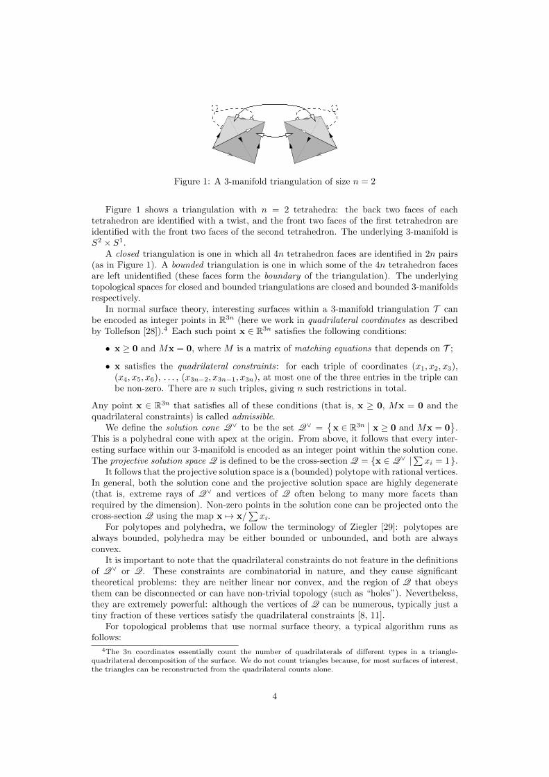
Figure 1: A 3-manifold triangulation of size n = 2

Figure 1 shows a triangulation with n = 2 tetrahedra: the back two faces of eachtetrahedron are identified with a twist, and the front two faces of the first tetrahedron areidentified with the front two faces of the second tetrahedron. The underlying 3-manifold isS2 × S1.

A closed triangulation is one in which all 4n tetrahedron faces are identified in 2n pairs(as in Figure 1). A bounded triangulation is one in which some of the 4n tetrahedron facesare left unidentified (these faces form the boundary of the triangulation). The underlyingtopological spaces for closed and bounded triangulations are closed and bounded 3-manifoldsrespectively.

In normal surface theory, interesting surfaces within a 3-manifold triangulation T canbe encoded as integer points in R3n (here we work in quadrilateral coordinates as describedby Tollefson [28]).4 Each such point x ∈ R3n satisfies the following conditions:

• x ≥ 0 and Mx = 0, where M is a matrix of matching equations that depends on T ;

• x satisfies the quadrilateral constraints: for each triple of coordinates (x1, x2, x3),(x4, x5, x6), . . . , (x3n−2, x3n−1, x3n), at most one of the three entries in the triple canbe non-zero. There are n such triples, giving n such restrictions in total.

Any point x ∈ R3n that satisfies all of these conditions (that is, x ≥ 0, Mx = 0 and thequadrilateral constraints) is called admissible.

We define the solution cone Q∨ to be the set Q∨ ={

x ∈ R3n∣∣ x ≥ 0 and Mx = 0

}.

This is a polyhedral cone with apex at the origin. From above, it follows that every inter-esting surface within our 3-manifold is encoded as an integer point within the solution cone.The projective solution space Q is defined to be the cross-section Q = {x ∈ Q∨ |

∑xi = 1}.

It follows that the projective solution space is a (bounded) polytope with rational vertices.In general, both the solution cone and the projective solution space are highly degenerate(that is, extreme rays of Q∨ and vertices of Q often belong to many more facets thanrequired by the dimension). Non-zero points in the solution cone can be projected onto thecross-section Q using the map x 7→ x/

∑xi.

For polytopes and polyhedra, we follow the terminology of Ziegler [29]: polytopes arealways bounded, polyhedra may be either bounded or unbounded, and both are alwaysconvex.

It is important to note that the quadrilateral constraints do not feature in the definitionsof Q∨ or Q. These constraints are combinatorial in nature, and they cause significanttheoretical problems: they are neither linear nor convex, and the region of Q that obeysthem can be disconnected or can have non-trivial topology (such as “holes”). Nevertheless,they are extremely powerful: although the vertices of Q can be numerous, typically just atiny fraction of these vertices satisfy the quadrilateral constraints [8, 11].

For topological problems that use normal surface theory, a typical algorithm runs asfollows:

4The 3n coordinates essentially count the number of quadrilaterals of different types in a triangle-quadrilateral decomposition of the surface. We do not count triangles because, for most surfaces of interest,the triangles can be reconstructed from the quadrilateral counts alone.

4

1. Enumerate all admissible vertices of the projective solution space Q (that is, all verticesof Q that satisfy the quadrilateral constraints);

2. Scale each vertex to its smallest integer multiple, “decode” it to obtain a surface withinthe underlying 3-manifold triangulation, and test whether this surface is “interesting”;

3. Terminate the algorithm once an interesting surface is found or all vertices are ex-hausted.

The meaning of “interesting” varies for different decision problems. For more of the topo-logical context see [19]; for more on quadrilateral coordinates and the projective solutionspace see [7].

As indicated in the introduction, step 1 (the enumeration of vertices) is typically thecomputational bottleneck. Because so few vertices are admissible, it is crucial for normalsurface enumeration algorithms to enforce the quadrilateral constraints as they go—onecannot afford to enumerate the entire vertex set of Q (which is generally orders of magnitudelarger) and then enforce the quadrilateral constraints afterwards.

Traditionally, normal surface enumeration algorithms are based on the double descriptionmethod of Motzkin et al. [25], with additional algorithmic improvements specific to normalsurface theory [10]. In brief, we construct a sequence of polytopes P0, P1, . . . , Pe, where P0

is the unit simplex in R3n, Pe is the final solution space Q, and each intermediate polytopePi is the intersection of the unit simplex with the first i matching equations. The algorithmworks inductively, constructing Pi+1 from Pi at each stage. For each intermediate polytopePi we throw away any vertices that do not satisfy the quadrilateral constraints, and it canbe shown inductively that this yields the correct final solution set.

Other methods of vertex enumeration include backtracking and reverse search algorithms.It is worth noting why these have not been used for normal surface enumeration to date:

• Reverse search algorithms map out vertices by pivoting along edges of the polytope.This makes it difficult to incorporate the quadrilateral constraints: since the regionthat satisfies these constraints can be disconnected, we may need to pivot throughvertices that break these constraints in order to map out all solutions. Degeneracy canalso cause significant performance problems for reverse search algorithms [1, 2].

• Backtracking algorithms receive comparatively little attention in the literature. Fukudaet al. [16] show that backtracking can solve the face enumeration problem in polyno-mial time. However, for vertex enumeration their framework requires a solution tothe NP-complete restricted vertex problem, and they conclude that straightforwardbacktracking is unlikely to work efficiently for vertex enumeration in general.

Our new algorithm belongs to the backtracking family. Despite the concerns of Fukudaet al., we find that for large problems our algorithm is a significant improvement overthe prior state of the art, often running orders of magnitude faster. We achieve this byintroducing domination tests, a trade-off that increases time and space costs but allowsus to avoid solving the restricted vertex problem directly. The full algorithm is given inSection 3 below.

3 The tree traversal algorithm

The basic idea behind the algorithm is to construct admissible vertices x ∈ Q by iteratingthrough all possible combinations of which coordinates xi are zero and which coordinatesxi are non-zero. We arrange these combinations into a search tree of height n, which wetraverse in a depth-first manner. Using a combination of feasibility tests and domination

5

tests, we are able to prune this search tree so that the traversal is more efficient, and so thatthe leaves at depth n correspond precisely to the admissible vertices of Q.

Because the quadrilateral constraints are expressed purely in terms of zero versus non-zero coordinates, we can easily build the quadrilateral constraints directly into the structureof the search tree. We do this with the help of type vectors, which we introduce in Section 3.1.In Section 3.2 we describe the search tree and present the overall structure of the algorithm.Proofs of all results in this section can be found in the full version of this paper.

3.1 Type vectors

Recall the quadrilateral constraints, which state that for each i = 1, . . . , n, at most one ofthe three coordinates x3i−2, x3i−1, x3i can be non-zero. A type vector is a sequence of nsymbols that indicates how these constraints are resolved for each i. In detail:

Definition (Type vector). Let x = (x1, . . . , x3n) ∈ R3n be any vector that satisfies thequadrilateral constraints. We define the type vector of x as τ(x) = (τ1, . . . , τn) ∈ {0, 1, 2, 3}n,where

τi =

0 if x3i−2 = x3i−1 = x3i = 0;1 if x3i−2 6= 0 and x3i−1 = x3i = 0;2 if x3i−1 6= 0 and x3i−2 = x3i = 0;3 if x3i 6= 0 and x3i−2 = x3i−1 = 0.

(1)

For example, if n = 4 and x = (0, 1, 0, 0, 0, 4, 0, 0, 0, 0, 0, 2) ∈ R12, then τ(x) =(2, 3, 0, 3). An important feature of type vectors is that they carry enough information tocompletely reconstruct any vertex of the projective solution space, as shown by the followingresult.

Lemma 1. Let x be any admissible vertex of Q. Then the precise coordinates x1, . . . , x3n canbe recovered from the type vector τ(x) by simultaneously solving (i) the matching equationsMx = 0; (ii) the projective equation

∑xi = 1; and (iii) the equations of the form xj = 0

as dictated by (1) above, according to the particular value (0, 1, 2 or 3) of each entry in thetype vector τ(x).

Note that this full recovery of x from τ(x) is only possible for vertices of Q, not arbitrarypoints of Q. In general, the type vector τ(x) carries only enough information for us todetermine the smallest face of Q to which x belongs.

However, type vectors do carry enough information for us to identify which admissiblepoints x ∈ Q are vertices of Q. For this we introduce the concept of domination5.

Definition (Domination). Let τ, σ ∈ {0, 1, 2, 3}n be type vectors. We say that τ dominatesσ if, for each i = 1, . . . , n, either σi = τi or σi = 0. We write this as τ ≥ σ.

For example, if n = 4 then (1, 0, 2, 3) ≥ (1, 0, 2, 0) ≥ (1, 0, 2, 0) ≥ (1, 0, 0, 0). On theother hand, neither of (1, 0, 2, 0) or (1, 0, 3, 0) dominates the other. It is clear that in general,domination imposes a partial order (but not a total order) on type vectors.

We can characterise admissible vertices of the projective solution space entirely in termsof type vectors and domination, as seen in the following result.

Lemma 2. Let x ∈ Q be admissible. Then the following statements are equivalent:

• x is a vertex of Q;

• there is no admissible point y ∈ Q for which τ(x) ≥ τ(y) and x 6= y;

5We use the word “domination” because domination of type vectors corresponds precisely to dominationin the face lattice of the polytope Q. See the full version of this paper for details.

6

• there is no admissible vertex y of Q for which τ(x) ≥ τ(y) and x 6= y.

Because our algorithm involves backtracking, it spends much of its time working withpartially-constructed type vectors. It is therefore useful to formalise this notion.

Definition (Partial type vector). A partial type vector is any vector τ = (τ1, . . . , τn), whereeach τi ∈ {0, 1, 2, 3,−}. We call the special symbol “−” the unknown symbol. A partial typevector that does not contain any unknown symbols is also referred to as a complete typevector.

We say that two partial type vectors τ and σ match if, for each i = 1, . . . , n, eitherτi = σi or at least one of τi, σi is the unknown symbol.

For example, (1,−, 2) and (1, 3, 2) match, and (1,−, 2) and (1, 3,−) also match. However,(1,−, 2) and (0,−, 2) do not match because their leading entries conflict. If τ and σ areboth complete type vectors, then τ matches σ if and only if τ = σ.

Definition (Type constraints). Let τ = (τ1, . . . , τn) ∈ {0, 1, 2, 3,−}n be a partial typevector. The type constraints for τ are a collection of equality constraints and non-strictinequality constraints on an arbitrary point x = (x1, . . . , x3n) ∈ R3n. For each i = 1, . . . , n,the type symbol τi contributes the following constraints to this collection:

x3i−2 = x3i−1 = x3i = 0 if τi = 0;x3i−2 ≥ 1 and x3i−1 = x3i = 0 if τi = 1;x3i−1 ≥ 1 and x3i−2 = x3i = 0 if τi = 2;x3i ≥ 1 and x3i−2 = x3i−1 = 0 if τi = 3;no constraints if τi = −.

Note that, unlike all of the other constraints seen so far, the type constraints are notinvariant under scaling. The type constraints are most useful in the solution cone Q∨, whereany admissible point x ∈ Q∨ with xj > 0 can be rescaled to some admissible point λx ∈ Q∨

with λxj ≥ 1. We see this scaling behaviour in Lemma 3 below.The type constraints are similar but not identical to the conditions described by equa-

tion (1) for the type vector τ(x), and their precise relationship is described by the followinglemma. The key difference is that (1) uses strict inequalities of the form xj > 0, whereasthe type constraints use non-strict inequalities of the form xj ≥ 1. This is because we usethe type constraints with techniques from linear programming, where non-strict inequalitiesare simpler to deal with.

Lemma 3. Let σ ∈ {0, 1, 2, 3,−}n be any partial type vector. If x ∈ R3n satisfies the typeconstraints for σ, then τ(x) matches σ. Conversely, if x ∈ R3n is an admissible vector forwhich τ(x) matches σ, then λx satisfies the type constraints for σ for some scalar λ > 0.

We finish this section on type vectors with a simple but important note.

Lemma 4. There is no x ∈ Q for which τ(x) is the zero vector.

3.2 The structure of the algorithm

Recall that our plan is to iterate through all possible combinations of zero and non-zerocoordinates. We do this by iterating through all possible type vectors, which implicitlyenforces the quadrilateral constraints as we go. The framework for this iteration is the typetree.

Definition (Type tree). The type tree is a rooted tree of height n, where all leaf nodesare at depth n, and where each non-leaf node has precisely four children. The four edgesdescending from each non-leaf node are labelled 0, 1, 2 and 3 respectively.

7

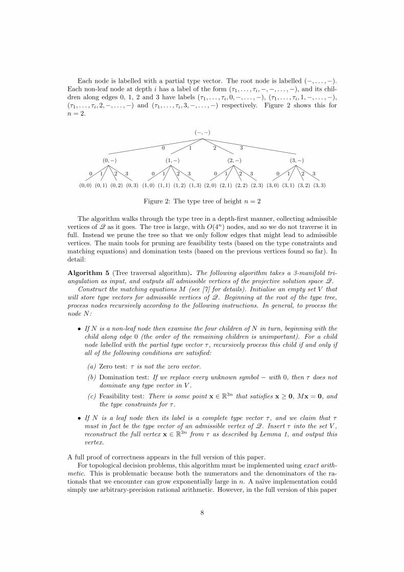
Each node is labelled with a partial type vector. The root node is labelled (−, . . . ,−).Each non-leaf node at depth i has a label of the form (τ1, . . . , τi,−,−, . . . ,−), and its chil-dren along edges 0, 1, 2 and 3 have labels (τ1, . . . , τi, 0,−, . . . ,−), (τ1, . . . , τi, 1,−, . . . ,−),(τ1, . . . , τi, 2,−, . . . ,−) and (τ1, . . . , τi, 3,−, . . . ,−) respectively. Figure 2 shows this forn = 2.

0000

0

1111

1

2222

2

3333

3

(−,−)

(0,−) (1,−) (2,−) (3,−)

(0, 0) (0, 1) (0, 2) (0, 3) (1, 0) (1, 1) (1, 2) (1, 3) (2, 0) (2, 1) (2, 2) (2, 3) (3, 0) (3, 1) (3, 2) (3, 3)

Figure 2: The type tree of height n = 2

The algorithm walks through the type tree in a depth-first manner, collecting admissiblevertices of Q as it goes. The tree is large, with O(4n) nodes, and so we do not traverse it infull. Instead we prune the tree so that we only follow edges that might lead to admissiblevertices. The main tools for pruning are feasibility tests (based on the type constraints andmatching equations) and domination tests (based on the previous vertices found so far). Indetail:

Algorithm 5 (Tree traversal algorithm). The following algorithm takes a 3-manifold tri-angulation as input, and outputs all admissible vertices of the projective solution space Q.

Construct the matching equations M (see [7] for details). Initialise an empty set V thatwill store type vectors for admissible vertices of Q. Beginning at the root of the type tree,process nodes recursively according to the following instructions. In general, to process thenode N :

• If N is a non-leaf node then examine the four children of N in turn, beginning with thechild along edge 0 (the order of the remaining children is unimportant). For a childnode labelled with the partial type vector τ , recursively process this child if and only ifall of the following conditions are satisfied:

(a) Zero test: τ is not the zero vector.

(b) Domination test: If we replace every unknown symbol − with 0, then τ does notdominate any type vector in V .

(c) Feasibility test: There is some point x ∈ R3n that satisfies x ≥ 0, Mx = 0, andthe type constraints for τ .

• If N is a leaf node then its label is a complete type vector τ , and we claim that τmust in fact be the type vector of an admissible vertex of Q. Insert τ into the set V ,reconstruct the full vertex x ∈ R3n from τ as described by Lemma 1, and output thisvertex.

A full proof of correctness appears in the full version of this paper.For topological decision problems, this algorithm must be implemented using exact arith-

metic. This is problematic because both the numerators and the denominators of the ra-tionals that we encounter can grow exponentially large in n. A naıve implementation couldsimply use arbitrary-precision rational arithmetic. However, in the full version of this paper

8

we prove bounds that allow us to use native machine integer types (such as 32-bit, 64-bit or128-bit integers) for many reasonable-sized applications.

Both the domination test and the feasibility test are non-trivial. The domination testuses a trie (i.e., a prefix tree) for storing V , and the feasibility test is based on incrementaldual simplex iterations; for details see the full version of this paper. On the other hand, thezero test is simple; moreover, it is easy to see that it only needs to be tested once (for thevery first leaf node that we process).

All three tests (zero, domination and feasibility) can be performed in polynomial timein the input and/or output size. What prevents the entire algorithm from running in poly-nomial time is dead ends: nodes that we process but which do not lead to any admissiblevertices.

It is worth noting that Fukuda et al. [16] describe a backtracking framework that doesnot suffer from dead ends. However, this comes at a significant cost: before processing eachnode they must solve the restricted vertex problem, which essentially asks whether a vertexexists beneath a given node in the search tree. They prove this restricted vertex problem tobe NP-complete, and they do not give an explicit algorithm to solve it.

We discuss time and space complexity further in Section 4, where we find that—despitethe presence of dead ends—this tree traversal algorithm enjoys significantly lower worst-case complexity bounds than the prior state of the art. This is supported with experimentalevidence in Section 5. In the meantime, we note some additional advantages of the treetraversal algorithm:

• The tree traversal algorithm lends itself well to parallelisation.

For each non-leaf node N , the children along edges 1, 2 and 3 can be processed simul-taneously (but edge 0 must still be processed first). There is no need for these threeprocesses to communicate, since they cannot affect each other’s domination tests. Thisthree-way branching can be carried out repeatedly as we move deeper through the tree,allowing us to effectively use a large number of processors if they are available. Dis-tributed processing is also feasible, since at each branch the data transfer has smallpolynomial size.

• The tree traversal algorithm supports incremental output.

If the type vectors of admissible vertices are reasonably well distributed across thetype tree (not tightly clustered in a few sections of the tree), then we can expect aregular stream of output as the algorithm runs. This incremental output is extremelyuseful:

– It allows early termination of the algorithm. For many topological decision algo-rithms, our task is to find any admissible vertex with some “interesting” propertyP (or else conclude that no such vertex exists). As the algorithm outputs verticeswe can test them immediately for property P , and terminate as soon as such avertex is found.

– It further assists with parallelisation if testing for property P is expensive (this isabove and beyond the parallelisation techniques described above). An example isthe Hakenness testing problem, where testing for property P is far more difficultthan the initial normal surface enumeration [12]. For such problems, we can havea main tree traversal process that outputs vertices into a queue for processing,and separate parallel processes that together work through this queue and testvertices for property P .

This is a significant improvement over the double description method (the prior stateof the art for normal surface enumeration). The double description method works

9

inductively through a series of stages (as outlined in Section 2), and it typically doesnot output any solutions at all until it reaches the final stage.

• The tree traversal algorithm supports progress tracking.

For any node in the type tree, it is simple to estimate when it appears (as a percentageof running time) in a depth-first traversal of the full tree. We can present theseestimates to the user as the algorithm runs, in order to give them some indicationof the running time remaining. Of course such estimates are inaccurate: they ignorepruning as well as variability in running times for the feasibility and domination tests.Nevertheless, they provide a rough indication of how far through the algorithm we areat any given time.

Again this is a significant improvement over the double description method. Some ofthe stages in the double description method can run many orders of magnitude slowerthan others [2, 7], and it is difficult to estimate in advance how slow each will be.In this sense, the obvious progress indicators (which stage we are up to and how farthrough it we are) are extremely poor indicators of global progress through the doubledescription algorithm.

4 Time and space complexity

Here we give theoretical bounds on the time and space complexity of normal surface enumer-ation algorithms. We compare these bounds for the double description method (the priorstate of the art, as described in [10]) and the tree traversal algorithm that we introduce inthis paper.

All of these bounds are driven by exponential factors, and it is these exponential factorsthat we focus on here. We replace any polynomial factors with a generic polynomial ϕ(n);for both algorithms it is easy to show that these polynomial factors are of small degree.

The theoretical bounds are as follows. For proofs, the reader is again referred to the fullversion of this paper.

Theorem 6. The double description method for normal surface enumeration can be imple-mented in worst-case O(16nϕ(n)) time and O(4nϕ(n)) space.

Theorem 7. The tree traversal algorithm for normal surface enumeration can be imple-mented in worst-case O(4n|V |ϕ(n)) time and O(|V |ϕ(n)) space, where |V | is the numberof admissible vertices of Q. In terms of n alone, the time complexity is O(7nϕ(n)), and

the space complexity is O([

3+√13

2

]nϕ(n)

)' O(3.303nϕ(n)) for closed triangulations or

O(4nϕ(n)) for bounded triangulations.

The bounds in terms of |V | are important, because for normal surface enumeration theoutput size |V | is found to be extremely small in practice.6 Essentially, Theorem 7 showsthat the tree traversal algorithm is able to effectively exploit a small output size. In contrast,the double description method cannot because it suffers from a well-known combinatorialexplosion: even when the output size is small, the intermediate structures that appear canbe significantly (and exponentially) more complex. See [2] for examples of this in theory, or[7] for normal surface experiments that show this in practice.

6Early indications of this appear in [8] (which works in the larger coordinate space R7n), and a detailedstudy will appear in [9]. To illustrate how extreme these results are in R3n: across all 139 103 032 closed3-manifold triangulations of size n = 9, the maximum output size is just 37, and the mean output size is amere 9.7.

10

5 Experimental performance

We must bear in mind that for both the tree traversal and double description algorithms,our theoretical bounds may still be far above the “real” time and memory usage that weobserve in practice. For this reason it is important to carry out practical experiments. Herewe run both algorithms through a test suite of 275 triangulations, based on the first 275entries in the census of knot complements tabulated by Christy and shipped with version 1.9of Snap [13].

We begin with a direct comparison of running times for the tree traversal algorithm andthe double description algorithm. Both algorithms are implemented using the topologicalsoftware package Regina [6]. In particular, the double description implementation that weuse is already built into Regina; this represents the current state of the art for normal surfaceenumeration, and the algorithm has been finely tuned over many years [10]. Both algorithmsare implemented in C++, and all experiments were run on one core of a 64-bit 2.3 GHz AMDOpteron 2356 processor.

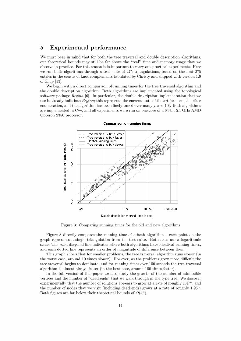
Figure 3: Comparing running times for the old and new algorithms

Figure 3 directly compares the running times for both algorithms: each point on thegraph represents a single triangulation from the test suite. Both axes use a logarithmicscale. The solid diagonal line indicates where both algorithms have identical running times,and each dotted line represents an order of magnitude of difference between them.

This graph shows that for smaller problems, the tree traversal algorithm runs slower (inthe worst case, around 10 times slower). However, as the problems grow more difficult thetree traversal begins to dominate, and for running times over 100 seconds the tree traversalalgorithm is almost always faster (in the best case, around 100 times faster).

In the full version of this paper we also study the growth of the number of admissiblevertices and the number of “dead ends” that we walk through in the type tree. We discoverexperimentally that the number of solutions appears to grow at a rate of roughly 1.47n, andthe number of nodes that we visit (including dead ends) grows at a rate of roughly 1.95n.Both figures are far below their theoretical bounds of O(4n).

11

These small growth rates undoubtedly contribute to the strong performance of the al-gorithm, as seen above. However, our experiments also raise another intriguing possibility,which is that the number of nodes that we visit might be polynomial in the output size. Ifthis were true in general, both the time and space complexity of the tree traversal algorithmwould become worst-case polynomial in the combined input and output size. This would bea significant breakthrough for normal surface enumeration. We return to this speculation inSection 6.

6 Discussion

For topological decision problems that require lengthy normal surface enumerations, weconclude that the tree traversal algorithm is the most promising algorithm amongst thoseknown to date. Not only does it have small time and space complexities in both theory andpractice (though these complexities remain exponential), but it also supports parallelisation,progress tracking, incremental output and early termination. Parallelisation and incrementaloutput in particular offer great potential for normal surface theory.

One aspect of the tree traversal algorithm that has not been discussed in this paper isthe ordering of tetrahedra. By reordering the tetrahedra we can alter which nodes of thetype tree pass the feasibility test, which could potentially have a significant effect on therunning time. Further exploration and experimentation in this area could prove beneficial.

We finish by recalling the suggestion from Section 5 that the total number of nodesvisited—and therefore the overall running time—could be a small polynomial in the com-bined input and output size. Our experimental data (as detailed in the full version of thispaper) suggest a quadratic relationship, and similar experimentation on closed triangula-tions suggests a cubic relationship. Even if we examine triangulations with extremely smalloutput sizes (such as layered lens spaces, where the number of admissible vertices is linear inn [10]), this small polynomial relationship appears to be preserved (for layered lens spaceswe visit O(n3) nodes in total).

Although our algorithm cannot solve the vertex enumeration problem for general poly-topes in polynomial time, there is much contextual information to be gained from normalsurface theory and the quadrilateral constraints. Further research into this polynomial timeconjecture could prove fruitful: a counterexample would be informative, and a proof wouldbe a significant breakthrough for the complexity of decision algorithms in low-dimensionaltopology.

Acknowledgements

The authors are grateful to RMIT University for the use of their high-performance computingfacilities. The first author is supported by the Australian Research Council under theDiscovery Projects funding scheme (project DP1094516).

References

[1] David Avis, A revised implementation of the reverse search vertex enumeration algorithm,Polytopes—Combinatorics and Computation (Oberwolfach, 1997), DMV Sem., vol. 29,Birkhauser, Basel, 2000, pp. 177–198.

[2] David Avis, David Bremner, and Raimund Seidel, How good are convex hull algorithms?,Comput. Geom. 7 (1997), no. 5–6, 265–301.

[3] David Avis and Komei Fukuda, A pivoting algorithm for convex hulls and vertex enumerationof arrangements and polyhedra, Discrete Comput. Geom. 8 (1992), no. 3, 295–313.

12

[4] M. L. Balinski, An algorithm for finding all vertices of convex polyhedral sets, SIAM J. Appl.Math. 9 (1961), no. 1, 72–88.

[5] Joan S. Birman, Problem list: Nonsufficiently large 3-manifolds, Notices Amer. Math. Soc. 27(1980), no. 4, 349.

[6] Benjamin A. Burton, Introducing Regina, the 3-manifold topology software, Experiment. Math.13 (2004), no. 3, 267–272.

[7] , Converting between quadrilateral and standard solution sets in normal surface theory,Algebr. Geom. Topol. 9 (2009), no. 4, 2121–2174.

[8] , The complexity of the normal surface solution space, SCG ’10: Proceedings of theTwenty-Sixth Annual Symposium on Computational Geometry, ACM, 2010, pp. 201–209.

[9] , Extreme cases in normal surface enumeration, In preparation, 2010.

[10] , Optimizing the double description method for normal surface enumeration, Math.Comp. 79 (2010), no. 269, 453–484.

[11] , Maximal admissible faces and asymptotic bounds for the normal surface solution space,J. Combin. Theory Ser. A 118 (2011), no. 4, 1410–1435.

[12] Benjamin A. Burton, J. Hyam Rubinstein, and Stephan Tillmann, The Weber-Seifert dodecahe-dral space is non-Haken, To appear in Trans. Amer. Math. Soc., arXiv:0909.4625, September2009.

[13] David Coulson, Oliver A. Goodman, Craig D. Hodgson, and Walter D. Neumann, Computingarithmetic invariants of 3-manifolds, Experiment. Math. 9 (2000), no. 1, 127–152.

[14] Marc Culler and Nathan Dunfield, FXrays: Extremal ray enumeration software, http://www.math.uic.edu/~t3m/, 2002–2003.

[15] M. E. Dyer, The complexity of vertex enumeration methods, Math. Oper. Res. 8 (1983), no. 3,381–402.

[16] Komei Fukuda, Thomas M. Liebling, and Francois Margot, Analysis of backtrack algorithmsfor listing all vertices and all faces of a convex polyhedron, Comput. Geom. 8 (1997), no. 1,1–12.

[17] Wolfgang Haken, Theorie der Normalflachen, Acta Math. 105 (1961), 245–375.

[18] , Uber das Homoomorphieproblem der 3-Mannigfaltigkeiten. I, Math. Z. 80 (1962), 89–120.

[19] Joel Hass, Jeffrey C. Lagarias, and Nicholas Pippenger, The computational complexity of knotand link problems, J. Assoc. Comput. Mach. 46 (1999), no. 2, 185–211.

[20] William Jaco, The homeomorphism problem: Classification of 3-manifolds, Lecture notes,Available from http://www.math.okstate.edu/~jaco/pekinglectures.htm, 2005.

[21] William Jaco and Ulrich Oertel, An algorithm to decide if a 3-manifold is a Haken manifold,Topology 23 (1984), no. 2, 195–209.

[22] Bruce Kleiner and John Lott, Notes on Perelman’s papers, Geom. Topol. 12 (2008), no. 5,2587–2855.

[23] Hellmuth Kneser, Geschlossene Flachen in dreidimensionalen Mannigfaltigkeiten, Jahres-bericht der Deut. Math. Verein. 38 (1929), 248–260.

[24] Sergei Matveev, Algorithmic topology and classification of 3-manifolds, Algorithms and Com-putation in Mathematics, no. 9, Springer, Berlin, 2003.

[25] T. S. Motzkin, H. Raiffa, G. L. Thompson, and R. M. Thrall, The double description method,Contributions to the Theory of Games, Vol. II (H. W. Kuhn and A. W. Tucker, eds.), Annalsof Mathematics Studies, no. 28, Princeton University Press, Princeton, NJ, 1953, pp. 51–73.

[26] J. Hyam Rubinstein, An algorithm to recognize the 3-sphere, Proceedings of the InternationalCongress of Mathematicians (Zurich, 1994), vol. 1, Birkhauser, 1995, pp. 601–611.

13

[27] Marco Terzer and Jorg Stelling, Parallel extreme ray and pathway computation, Parallel Pro-cessing and Applied Mathematics, Lecture Notes in Comput. Sci., vol. 6068, Springer, Berlin,2010, pp. 300–309.

[28] Jeffrey L. Tollefson, Normal surface Q-theory, Pacific J. Math. 183 (1998), no. 2, 359–374.

[29] Gunter M. Ziegler, Lectures on polytopes, Graduate Texts in Mathematics, no. 152, Springer-Verlag, New York, 1995.

Benjamin A. BurtonSchool of Mathematics and Physics, The University of QueenslandBrisbane QLD 4072, Australia(bab@maths.uq.edu.au)

Melih OzlenSchool of Mathematical and Geospatial Sciences, RMIT UniversityGPO Box 2476V, Melbourne VIC 3001, Australia(melih.ozlen@rmit.edu.au)

14