TR\03\88 July 1988

A TREE SEARCH APPROACH FOR THE SOLUTION OF SET PROBLEMS USING

ALTERNATIVE RELAXATIONS

by

Elia El—Darzi and Gautam Mitra

z1628769

ABSTRACT A number of alternative relaxations for the family of set problems (FSP) in general and set covering problems (SCP) in particular are introduced and discussed. These are (i) Network flow relaxation, (ii) Assignment relaxation, (iii) Shortest route relaxation, (iv) Minimum spanning tree relaxation. A unified tree search method is developed which makes use of these relaxations. Computational experience of processing a collection of test problems is reported. Key words: integer programming, discrete optimisation, set covering, scheduling,

assignment, branch and bound.

CONTENTS 0. Abstract.

1. Introduction to Set Problems(SP).

2. Applications of SP and Test Problems.

3. Preprocessing Heuristics.

4. Alternative Relaxations.

5. A Unified Tree Search Algorithm.

6. Computational Results.

7. References.

8. Appendix.

1. Introductio to set problems(SP)

It has been known that integer programming can represent a wide class of discrete

optimisation problems [DANT 63] and [WILL 85]. In this paper we are interested in a

class of 0-1 integer programming problems: the set covering problem (SCP), the set

partitioning problem (SPP) and together we refer to them as the set problems (SP). They

are well known problems in the field of graph theory and combinatorial optimisation.

It is well accepted that these problems and their solution methods represent most

successful instances of applying discrete models to solve industrial scheduling problems.

Alternative algorithms based on graph theoretic approach for the SP have been investigated

in this paper, using a collection of test problems which were put together to reflect real

life applications.

The contents of this paper is organised as follows. In section 2 applications of the SP are

briefly discussed and the collection of test problems is outlined. In section 3 a few

heuristics which have become established way of preprocessing such problems prior to

applying a full solution algorithms are described. The graph theoretic relaxations which we

introduced constitute a new approach to solving SP and are described in section 4. The

tree search algorithm is described in section 5 and the computational results are presented

in section 6. An example illustrating the relaxations with a small SP model is set out in

Appendix .

Notation and problem definition

Consider a set R={l,2,...,m} and a class H of subsets of R, such that

H= {H1, H2,.....Hn}. Let J={l,2,...,n} be the set of indices for the subsets which make

up the class H.

A cover for R is a subclass of H defined as {Hj|j ∈ Jc} where satisfying ,jccj −

page 1

jcLet.RjHJcj =∈U

be the cost of including Hj in the cover. Thus the minimum

cost set covering problem is that of finding a cover { ∗∈ cJj1jH } as above, such that

∑∗∈ cJj

jc is a minimum.

The SCP may be also posed as a zero-one integer programming problem.

Min (1.1) ∑=

n

1jcjxj

subject to

(1.2) m,....,1in

1j,1aijxj =∑

=>

n,....,1j},1,0{jx =∈ (1.3)

where

⎩⎨⎧

=otherwise0

ercovtheinincludedisjHif1jx

and

⎩⎨⎧ ∈

=otherwise0

jHiif1aij

It is convenient to introduce the index sets Ri, i = l,2,...m, such that for a row i ,

Ri denotes the indices of the columns with unit entry. Similarly, the index sets Hj, j =

l,2,...,n, denote the indices of the rows with unit entry in column j. Thus Hj and Ri

are related to aij: as set out in (1.4) and (1.5)

Hj = {i1aij = 1, i=1.....m) for all j (1.4)

∑=

=m

1iijj aH

and

Ri ={j aij=1, j=1,….,n} for all i׀

(1.5)

page 2

.n

1jijaiR ∑

==

A feasible solution to the SCP is called a cover. A prime cover x*, is a cover for which

xj currently taking value one cannot be reduced to zero without violating a constraint. An

optimal solution to the SCP is a prime cover if all the costs are positive.

The SPP may be defined as

Min (1.6) ∑=

n

1jjxjc

subject to

(1.7) m,....,1i,1xjn

1jjia ==∑

= n,....,1j,}1,0{jx =∈ (1.8) and represents the minimum cost selection such that each member of R is included

exactly once.

2.Applications of SP and test prodlems

It is known that SP represent a wide range of industrial scheduling and planning problems.

These include bus crew scheduling [MTDD 85], air crew scheduling [BAFS 81], vehicle

routing [CHRS 85], steiner problem [FNHT 74], facility location [DKST 81] and others.

For a comprehensive survey on the application of the SP see Balas et al [BLPD 76] and

Balas [BALS 83]. The many applications of the SP have constantly stimulated researchers

to develop new algorithms for the SP. There are many algorithms which solve these

problems. In testing performance of algorithms it is meaningful to use problem instances

which are taken from real or (nearly) real applications. It is doubtful if randomly

generated models have much value in testing algorithms which are designed to solve real

problems. With this in mind we have collected a range of test problems taken from

different contexts which are summarised below. For a full discussion of these models we

page 3

refer the readers to [ELDA 88] and [EDMT 88]. Summary of test problems Table below gives a summary of test problems collected by us.

Problems names

Number of rows

Number of columns

Number of non zero entries

Density

Airline

AIR1 158 416 1371 0.021 AIR2 153 1050 3510 0.022

AIR3 128 1100 3728 0.026 AIR4 148 1100 3670 0.022

AIR5 152 1043 3435 0.021 AIR6 139 1100 3731 0.024

Bus

BUS1 28 231 628 0.097

BUS2 27 168 428 0.094

BUS3 55 1059 3227 0.055

BUS4 53 547 1401 0.048

BUS5 57 31 223 0.126

BUS6 108 245 1538 0.058

BUS7 213 2200 6090 0.013

BUS8 316 3015 12950 0.013

page 4

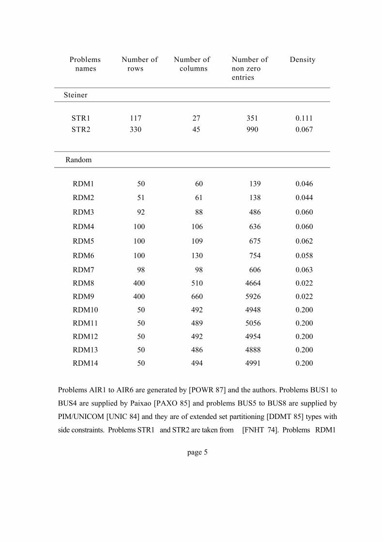
Problems

names Number of

rows Number of

columns Number of non zero entries

Density

Steiner

STR1 117 27 351 0.111 STR2 330 45 990 0.067

Random

RDM1 50 60 139 0.046

RDM2 51 61 138 0.044

RDM3 92 88 486 0.060

RDM4 100 106 636 0.060

RDM5 100 109 675 0.062

RDM6 100 130 754 0.058

RDM7 98 98 606 0.063

RDM8 400 510 4664 0.022

RDM9 400 660 5926 0.022

RDM10 50 492 4948 0.200

RDM11 50 489 5056 0.200

RDM12 50 492 4954 0.200

RDM13 50 486 4888 0.200

RDM14 50 494 4991 0.200 Problems AIR1 to AIR6 are generated by [POWR 87] and the authors. Problems BUS1 to

BUS4 are supplied by Paixao [PAXO 85] and problems BUS5 to BUS8 are supplied by

PIM/UNICOM [UNIC 84] and they are of extended set partitioning [DDMT 85] types with

side constraints. Problems STR1 and STR2 are taken from [FNHT 74]. Problems RDM1

page 5

to RDM14 are supplied by Paixao. They are randomly generated with positive random

costs which vary between 1 and 25 for RDM1 to RDM9 and a cost of 1 for problems

RDM10 to RDM14. All these models are converted to the standard MPSX format using

the modelling system CAMPS [LUMT 87].

3. Preprocessing Heuristics

Preprocessing procedures have been applied by a number of investigators as a preliminary

step towards the solution of large scale SP models [BLHO 80] and [GFNH 72]. These

procedures may be simple algorithms or heuristics and possess computational complexities

which have polynomial time performance. In this section we list a number of procedures

which we have adopted to find tight upper and lower bounds for the SCP and to reduce

the model size. In this composite approach we start by deriving lower and upper bounds

to the SCP using the dual ascent procedure. These bounds are then used as inputs to the

lagrangean relaxation. A sufficient number of subgradient iterations are then applied to

tighten the bounds and to reduce the model size. At the end of the subgradient

optimisation step, the best lagrangean solution is recalled and the row reduction tests are

applied. If some rows are removed from the model by the row reduction tests, the

subgradient procedure is applied again. At this point if an optimal solution to the SCP is

not found we recall the best lagrangean solution already computed and derive a dual

feasible solution. This dual solution is then used to derive the costs of the graph

relaxation models described in section 4.

The composite procedure is made up of four main procedures [ELDA 88] which are

labelled as

(a) dual ascent procedure,

(b) lagrangean and subgradient procedure,

(c) redundant rows procedure

(d) dual solution procedure.

page 6

4. Alternative relaxations

A minimising problem Q is said to be a relaxation of a minimising problem P if the set

of feasible solutions of Q contains the set of all feasible solutions of P and the

corresponding optimal solution value zQ is less than or equal to the optimal solution value

zp. In proposing alternative relaxations to the SP the main motivation is to derive

problems which are easily solved in their relaxed form and provide lower bounds to the

SP. Five graph theoretic relaxations [ELDA 88] have been developed for the SP. These

can be itemised as

- A network relaxation which can be solved by the greedy method,

- An assignment relaxation based on partitioning the constraint set into two

disjoint subsets which represent the set of vertices of the bipartite graph,

- An assignment relaxation using the traveling salesman approach,

- A shortest route relaxation,

- A minimal spanning tree relaxation.

Only the assignment relaxations, the corresponding algorithmic implementation and

computational results are considered in this paper.

A lower bound derived by the assignment 1 representation (ASP1)

Let aj=(a1j,...,amj)T denote the column aj of the SCP problem and let this column be

decomposed into a set of kj columns

)jkja....,,1

ja(

each with at least one unit entry and at most two unit entries. It follows from this

decomposition that

∑=

=jk

1p

pjaja

page 7

The column (nonzero) count of ajp can only be 1 or 2, that is

∑=

=∈m

1ijk,....,1p},2,1{p

ia (4.1)

where {0,1}. ∈pjia

Let q: be the largest positive integer such that qj<( |Hj|+l)/2. The allowable range for kj

is easily seen to be qj<kj<|Hj|. Let the set R (set of rows) be partitioned into two

disjoint sets R' and R" such that R'UR"=R and R'nR" = Φ .

Thus the SCP (1.1-1.3) can be written as

∑=

n

1jjxjcMin (4.2)

subject to

Rin

1j,1jxija ′∈∑

=>

(4.3)

"Ri,n

1j1jxija ∈∑

=> (4.4)

,...,n.1j,}1,0{jx =∈ (4.5)

Introduce two (redundant) constraints indexed m+1 and m+2 such that

0n

1jjxj,1ma∑

=>+ (4.6)

page 8

0jjn

1j,2ma >×

=+∑ (4.7)

Where ⎪⎩

⎪⎨⎧

∈<

′∈=+∑∑

otherwise0Ri

1ijaRi

ijaif1j,1ma 11 (4.8)

and ⎪⎩

⎪⎨⎧

′∈<

∈=+∑∑

otherwise0Ri

1ijaRi

ijaif1j,2ma 11 (4.9)

Thus the SCP can be rewritten as follows

∑=

n

1jjxjcMin (4.10)

subject to

(4.11) Ri,1n

1jjxija ′∈>

=∑

(4.12) 11Ri,1n

1jjxija ∈>

=∑

(4.13) 0n

1jjxj,1ma >

=+∑

(4.14) 0n

1jjxj,2ma >

=+∑

.jallfor}1,0{jx ∈ (4.15)

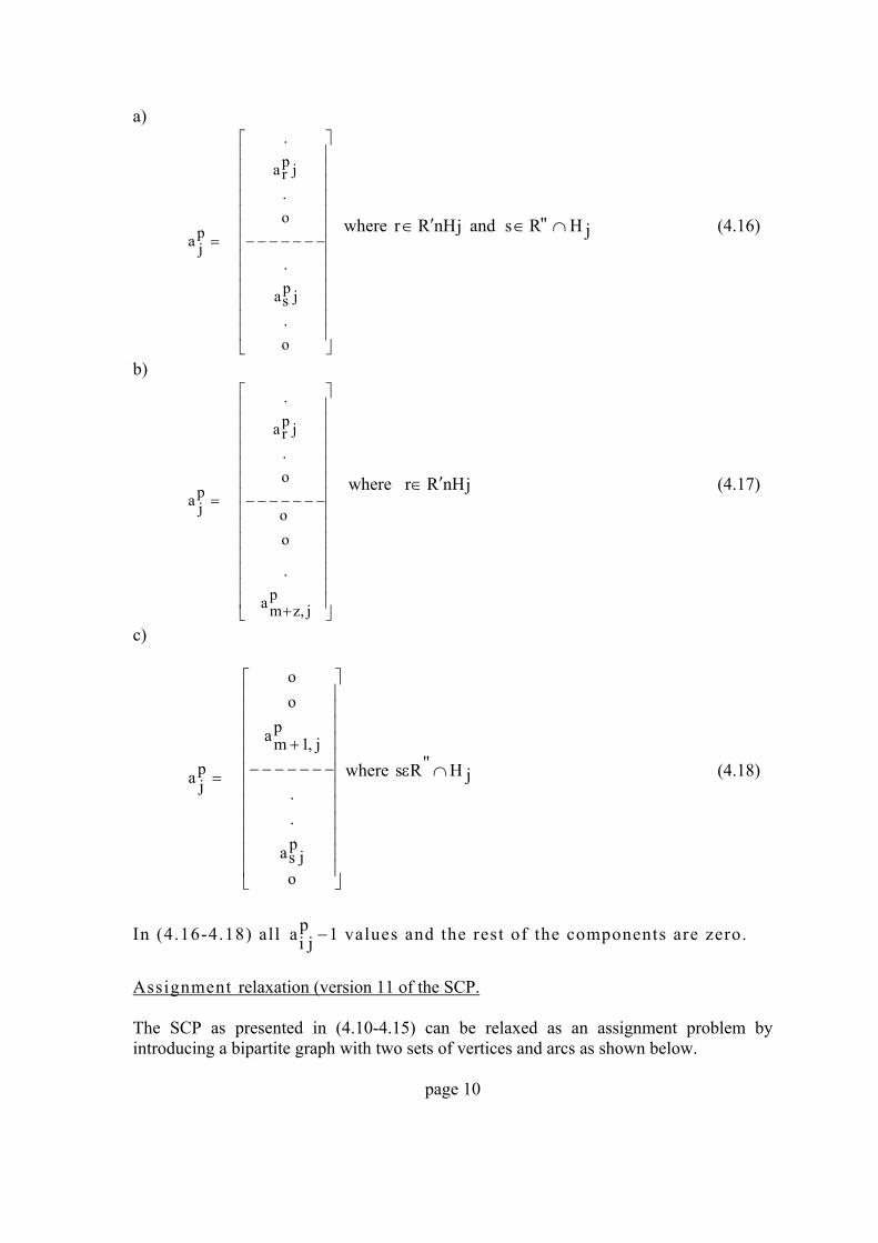
Let R+=R'U{m+l} and R++ = R"U{m+2}. From the definitions set out in (4.1) it follows

that it is always possible to derive a decomposition of aj to

a jp (p=l, . . ,k j) where ap

j takes one of the three alterative forms.

page 9

a)

⎥⎥⎥⎥⎥⎥⎥⎥⎥⎥⎥⎥⎥

⎦

⎤

⎢⎢⎢⎢⎢⎢⎢⎢⎢⎢⎢⎢⎢

⎣

⎡

−−−−−−−=

o.

jpsa

.

o.

jpra

.

pja

where jnHRr ′∈ and (4.16) jH"Rs ∩∈

b)

⎥⎥⎥⎥⎥⎥⎥⎥⎥⎥⎥⎥⎥⎥

⎦

⎤

⎢⎢⎢⎢⎢⎢⎢⎢⎢⎢⎢⎢⎢⎢

⎣

⎡

+

−−−−−−−=

pj,zma

.

oo

o.

jpra

.

pja

where r jnHR′∈ (4.17)

c)

where (4.18)

⎥⎥⎥⎥⎥⎥⎥⎥⎥⎥⎥⎥

⎦

⎤

⎢⎢⎢⎢⎢⎢⎢⎢⎢⎢⎢⎢

⎣

⎡

−−−−−−−+

=

oj

psa

.

.

pj,1ma

oo

pja j

"Rs Η∩ε

In (4.16-4.18) all values and the rest of the components are zero. 1pjia −

Assignment relaxation (version 11 of the SCP. The SCP as presented in (4.10-4.15) can be relaxed as an assignment problem by introducing a bipartite graph with two sets of vertices and arcs as shown below.

page 10

Set of vertices. For the m+2 rows introduce m+2 corresponding vertices 2mv,...,1v + which

are used in the (assignment) graph representation of the problem.

The set of arcs and associated costs. Introduce three sets of arcs

defined as "DAandDA,BA ′

(i) { }"RsandRr/)sv,rv(BA ε′ε=

There is an arc from vr to vs if there exists a column which satisfies pja

(4.16), with the associated cost .1j1/jc2jpd Η−

(ii) { }.Rr\)2mv,rv("D ′ε+−Α

There is an arc from 2m v torv + if there exists a column which satisfies pja

(4.17) with the associated cost .j/jcjpd Η=

(iii) ."Rs)sv,1mv(D ⎭⎬⎫

⎩⎨⎧ ∈+=′Α

T h e r e i s a n a r e f r o m i f t h e r e e x i s t s a c o l u mn wh ich

s a t i s f i e s (4.18). The associated cost is given as

s v to1mv +pja

jpd jH/jcjpd =

Finally introduce an arc set An + 1 with a dummy arc from 1mv + to 2mv + ,

)}2mv,1mv{(1nA ++=+ with zero associated cost 01,1nd =+ , whereby the flow

requirements ( >1) may be imposed on 1mv + and 2mv + . Let denote the

corresponding dummy column. Let A denote the directed arcs of the resulting graph such

that A={

1na +

1nA"DDBA +Α′Α UUU }. Figure 4.1 illustrates the structure of this graph. Let

denote the set of arcs obtained by decomposing the column j in the manner indicated

earlier. Thus there are arcs in , where for (v

jA

jk jA r,vs) ,jA∈ +∈Rrv and ++∈Rrv as

explained in (4.16-4.18). It is easy to see that

U1n

1j.AjA

+

==

page 11

Figure 4.1

A statement of the relaxed problem [FRZE 85]. With each column associate

a variable and a cost coefficient d

ja

}1,0{jpy,jpy ∈ jp which are defined for j=l,...,n+l and

. Then the relaxed problem ASP1 is stated as jk,....,1p =

Min (4.19) ∑ ∑+

= =

1n

1j

jk

1pjpyjpd

subject to

(4.20) ∑ ∑+

= =

+∈>α1n

1j

jk

1pRr,1jpyp

jsr

(4.21) ∑ ∑+

= =

+ε>α1n

1j

jk

1pRs,1jpyp

jsr

page 12

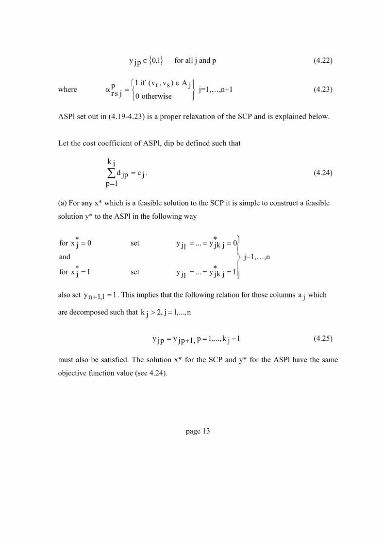
for all j and p (4.22) { }1,0pjy ∈

where j=1,…,n+1 (4.23) ⎭⎬⎫

⎩⎨⎧ ε

=αotherwise0

jA)sv,rv(if1pjsr

ASPl set out in (4.19-4.23) is a proper relaxation of the SCP and is explained below. Let the cost coefficient of ASPl, dip be defined such that

(4.24) ∑=

=jk

1p.jcjpd

(a) For any x* which is a feasible solution to the SCP it is simple to construct a feasible

solution y* to the ASPl in the following way

⎪⎪⎭

⎪⎪⎬

⎫

====

====

1*jjky...1jyset 1*

jxfor

and

0*jjky...1jyset 0*

jxfor

j=1,…,n

also set . This implies that the following relation for those columns which

are decomposed such that

11,1ny =+ ja

n,...,1j,2jk =>

1jk,...,1p,1pjypjy −=+= (4.25) must also be satisfied. The solution x* for the SCP and y* for the ASPl have the same

objective function value (see 4.24).

page 13

(b) If the optimal solution y to the ASPl also satisfies (4.25) then this implies that the

vector x computed by the relations

−−= jpyjx j=1,..,n, p=1,…,kj (4.26)

is also an optimum solution to the SCP. If the optimal solution to the ASPl does not

satisfy (4.25) it still provides a valid lower bound on the optimal objective value of the

SCP. At this stage a tree search method can be used to satisfy the relations (4.25) by

suitably fixing groups of yjp to zero or one.

Let ),jjk,...,1j(j λλ=λ j=1,…,n represent the lagrangean multipliers

associated with the side constraints of the decomposed column (j=l,...,n) where ja jλ are

unrestricted in sign. Let )n,...,1( λλ=λ represent a collection of lagrangean multipliers

The lagrangean relaxation [GOEF 74] LASPl(λ ) of the ASPl as set out in (4.19-4.23) and

(4.25) can be written as

Min ∑=

∑=

−λ−λ+n

1j

jk

1k)1jkjkjkd(kjy

subject to

network constraints (4.20-4.21)

and

jk,...,1kandn,...,1j},1,0{kjy ==∈

where n,...,1j,0jjkojy ==λ=

If we replace the inequality (">") in (4.20) and (4.21) by equality ("=") for Rr ′∈ and

respectively then the modified ASPl becomes a relaxation to the SPP. This implies

that the constraints corresponding to i

"Rs∈

ε R must be strictly equal to 1, while the two

constraints corresponding to iε {m+l,m+2} can be > 1.

page 14

A lower bound derived by the assignment 2 representation (ASP2)

Let kj = jH denote the number of 1's in the column Let as defined

i n ( 1 . 4 ) b e r e - e x p r e s s e d a s H

ja jH

j = { }jki,...,1i . I n t roduce t he ve r t ex s e t V

corresponding to the rows i=l,...,m of the SCP such that V={v,,...,vm}. For each column

aj construct a set of kj directed arcs from V to V which admit unit flow in the following

way. The arc sets in the equivelent bipartite graph are denoted by Aj where

A j = , j = 1 , … , n (4.27) ⎭⎬⎫

⎩⎨⎧

−)1iv,

jkiv(,)jkiv,1jkiv(,...,)3iv,2iv(,)2iv,1iv(

Let the associated cost for each arc in the arc set Aj be defined as (4.28) .jk/jcjd =

With each of the arcs taken from the set associate a var iable

{0,1} and defined for all (v

jk jA

∈jpqy p,vq) jA∈ . (4.29)

Let j=1,…,n (4.30) ⎭⎬⎫

⎩⎨⎧ ε

=αotherwise0

jA)qv,pv(if1jpq

The r e l axed p rob l em ASP2 i s s t a t ed a s f o l l ows .

Min (4.31)

∑=

∑ε

n

1j jA)qv,pv(

jpqyjd

subject to

(4.32) ∑=

=>αn

1jm,...,1i,1j

qiyjqi

(4.33) ∑=

=>αn

1jm,...,1i,1j

ipyjip

page 15

(4.34) jA)qv,pv(andn,...,1j,}1,0{jpqy ε=ε

ASP2 set out in (4.31-4.44) is a proper relaxation of the SCP. This is explained below. (a) for any x* which is a feasible solution to the SCP it is simple to construct a feasible

solution y* to the ASP2 by the procedure

⎪⎪⎭

⎪⎪⎬

⎫

ε==

ε==

jA)qv,pv(,1j*pqyset1*

jxfor

andjA)qv,pv(,0j*

pqyset0*jxfor

j=1,…,n

This implies that the following relations for those columns aj such that ,2jH > j=l,...,n

j

1ijkiy...j

3i2iyj

2i1iy === (4.35)

must also be satisfied. The feasible solution y* to the ASP2 has a cost which is equal to

the cost of the feasible solution x* of the SCP (see 4.28).

(b) If the optimal solution y to the ASP2 also satisfies (4.35) then this implies that the

vector x computed by the relations

jAε)qv,p(vandn1,...,j,jpqyjx == (4.36)

is also an optimum solution to the SCP. If the optimal solution to the ASP2 does not

satisfy (4.35), it still provides a valid lower bound on the optimal objective value of the

SCP. At this stage a tree search method can be used to satisfy the relations (4.35) by

page 16

suitably fixing groups of kj variables as defined in (4.35) to the values zero or one.

L e t ),jkj,...,1j(j λλ=λ j = 1 , … , n r e p r e s e n t t h e l a g r a n g e a n m u l t i p l i e r s

associated with the side constraints of the decomposed column aj (j=l,...,n) where are

unrestricted in sign. Let

jλ

)n,...,1( λλ=λ represent a collection of lagrangean multipliers

The lagrangean relaxation [GOEF 74] LASP2(λ ) of the ASP2 as set out in (4.31-4.34)

and (4.35) can be written as

Min )1jkjkj

1kikid(j

1kikiy

n

1j

jk

1k−λ−λ+

++∑=

∑=

subject to

network constraints (4.32-4.33)

and

jA)qv,pv(andn,...,1j,}1,0{jpqy ε=ε

where .n,...,1j,1i1jki,0jjkoj ==+=λ=λ

If we replace the inequality ">" in (4.32-4.33) by equality "="H then the modified ASP2

becomes a relaxation to the SPP.

5. A unified tree search algorithm

Branch and bound is one of the most successful techniques for solving combinatorial

optimisation problems, covering discrete optimisation models in general and integer

programming problems in particular [MRTY 76]. The computational efficiency of the tree

developement and the search procedure which follows from branch and bound depends on

a number of factors which are considered below.

In designing the branch and bound algorithm, we wish to control the size of the tree

page 17

developed and the process of searching for the optimal solution of the original problem,

that is, controlling the number of subproblems proposed. This search strategy depends on

the heuristics as defined by the choices made at the following algorithmic steps.

(a) The type of the relaxation used to represent the original problem (problem

representation). This also influences the time taken to solve each subproblem

(reoptimise).

(b) The choice of the branching variable (branching strategy).

(c) The choice of the best subproblem to solve (search strategy).

In this context Breu et al [BRBD 74] have surveyed the art and science of branch and

bound techniques for 0-1 integer programming. Shapiro [SHAP 79] has incorporated the

lagrangean relaxation within the framework of the tree search procedure and Mitra

[MTRA 73] has investigated different strategies for the tree search procedure as applied to

mixed integer programming.

To start with one of the relaxed SCP problems, namely, ASP1 or ASP2 is solved at the

root node. After solving the subproblem the solution is analysed and a variable is chosen

for branching. The choice of a branching variable is a difficult task and no universal rule

exists which gives a uniformly good result. Many investigators have remarked that, this

choice rule should be formulated by studying the problem and its structure. By and large

good branching rules are highly context dependent. In choosing the next subproblem from

the waiting list of subproblems held in a stack, again many alternative criteria can be used

and together with the variable choice strategies, these determine the size of the search

tree. In our investigation we have taken the most popular method of last in first out

(UFO) rule.

page 18

An outline of the unified tree search strategy

The alternative strategies which are adopted in the design of the branch and bound

procedure are outlined in the statement of the algorithm set out below. At each step of

the solution process it is necessary to know whether or not a feasible solution to the SCP

is obtained. It is also necessary to know the value of the best objective function which is

denoted by zmin. Also we use to denote the optimal solution value of the relaxed

problem (ASP1 or ASP2), that is, a lower bound on the objective function value of the

SCP. Before stating the algorithm we explain how the search is terminated at each branch

of the tree depending on the outcome of the subproblem investigation. A node is

fathomed if after the solution of the subproblem one of the following conditions hold.

lz

(1) The lower bound is greater than the upper bound.

(2) The subproblem has no feasible solution.

(3) The optimal solution to the relaxed problem is found and this also satisfies the side

contraints. Hence it is a feasible solution to the SCP and because of (1) above it is also

the best feasible solution to the SCP found so far.

Step(l) Preprocessing procedure

In this step the composite preprocessing procedures (a), (b) and (c) outlined in

section 3 are applied to reduce the model size and to derive an upper bound

( minz ) and a lower bound (z ) on l z . If lz > minz - 1 go to Step(11),

otherwise apply the preprocessing procedure (d) to obtain a dual feasible

solution, which is used to derive the cost vector of the relaxed problem.

Step(2) Solution at the root node

The relaxed SCP problem is solved at the root node of the tree. If lz >

minz - 1 or the side constraints are satisfied go to Step(11), (the optimal

solution to the SCP is obtained which is equal to minz in the former and

in the latter), else initialise the lagrangean multipliers and go to Step(8).

lz

Step(3) Choice of the branching variable(s)

Select a group of network variables yjk corresponding to the arcs in the arc set

page 19

Aj for branching. Add the two subproblems with

and to the list of subproblems, store their positions in the list

and go to Step(4b).

)jk,...,1k,1jky( ==

)jk,...,1k,1jky( ==

Step(4) Subproblem selection

(a) If the list of subproblems is empty go to Step(11).

(b) Choose a subproblem from the list.

Step(5) Subproblem preparation

Prepare the subproblem to be optimised, that is, identify the out-of- kilter

arcs, for example, update the list of subproblems, etc.

Step(6) Subproblem solution

Solve the subproblem using a network optimiser [FDFL 62].

Step(7) Subproblem solution analysis

If the subproblem has no feasible solution or the objective solution value is

greater than Zmin -1 then go to Step(4). If the side constraints are satisfied go

to Step(10). Otherwise go to Step(8).

Step(8) Solution improvement and model reduction

Test for optimal network solution improvement. Temporary remove the

redundant columns using reduced cost analysis and single row tests.

Step(9) Lagrangean and subgradient procedure

If the number of subgradient iterations exceed an iteration counter (LMAX) go

to Step(3). Otherwise compute the lagrangean multipliers, update the

corresponding costs, set the negative costs to nonnegative costs and go to

step(5).

Step(10) Update the best SCP solution

A feasible solution to the SCP has been found. Update minz and the

corresponding solution vector and go to Step(4).

Step(11) SCP optimal solution

Output the best SCP feasible solution and the corresponding optimal objective

value ( minz ).

page 20

6. Computational results

The computational results to the branch and bound algorithm designed for the ASP1 and

ASP2 are given in tables 6.1 and 6.2 respectively. This algorithm is applied to the test

problems which have not been optimaly solved using the preprocessing procedures of

section 3. The abbreviations used in these tables headings are explained below.

z is the optimal solution value if found. A value with a "*" represents the best feasible

solution found within the time limit.

m, n are the reduced dimensions of the test problems, where m denotes the number of

rows and n denotes the number of columns.

uz is the best upper bound derived using the preprocessing procedures. The computing

time taken of the preprocessing procedures is given in the next column. The bound

derived by the ASP1 and ASP2 at the root node of the tree and the corresponding

computing time are also reported in these tables, followed by the total number of nodes

developed in the process of searching for the optimal solution. The number of lagrangean

iterations applied within the framwork of the tree search is also tabulated. The last two

columns in these tables represent the total time for the branch and bound algorithm (not

including step(l)) and the total execution time. The maximum running time permitted was

set to 1000 cpu seconds.

page 21

Computational results of processing the test problems by the tree search method on ASP1.

Table 6.1

All times are in seconds of Honeywell Multics DP6840 processing

PREPRO- INITIAL NO OF

PROBLEM

REDUCED DIMENSIONS

CESSING NETWORK NO OF LAG B&

NAME Z m n uz TIME SOLUTION TIME NODES ITER TIM

AIR1 16635 120 297 16660 40.93 16577.2 6.12 1136 601 95

B TOTAL

E TIME

4.1 995.0

AIR2 18880 129 436 18885 269.3 18833.1 7.3 26 11 67

AIR3 18195 104 499 18195 175.4 18124.0 6.9 145 113 52

AIR4 19715 138 1089 19795 100.9 19462.7 16.57 225 144 19

AIR5 21560 131 1003 21800 104.55 21377.3 14.67 357 173 34

AIR6 16925 124 998 17000 124.3 16795.0 14.55 31 0 44

BUS2 41051 26 90 41537 1.52 41036.4 .04 16 2

BUS3 64749* 55 977 64749 62.31 63000.2 7.6 487 539 >100

BUS4 74787* 53 547 75212 26.63 72086.1 2.6 818 966 >100

RIM4 97 99 74 97 11.5 93.23 .21 75 30 45

RIM5 96 31 54 96 10.7 94.37 .12 37 30 34

RIM6 87 57 40 87 15.2 85.6 .59 70 31 1

.0 336.3

8.3 703.7

7.9 298.8

2.7 347.2

.1 168.4

.87 2.39

0 >1000

0 >1000

.4 56.9

.8 45.5

6.3 31.5

page 22

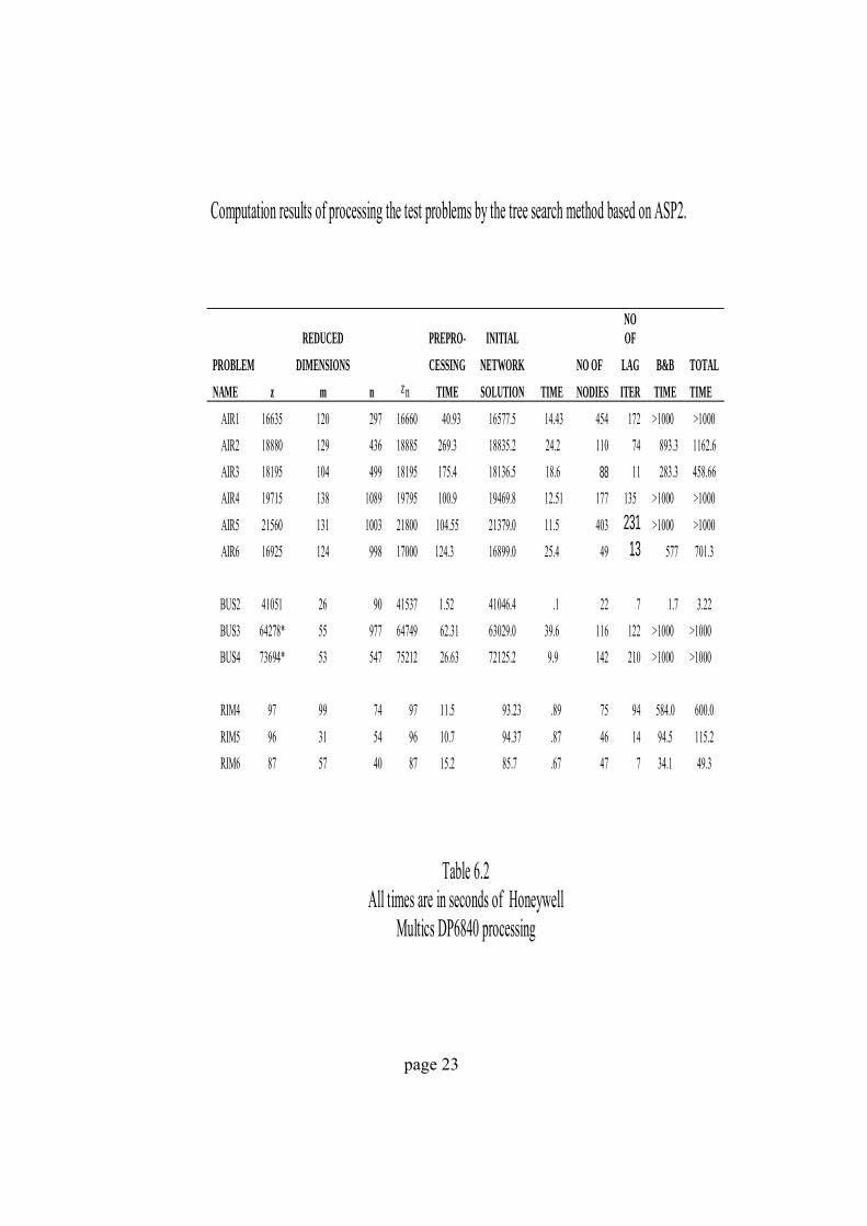
Computation results of processing the test problems by the tree search method based on ASP2.

Table 6.2 All times are in seconds of Honeywell

Multics DP6840 processing

REDUCED PREPRO- INITIAL NO OF

PROBLEM DIMENSIONS CESSING NETWORK NO OF LAGNAME z m n nz TIME SOLUTION TIME NODIES ITER

AIR1 16635 120 297 16660 40.93 16577.5 14.43 454 172

B&B TOTAL TIME TIME

>1000 >1000 AIR2 18880 129 436 18885 269.3 18835.2 24.2 110 74 AIR3 18195 104 499 18195 175.4 18136.5 18.6 88 AIR4 19715 138 1089 19795 100.9 19469.8 12.51 177 135 AIR5 21560 131 1003 21800 104.55 21379.0 11.5 403 231 AIR6 16925 124 998 17000 124.3 16899.0 25.4 49 13

BUS2 41051 26 90 41537 1.52 41046.4 .1 22 7 BUS3 64278* 55 977 64749 62.31 63029.0 39.6 116 122 BUS4 73694* 53 547 75212 26.63 72125.2 9.9 142 210

RIM4 97 99 74 97 11.5 93.23 .89 75 94 RIM5 96 31 54 96 10.7 94.37 .87 46 14 RIM6 87 57 40 87 15.2 85.7 .67 47 7

893.3 1162.6 11 283.3 458.66

>1000 >1000 >1000 >1000

577 701.3

1.7 3.22 >1000 >1000 >1000 >1000 584.0 600.0 94.5 115.2 34.1 49.3

page 23

The ASP1 solved nearly all the test problems within the time limit, except for BUS3 and

BUS4. The ASP2 fails to solve problems AIR1, AIR4, AIRS, BUS3 and BUS4 within this

time limit. The lagrangean and subgradient procedures manage to improve the bounds at

the lower levels of the tree, that is, when a large number of variables have been fixed to

either one or zero, but, at the expense very high computing time. The best feasible

solutions obtained for BUS3 and BUS4 test problems by the ASP2 are better than these

obtained by the ASP1.

Overall more experiments are needed to "successfully" incorporate the lagrangean and

subgradient procedures within the tree search procedure. Different branching strategies also

may be worth investigating and of course a faster network optimiser will improve the

performance of this algorithm.

page 24

REFERENCES

[BAFS 81] Baker, E., and Fisher, M., "Computational results for very large air crew

scheduling problems", Omega, 9, pp613-618, (1981)

[BALS 83] Balas, E., "A class of location, distribution and scheduling problems: modelling

and solution methods". Revue Beige de Statistique, d'Informatique et de Recherche

Operationnelle, 22, pp36-57, (1983)

[BLHO 80] Balas, E., and Ho, A., "Set covering algorithms using cutting planes,

heuristics and subgradient optimization: A new computational study", Mathematical

Programming Study, 12, pp37-60, (1980)

[BLPD 76] Balas, E., and Padberg, M.W., "Set partioning: A survey", SIAM Review, 18,

pp710-760, (1976)

[BRBD 74] Breu, R., and Burdet, C.A., "Branch and bound experiments in 0-1

programming", Mathematical Programming Study, 2, ppl-50, (1974)

[CHRS 85] Christofides, N., "Vehicle routing" in "Travelling salesman problem", Lawler,

E.L., Lenstra, J.K., Rinooy Khan, A.H.G., and Shmays, D.S., eds, Academic Press,

(1985)

[DANT 63] Dantzig, G., "Linear programming and extensions", Princeton University Press,

Princeton, New Jersey, (1963)

page 25

[DDMT 85] Darby-Dowman, K., and Mitra, G., "An extension to set partitioning with

application to scheduling problems", European Journal of Operations Research, 21,

pp200-205, (1985)

[DKST 81] Dasltin, M.S., and Stern, E.D., "A hierarchical objective set covering model

for emergency medical service vehicle deployment" Transportation Science, 15, ppl37-152,

(1981)

[EDMT 88] E, El-Darzi., and G, Mitra., "Set covering and set partitioning: A collection

of test problems", Brunei University, Internal Report, (1988)

[ELDA 88] E, El-Darzi., "Methods for solving the set covering and set partitioning

problems using graph theoretic (relaxation) algorithms", Brunei University, PhD thesis,

(1988)

[FDFL 62] Ford, L., and Fulkerson, D., "flows in networks", Princeton University Press,

(1962)

[FNHT 74] Fulkerson, D.R., Nemhauser, G.L., and Trotter, L.E., "Two computationally

difficult set covering problems that arises in computing the 1-Width of incidence matrices

of steiner triple systems", Mathematical programming Study, 2, pp72-81, (1974)

[FRZE 85] Frieze, A., "Private communication", (1985)

[GEOF 74] Geoffrion, A.M., "Lagrangean relaxation for integer programming",

Mathematical Programming Study, 2, pp82-114, (1974)

[GFNH 72] Garfinkel, R.S., and Nemhauser, G.L., "Integer programming", Wiley, (1972)

page 26

[LUMT 87] Lucas, C, and Mitra, G., "Computer assisted mathematical programming

modelling system (CAMPS)” User Specification, Brunei University, Department of

Mathematics and Statistics, (1987)

[MRTY 76] Murty, K.G., "Linear and combinatorial programming", John Wiley and Sons,

(1976)

[MTDD 85] Mitra, G., and Darby-Dowman, K., "CRU-SCHED A computer based bus

crew scheduling system using integer programming", in "Computer scheduling of public

transport", Rousseau, J.-M., Ed., North Holland, (1985)

[MTRA 73] Mitra, G., "Investigation of some branch and bound strategies for the solution

of mixed integer linear programs", Mathematical Programming, 4, ppl50-170, (1973)

[PAXO 85] Paixao, J., "Private communication", (1985)

[POWR 87] Powers, D., "Investigation and construction of set covering and set partitioning

test problems", BSc dissertation, Brunei University, (1987)

[SHAP 79] Shapiro, J.F., "A survey of lagrangean techniques for discrete optimization",

Annals of Discrete Mathematics, 5, pp113-138, (1979)

[UNIC 84] "Private communication", Unicom Consultancy, Brunei Science Park, (1984)

[WILL 85] Williams, H.P., "Model building in mathematical programming", John Wiley

and Sons, (1985)

page 27

Appendix

ILLUSTRATIVE EXAMPLE OF THE ALTERNATIVE RELAXATIONS

In this appendix the alternative relaxations of the SP (ASPl, ASP2) are illustrated .using the SCP example set out in the tableau below. variables. yjk,k=l,...kj reprsent the variables for the assignment relaxations, where kj denotes the total number of arcs derived from column a: of the SCP.

c c c c c c c c 0 0 0 0 0 0 0 0 1 1 1 1 1 1 1 1 1 2 3 4 5 6 7 8

cost 4 3 3 2 3 2 3 4

row1 1 1 1 1 > 1

row2 1 1 1 1 > 1

row3 1 > 1

row4 1 1 > 1

row5 1 1 1 > 1

row6 1 1 > 1

row7 1 1 > 1

row8 1 1 > 1

Page 28

The ASP1 representation of the SCP example

page 29

The ASP2 representation of the SCP example