LUND UNIVERSITY

PO Box 117221 00 Lund+46 46-222 00 00

A Tool for Utility Disturbance Management

Lindholm, Anna; Johnsson, Charlotta

Published in:14th IFAC Symposium on Information Control Problems in Manufacturing

2012

Link to publication

Citation for published version (APA):Lindholm, A., & Johnsson, C. (2012). A Tool for Utility Disturbance Management. In 14th IFAC Symposium onInformation Control Problems in Manufacturing IFAC.

Total number of authors:2

General rightsUnless other specific re-use rights are stated the following general rights apply:Copyright and moral rights for the publications made accessible in the public portal are retained by the authorsand/or other copyright owners and it is a condition of accessing publications that users recognise and abide by thelegal requirements associated with these rights. • Users may download and print one copy of any publication from the public portal for the purpose of private studyor research. • You may not further distribute the material or use it for any profit-making activity or commercial gain • You may freely distribute the URL identifying the publication in the public portal

Read more about Creative commons licenses: https://creativecommons.org/licenses/Take down policyIf you believe that this document breaches copyright please contact us providing details, and we will removeaccess to the work immediately and investigate your claim.

A Tool for Utility Disturbance

Management

Anna Lindholm ∗ Charlotta Johnsson ∗

∗ Department of Automatic Control, Lund University, Sweden(e-mail: anna.lindholm@control.lth.se).

Abstract: Disturbances in the supply of utilities may lead to large economical losses atindustrial sites. In order to take appropriate decisions on for which utilities improvement effortsshould be made, a tool for evaluating the economical effects of utility disturbances is needed.This paper presents a tool for quickly estimating the revenue loss caused by each utility, usingsimple matrix operations. A matrix representation of a site is introduced to be able to quickly getkey performance indicators for any site. The revenue loss is estimated using an on/off productionmodeling approach.

Keywords: Disturbance management, Performance evaluation, Enterprise modeling, Utilities,Process control, Decision support systems, Data processing

1. INTRODUCTION

Process industrial sites are often complex, and model-ing such sites in detail is often both hard and time-consuming (Niebert and Yovine (1999)). In situationswhere quick decisions must be taken, there is often nottime for detailed modeling. For such situations, key perfor-mance indicators (KPIs) can be used for decision support,for example at decisions on where to focus maintenanceefforts or include more redundancy. One decision supportframework that utilizes KPIs for disruption managementin the supply chain is presented in Bansal et al. (2005).

In this study, the focus is on disturbances in utilities, suchas steam and cooling water. These disturbances are oftenplant-wide disturbances that affect several production ar-eas at a site, which makes their impact on production hardto predict. Lindholm et al. (2011b) presented a generalmethod for reducing the economical effects of disturbancesin utilities. This method was applied to an industrial site inLindholm et al. (2011a) using an on/off production model-ing approach. In the present study, a matrix representationof a site and its utilities is introduced, that simplifies useof the method in Lindholm et al. (2011b). Performaceindicators such as utility and area availability are easilycalculated, and the revenue loss caused by each utility isestimated via the on/off production modeling approach.A general tool for proactive disturbance management ispresented, that can efficiently be applied to any processindustrial site, since it utilizes the general matrix represen-tation. The case study in Lindholm et al. (2011a) is redoneusing this new utility disturbance management tool, toshow the usefulness of the representation framework.

2. PHYSICAL HIERARCHY OF AN ENTERPRISE

According to the role based equipment hierarchy defined inthe standard ISA-95.00.01 (2009), an enterprise containsone or more sites, which in turn consist of one or moreareas. Each production area has one or more production

units and each production unit consists of one or moreunits.

The enterprise determines which products to manufactureand at which site they should be produced. Sites areusually geographically grouped, and are used for rough-cut planning and scheduling. Areas are usually groupedby their geographic location and by their products. Eacharea produces one or more products, either end productsfor external sale or intermediates for further use by otherareas at the site. Production units generally include allequipment required for a segment of continuous produc-tion. A production unit in the process industry could bee.g. a reactor or a distillation column. Units are composedof lower level equipment, such as sensors and actuators.

For application of a general disturbance managementmethod, a conveninent way of representing a site is needed.Usually, a flowchart is available at a site, that depicts theareas of the site and the product flow through these areas.Using the flowchart, a matrix representation of the sitecan easily be produced. How this is done is discussed inSection 7.

3. UTILITIES

Utilities are support processes that are utilized in pro-duction, but are not part of the final product. Utilitiesmay be seen as belonging to the ’Material’ category inthe standard ISA-95.00.01 (2009). Common utilities withinthe process industry are e.g. steam, cooling water andelectricity. For a more complete list, see e.g. Brennan(1998) or Lindholm et al. (2011b).

Utilities are often such that they only affect productionwhen their supply is interrupted or does not meet thespecifications. In Lindholm et al. (2011b), disturbances inthe supply of utilities are defined as when the measurementof a utility parameter, such as temperature or pressure,goes outside a limit at which the poor operation of theutility will have negative consequences for the production

T-122

at the site. One utility may be affected by several utilityparameters, for example both flow and temperature of theutility. The disturbance limits may be set using knowledgeof personnel at a site or may be estimated using measure-ment data.

4. DISTURBANCE MANAGEMENT

Two main approaches of disturbance management couldbe identified, disturbance handling at the occurrence ofa disturbance, and preventive disturbance managementstrategies that aim to reduce the number of disturbances.These two approaches have been given different nameswithin different research areas, and are sometimes alsodivided into sub-approaches. Here the terms reactive andproactive disturbance management are used. These termsare also used in Barroso et al. (2010), where they are de-fined for the supply chain, and in Monostori et al. (1998),where they are used in the context of scheduling. Theformal definitions of reactive and proactive disturbancemanagement that are used in this paper are given below.

proactive disturbance management —disturbance management strategies that are aimingto prevent future disturbance occurrences.

reactive disturbance management —disturbance management strategies for handling dis-turbances when they occur.

The tool that is introduced in this paper can be used forproactive disturbance management.

5. PERFORMANCE INDICATORS

5.1 Utility Availability

The availability of a production unit is according to thestandard ISO/WD-22400-2 (2011) the ratio between theactual production time and the planned allocation time,where the planned allocation time is the time in which theunit can be used (the operation time) minus the planneddowntime. For utilities, availability is defined in Lindholmet al. (2011b) as the fraction of time all utility parametersare inside their limits. This represents the fraction oftime when there is a possibility for maximum production,assuming that all utility disturbance limits have beencorrectly set. This means that a utility is available whenall its utility parameters are inside their limits, and notavailable otherwise. Utility availability can be computedif measurements of all utility parameters are available.Planned stops should not be included in the availabilitycomputations. Calculation of utility availabilities using amatrix representation of a site and its utilities is handledin Section 7.2.

Utility dependence Some utilities are dependent on otherutilities, which may have as consequence that a distur-bance in one utility also shows up in the measurements ofother utilities. For example, if feed water is not available,steam could not be produced, and the steam utility couldnot possibly be available. This should be considered a feedwater failure and not a steam failure, since feed water

is the root cause of the disturbance. Utility dependencecan be represented in a flowchart. An example of a utilitydependence flowchart is given in the example in Section 8.

Utility dependence can be taken into account when calcu-lating utility availability. If it is not taken into account, theutilities dependent on other utilities will appear to havelower availability than they actually have. Calculation ofutility availability when taking utility dependence intoaccount is handled in Section 7.2.

In some cases, interdependency between utilities mightoccur. An example is the reliance of water distributionon electricity, and simultaneous reliance of electricity gen-eration on water. This would appear as loops in the utilitydependence flowchart. The computational framework pre-sented in Section 7.2 can currently not handle this. Thereason is that the root cause of the disturbance has tobe determined, which is impossible if only considering onesample point in utility measurement data. One solution tothe problem is to, if possible, divide the considered utilitiesinto sub-utilities to get rid of the loops in the utilitydependence flowchart. Another solution is to consider theorder in which the failures show up in measurement datato determine the root cause of each disturbance.

5.2 Area Availability

A simple estimate of the availability of each area, withrespect to utilities, is the fraction of time all utilitiesneeded at the area are available; i.e. the intersection ofthe operation of all concerned utilities. The measure ofarea availability should be interpreted as the fraction oftime an area has the possibility of operating at maximumproduction rate, with respect to utilities. Area availabilitycomputed without considering the connection of areas ata site is denoted direct area availability.

Area dependence If an area is unavailable, this mayalso affect other areas at the site, since areas could bedependent on obtaining raw materials from, or deliveringproduct to, other areas. The area interdependence can beseen in a flowchart of the product flow at the site.

To include area dependence in the measure of area avail-ability, total area availability is introduced. Total areaavailability is defined as the fraction of time all the re-quired utilities, and all areas that the area is dependent on,are available. Thus, total area availability contains boththe direct effects of a utility disturbance, and the indirecteffects because of area dependence. Computation of bothdirect and total area availability using matrices is handledin Section 7.3.

5.3 Production Revenue Loss

Production revenue loss is obtained when an area cannotoperate at the desired production rate. The revenue lossis here defined as the contribution margin multiplied bythe duration when production was reduced, and by thedifference of the desired production rate and the actualproduction rate during the time period. The contributionmargin is the marginal profit per volume.

Here, maximum production is considered to be the desiredproduction rate, since this is how the utility disturbance

T-123

limits are defined. The flows to the market of the productsof the site at maximum (steady-state) production are usedto estimate the revenue loss. For an area, the direct revenueloss is the loss of revenue due to poor operation of theutilities at that area. The total revenue loss is obtainedif also the effects of utility disturbances in areas that thearea is dependent on are considered. For utilities, the directrevenue loss is the loss each utility causes directly, becauseof reduced production in the areas that require the utility.The total revenue loss also includes the revenue loss dueto reduced production in areas that are dependent on theareas that require the utility.

An estimate of the production revenue loss due to dis-turbances in utilities can quickly be obtained using anon/off production model of the site. The computationsmay be performed with matrices, as described in Section 7.On/off production modeling is described in Section 6. Ifthe desired production rate varies during the time periodthat is considered, the period may be divided into intervalsfor which the desired production rate is constant. Anestimate of the revenue loss for the entire time period isthen obtained by summarizing the partial estimates.

6. ESTIMATION OF REVENUE LOSS

6.1 On/Off Production Modeling

The on/off production model is the simplest way of mod-eling the effect of utility disturbances on production. Withthis modeling approach, utilities and areas are consideredto be either operating or not operating, i.e. ’on’ or ’off’. Anarea operates at maximum production speed when all itsrequired utilities are available, and does not operate whenany of its required utilities is unavailable. It is assumedthat there are no buffer tanks between the areas at thesite. This means that if an area is unavailable, the areasdownstream with respect to the product flow will also beunavailable. The on/off model does not adequately reflecthow the actual production is managed for most sites,but is because of its simplicity useful for obtaining quickestimates of production losses due to disturbances. The es-timates can be used to help identifying which disturbancesthat have the greatest economical effects.

6.2 Estimation of Revenue Loss using On/Off Modeling

Estimation of Revenue Loss for each Product Withon/off production modeling without buffer tanks, areas areassumed to be operating at maximum production speedwhen available, and not at all when not available. Thus,the direct and total area availabilities may be used to esti-mate the direct and total revenue loss for each product dueto all disturbances in utilities. The area availabilities andthe flows to the market at maximum production are usedto compute the production losses, which are translatedinto revenue losses using the contribution margins of theproducts. The computations can be done efficiently withmatrices, see Section 7.4.

Estimation of Revenue Loss due to each Utility Foron/off production modeling without buffer tanks, the util-ity availabilities may be used to estimate the direct and

total revenue loss caused by each utility. The utility avail-abilities and the flows to market at maximum productionare used to compute the direct production losses, whichare translated into revenue losses using the contributionmargins. For the computation of the total revenue lossesdue to each utility, information on the connection of areasand which utilities that are required at each area is alsoneeded. The computations can be done efficiently withmatrices, see Section 7.5.

7. MATRIX REPRESENTATION ANDCOMPUTATIONS

7.1 Representation

Site Structure As described in Section 2, a site consistsof one or more production areas. Some areas produceintermediate products that are refined to end productsin other areas, so that the product of an area is theraw material to one or more other areas. This givesinterdependence of areas that can be described by an areadependence matrix, where a one at row i and column jmeans that area i obtains raw material from area j. Azero means that the areas are independent. Areas that aredependent on each other (a loop/recycle in the productionflowchart) will have a one both at row i, column j, and atrow j, column i. All areas are assumed to be dependent onthemselves, which gives ones on the diagonal of the matrix.The area dependence matrix, Ad, will be of size na × na,where na is the number of areas at the site.

Additional information about the site that is required inorder to complete all calculations of this section is the flowsto the market of all products at maximum production, qm,and the contribution margins of all products, p. Both qm

and p are column vectors, with the elements ordered in thesame order as the areas in the area dependence matrix.

Utility Measurement Data Measurement data of utilityparameters can be compared to the critical limits for eachutility to form arrays where, for each sample, the valueis one if the utility works properly, and zero otherwise.These arrays could be row-stacked to obtain the utilityoperation matrix, U of size nu×ns, where nu is the numberof utilities, and ns the number of samples. The samplinginterval is denoted ts.

Utility Requirements Every production area requires aspecific set of utilities in order to operate correctly. Theset of utilities each area requires can be presented in aarea-utility matrix, where a one at row i and column jmeans that area i requires utility j. A zero means thatarea i does not require utility j. This matrix is denotedAu and has na rows and nu columns.

7.2 Utility Availability

Using the utility operation matrix, U , the utility availabil-ities are obtained as a column vector, Uav, by taking therow-sum of the utility matrix and dividing by the numberof samples, or equivalently

Uav = U · 1/ns (1)

where 1 denotes a column vector of ones.

T-124

Utility Dependence In Section 5.1, utility dependencewas represented by a flowchart showing the interdepen-dence of utilities. Utility dependence can also be repre-sented in a matrix, Ud, where a one at row i, column jmeans that utility i is dependent on the operation of utilityj. A zero means that the utilities operate independentlyof each other. All utilities are assumed to be dependenton the operation of themselves, which gives ones on thediagonal of the matrix. If utility dependence is considered,the utility operation matrix becomes

Uud = sign(

U + sign(

(I − Ud)(U − 11T )

))

(2)

where 1 denotes a column vector of ones, and I is theidentity matrix.

7.3 Area Availability

A column vector containing the direct area availabilitiesof all areas at a site, Adir

av , is obtained by

Adirav = Adir · 1/ns (3)

where

Adir = 11T + sign

(

Au(U − 11T )

)

(4)

Adir is denoted the direct area operation matrix. Notethat the utility operation matrix without considerationto utility dependence should be used, since the measureof area availability should describe how the areas actuallyhave operated during a time-period.

The total area availabilities of all areas are given by thecolumn vector Atot

av , which is computed as

Atotav = Atot · 1/ns (5)

where

Atot = 11T + sign

(

Ad(Adir − 11T ))

(6)

Atot is denoted the total area operation matrix.

7.4 Estimation of Revenue Loss for each Product

When on/off production modeling without buffer tanks isused, the estimation of the revenue loss for each productcan be computed directly using (3) and (5). The directrevenue losses become

Jdirp =

(

1−Adirav

)

. ∗ qm. ∗ pnsts (7)

and the total revenue losses

J totp =

(

1−Atotav

)

. ∗ qm. ∗ pnsts (8)

where ’.∗’ denotes the entry-wise product. Direct and totallosses for products are defined in Section 5.3.

7.5 Estimation of Revenue Loss due to each Utility

With on/off production modeling without buffer tanks,the direct and total revenue loss due to each utility (Jdir

u

and J totu ) are obtained using the utility availabilities, with

utility dependence taken into consideration ((1) and (2)):

Jdiru = diag

[

1− Uudav

]

·ATu (q

m. ∗ p)nsts (9)

J totu = diag

[

1− Uudav

]

· sign (AdAu)T (qm. ∗ p)nsts (10)

where ’.∗’ denotes the entry-wise product. Direct and totallosses due to utilities are defined in Section 5.3.

8. AN EXAMPLE

In this section, an example is given that illustrates therepresentation and computations defined in Section 7.

8.1 Representation

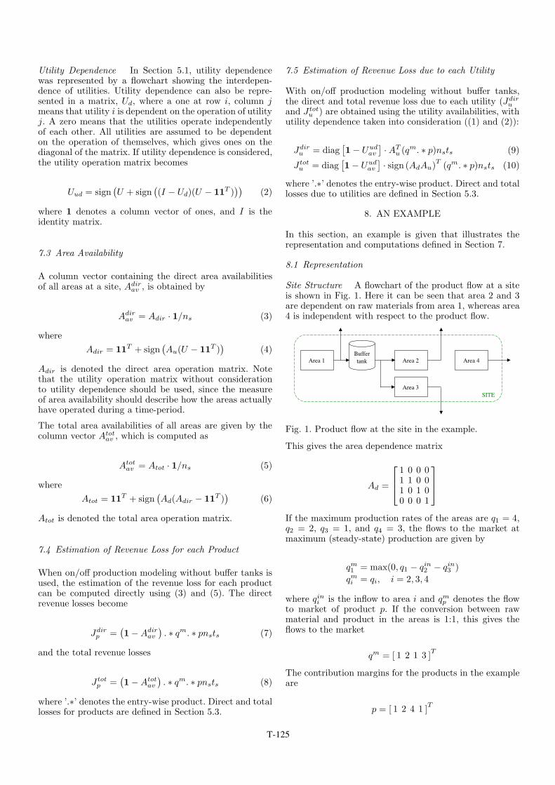
Site Structure A flowchart of the product flow at a siteis shown in Fig. 1. Here it can be seen that area 2 and 3are dependent on raw materials from area 1, whereas area4 is independent with respect to the product flow.

Fig. 1. Product flow at the site in the example.

This gives the area dependence matrix

Ad =

1 0 0 01 1 0 01 0 1 00 0 0 1

If the maximum production rates of the areas are q1 = 4,q2 = 2, q3 = 1, and q4 = 3, the flows to the market atmaximum (steady-state) production are given by

qm1 = max(0, q1 − qin2 − qin3 )qmi = qi, i = 2, 3, 4

where qini is the inflow to area i and qmp denotes the flowto market of product p. If the conversion between rawmaterial and product in the areas is 1:1, this gives theflows to the market

qm = [ 1 2 1 3 ]T

The contribution margins for the products in the exampleare

p = [ 1 2 4 1 ]T

T-125

Utility Measurement Data The example site requires thefive utilities: steam, cooling water, electricity, feed waterand instrument air. The corresponding utility parameters,that determine if the utility works correctly, are ’pressure’for steam, feed water and instrument air, and ’tempera-ture’ for cooling water. Electricity can only be operatingor not operating, i.e. ’on’ or ’off’. The measurements ofthe utility parameters during 10 hours with the samplinginterval 1 hour are given below

steam = [42 38 34 32 35 41 40 36 34 37]cooling water = [25 24 24 26 28 30 27 25 24 25]electricity = [1 1 1 1 1 1 0 1 1 1]feed water = [22 19 18 20 22 21 21 21 21 21]instrument air = [1 2 1 1 3 2 1 0 0 1]

The disturbance limits that have been set for these utilitiesat the site are:

Steam : pressure < 35 barCooling water : temperature > 27◦CElectricity : on/offFeed water : pressure < 20 barInstrument air : pressure ≤ 0 bar

which gives the utility operation matrix

U =

1 1 0 0 1 1 1 1 0 11 1 1 1 0 0 1 1 1 11 1 1 1 1 1 0 1 1 11 0 0 1 1 1 1 1 1 11 1 1 1 1 1 1 0 0 1

Utility Requirements Table 1 shows the utilities that arerequired by each area in this example.

Table 1. Utilities required at each area.

Area 1 Area 2 Area 3 Area 4

Steam x x

Cooling water x x

Electricity x x x x

Feed water x x

Instrument air x x x

This gives the area-utility matrix

Au =

1 0 1 1 10 1 1 0 01 1 1 1 10 0 1 0 1

8.2 Utility Availability

Using (1) we get the utility availabilities

Uav = U · 1/ns = [ 0.7 0.8 0.9 0.8 0.8 ]T

for the example site, if there are no planned stops in thedata set.

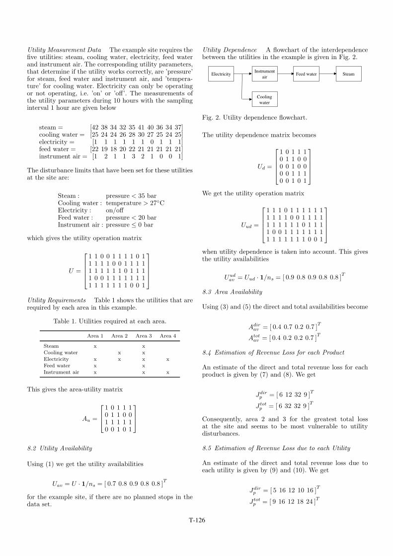
Utility Dependence A flowchart of the interdependencebetween the utilities in the example is given in Fig. 2.

Fig. 2. Utility dependence flowchart.

The utility dependence matrix becomes

Ud =

1 0 1 1 10 1 1 0 00 0 1 0 00 0 1 1 10 0 1 0 1

We get the utility operation matrix

Uud =

1 1 1 0 1 1 1 1 1 11 1 1 1 0 0 1 1 1 11 1 1 1 1 1 0 1 1 11 0 0 1 1 1 1 1 1 11 1 1 1 1 1 1 0 0 1

when utility dependence is taken into account. This givesthe utility availabilities

Uudav = Uud · 1/ns = [ 0.9 0.8 0.9 0.8 0.8 ]

T

8.3 Area Availability

Using (3) and (5) the direct and total availabilities become

Adirav = [ 0.4 0.7 0.2 0.7 ]

T

Atotav = [ 0.4 0.2 0.2 0.7 ]

T

8.4 Estimation of Revenue Loss for each Product

An estimate of the direct and total revenue loss for eachproduct is given by (7) and (8). We get

Jdirp = [ 6 12 32 9 ]

T

J totp = [ 6 32 32 9 ]

T

Consequently, area 2 and 3 for the greatest total lossat the site and seems to be most vulnerable to utilitydisturbances.

8.5 Estimation of Revenue Loss due to each Utility

An estimate of the direct and total revenue loss due toeach utility is given by (9) and (10). We get

Jdirp = [ 5 16 12 10 16 ]

T

J totp = [ 9 16 12 18 24 ]

T

T-126

This shows that instrument air causes the greatest totalloss at the site, which could be useful to know e.g. whendeciding where to focus maintenance efforts.

9. A TOOL FOR DISTURBANCE MANAGEMENT

A simple Matlab function for estimating the revenue lossesdue to utilities has been developed by the authors. Thistool can be used for any site by defining the equipmenthierarchy of the site, when the site and its utilities arerepresented by matrices, as described in Section 7. Theinputs to the function are the equipment hierarchy ofthe site, utility measurement data, the interdependenceof utilities, and the requirements of utilities in differentareas. The function returns utility and area availabilities,estimates of the revenue losses caused by each utility atthe site, and estimates of the loss corresponding to eachproduct due to utility disturbances. The estimates areobtained using on/off production modeling, as describedin this paper. In Matlab, the tool is run by

[Uav,Adirav,Atotav,Jdirp,Jtotp,Jdiru,Jtotu]=...= Tool_1(U,U_d,A_d,A_u,q_m,p)

using the notation from Section 7. This is a tool that maybe used for proactive disturbance management: The toolgives guidelines regarding for which utilities improvementefforts would be most profitable. An advantage with thistool is that it gives quick results with very little modelingeffort. A disadvantage is that it only gives relative results:ordering of utilities according to the revenue loss theycause. If also reactive disturbance management strategiesare desired, such as giving guidelines on how to reactto certain utility disturbances, a more advanced tool isrequired.

10. AN INDUSTRIAL EXAMPLE

The utility disturbance management tool has been usedfor the site at Perstorp studied in Lindholm et al. (2011a).This site has 10 areas and 14 utilities. Measurement datafrom August 1, 2007 to July 1, 2010 was used, with asampling interval of 1 minute. There was a planned stopbetween September 15 and October 8, 2009. This givesthe size (14 × 1501921) of the utility operation matrix.The estimates of the revenue losses for this example arecomputed by the Matlab script in less than one minute.

At the beginning of the case study, a survey was performedat the site, where operators where asked questions abouttheir perception of the frequency and severity of differentutility disturbances. The results from this survey seem toagree well with the results from the utility disturbancemanagement tool.

11. CONCLUSION

The suggested tool may be used to give decision supporton where proactive disturbance management efforts shouldbe focused at a site. The tool is easy to apply to anyprocess industrial site and can handle large sets of mea-surement data. The tool uses matrices that represent thesite structure, utility measurement data, interdependenceof utilities, and requirements of utilities at different areas.

ACKNOWLEDGEMENTS

The research is performed within the framework of theProcess Industrial Centre at Lund University, supportedby the Swedish Foundation for Strategic Research (SSF).

REFERENCES

Bansal, M., Adhitya, A., Srinivasan, R., and Karimi,I.A. (2005). An online decision support framework formanaging abnormal supply chain events. In proceedingsof the European Symposium on Computer Aided ProcessEngineering-15, 985–990.

Barroso, A.P., Machado, V.H., Barros, A.R., andMachado, V.C. (2010). Toward a resilient supply chainwith supply disturbances. In proceedings of the 2010IEEE International Conference on Industrial Engineer-ing and Engineering Management (IEEM), Macau, 245–249.

Brennan, D. (1998). Process Industry Economics: AnInternational Perspective. Institution of Chemical En-gineers.

ISA-95.00.01 (2009). Enterprise-Control System Integra-tion, Part 1: Models and Terminology. ISA.

ISO/WD-22400-2 (2011). Manufacturing operations man-agement - Key performance indicators - Part 2: Defini-tions and descriptions of KPIs. ISO. (draft).

Lindholm, A., Carlsson, H., and Johnsson, C. (2011a).Estimation of revenue loss due to disturbances on utili-ties in the process industry. In proceedings of the 22nd

Annual Conference of the Production and OperationsManagement Society (POMS), Reno, NV, USA.

Lindholm, A., Carlsson, H., and Johnsson, C. (2011b). Ageneral method for handling disturbances on utilities inthe process industry. In proceedings of the 18th WorldCongress of the International Federation of AutomaticControl (IFAC), Milano, Italy, 2761–2766.

Monostori, L., Szelke, E., and Kadar, B. (1998). Man-agement of changes and disturbances in manufacturingsystems. Annual Reviews in Control, (22), 85–97.

Niebert, P. and Yovine, S. (1999). Computing optimaloperation schemes for multi batch operation of chemicalplants. VHS deliverable. Draft.

T-127