Automatica 42 (2006) 1085–1093www.elsevier.com/locate/automatica

A Toeplitz algorithm for polynomial J-spectral factorization�

Juan Carlos Zúñigaa, Didier Henriona,b,∗aLAAS-CNRS, 7 Avenue du Colonel Roche, 31077 Toulouse, France

bDepartment of Control Engineering, Faculty of Electrical Engineering, Czech Technical University in Prague, Technická 2, 16627 Prague, Czech Republic

Received 29 September 2004; received in revised form 30 November 2005; accepted 20 February 2006Available online 17 April 2006

Abstract

A block Toeplitz algorithm is proposed to perform the J-spectral factorization of a para-Hermitian polynomial matrix. The input matrix canbe singular or indefinite, and it can have zeros along the imaginary axis. The key assumption is that the finite zeros of the input polynomialmatrix are given as input data. The algorithm is based on numerically reliable operations only, namely computation of the null-spaces of relatedblock Toeplitz matrices, polynomial matrix factor extraction and linear polynomial matrix equations solving.� 2006 Elsevier Ltd. All rights reserved.

Keywords: Polynomial matrices; Spectral factorization; Numerical algorithms; Computer-aided control system design

1. Introduction

1.1. Polynomial J-spectral factorization

In this paper we are interested in solving the following J-spectral factorization (JSF) problem for polynomial matrices:

Let A(s) = A0 + A1s + · · · + Adsd be an n-by-n polyno-mial matrix with real coefficients and degree d in the com-plex indeterminate s. Assume that A(s) is para-Hermitian, i.e.A(s)=AT(−s) where T denotes the transpose. We want to findan n-by-n polynomial matrix P(s) and a constant matrix J suchthat

A(s) = P T(−s)JP (s), J = diag{In+ , −In− , 0n0}. (1)

P(s) is non-singular and its spectrum1 lies within the left half-plane. J = J T is a signature matrix with +1, −1 and 0 alongthe diagonal, and such that n+ + n− + n0 = n.

� This paper was recommended for publication in revised form by Asso-ciate Editor Seip Weiland under the direction of Editor Roberto Tempo. Apreliminary version of this paper was presented at the IFAC Symposium onSystem, Structure and Control, Oaxaca, Mexico, December 8–10, 2004.

∗ Corresponding author. LAAS-CNRS, 7 Avenue du Colonel Roche, 31077Toulouse, France. Tel.: +33 561 33 63 08; fax: +33 561 33 69 69.

E-mail address: henrion@laas.fr (D. Henrion).1 The set of all the zeros (eigenvalues) of a polynomial matrix (Gohberg,

Lancaster, & Rodman, 1982b).

0005-1098/$ - see front matter � 2006 Elsevier Ltd. All rights reserved.doi:10.1016/j.automatica.2006.02.011

The J-spectral factorization of para-Hermitian polynomialmatrices has important applications in control and systems the-ory, as described first in Wiener (1949). See e.g. Kwakernaakand Šebek (1994) and Grimble and Kucera (1996) for com-prehensive descriptions of applications in multivariable Wienerfiltering, LQG control and H∞ optimization.

1.1.1. Factorization of singular matricesIn its most general form, the JSF problem applies to singu-

lar matrices. In this paragraph, we show that the problem offactorizing a singular matrix can be converted into the problemof factorizing a non-singular matrix. Alternatively, we can alsoseek a non-square spectral factor P(s).

If A(s) has rank r < n, then n+ + n− = r in the signaturematrix J. The null-space of A(s) is symmetric, namely if thecolumns of Z(s) form a basis of the right null-space of A(s), i.e.A(s)Z(s) = 0, then ZT(−s)A(s) = 0. As pointed out in Šebek(1990), the factorization of A(s) could start with the extractionof its null-space. There always exists an unimodular matrix

U−1(s) = [B(s) Z(s)]such that

U−T(−s)A(s)U−1(s) = diag{A(s), 0}, (2)

where the r × r matrix A(s) is non-singular. Now, if A(s) isfactorized as A(s) = P T(−s)J P (s), then the JSF of A(s) is

1086 J.C. Zúñiga, D. Henrion / Automatica 42 (2006) 1085–1093

given by

J = diag{J , 0}, P (s) = diag{P (s), In−r}U(s).

Equivalently, if we accept P(s) to be non-square, then we caneliminate the zero columns and rows in factorization (1) andobtain

A(s) = P T(−s)JP (s), J = diag{In+ , −In−}, (3)

where P(s) has size r × n. The different properties of factor-izations (1) and (3) are discussed later in Section 3.4.

What is important to notice here is that any singular factor-ization can be reduced to a non-singular one. Therefore, thetheory of non-singular factorizations can be naturally extendedto the singular case.

1.2. Existence conditions

Suppose that the full rank n-by-n matrix A(s) admits a fac-torization A(s)=P T(−s)JP (s) where constant matrix J T =J

has dimension m. Let �[A(s)] be the spectrum of A(s), then

m�m0 = maxz∈iR/�[A(s)]

V+[A(z)] + maxz∈iR/�[A(s)]

V−[A(z)],

where V+ and V− are, respectively, the number of positiveand negative eigenvalues of A(s) (Ran & Rodman, 1994).

If A(s) has no constant signature on the imaginary axis, i.e.the difference V+[A(z)] − V−[A(z)] is not constant for allz ∈ iR/�[A(z)], then n < m0 �2n, see the proof of Theorem3.1 in Ran and Rodman (1994).

On the other hand, if A(s) has constant signature, then m =m0 =n, and matrix J can be chosen as the unique square matrixgiven in (3). In Ran and Rodman (1994) it is shown that anypara-Hermitian matrix A(s) with constant signature admits aJSF. So, constant signature of A(s) is the basic existence con-dition for JSF that we will assume in this work.

In Ran and Zizler (1997) the authors give necessary and suf-ficient conditions for a self-adjoint polynomial matrix to haveconstant signature, see also Gohberg, Lancaster, and Rodman(1982a). These results can be extended to para-Hermitian poly-nomial matrices but this is out of the scope of this paper. Someother works giving necessary and sufficient conditions for theexistence of the JSF are Meinsma (1995) and Ran (2003).There, the conditions are related to the existence of an stabi-lizing solution of an associated Riccati equation. A deeper dis-cussion of all the related results on the literature would be veryextensive and also out of our objectives.

1.2.1. Canonical factorizationsIt is easy to see that if A(s) is para-Hermitian, then the

degrees �i for i = 1, 2, . . . , n of the n diagonal entries of A(s)

are even numbers. We define the diagonal leading matrix ofA(s) as

A = lim|s|→∞ =D−T(−s)A(s)D−1(s), (4)

where D(s) = diag{s�1/2, . . . , s�n/2}. We say that A(s) is di-agonally reduced if A exists and is non-singular. The JSF (3)

can be defined for both diagonally or non-diagonally reducedmatrices. From Kwakernaak and Šebek (1994) we say that theJSF of a diagonally reduced matrix A(s) is canonical if P(s) iscolumn reduced2 with column degrees equal to half the diag-onal degrees of A(s), see also Gohberg and Kaashoek (1986).

In this paper we extend the concept of canonical factorizationto matrices with no assumption on its diagonally reducedness(see Section 3.3) or even singular matrices (see Section 3.4).

1.3. Current algorithms and contributions

The interest in numerical algorithms for polynomial JSF hasincreased in the last years. Several different algorithms are nowavailable. As for many problems related to polynomial matrices,these algorithms can be classified in two major approaches: thestate-space approach and the polynomial approach.

The state-space methods usually relate the problem of JSFto the stabilizing solution of an algebraic Riccati equation. Oneof the first contributions was Tuel (1968), where an algorithmfor the standard sign-definite case (J = I ) is presented. Theevolution of this kind of methods is resumed in Stefanovski(2003) and references inside. This paper, based on the results ofTrentelman and Rapisarda (1999), describes and algorithm thatcan handle indefinite para-hermitian matrices (with constantsignature) with zeros along the imaginary axis. The case ofsingular matrices is tackled in Stefanovski (2004) only for thediscrete case.

The popularity of the state-space methods is related with itsgood numerical properties. There exist several numerical re-liable algorithms to solve the Riccati equation, see for exam-ple Bittanti, Laub, and Willems (1991). On the negative side,sometimes the reformulation of the polynomial problem interms of the state-space requires elaborated preliminary stepsKwakernaak and Šebek (1994) and some concepts and particu-larities of the polynomial problem are difficult to recover fromthe new representation. On the other hand, the advantage ofpolynomial methods is their conceptual simplicity and straight-forward application to the polynomial matrix, resulting, in gen-eral, in faster algorithms. On the negative side, the polynomialmethods are often related with elementary operations over thering of polynomials, and it is well known that these operationsare numerically unstable.

In this paper we follow the polynomial approach to develop anew numerically reliable algorithm for the most general case ofJSF. Our algorithm follows the idea of symmetric factor extrac-tion used first by Davis for the standard spectral factorization(Davis, 1963). Davis’ algorithm was improved in Callier (1985)and Kwakernaak and Šebek (1994) under the assumption thatthe polynomial matrix is not singular and has no zeros on theimaginary axis. Moreover, the computations are still based onunreliable elementary polynomial operations. Our contributions

2 Let q be the degree of the determinant of polynomial matrix P(s) andki the maximum degree of the entries of the ith column of P(s). Then P(s)

is column reduced if q = ∑ni=1 ki .

J.C. Zúñiga, D. Henrion / Automatica 42 (2006) 1085–1093 1087

are twofold:

(1) Generality: Our algorithm can handle the most generalcase of a possibly singular, indefinite para-Hermitian ma-trix, with no assumptions on its diagonally reducednessor the locations of its zeros along the imaginary axis. Asfar as we know, the only polynomial method which candeal with this general case is the diagonalization algorithmof Kwakernaak and Šebek (1994). The latter algorithm isbased on iterative elementary polynomial operations andthus, it can be quite sensitive to numerical round-off errors.

(2) Stability: No elementary polynomial operations are needed.Our algorithm is based on numerically reliable operationsonly, namely computation of the null-spaces of constantblock Toeplitz matrices along the lines sketched in Zúñigaand Henrion (2004a), factor extraction as described inHenrion and Šebek (2000), as well as solving linear poly-nomial matrix equations.

2. Eigenstructure and factor extraction

In this section we review some theory on polynomial matricesthat we use in our algorithm. Formal mathematics of this theorycan be found in the literature (Gohberg et al., 1982b). Here weadopt a practical approach and we present the results in a formconvenient for the sequel.

2.1. Eigenstructure of polynomial matrices

The eigenstructure of a polynomial matrix A(s) contains thefinite structure, the infinite structure and the null-space struc-ture.

2.1.1. Finite structureA finite zero of a non-singular polynomial matrix A(s) is a

complex number z such that there exists a non-zero complexvector v satisfying A(z)v = 0. Vector v is called characteristicvector or eigenvector associated to z.

If z is a finite zero of A(s) with algebraic multiplicity mA andgeometric multiplicity mG, then there exists a series of integerski > 0 for i=1, 2, . . . , mG such that mA=k1+k2+· · ·+kmG anda series of eigenvectors vi1, vi2, . . . , viki

for i = 1, 2, . . . , mGassociated to z such that⎡⎢⎢⎢⎢⎢⎣

A0 0

A1 A0

.... . .

Aki−1 · · · A1 A0

⎤⎥⎥⎥⎥⎥⎦

⎡⎢⎢⎢⎢⎢⎣

vi1

vi2

...

viki

⎤⎥⎥⎥⎥⎥⎦

= TZ[A(s), ki]V = 0 (5)

with v11, v21, . . . , vmG1 linearly independent and where

Aj = 1

j ![

djA(s)

dsj

]s=z

.

Integer ki is the length of the ith chain of eigenvectors associatedto z.

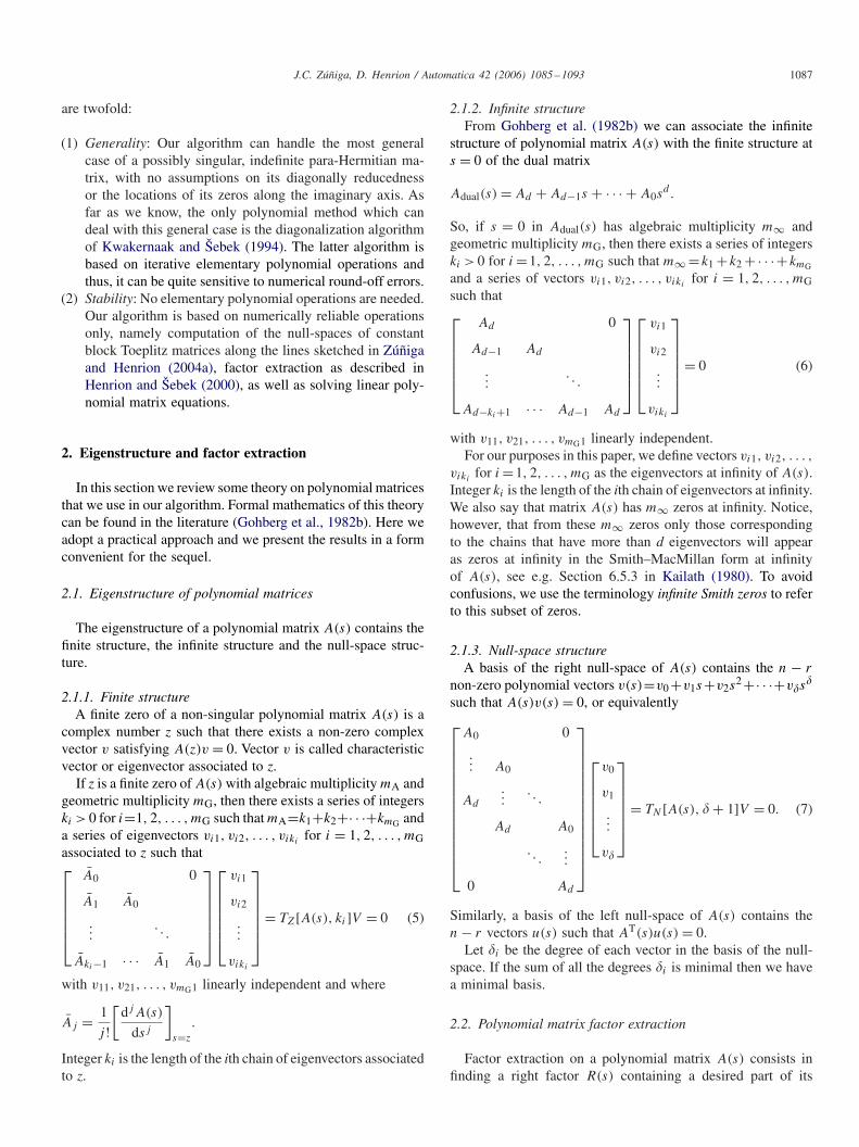
2.1.2. Infinite structureFrom Gohberg et al. (1982b) we can associate the infinite

structure of polynomial matrix A(s) with the finite structure ats = 0 of the dual matrix

Adual(s) = Ad + Ad−1s + · · · + A0sd .

So, if s = 0 in Adual(s) has algebraic multiplicity m∞ andgeometric multiplicity mG, then there exists a series of integerski > 0 for i =1, 2, . . . , mG such that m∞ =k1 +k2 +· · ·+kmG

and a series of vectors vi1, vi2, . . . , vikifor i = 1, 2, . . . , mG

such that⎡⎢⎢⎢⎢⎢⎣

Ad 0

Ad−1 Ad

.... . .

Ad−ki+1 · · · Ad−1 Ad

⎤⎥⎥⎥⎥⎥⎦

⎡⎢⎢⎢⎢⎢⎣

vi1

vi2

...

viki

⎤⎥⎥⎥⎥⎥⎦

= 0 (6)

with v11, v21, . . . , vmG1 linearly independent.For our purposes in this paper, we define vectors vi1, vi2, . . . ,

vikifor i =1, 2, . . . , mG as the eigenvectors at infinity of A(s).

Integer ki is the length of the ith chain of eigenvectors at infinity.We also say that matrix A(s) has m∞ zeros at infinity. Notice,however, that from these m∞ zeros only those correspondingto the chains that have more than d eigenvectors will appearas zeros at infinity in the Smith–MacMillan form at infinityof A(s), see e.g. Section 6.5.3 in Kailath (1980). To avoidconfusions, we use the terminology infinite Smith zeros to referto this subset of zeros.

2.1.3. Null-space structureA basis of the right null-space of A(s) contains the n − r

non-zero polynomial vectors v(s)=v0 +v1s+v2s2 +· · ·+v�s

�

such that A(s)v(s) = 0, or equivalently

⎡⎢⎢⎢⎢⎢⎢⎢⎢⎢⎢⎢⎢⎢⎣

A0 0

... A0

Ad

.... . .

Ad A0

. . ....

0 Ad

⎤⎥⎥⎥⎥⎥⎥⎥⎥⎥⎥⎥⎥⎥⎦

⎡⎢⎢⎢⎢⎢⎣

v0

v1

...

v�

⎤⎥⎥⎥⎥⎥⎦

= TN [A(s), � + 1]V = 0. (7)

Similarly, a basis of the left null-space of A(s) contains then − r vectors u(s) such that AT(s)u(s) = 0.

Let �i be the degree of each vector in the basis of the null-space. If the sum of all the degrees �i is minimal then we havea minimal basis.

2.2. Polynomial matrix factor extraction

Factor extraction on a polynomial matrix A(s) consists infinding a right factor R(s) containing a desired part of its

1088 J.C. Zúñiga, D. Henrion / Automatica 42 (2006) 1085–1093

eigenstructure, for instance a set of finite zeros with their re-spective chains of eigenvectors, and such that A(s)=L(s)R(s).Left factor L(s) contains the remainder of the eigenstructureof A(s). Nevertheless, it is not always possible to extract inR(s) any arbitrary part of the eigenstructure of A(s). Theoret-ical conditions are presented in Section 7.7 of Gohberg et al.(1982b). Here, in order to analyze this problem, and for theeffects of our algorithm, we use the following result extractedfrom Section 3.6 in Vardulakis (1991).

Lemma 1. The number of poles of a polynomial matrix A(s)

(it has only poles at infinity) is equal to the number k of finitezeros (including multiplicities) plus the number of infinite Smithzeros plus the sum dr of the degrees of the vectors in a minimalbasis of the right null-space of A(s) plus the sum dl of thedegrees of the vectors in a minimal basis of the left null-spaceof A(s) .

Corollary 2. Let A(s) be a polynomial matrix of degree d andrank r. Then

rd = k + m∞ + dr + dl.

Proof. Proof is direct from Lemma 1 and our definition ofzeros at infinity in Section 2.1.2.

Consider a square full-rank polynomial matrix A(s) of di-mension n and degree d with a set {z1, z2, . . . , zk} of finite ze-ros and with m∞ zeros at infinity. From Corollary 2 it followsthat nd = k + m∞. Suppose that we want to extract an n × n

factor R(s) of degree dR containing a subset of k finite zerosof A(s):

• If k = ndR and R(s) contains only the k finite zeros of A(s)

then we say that the factorization is exact.• If k is not an integer multiple of n, then the exact factorization

of a subset of k finite zeros of A(s) is not possible. In thiscase we can see that R(s) contains the k finite zeros but alsosome zeros at infinity.

The condition that the degree dR = k/n of factor R(s) shouldbe an integer is only a necessary condition to have an exactfactorization. We also require that equation L(s)R(s) = A(s)

can be solved for a polynomial factor L(s). Solvability of theabove polynomial matrix equation is related to the fact thatA(s) and the extracted factor R(s) have the same Jordan pairsassociated to the extracted zeros as explained in Chapter 7 ofGohberg et al. (1982b).

Example 3. Consider the matrix

A(s) =[

s −s2

1 0

]

which has two finite zeros at s = 0 and two zeros at infinity.Suppose that we want to extract exactly a factor R(s) contain-ing the two finite zeros. We can see that the degree of R(s)

should be dR = 2/2 = 1. For instance we can propose

R(s) =[

s 0

0 s

].

Nevertheless there is no solution L(s) for the polynomial equa-tion L(s)R(s) = A(s). As a result, R(s) is not a valid rightfactor of A(s). One possible factorization is given by

R(s) =[1 0

0 s2

], L(s) =

[s −1

1 0

].

Note that R(s) has the two finite zeros at s = 0 but also twozeros at infinity, so the factorization is not exact.

By analogy, we say that A(s) can have an exact factorizationof its infinite zeros whenever n∞ is an integer multiple of n.By duality, notice that zeros at the origin are introduced whenexact factorization is impossible, see Example 5.

When A(s) has rank r < n, from Corollary 2 we can see thatrd =k +m∞ +dl +dr where dl and dr. So, for A(s) to have anexact factorization of its right null-space, R(s) should have fullrow-rank equal to r and its degree dR should verify rdR = dr.When the factorization of the null-space is not exact, R(s) hasalso some zeros at infinity, see Examples 4 and 6.

3. The algorithm

As a basic assumption we consider that the finite zeros ofpolynomial matrix A(s) are given as input data. Finding thefinite zeros of a general polynomial matrix in a numerical soundway is a difficult problem in numerical linear algebra. The mostwidely accepted method consists in applying the QZ algorithmover a related pencil or linearization of A(s) (Moler & Stewart,1973). The QZ algorithm is backward stable, nevertheless itcan be shown that a small backward error in the coefficients ofthe pencil can sometimes yield large errors in the coefficientsof the polynomial matrix (Tisseur & Meerbergen, 2001). InLemonnier and Van Dooren (2004) an optimal scaling of thepencil is proposed and it is shown that the zeros of A(s) canbe computed with a small backward error in its coefficients.

Once the zeros of A(s) are given, we divide the problem ofJSF into two major parts: first the computation of the eigen-structure of A(s), second the extraction of factor P(s).

3.1. Computing the eigenstructure

In Zúñiga and Henrion (2004a) we outlined some blockToeplitz algorithms to obtain the eigenstructure of a polyno-mial matrix A(s). We showed how the infinite structure andthe null-space structure of A(s) can be obtained by solving it-eratively linear systems (6) and (7) of increasing size. We alsoshowed that if we know the finite zeros of A(s), then solvingiteratively systems (5) of increasing size allows to obtain thefinite structure.

In order to solve systems (5)–(7) we use reliable numericallinear algebra methods such as the singular value decomposition(SVD), the column Echelon form (CEF) or the LQ (dual to

J.C. Zúñiga, D. Henrion / Automatica 42 (2006) 1085–1093 1089

QR) factorization. All these methods are numerically stable,see for example Golub and Van Loan (1996). In Zúñiga andHenrion (2004b) we also presented a fast version of the LQfactorization and the CEF. The fast algorithms are based onthe displacement structure theory (Kailath & Sayed, 1999) andcan be a good option when the dimensions of systems (5)–(7)are very large. Numerical stability of fast algorithms is moredifficult to ensure however.

Preliminary results on the backward error analysis of the al-gorithms summarized in Zúñiga and Henrion (2004a) are pre-sented in Zúñiga and Henrion (2005). There we determine abound for the backward error produced by the LQ factoriza-tion in the coefficients of matrix A(s) when solving (5)–(7).We summarize here these results.

Consider that A(s) has a vector v(s) of degree � in the basisof its null-space. The computed vector v(s), obtained from (7)via the LQ factorization, is the exact null-space vector of theslightly perturbed matrix A(s)+�(s), where matrix coefficientsof perturbation polynomial matrix �(s)=�0+�1s+· · ·+�dsd

satisfy

‖�i‖2 �O(�)‖TN [A(s), � + 1]‖2.

where O(�) is a constant of the order of the machine precision �.Now consider that A(s) has a zero z and a chain of k as-

sociated eigenvectors {v1, v2, . . . , vk}. The computed vectors{v1, v2, . . . , vk} associated to the computed zero z, obtainedfrom (5) via the LQ factorization, are the exact vectors as-sociated to the exact zero z of the slightly perturbed matrixA(s) + �(s) with

‖�j‖2 �O(�)‖TZ[a(|z|), k]‖2,

and where a(s) = ‖Ad‖sd + · · · + ‖A0‖.

3.2. Extracting a polynomial factor

Consider a square non-singular n-by-n polynomial matrixA(s) with a set of finite zeros z = {z1, z2, . . . , zq}. The finitezero zj for j = 1, 2, . . . , q has a number mG of chains ofassociated eigenvectors, or geometric multiplicity. The ith chainof eigenvectors satisfies (5). For index i = 1, 2, . . . , mG definethe (d + 1)n-by-ki block Toeplitz matrix

Vi =

⎡⎢⎢⎢⎢⎢⎢⎢⎢⎣

vi1 vi2 · · · vi(ki−1) viki

vi0 vi1 · · · vi(ki−2) vi(ki−1)

vi(−1) vi0 · · · vi(ki−3) vi(ki−2)

...

vi(−d+1) vi(−d+2) · · · vi(−d+ki−1) vi(−d+ki )

⎤⎥⎥⎥⎥⎥⎥⎥⎥⎦

with vit =0 for t �0, and build up the matrix Wj =[V1 · · · VmG ]called the characteristic matrix of zj . Now suppose we wantto extract a factor R(s) containing the set of zeros z and suchthat A(s) = L(s)R(s). Since R(s) = R0 + R1s + · · · + Rdsd

contains the zero zj and shares the same eigenvectors,

equation (5) is also true for TZ[R(s), ki]. Note that this equationcan be rewritten as

[R0 R1 · · · Rd ]Vi = 0

and finally that

[R0 R1 · · · Rd ] = RS

= [R0 · · · Rd ]

⎡⎢⎢⎢⎢⎢⎣

I

zj I I

......

. . .

zdj I dzd−1

j I · · · I

⎤⎥⎥⎥⎥⎥⎦

.

So, since square matrix S is not singular, we can see that thecoefficients of R(s) can be obtained from a basis of the leftnull-space of a constant matrix, namely,

[R0 R1 · · · Rd ][W1 W2 · · · Wq ] = RW = 0.

To solve this last equation we can use some of the numeri-cal linear algebra methods mentioned above. Note that matrixW has a left null-space of dimension larger than n, in gen-eral. In other words, we have several options for the rows ofR(s). We choose the rows in order to have a minimum degreeand R(s) column reduced, for more details see Henrion andŠebek (2000). Column reducedness of factor R(s) controls theintroduction of infinite Smith zeros. As pointed out in Callier(1985), this control is important for the spectral symmetric fac-tor extraction. Nevertheless, notice that, even if R(s) has noinfinite Smith zeros, when the factorization is not exact it hassome zeros at infinity.

Example 4. Consider the matrix of Example 2. We want toextract a factor R(s) containing the two finite zeros at s = 0.With the algorithms of Zúñiga and Henrion (2004a) we obtainthe two characteristics vectors associated to s = 0

v1 =[0

1

], v2 =

[0

0

].

Then we can construct matrix

W =

such that a basis of its left null-space allows to find factor R(s):

[R0 R1 R2]W = W=0.

1090 J.C. Zúñiga, D. Henrion / Automatica 42 (2006) 1085–1093

Note that no pair of rows in the basis of the left null-space ofW gives a factor

R(s) =[

s 0

0 s

].

Choosing rows 1 and 4 we obtain a column reduced factor R(s)

which is the same as in Example 2.

Now we naturally extend these results to extract a factorsharing the same null-space as a square singular n × n poly-nomial matrix A(s) of rank r and degree d. Suppose that aminimal basis of the null-space of A(s) contains the vectorsvi(s) = vi0 + vi1s + · · · + vidi

sdi for i = 1, 2, . . . , n − r suchthat A(s)vi(s) = 0. Define the (d + 1)n-by-(di + d + 1) blockToeplitz matrix

Wi =

⎡⎢⎢⎣

vi0 · · · vidi0

. . .. . .

0 vi0 · · · vidi

⎤⎥⎥⎦ ,

and build up the matrix W = [W1 · · · Wn−r ]. Then we can seethat a factor R(s) = R0 + R1s + · · · + Rdsd sharing the samenull-space as A(s) can be obtained by solving the system

[R0 R1 · · · Rd ]W = 0.

Example 5. Consider the matrix

A(s) =⎡⎢⎣

s 0 1

s2 0 s

2s − s2 0 2 − s

⎤⎥⎦ .

We want to extract a factor R(s) sharing the same right null-space as A(s). With the algorithms of Zúñiga and Henrion(2004a) we obtain the vectors

v1(s) =⎡⎢⎣

0

1

0

⎤⎥⎦ , v2(s) =

⎡⎢⎣

−0.71

0

0.71s

⎤⎥⎦

generating a basis for the right null-space of A(s). Then wecan construct matrix

W =

⎡⎢⎢⎢⎢⎢⎢⎢⎢⎢⎢⎢⎢⎢⎢⎢⎢⎢⎢⎢⎣

0 0 0 −0.71 0 0 0

1 0 0 0 0 0 0

0 0 0 0 0.71 0 0

0 0 0 0 −0.71 0 0

0 1 0 0 0 0 0

0 0 0 0 0 0.71 0

0 0 0 0 0 −0.71 0

0 0 1 0 0 0 0

0 0 0 0 0 0 0.71

⎤⎥⎥⎥⎥⎥⎥⎥⎥⎥⎥⎥⎥⎥⎥⎥⎥⎥⎥⎥⎦

such that a basis of its left null-space allows to find factor R(s)

[R0 R1 R2]W = W = 0.

So, the minimum degree and rank r factor is

R(s) = [s 0 1].Note that R(s) has no zeros at infinity, so the factorization isexact.

Finally we sketch our algorithm for the JSF.

Algorithm spect. For an n × n para-Hermitian polynomialmatrix A(s) with constant signature, rank r and degree d, thisalgorithm computes the JSF A(s)=P T(−s)JP (s). We considerthat the set z of finite zeros of A(s) is given.

(1) If r < n, extract an r × n polynomial factor Rn(s) sharingthe same right null-space as A(s). Solve the polynomialequation

A(s) = RTn (−s)X1(s)Rn(s)

where X1(s) is a full-rank r×r polynomial matrix contain-ing only the finite zeros of A(s) and some zeros at infinity.If r = n let A(s) = X1(s).

(2) Extract a polynomial factor Rf(s) containing the finite lefthalf plane zeros of A(s) and half of its finite zeros on theimaginary axis. Solve the polynomial equation

X1(s) = RTf (−s)X2(s)Rf(s),

where X2(s) is a full-rank unimodular matrix.(3) Extract from X2(s) a factor R∞(s) containing half of its

zeros at infinity. Solve the polynomial equation

X2(s) = RT∞(−s)CR∞(s)

where C is a constant matrix such that CT = C.(4) Finally factorize C = UTJU . At the end we obtain the

searched spectral factor

P(s) = UR∞(s)Rf(s)Rn(s).

Reliable algorithms to solve polynomial equations of the typeA(s)X(s)B(s) = C(s) are based on iteratively solving linearsystems of equations, see documentation of functions axb, xaband axbc of the Polynomial Toolbox for Matlab (PolyX Ltd.,1998). Factorization of matrix C in step 4 is assured by theSchur algorithm (Golub & Van Loan, 1996).

3.3. Canonicity

When A(s) is positive definite, factorization in step 3 is al-ways exact and factor P(s) has always half of the zeros at in-finity of A(s), see Callier (1985). If A(s) is indefinite, there arecases where an exact factorization in step 3 is not possible. Forinstance consider that X2(s) results in the unimodular matrix of

J.C. Zúñiga, D. Henrion / Automatica 42 (2006) 1085–1093 1091

Example 3.3 in Kwakernaak and Šebek (1994). In that case notethat X2(s) can have a factorization with a non-minimal degreespectral factor.3 When A(s) is diagonally reduced, i.e. withoutSmith infinite zeros (Callier, 1985), this non-minimality in thefactorization of X2(s) implies that P(s) is not canonical in thesense of Kwakernaak and Šebek (1994). Nevertheless note that,even if we cannot conclude about the diagonal reducedness ofA(s), the non-minimality in the factorization of X2(s) can bedetected. So, in general we can say that a JSF is not canonicalif P(s) has more than half of the zeros at infinity of A(s).

Example 6. Consider the matrix

A(s) =[ 0 12 − 10s − 4s2 + 2s3

12 + 10s − 4s2 − 2s3 −16s2 + 4s4

]

which has finite zeros {−1, 1, −2, 2, −3, 3} and two zeros atinfinity. First we extract the factor

Rf(s) =[3 + 4s + s2 0

0 2 + s

]

containing the negative finite zeros of A(s), and we derive thefactorization

A(s) = RTf (−s)X2(s)Rf(s) = RT

f (−s)

[0 2

2 −4s2

]Rf(s).

Note that X2(s) is unimodular and has 4 zeros at infin-ity. The only column reduced factor containing 2 zerosat infinity that we can extract from X2(s) is given byR∞(s)=diag{1, s2}. Note that R∞(s) has also two finite zerosat 0, so the factorization is not exact. With Algorithm 3.2 ofKwakernaak and Šebek (1994)4 we can factorize X2(s) asX2(s) = RT∞(−s)diag{1, −1}R∞(s) with

R∞(s) =[1 1 − s2

1 −1 − s2

].

Finally, the spectral factor P(s) is given by

P(s) =[3 + 4s + s2 2 + s − 2s2 − s3

3 + 4s + s2 −2 − s − 2s2 − s3

].

Note that A given by (4) does not exist, we cannot concludeabout the diagonal reducedness of A(s), but we can say thatthe factorization is not canonical according to our definition.Spectral factor P(s) has finite zeros {−1, −2, −3} but also 3zeros at infinity, namely, more than half of the zeros at infinityof A(s).

3.4. Singular factorizations

When A(s) is rank deficient, we extract a non-square factorRn(s) at step 1. Equivalently we can extract a square factor as

3 In the sense that the degree of X2(s) is not the double of the degreeof R∞(s).

4 Numerical reliability of this algorithm is not guaranteed, however.

in (2) with the reliable methods presented in Henrion and Šebek(1999). Differences between both approaches are showed in thefollowing example.

Example 7. Consider the singular matrix

A(s) =⎡⎢⎣

s2 + s8 s + s7 s4

−s − s7 −1 − s6 −s3

s4 s3 1

⎤⎥⎦ .

Matrix A(s) has rank 2 and 14 zeros at infinity. A right null-space basis is given by v(s)=[−0.71 0.71s 0]T. A factor Rn(s)

sharing the same right null-space as A(s) is given by

Rn(s) =[0 0 1

s 1 0

],

so we have the factorization RTn (−s)X2(s)Rn(s) = A(s) with

X2(s) =[ 1 s3

−s3 −1 − s6

].

Matrix X2(s) has only zeros at infinity and it can be exactlyfactorized as X2(s) = RT∞(−s)diag{1, −1}R∞(s) with

R∞(s) =[1 s3

0 1

].

Therefore the non-square spectral factor P(s) is given by

P(s) = R∞(s)Rn(s) =[s4 s3 1

s 1 0

].

Note that A given by (4) has rank 1, we cannot concludeabout the diagonal reducedness of A(s), but we can say that thefactorization is canonical according to our definition. Spectralfactor P(s) has 7 zeros at infinity, namely, half of the zeros atinfinity of A(s). On the other hand, if at step 1 of the algorithmwe take a square factor Rn(s) such that RT

n (−s)X2(s)Rn(s) =A(s) with

X2(s) =⎡⎢⎣

−1 s3 0

−s3 1 + s6 0

0 0 0

⎤⎥⎦ ,

Rn(s) =⎡⎢⎣

s + s7 1 + s6 s3

s4 s3 1

1.4 + 0.71s6 0.71s5 0.71s2

⎤⎥⎦ ,

then square non-singular factor P(s) is given by

P(s) =⎡⎢⎣

s4 s3 1

s 1 0

1.4 + 0.71s6 0.71s5 0.71s2

⎤⎥⎦ .

In this case note that the factorization is not canonical accordingto our definition. Factor P(s) now has full rank, but this impliesthe introduction of zeros at infinity. P(s) has 18 zeros at infinity,namely, more than half of the zeros at infinity of A(s).

1092 J.C. Zúñiga, D. Henrion / Automatica 42 (2006) 1085–1093

4. Conclusions

A numerical algorithm for the polynomial matrix J-spectralfactorization was presented in this paper. In contrast with almostall the existing algorithms in the polynomial approach (Callier,1985; Kwakernaak & Šebek, 1994) our algorithm can deal witha possibly singular, indefinite polynomial para-Hermitian ma-trix with zeros along the imaginary axis. Moreover, no elemen-tary operations over polynomials are needed, and the algorithmis only based on numerically reliable operations:

• computation of the eigenstructure with the block Toeplitzmethods described in Zúñiga and Henrion (2004a);

• successive factor extractions along the lines described inHenrion and Šebek (2000);

• linear polynomial matrix equations solving.

Another approach to solving the J-spectral factorization prob-lem is the state-space approach, where the problem is relatedwith the solution of an algebraic Riccati equation. Maybe themost efficient algorithms with this approach are presented inStefanovski (2003) and Stefanovski (2004) for the discrete case.Our algorithm is as general as the algorithm in Stefanovski(2003) but we can also handle singular matrices using the null-space factor extraction presented here or the reliable triangu-larization methods of Henrion and Šebek (1999).

Direct comparisons between our algorithm and the algorithmin Stefanovski (2003) are difficult to achieve and it is out ofthe scope of this paper. We claim that both algorithms im-prove classical methods in their own style. On the one hand,algorithm in Stefanovski (2003) avoids some preparatory stepsusually necessary in the state-space approach via a minimalstate-space dimension. So, it brings improvements in terms ofcomputational effort. On the other hand, our algorithm avoidselementary operations over polynomials which are the basis ofstandard polynomial methods. So, it brings improvements interms of numerical stability.

Note, however, that global backward stability of algorithmspect cannot be guaranteed. Consider for example the null-space factor extraction: the null-space computed by algorithmsin Zúñiga and Henrion (2004a) is used as input of the factorextraction algorithm described here in Section 3.2. So, it is thesensitivity of the null-space structure problem that determineshow the backward error of the factor extraction algorithm isprojected into the coefficients of the analyzed polynomial ma-trix, and unfortunately this null-space problem is generally ill-posed.

Even if there exist satisfactory results on computing the fi-nite zeros of a polynomial matrix (Lemonnier & Van Dooren,2004), in practice, a real advantage of the state-space methodsover our algorithm is that they do not need to compute thesefinite zeros beforehand. Nevertheless notice that, by exploitingthe information on the eigenstructure of the polynomial matrix,further insight is lend into several cases of J-spectral factoriza-tion. Consider for example the non-canonical factorization: wehave seen that it is related with a non exact extraction of theinfinite structure of the polynomial matrix.

Another advantage of using the polynomial eigenstructure isthat our algorithm can be applied almost verbatim to the discretetime case.5 In fact, a discrete time polynomial matrix can beconsidered as a continuous time rational matrix. The structureat infinity of the discrete polynomial matrix is mapped into theinfinite structure and the structure at s = 0 of the associatedrational matrix. This fact explains the presence of the spuriouszeros Stefanovski (2004) but also allows us to handle themnaturally. For the discrete time case, factorization in step 3of the algorithm spect presented here, can be achieved intwo different ways: (1) by extracting a factor containing thefinite zeros at s = 0 (also zeros at infinity of the discrete timepolynomial matrix) and (2) by extracting a factor containingonly zeros at infinity. In the case (1) we recover the result ofAlgorithm 1 in Stefanovski (2004) with the presence of spuriouszeros, and in the case (2) we recover the result of Algorithm 2in Stefanovski (2004).

Acknowledgements

We are grateful to the reviewers and the associate editor forseveral constructive comments that significantly improved thepresentation of this work. We also would like to thank Paul VanDooren for insightful discussions on numerical stability issues.

Juan-Carlos Zúñiga acknowledges support from the NationalCouncil of Science and Technology of Mexico (CONACYT)as well as from the Secretariat of Public Education of Mexico(SEP). Didier Henrion acknowledges support from project No.102/05/0011 of the Grant Agency of the Czech Republic andproject No. ME 698/2003 of the Ministry of Education of theCzech Republic.

References

Bittanti, S., Laub, A. J., & Willems, J. C. (Eds.). (1991). The Riccati equation.Berlin: Springer.

Callier, F. M. (1985). On polynomial matrix spectral factorization bysymmetric extraction. IEEE Transactions on Automatic Control, 30(5),453–464.

Davis, M. C. (1963). Factoring the spectral matrix. IEEE Transactions onAutomatic Control, 8, 296–305.

Gohberg, I., & Kaashoek, M. A. (1986). Constructive methods of Wiener–Hopffactorization. Basel: Birkhäuser.

Gohberg, I., Lancaster, P., & Rodman, L. (1982a). Factorization of self-adjointmatrix polynomials with constant signature. Linear Multilinear Algebra,11, 209–224.

Gohberg, I., Lancaster, P., & Rodman, L. (1982b). Matrix polynomials. NewYork: Academic Press.

Golub, G. H., & Van Loan, C. F. (1996). Matrix computations. New York:The Johns Hopkins University Press.

Grimble, M., & Kucera, V. (Eds.). (1996). A polynomial approach to H2 andH∞ robust control design. London: Springer.

Henrion, D., & Šebek, M. (1999). Reliable numerical methods for polynomialmatrix triangularization. IEEE Transactions on Automatic Control, 44(3),497–508.

5 As pointed out in Stefanovski (2004) this is not possible with thestate-space methods.

J.C. Zúñiga, D. Henrion / Automatica 42 (2006) 1085–1093 1093

Henrion, D., & Šebek, M. (2000). An algorithm for polynomial matrix factorextraction. International Journal of Control, 73(8), 686–695.

Kailath, T. (1980). Linear systems. Englewood Cliffs, NJ: Prentice-Hall.Kailath, T., & Sayed, A. H. (1999). Fast reliable algorithms for matrices

with structure. Philadelphia: SIAM.Kwakernaak, H., & Šebek, M. (1994). Polynomial J-spectral factorization.

IEEE Transactions on Automatic Control, 39(2), 315–328.Lemonnier, D., & Van Dooren, P. (2004). Optimal scaling of block companion

pencils. International symposium on mathematical theory of networks andsystems. Belgium: Leuven.

Meinsma, G. (1995). J-spectral factorization and equalizing vectors. SystemsControl Letters, 25, 243–249.

Moler, C., & Stewart, G. W. (1973). An algorithm for generalized matrixeigenvalue problems. SIAM Journal on Numerical Analysis, 10, 241–256.

PolyX Ltd, (1998). The polynomial toolbox for matlab. Czech Republic:Prague, See www.polyx.com.

Ran, A. C. M. (2003). Necessary and sufficient conditions for existenceof J-spectral factorization for para-Hermitian rational matrix functions.Automatica, 39, 1935–1939.

Ran, A. C. M., & Rodman, L. (1994). Factorization of matrix polynomialswith symmetries. SIAM Journal on Matrix Analysis and Applications,15(3), 845–864.

Ran, A. C. M., & Zizler, P. (1997). On self-adjoint matrix polynomials withconstant signature. Linear Algebra Applications, 259, 133–153.

Šebek, M. (1990). An algorithm for spectral factorization of polynomialmatrices with any signature. Memorandum 912, Universiteit Twente, TheNetherlands.

Stefanovski, J. (2003). Polynomial J-spectral factorization in minimal state-space. Automatica, 39, 1893–1901.

Stefanovski, J. (2004). Discrete J-spectral factorization of possibly singularpolynomial matrices. System Control Letters, 53, 127–140.

Tisseur, F., & Meerbergen, K. (2001). The quadratic eigenvalue problem.SIAM Review, 43, 235–286.

Trentelman, H. L., & Rapisarda, P. (1999). New algorithms for polynomialJ-spectral factorization. Mathematics Control Signal Systems, 12, 24–61.

Tuel, W. G. (1968). Computer algorithm for spectral factorization of rationalmatrices. IBM Journal 163–170.

Vardulakis, A. I. G. (1991). Linear multivariable control. Algebraic analysisand synthesis methods. Chichester: Wiley.

Wiener, N. (1949). Extrapolation, interpolation and smoothing of stationarytime series. New York: Wiley.

Zúñiga, J. C., & Henrion, D. (2004a). Block Toeplitz Methods in PolynomialMatrix Computations. International symposium on mathematical theory ofnetworks and systems. Belgium: Leuven.

Zúñiga, J. C., & Henrion, D. (2004b). On the application of displacementstructure methods to obtain null-spaces of polynomial matrices. IEEEconference on decision and control, Paradise Island, Bahamas.

Zúñiga, J. C., & Henrion, D. (2005). Numerical stability of block Toeplitzalgorithms in polynomial matrix computations. IFAC world congress onautomatic control, Prague, Czech Republic.

Juan Carlos Zúñiga received the B.Sc. (Eng)degree in electrical engineering from the ITESOof Guadalajara, Mexico, in 1999. He obtainedthe M.Sc. degree from the CINVESTAV ofGuadalajara, Mexico, in 2001. From 2001 to2005 he made his Ph.D. thesis at the LAASof CNRS at Toulouse, France. He received thePh.D. degree from the INSA of Toulouse in2005. He is currently at the department of Math-ematics at the University of Guadalajara in Mex-ico. His research interests include Linear ControlSystems, Numerical Linear Algebra, NumericalPolynomial Algebra and Numerical algorithms.

Didier Henrion was born in Creutzwald,France, in 1971. He received the Masters’ andEngineer’s degrees from the National Institutefor Applied Sciences (INSA), Toulouse, France,in 1994, the Ph.D. degree from the Academyof Sciences of the Czech Republic, Prague,in 1998, and the Ph.D. degree from INSA in1999, all in the area of control. Since 2000 Di-dier Henrion has been a Researcher of CNRS(French National Center for Scientific Re-search) at LAAS (Laboratory of Analysis andArchitecture of Systems) in Toulouse. He also

holds a secondary appointment as a Researcher at the Faculty of Electri-cal Engineering of the Czech Technical University in Prague. His researchinterests are in numerical algorithms for polynomial matrices, convex op-timization over linear matrix inequalities, robust multivariable control, andcomputer-aided control system design. In 2004 he was awarded the BronzeMedal from CNRS. He is currently an associate editor of IFAC Automatica,European Journal of Control and IEEE Transactions on Automatic Control.