A time redundancy approach to TMR failures using fault ...

IEEE TRANSACTIONS ON COMPUTERS, VOL. 43, NO. 10, OCTOBER 1994 1151

A Time Redundancy Approach to TMR Failures Using Fault-State Likelihoods

Kang G. Shin, Fellow, IEEE, and Hagbae Kim, Member, IEEE

Abstract-Failure to establish a majority among the processing modules in a triple modular redundant (TMR) system, called a TMR failure, is detected by using two voters and a disagreement detector. Assuming that no more than one module becomes permanently faulty during the execution of a task, Re-execution of the task on the Same Hardware (RSHW) upon detection of a TMR failure becomes a cost-effective recovery method, because 1) the TMR s p e m can mask the effects of one faulty module while RSHW can recover from nonpermanent faults, and 2) system reconfiguration-Replace the faulty Hardware, reload, and Restart (RHWR)-is expensive both in time and hardware.

We propose an adaptive Wovery method for TMR failures by “optimally” choosing eithp RSHW or RHWR based on the estimation of the costs involved. We apply the Bayes theorem to update the likelihoods of all possible states in the TMR system with each voting result. Upon detection of a TMR failure, the expected cost of RSHW is derived with these likelihoods and then compared with that of RHWR. RSHW will continue either until it recovers from the TMR failure or until the expected cost of RSHW becomes larger than that of RHWR. As the number of unsuccessful RSHW’s increases, the probability of permanent fault@) having caused the TMR failure will increase, whicli will, in turn, increase the cost of RSHW. Our simulation results show that the proposed method outperforms the conventional reconfiguration method using only RHWR under various conditions.

Index Terms- Spatial and time redundancy, TMR failure, permanent and nonpermanent faults, reconfiguration, nominal task-execution time, likelihoods, Bayes theorem.

1. INTRODUCTION AULT tolerance is generally accomplished by using re- F dundancy in hardware, software, time, or combination

thereof. There are three basic types of redundancy in hardware and software: static, dynamic, and hybrid. Static redundancy masks faults by taking a majority of the results from replicated tasks [ 131. Dynamic redundancy takes a two-step procedure for detection of, and recovery from, faults [2]. The effectiveness of this method relies on selecting a suitable number of spares, a fault-detection scheme, and a switching operation. Hybrid redundancy is a combination of static and dynamic redundancy [4]. A core based on static hardware redundancy, and several spares are provided to tolerate faults. Such redundant systems

Manuscript received Ocober 15, 1992; revised May 10, 1993. This work reported was supported in part by the Office of Naval Research under Contract No. N00014-91-J-1115 and by the NASA under Grant No. NAG-1-1120. Any opinions, findings, and conclusions or recommendations expressed in this paper are those of the authors and do not necessarily reflect the view of the funding agencies.

The authors are with the Real-Time Computing Laboratory, Department of Electrical Engineering and Computer Science, The University of Michigan, Ann Arbor, MI 48109-2122 USA; e-mail: [email protected].

IEEE Log Number 9403024.

could provide very high reliability depending on the number of spares used under the assumption of perfect coverage and switching operation. However, new faults may occur during the detection of existing faults, and the switching operation becomes very complex as the number of spares increases. In order to reduce the complexity of switching operation and enhance reliability at low cost, self-purging [I21 and shift- out [5] schemes were developed, where faulty modules were removed but not replaced by standby spares. In these schemes, the additional operation required to select nonfaulty spare( s) is not needed, thus making the switching operation simpler. But it is difficult to implement either a threshold voter or a shift-out checking unit which requires comparators, detectors, and collectors.

Triple Modular Redundancy (TMR) has been one of the most popular fault-tolerance schemes using spatial redundancy. In the Fault-Tolerant MultiProcessor (FTMP) [6], com- putations are done on triplicated processors/memories connected by redundant common serial buses, and its quad- redundant clocks use bit-by-bit voting in hardware on all transactions over these buses. C.vmp [18] is also a TMR system which traded performance for reliability by switching between TMR mode with voting and independent modes under program control. In [22], an optimal TMR structure to recover from a transient fault was shown to extend significantly the lifetime of a small system in spite of its requirement of reliable voter circuits. The authors of [3] propdsed a modular TMR multiprocessor to increase reliability and availability by using a retry mechanism to recover transient faults, and switching between TMR and dual-processor modes to isolate a permanent fault. A simple multiple-retry policy (retry a pre-specified number of times)-also’ used to discriminate a permanent fault-was employed there. This policy can tolerate multiple faults only by treating them as a sequence of single faults with repair between fault occurrences, thus requiring freqbent voting for effective fault detection. A TMR failure caused by near-coincident faults in different modules must also be detected and recovered. The effect of dependent faults inducing a TMR failure wa? eliminated by periodic resynchronization at an optimal time interval [7]. However, the fault model of [7] and [22] did not include the possibility of permanent faults for which resynchronization is no longer effective.

In addition to the use of spatial redundancy with fault masking or reconfiguration, time redundancy can be applied effectively to recover from transient faults. Such recovery techniques are classified into instruction retry [lo], program

0018-9340/94$04.00 0 1994 IEEE

- ~~ ______ - _

mailto:[email protected]

1152 IEEE TRANSACTIONS ON COMPUTERS, VOL. 43, NO. 10, OCTOBER 1994

rollback [ 161, program reload and restart with module replacement. Several researchers attempted to develop an optimal recovery policy using time redundancy, mainly for simplex systems. Koren [9] analyzed instruction retries and program rollbacks with such design parameters as the number of retries and intercheckpoint intervals. Berg and Koren [2] proposed an optimal module switching policy by maximizing application- oriented availability with a pre-specified retry period. Lin and Shin [lo] derived the maximum allowable retry period by simultaneously classifying faults and minimizing the mean task-completion time.

The main intent of this paper is to develop an approach of combining time and spatial redundancy by applying time redundancy to TMR systems. (Note that spatial redundancy is already encapsulated in the TMR system.) When a TMR failure-failure to establish a majority due to multiple-module faults-is detected at the time of voting, or wherl a faulty module, even if its effects are masked, is identified, the TMR system is conventionally reconfigured to replace all three or just the faulty module with fault-free modules. If the TMR failure had been caused by transient faults, system reconfiguration or Replacement of Hardware and Restart (RHWR), upon detection of a TMR failure, may not be desirable due to its high cost in both time and hardware. To counter this problem, we propose to, upon detection of a TMR failure, Re-execute the corresponding task on the Same Hardware (RSHW) without module replacement. Instruction retry intrinsically assumes almost-perfect fault detection, for which TMR systems require frequent voting, thereby inducing high time overhead. However, the probability of system crash due to multiple-channel faults is shown in [17] to be insignificant for general TMR systems, even when $e outputs of computing modules are infrequently voted on as long as the system is free of latent faults. Unlike simplex systems, program rollback is not adequate for TMR systems due to the associated difficulty ctf checkpointing and synchronization. So, we consider re-execution of tasks on a TMR system with infrequent voting. For example, since more than 90% of faults are knawn p~ be nonpermanent-as few as 2% of field failures are caused by permanent faults [14]-simple re-execution may be an effective means to recover from most TMR failures. This may reduce 1) the hardware cost resulting from the hasty elimination of modules with transient faults and 2) the recovery time that would otherwise increase, Le., as a result of system reconfiguration. Note that system reconfiguration is time-consuming because it requires the location and replacement of faulty modules, program and data reloading, and resuming execution.

We shall propose two RSHW methods for determining when to reconfigure the system instead of re-executing a task without module replacement. The first (nonadaptive) method is to determine the maximum number of RSHW’s allowable (MNR) before reconfiguring the system for a given task according to its nominal execution time without estimating the system (fault) state-somewhat similar to the multiple-retry policy applied to a general rollback recovery scheme in [20]. By contrast, the second (adaptive) method 1) estimates the system state with the likelihoods of all possible states and 2) chooses

the better of RSHW or RHWR based on their expected costs when the system is in one of the estimated states. RHWR is invoked if either the number of unsuccessful RSHW’s exceeds the MNR in the first method or the expected cost of RSHW gets larger than that of RHWR in the second method. For the second method, we shall develop an algorithm for choosing between RSHW and RHWR upon detection of a TMR failure. We shall also show how to calculate the likelihoods of all possible states, and how to update them using the RSHW results and the Bayes theorem.

The paper is organized as follows. In the following section, we present a generic methodology of handling TMR failures, and introduce the assumptions used. Section I11 derives the optimal voting interval (X,) for a given nominal task-execution time X. The MNR of the first method and the optimal recovery strategy of the second method are computed for given X. We derive the probability density function (pdf) of time to the first occurrence of a TMR failure, the probabilities of all possible types of faults at that time, transition probabilities up to the voting time, the costs of RSHW and RHWR, and the problem of updating likelihoods of the system state and the recovery policy after an unsuccessful RSHW. Section IV presents numerical results and compares two recovery methods of RSHW and RHWR. The paper concludes with Section 5.

11. DETECTION AND RECOVERY OF A TMR FAILURE

Detection and location of, and the subsequent recovery from, faults are crucial to the correct operation of a TMR system, because the TMR system fails if either a voter fails at the time of voting or faults manifest themselves in multiple modules during the execution of a task. The fault occurrence rate is usually small enough to ignore coincident faults which are not caused by a common cause, but noncoincident fault arrivals at different modules are not negligible and may lead to a TMR failure.

Disagreement detectors which compare the values from the different voters of a TMR system can detect single faults, but may themselves become faulty. FTMP 161, JPL-STAR [l], and C.vmp [18] are example systems that use disagreement detectors. In FTMP, any detected disagreement is stored in error latches which compress fault-state information into error words for later identification of the faulty module(s). System reconfiguration to resolve the ambiguity in locating the source of a detected error is repeated depending on the source of the error and the number of units connected to a faulty bus. Two fault detection strategies-hard failure analysis (HFA) and transient failure analysis (TFA)-are provided according to the number and persistency of probable faulty units. These strategies may remove the unit(s) with hard failures or update the fault index (demerit) of a suspected unit. Frequent voting is required to make this scheme effective, because any faulty module must be detected and recovered before the occurrence of a next fault on another module within the same TMR system.

Voting in a TMR system masks the output of one faulty module, but does not locate the faulty module. One can, however, use a simple scheme to detect faulty modules and/or

1153 SHIN AND KIM: A TIME REDUNDANCY APPROACH TO TMR FAILURES USING FAULT-STATE LIKELIHOODS

processor 3

Fig. 1. The structure of a TMR system with two voters and a comparator.

voter. Assuming that the probability of two faulty modules producing an identical erroneous output is negligibly small, the output of a module-level voter becomes immaterial when multiple modules are faulty [8]. A TMR failure can then be detected by using two identical voters and a self-checking comparator as shown in Fig. 1. These voters can be imple- mented with conventional combinational logic design [ 2 3 ] . The comparator can be easily made self-checking. for its usually simple function: for example, a simple structure made of two-rail comparators in [l 13 for each bit can be utilized for its high reliability and functionality. q i s TMR structure can also detect a voter fault. When a TMR failure or a voter fault occurs, the comparator can detect the mismatch between the two voters that results from either the failure to form a majority among three processing modules, or a voter fault. (Note that using three voters, instead of two, would not make much difference in our discussion, so we will focus on a two-voter TMR structure.)

If the comparator indicates a mismatch between two voters at the time of voting, an appropriate recovery action must follow. Though RHWR has been widely used, RSHW may prove more cost-effective than RHWR in recovering from most TMR failures. To explore this in-depth, we will characterize RSHW with the way the MNR is determined. The simplest is to use a constant number of RSHW's irrespective of the nominal task-execution time and the system state which is defined by the number of faulty modules and the fault type(s). Taking into account the fact that the time overhead of an unsuccessful RSHW increases with the nominal task-execution time X, one can determine the MNR simply based on X, without estimating the system state. A more complex, but more effective, method is to decide between RSHW and RHWR based on the estimated system state. Since the system state changes dynamically, this decision is made by optimizing a certain criterion that is dynamically modified with the additional information obtained from each unsuccessful RSHW. In this adaptive method, the probabilities of all possible states will be used instead of one accurately-estimated state. Upon detection of a TMR failure, the expected cost of RSHW is updated and compared with that of RHWR. The failed task will then be re-executed, without replacing any module, either until RSHW recovers from the corresponding TMR failure or until the expected cost of RSHW becomes larger than that of task execution.' As the number of unsuccessful RSHW's

increases, the possibility of permanent faults having caused the TMR failure increases, which, in turn, increases the cost of RSHW significantly.

Throughout this paper, we assume that the arrival of permanent faults and the arrival and disappearance of nonpermanent faults are Poisson processes with rates A,, A,, and p, respectively.

111. O m A L RECOVERY FROM A TMR FAILURE USING RSHW

The Optimal Voting Interval

Let X, (2 5 z 5 n) be the nominal task-execution time measured in CPU cycles between the ( i - 1)th and ith voting, and let XI be that between the beginning of the task and the first voting, in the absence of any TMWvoter failure. As shown in Fig. 2, for 1 5 i 5 n let w, represent the task-execution time from the beginning of the task to the first completion of the zth voting possibly in the presence of some module failures, and let W, = E(w,). Then E(w,) = W, is the expected execution time of the task. Upon detection of a TMR failure, let p and q be tQp probabilities of recoverying a task with RSHW and RHW#, respectively, where p + q = 1. Assuming that the time overhead of reconfiguration is constant T,, W, is expressed as a recursive equation in terms of W,, 1 5 i 5 n. Let F,(t) (2 5 i 5 n) be the probability of a TMR failure in t units of time from the system state at the time of the ( j - 1)th voting, and let F l ( t ) be that from the beginning of the task. The probability of a recovery attempt (i.e., RSHW or RHWR) being successful depends upon F,(t). When a TMR failure is detected at the time of first voting (i.e., it occurred during the execution of the task portion corresponding to XI) , the system will try RSHW (or RHWR) with probability p (or q ) to recover from the failure. This process is renewed probabilistically for the variable w1 which is the actual task- execution time corresponding to the nominal task-execution time X1. Thus,

with probability 1 - Fl(X1) w 1 = X l + W l with probability F1 (X1)p

{X1 X1 + T, + w1 with probability Fl(X1)q

where T, is the setup time for system reconfiguration. Let Tu be the time overhead of voting that is in practice

negligible. The above equation is also renewed for all w,'s (2 5 i 5 n) after each successful recovery. Hence,

w, = w,-1 + V, + T,, for 2 5 a 5 n,

where V, is defined as the actual task-execution time between the (z - 1)th and zth votings, Le., VI = w1 and

with probability 1 - F,(X,) V , = X , + w , with probability F,(X,)p

{ X a X, + T, + w, with probability F,(X,)q.

From the above equations, the following recursive expressions are derived for 2 5 i 5 n:

' This procedure is described in the algorithm of Fig. 4.

1154

ep=* TMR failure

.-Tc-.- v, v, Y c-1: + E=27 0 : voting

W , Dl

Fig. 2. Graphical explanation for V, and w, for 1 5 z 5 n.

n 2 3 9 24 42 61

Applying thi? recursively n - 1 times, we can get:

The optimal voting frequency is derived by minimizing Wn with respect to n and Xi , 1 5 i 5 n, subject to

n

y x i = x . Y

i=l

If all inter-voting intervals are assumed to be identical then the constant voting interval is X i = X , = < for 1 5 i 5 n, where an optimal value of n must be determined by minimizing (3.1). Examples of n for a given X with typical values of p,q ,T , , and T, are shown in Table I. The voting points can be inserted by a programmer or a compiler.

Predetermination of Nonadaptive RSHW's

In the first method, we determine a priori the maximum number of RSHW's (MNR), k,, based on X without estimating the system spte. The associated task will be re-executed up to IC, times. As X increases, the effect of an unsuccessful RSHW becomes more pronounced; that is, the possibility of successful recovefy with RSHV (instead of RHWR) will decrease with X due to the increased rate of TMR failures, and the time overhead of an unsuccessful RSHW also increases with X while the time overhead of RHWR remains constant. So, IC, decreases as X increases.

Let C l ( k , X ) be the actual timekost of task execution in the presence of up to IC RSHW's for a task with the nominal execution time X, which can be expressed as:

k - 1

c1 ( k , X ) = xp; + 2 x p ; p : + . . . + kX J-J PZP! n=l

(3.2)

IEEE TRANSACTIONS ON COMPUTERS, VOL. 43, NO. 10, OCTOBER 1994

TABLE I1 k , vs. X FOR (P, F,R) = (0.8,0.1,0.8)

X / T , (hr.) 111 2ll 311 411 511

where p r ( p 2 ) and F l ( X ) denote the probability of the nth RSHW becoming successful (unsuccessful) and the probability of a TMR failure during X after system reconfiguration, respectively, where p: + p: = 1 , 1 5 n 5 k . In fact, p: and p: cannot be determined without knowledge of the system state after the (n - 1)th unsuccessful RSHW, which is too complicated to derive Q priori. We will approximate these probabilities using the following useful properties of a TMR system. Since the probability of permanent faults having caused the TMR failure increases with the number of unsuccessful RSHW's, p; is monotonically decreasing in n:

Though p i and R ( n ) p:+'/p: depend upon X and fault parameters, it is assumed for simplicity that p i is given a priori as a constant P and R(n) is a constant R for all n. Cl ( k , X ) of (3.2) is then modified in terms of P and R:

k-1 m-1

C l ( k , X ) = m X n ( 1 - P R n - l ) P R m - l m=l n=l

k-1

+ kX ( 1 - PRn-') n=l

+ ( Tc + ) f i (1 - PRn-1). (3.3) 1 - F 1 ( X ) n=l

The cost of RHWR, denoted by C z ( X ) , is derived by using recursive equations:

(3.4)

Now, k, can be determined as the iqteger that minimizes C l ( k , X ) subject to C l ( k , X > < C 2 ( X ) . Example values of IC, for typical values of P and R are shown in Table 11.

Adaptive RSHW

In this method, the system chooses, upon detection of a TMR failure, between RSHW and RHWR based on their expected costs. RSHW will continue either until it becomes successful or until the expected cost of the next RSHW becomes larger than that of RHWR. The system state is characterized by the likelihoods of all possible states because one can observe only the time of each TMR failure detection, which is insufficient to accurately estimate the system state. The outcome,of one RSHW, regardless whether it is successful or not, is used to update the likelihoods of states in one of which (called a prior state) the RSHW started. The possible states upon detection of a TMR failure can be inferred from the posterior states which are the updated prior states using the RSHW result and the Bayes theorem.

SHIN AND KIM: A TIME REDUNDANCY APPROACH TO TMR FAILURES USING FAULT-STATE LIKELIHOODS 1155

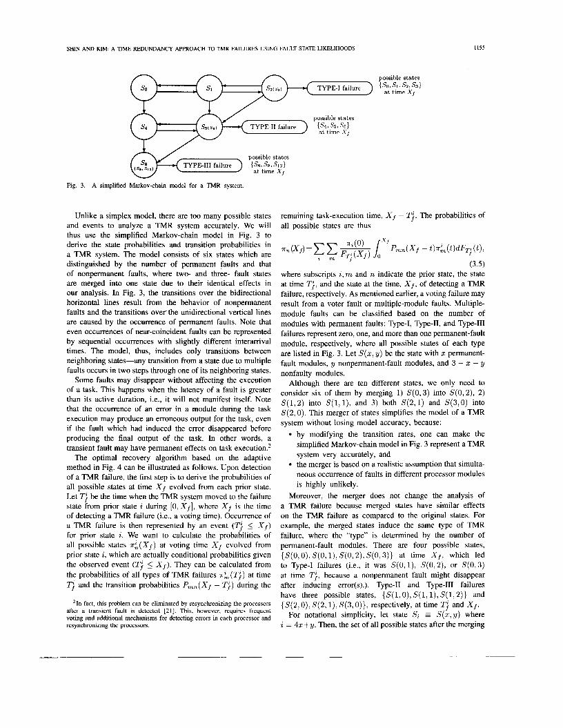
Fig. 3. A simplified Markov-chain model for a TMR system.

Unlike a simplex model, there are too many possible states and events to analyze a TMR system accurately. We will thus use the simplified Markov-chain model in Fig. 3 to derive the state probabilities and transition probabilities in a TMR system. The model consists of six states which are distinguished by the number of permanent faults and that of nonpermanent faults, where two- and three- fault states are merged into one state due to their identical effects in our analysis. In Fig. 3, the transitions over the bidirectional horizontal lines result from the behavior of nonpermanent faults and the transitions over' the unidirectional vertical lines are caused by the occurrence of permanent faults. Note that even occurrences of near-coincident faults can be represented by sequential occurrences with slightly different interarrival times. The model, thus, includes only transitions between neighboring states-any transition from a state due to multiple faults occurs in two steps through one of its neighboring states.

Some faults may disappear without affecting the execution of a task. This happens when the latency of a fault is greater than its active duration, i.e., it will not manifest itself. Note that the occurrence of an error in a module during the task execution may produce an erroneous output for the task, even if the fault which had induced the error disappeared before producing the final output of the task. In other words, a transient fault may have permanent effects on task execution.*

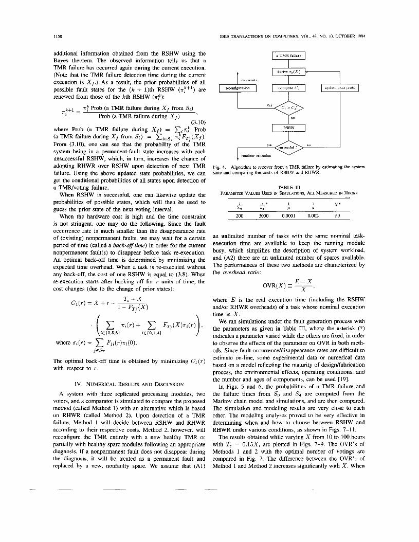
The optimal recovery algorithm based on the adaptive method in Fig. 4 can be illustrated as follows. Upon detection of a TMR failure, the first step is to derive the probabilities of all possible states at time X f evolved from each prior state. Let Tj be the time when the TMR system moved to the failure state from prior state i during [ O , X f ] , where X f is the time of detecting a TMR failure @e., a voting time). Occurrence of a TMR failure is then represented by an event (Ti < X f ) for prior state i. We want to calculate the probabilities of all possible states T ; ( X ~ ) at voting time X f evolved from prior state i, which are actually conditional probabilities given the observed event (Tj 5 X f ) . They can be calculated from the probabilities of all types of TMR failures 7ri(Tj) at time Tj and the transition probabilities Pm,(Xf - Tj ) during the

*In fact, this problem can be eliminated by resynchronizing the processors after a transient fault is detected [21]. This, however, requires frequent voting and additional mechanisms for detecting errors in each processor and resynchronizing the processors.

f. ..

remaining task-execution time, X f - Tj. The probabilities of all possible states are thus

where subscripts i, m and n indicate the prior state, the state at time Tj, and the state at the time, X f , of detecting a TMR failure, respectively. As mentioned earlier, a voting failure may result from a voter fault or multiple-module faults. Multiple- module faults can be classified based on the number of modules with permanent faults: Type-I, Type-11, and Type-I11 failures represent zero, one, and more than one permanent-fault module, respectively, where all possible states of each type are listed in Fig. 3. Let S(z, y) be the state with z permanent- fault modules, y nonpermanent-fault modules, and 3 - z - y nonfaulty modules.

Although there are ten different states, we only need to consider six of them by merging 1) S(O,3) into S(O,2), 2) S(1,2) into S(1, l), and 3) both S(2,l) and S(3,O) into S(2,O). This merger of states simplifies the model of a TMR system without losing model accuracy, because:

by modifying the transition rates, one can make the simplified Markov-chain model in Fig. 3 represent a TMR system very accurately, and the merger is based on a realistic assumption that simulta- neous occurrence of faults in different processor modules is highly unlikely.

Moreover, the merger does not change the analysis of a TMR failure because merged states have similar effects on the TMR failure as compared to the original states. For example, the merged states induce the same type of TMR failure, where the "type" is determined by the number of permanent-fault modules. There are four possible states, {S(O,O), S (0 , I), S(0 ,2) , S (0 ,3 ) ) at time X f , which led to Type-I failures (i.e., it was S(0 , l), S(0,2), or S(0 ,3) at time Tj, because a nonpermanent fault might disappear after inducing error(s).). Type-I1 and Type-I11 failures have three possible states, {S(l,O),S(l, l),S(l,2)} and {S (2 ,0 ) , S(2, l), S(3 ,0 ) ) , respectively, at time Tj and X f .

S(z,y) where i = 42+y. Then, the set of all possible states after the merging

For notational simplicity, let state S;


is {Si : i = 0,1 ,2 ,4 ,5 ,8}; out of these, {S1,Sp,S5,Sg} are the set of possible fault states transited from SO, SI, and S2 at time Tf", T j , and Tj , respectively. S4 and S5 may change to S5 (or s8) at T; (or T:), and S8 remains unchanged due to the persistence of a permanent fault.

Let a path denote the transition trajectory between a pair of states. Since there are usually more than one path between a given pair of nodes, each of these paths is assigned an ID number. From the simplified model in Fig. 3, Tj is the minimum-time path from Si to any type of TMR failure. Let t3 be the time taken from Si to a TMR failure via path j . Then,

the pdf s of all subpaths that make up path j . The pdf of a subpath between two states Sj, and Sjk+l is obtained by using the distribution of sojourn time t j , of Sj, with several exits in the Markov chain model (Fig. 3):

Ti - - minj [tj], where the pdf of ti is calculated by convolving

(3.6) where { E j , } represents the set of all outgoing arcs of Sj, . Then, the pdf of ti is

ft, ( t ) = fijl ( t ) * fjlj* ( t ) * . . . * f3," where path j is composed of subpaths {ijl,jlj2, . . . , j fm} and S, must be one of possible fault states: S,,, E {SI , SZ , S4 , SS , &}. (When the inter-arrival time of events such as fault occurrence, fault disappearance, and fault latency, is not exponentially distributed, we need a semi-Markov chain model in place of a Markov chain model.) Let J; represent the set of all paths to a fault state S, from Si. The likelihood of a fault state S, at time Tj is, then, equal to cjEJA F'rob(ti = Tj) , which is obtained by:

YEIE'I

where Ei is the set of all paths to all possible fault states

evolved from Si, i.e., Ei = u J k and m E {1,2,4,5,8} . The probabilities of S1 and S2 leading to Type-I failure are computed based on the behavior of nonpermanent faults, Le., depending on whether or not a nonpermanent fault, after having induced some error(s), is still active when a second nonpermanent fault occurs. Likewise, the probabilities of 5'4 and S5 leading to Type-I1 failure are computed by the behavior of a nonpermanent fault, if it had occurred earlier than permanent fault(s). When an intermittent fault is considered, the fault state must be divided by fault active and fault benign states as in [15], which makes the problem too complicated to be tractable. The numerical examples of FT;(X) and the mean of Tj (i = 0,4) for several X are given in Figs. 5 and 6, in which analytic results are compared against the results obtained from Monte-Carlo simulations.

m

In addition to fTE and T;, the transition probabilities P,, from S, to S: during X f - Tj must be derived in order to obtain the likelihood of every possible state at the time of voting (failure detection), X f . Although the matrix algebra using the transition matrix or Chapman-Kolmogrov theorem can be applied to give accurate expressions, we will use a simplified method for computational efficiency at an acceptably small loss of accuracy. For the transition probabilities from Tj, we need not consider subsequent errors but can focus on only those states useful in choosing between RSHW and RHWR.

Observe that the Occurrence rate, A,, of permanent faults is much smaller than both the appearance and disappearance rates of nonpermanent faults. Using this observation, one can analyze the behavior of permanent faults separately from that of nonpermanent faults. The transition probabilities due to the occurrence of permanent faults are represented by Pm,(Xj - Tj) for sm E { S ( ~ i , ~ ) ) , s , E {S(Z~,V) : xz > q}, that is, Pmn(Xf - Tj ) = 0 for S, E {S(zl,y)},S, E {S(Q, y) : $2 < XI}, because of the persistence of permanent faults. Although these probabilities depend upon 7rL(t) Vt, Tj 5 t 5 X f , they are approximated by using only the prior probabilities of source states, 7r& (Tj). This approximation causes only a very small deviation from the exact values because the Occurrence rate of permanent faults is usually very small as compared to the other rates. For example, consider Pl, for n 2 4, i.e., transitions from S1 due to the occurrence of permanent fault(s). The corresponding transition probabilities are derived from the model in Fig. 3 in terms of the pdf's of subpaths between two states. Let T = X f - Tj, then

T

pl8(T) = 1 F58(T - t)flS(t)dt

. l T ( 1 - F58(T - t))flS(t)dt.

The probability a:(Tj) for S1 is thus reduced to ( 1 - F15(T))~i (T")). Likewise, transitions from other source states due to the occurrence of permanent faults can be derived. Consequently, the prior probabilities are transformed into (1 -

respectively. Using these transformed prior probabilities, we will derive the transition probabilities based only on the behavior of nonpermanent faults.

Considering only the behavior of nonpermanent faults di- vides the above model into a two-state model (5'4, S5} and a three-state model {So, SI, S2}, as shown in Fig. 3. The transition matrix of the three-state model {SO, SI, Sa} is derived by 1) using the Laplace transform which reduces

F's (T)).; (Tj) i ( 1 - F48 (T))r i (Tj ) i and (1-F58 (T))rd (Tj ) 1


the linear differential equations of three states to algebraic equations in s, 2) solving the algebraic equations, and 3) transforming the solution back into the time domain.

The linear differential equation of {SO SI S2} with only the effects of nontransient faults is lI(Xf) = T ( X f - Tj)lI(Tj), where

2 q . -3Xn CL

T = b X n -2Xnp 2Xn -2p

The Laplace transform of T is:

s + 3Xn -/I 0

-2Xn s + 2 p A = [;3Xn s + 2Xnp - 2 p ] .

The solution requires the inverse of A (found at the bottom of the page).

Let the roots of s2 + (5Xn + 3p)s + 6Xg + 6 x 4 + 2p2 be a and p, then aij, the ijth element of A, can be obtained by partial fraction expansion:

C ( i j ) 2 C ( i j ) 3 +- s + a s + P '

C ( i j ) l I Q , . . - - 23 -

Since c(+ and c(ij)3 are conjugates, c(ij12 = k i j ( a l p) if c(ij)3 = kij(Pl a). The effect of permanent faults changes the initial probabilities of {Sol SI SZ): to:

n'(Tj) = [ A o ~ o ( T j ) , A i ~ i ( T j ) , A Z X Z ( ~ ' ~ ) ] ~ ~

where A0 = (1 - F O ~ ( T ) ) ~ A ~ = (1 - F I ~ ( T ) ) ~ A ~ = (1 - F25(T)). Thus, the ith column of the 3 x 3 transition matrix P(T) reduces to:

(3 + k3i(a1 p 1 e - a ~ + k3i(pl a)e-PT)Ai_l 1 1

($ + kli (a, p)e-aT + kli (pl a)e-PT)A;-l

(9 + k2i(al P)e-aT + k2i(pl a)e-PT)A;- l

x2 + (2Xn + 3p)x + 2p2 431 - x )

4 Y - x )

1 where

kll(X1Y) =

k22(x1 Y ) =

1

x2 + (3Xn + 2 p ) ~ + 6Xnp 1

x2 + (5Xn + P)X + 6 X i k33(xi Y ) =

X ( Y - x ) 1

The above equations indicate that the coefficients of exponen- tials in Ao, A I , and A2 include the effects of the occurrence of permanent fault(s) on the prior probabilities. Likewise, the transition matrix of a two-state model for (S4, Ss} can be derived from the matrix found at the bottom of the page where A4 = 1 - F48(T) and A5 = 1 - F58(T) also represent the effects of permanent-fault occurrences on the transitions to $3. These transition matrices and probabilities (resulting from the occurrence of permanent faults) can describe all possible transitions in the simplified model of Fig. 3.

When the TMR system is in S2, S5 or s8 at time Xf, RSHW will be unsuccessful again due to multiple active faults (in more than one module). If it is not in those states at time X f due to disappearance of active fault(s) after inducing some error(s), the system moves to a recoverable state by RSHW. Let FT;(X) be the probability of a TMR failure evolved from Si during the execution time X, where FTz is the probability distribution function of 7';. Since exact knowledge of the system state is not available, we estimate the state probabilities, which are then used to calculate the expected cost of a single RSHW as follows:

m . -7

where x ; ( O ) is the probability that the state before starting one RSHW (upon detecting a TMR failure) is Si, Le., the probabilities of the present states become those of the prior states for the next RSHW. The expected cost of RHWR is obtained similarly to (3.4):

m , ..jJ

(3.9)

When RSHW is unsuccessful or a voting failure occurs again, the (prior) state probabilities are updated with the


additional information obtained from the RSHW using the Bayes theorem. The observed information tells us that a TMR failure has occurred again during the current execution. (Note that the TMR failure detection time during the current execution is X f . ) As a result, the prior probabilities of all possible fault states for the (k + 1)th RSHW (T"') are renewed from those of the kth RSHW (T!):

= T: Prob (a TMR failure during X f from Si) z Prob (a TMR failure during X,) '

(3.10) where Prob (a TMR failure during X,) = xi.! Prob (a TMR failure during X f from Si) = xiEST afFT; ( X f ) . From (3.10), one can see that the probability of the TMR system being in a permanent-fault state increases with each unsuccessful RSHW, which, in turn, increases the chance of adopting RHWR over RSHW upon detection of next TMR failure. Using the above updated state probabilities, we can get the conditional probabilities of all states upon detection of a TMWvoting failure.

When RSHW is successful, one can likewise update the probabilities of possible states, which will then be used to guess the prior state of the next voting interval.

When the hardware cost is high and the time constraint is not stringent, one may do the following. Since the fault occurrence rate is much smaller than the disappearance rate of (existing) nonpermanent faults, we may wait for a certain period of time (called a back-ofStime) in order for the current nonpermanent fault( s) to disappear before task re-execution. An optimal back-off time is determined by minimizing the expected time overhead. When a task is re-executed without any back-off, the cost of one RSHW is equal to (3.8). When re-execution starts after backing off for T units of time, the cost changes (due to the change of prior states):

T, + X C l ( T ) = x + T +

- FTfo(x)

where .i(r) = Fji(r)ri(O). j E S T

The optimal back-off time is obtained by minimizing C ~ ( T ) with respect to T .

Iv . NUMERICAL RESULTS AND DISCUSSION

A system with three replicated processing modules, two voters, and a comparator is simulated to compare the proposed method (called Method 1) with an alternative which is based on RHWR (called Method 2). Upon detection of a TMR failure, Method 1 will decide between RSHW and RHWR according to their respective costs. Method 2, however, will reconfigure the TMR entirely with a new healthy TMR or partially with healthy spare modules following an appropriate diagnosis. If a nonpermanent fault does not disappear during the diagnosis, it will be treated as a permanent fault and replaced by a new, nonfaulty spare. We assume that (Al)

derive r , ( X )

re-execute

ly-?, FiSHW

-0.1 continue execution

Fig. 4. state and comparing the costs of RSHW and RHWR.

Algorithm to recover from a TMR failure by estimating the system

TABLE 111 PARAMETER VALUES USED IN SIMULATIONS, ALL MEASURED IN HOURS

200 3000 O.OOO1 0.002 50

an unlimited number of tasks with the same nominal task- execution time are available to keep the running module busy, which simplifies the description of system workload, and (A2) there are an unlimited number, of spares available. The performances of these two methods are characterized by the overhead ratio:

E - X OVR(X) - X '

where E is the real execution time (including the RSHW and/or RHWR overheads) of a task whose nominal execution time is X .

We ran simulations under the fault generation process with the parameters as given in Table 111, where the asterisk (*) indicates a parameter varied while the others are fixed, in order to observe the effects of the parameter on OVR in both methods. Since fault occurrence/disappearance rates are difficult to estimate on-line, some experimental data or numerical data based on a model reflecting the maturity of desigdfabrication process, the environmental effects, operating conditions, and the number and ages of components, can be used [19].

In Figs. 5 and 6, the probabilities of a TMR failure and the failure times from So and Sq are computed from the Markov-chain model and simulations, and are then compared. The simulation and modeling results are very close to each other. The modeling analyses proved to be very effective in determining when and how to choose between RSHW and RHWR under various conditions, as shown in Figs. 7-11.

The results obtained while varying X from 10 to 100 hours with T, = 0.15X, are plotted in Figs. 7-9. The OVR's of Methods 1 and 2 with the optimal number of votings are compared in Fig. 7. The difference between the OVR's of Method 1 and Method 2 increases significantly with X . When

SHIN AND KIM A TIME REDWANCY APPROACH TO TMR FAILURES USING FAULT-STATE LIKELIHOODS 1 I59

0.7

0.6

0.5 Prob.

(/Freq.) 0.4 of

TMR 0.3 failure

0.2

0.1

n

. ..e '

. "'1 P:SO - F:SO +- .' ' . '.O . . P:S4 - ~ 0'' '

F:S4 . o . - *'. . ( . . . e" '

10 2p 30 40 50 60 70 80 90 100

X: nominal computation [hour]

Fig. 5. ProbabilityFrequency of a TMR failure obtained from the Markov-chain model (PSO=from SO and P:S4=from S4)/from simulations (F:SO=from SO and F:S4=from S4).

60 -

50 - TMR 40 -

failure occurrence

t i m e 30 - 20 -

P:SO - F:SO - P:S4 ' 1 ' - F:S4 -

10 20 30 40 50 60 70 80 90 100


Fig. 6. Mean TMR failure time (E[Tfo]) obtained from analysis (P:SO=from So and PS4=from S4), and from simulations (F:SO=from SO and F:S4=from s4 ).

50 I I I I I I I I

45 - Method 1 +- Method 2

-

40 -

Overhead ratio

10 20 30 40 50 60 70 80 90 100

X: nominal comput,ation [hour]

Fig. 7. Overhead ratios [%] vs. X for RSHW and RHWR, with the optimal number of votings for Tu = 0.0005 hour: (13,34,61,87,110,133,164,181,198,216).

X is small, the OVR's of the two methods are too small to distinguish, which is due mainly to the small probability

60

50

40

Overhead 3o

20

10

0

ratio

multi +-

one e-

10 20 30 40 50 60 70 80 90 100

X : nominal computation [hour]

Fig. 8. optimal number of votings.

Overhead ratios [%] vs. X for one voting and multivotings with the

44 54 l Method Method 2 l -e- - A 14

Rat io 4

2 .5 3.i lT----7 1.5 t/

10 20 30 40 50 60 70 80 90 100


Ratio [%] of the number of reconfigurations to the total number of Fig. 9. simulation runs.

of a TMR failure. Fig. 8 compares the multivoting policy (with the optimal number of votings) and one voting policy. Generally, the overhead of a TMR system with infrequent voting increases significantly as X increases, because the probability of a TMR failure increases with X ; e.g., if there is no voting during the task execution, a TMR failure means the waste of the entire nominal execution time, X . As X increases, the OVR of a one-voting policy increases more rapidly than that of multivoting policy. The number of RHWR's-which is represented by the percentage of RHWR from the total number of simulations in Fig. 9-will determine the hardware cost of spares used. The increase in this percentage is much larger in Method 2 than Method 1, since the number of TMR failures increases with X , and Method 1 can recover from most TMR failures with RSHW.

The second comparison is made while varying !!',-the resetting time for system reconfiguration-from 2.5 to 12.5


Method 1 +- Method 2 -e-

11.5 -

Overhead rat io

lo t 1 9 . 5 +

2.5 5 7.5 10 12.5

Overhead rat io

Method 1 +- Method 2 -e- -

-

-

8 ‘ 1 I I I 5 10 15 20 25

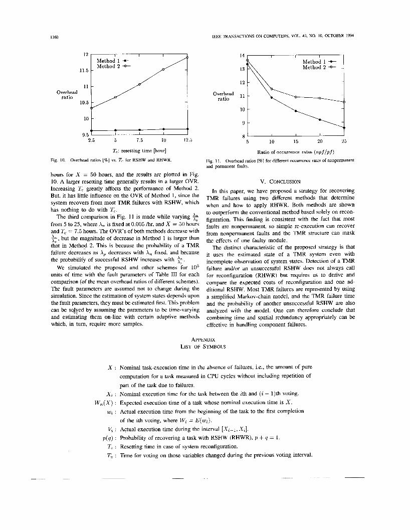
T,: resetting time [hour] Ratio of occurrence rates (npflpf) Fig. 10. Overhead ratios [%I vs. T, for RSHW and RHWR. Fig. 11,

and permanent faults. Overhead ratios [%I for different Occurrence rates of nonpermanent

hours for X = 50 hours, and the results are plotted in Fig. 10. A larger resetting time generally results in a larger OVR. V. CONCLUSION Increasing T, greatly affects the performance of Method 2. But, it has little influence on the OVR of Method 1, since the system recovers from most TMR failures with RSHW, which has nothing to do with T,.

The third comparison in Fig. 11 is made while varying 5 from 5 to 25, where A, is fixed at 0.005 /hr, and X = 50 hours and T, = 7.5 hours. The OVR’s of both methods decrease with

but the magnitude of decrease in Method 1 is larger than A, ’ that in Method 2. This is because the probability of a TMR failure decreases as A, decreases with A, fixed, and because the probability of successful RSHW increases with 5.

We simulated the proposed and other schemes for lo5 units of time with the fault parameters of Table I11 for each comparison (of the mean overhead ratios of different schemes). The fault parameters are assumed not to change during the simulation. Since the estimation of system states depends upon the fault parameters, they must be estimated first. This problem can be sqlyed by assuming the parameters to be time-varying and estimating them on-line with certain adaptive methods which, in turn, require more samples.

In this paper, we have proposed a strategy for recovering TMR failures using two different methods that determine when and how to apply RHWR. Both methods are shown to outperform the conventional method based solely on reconfiguration. This finding is consistent with the fact that most faults are nonpermanent, so simple re-execution can recover from nonpermanent faults and the TMR structure can mask the effects of one faulty module.

The distinct characteristic of the proposed strategy is that it uses the estimated state of a TMR system even with incomplete observation of system states. Detection of a TMR failure and/or an unsuccessful RSHW does not always call for reconfiguration (RHWR) but requires us to derive and compare the expected costs of reconfiguration and one additional RSHW. Most TMR failures are represented by using a simplified Markov-chain model, and the TMR failure time and the probability of another unsuccessful RSHW are also analyzed with the model. One can therefore conclude that combining time and spatial redundancy appropriately can be effective in handling component failures.

APPENDIX LIST OF SYMBOLS

X : Nominal task-execution time in the absence of failures, Le., the amount of pure computation for a task measured in CPU cycles without including repetition of part of the task due to failures.

X i : Nominal execution time for the task between the ith and (i - 1)th voting. W,(X) : Expected execution time of a task whose nominal execution time is X .

wi : Actual execution time from the beginning of the task to the first completion

V, : Actual execution time during the interval [Xi - l , X i ] . of the ith voting, where Wi = E(wi) .

p ( q ) : Probability of recovering a task with RSHW (RHWR), p + q = 1. T, : Resetting time in case of system reconfiguration. T, : Time for voting on those variables changed during the previous voting interval.


$($) : Probability of the nth RSHW being successful (unsuccessful). P : Probability of the first RSHW being successful.

R : Ratio of the probability of success at the (n + 1)th RSHW to that at the nth RSHW. IC, : Allowable maximum number of RSHW’s. X f : Time of detecting a TMWvoting failure. TJ : Time to a TMR system failure occurred first after starting the system in state S,.

FTt ( X ) : Probability of a TMR failure from S, during the execution time X (fT; pdf of TJ).

t: : Time of TMR failure occurrence via path J from Sa (f,. pdf of t;).

S(z, y) : State with z permanent faulty processor(s), y nonpermanent faulty processor(s), and (3 - z - y) nonfaulty processor(s) (S, = S(z, y) such that i = 42 + y).

m

Jh : Set of all paths to a fault state S, from an initial state Sa ( E z = u Jh). ~ ~ ( 0 ) : Probability of a prior state before the first RSHW.

T ~ ( T ; ) : Probability of a fault state S, at time T; from an initial state S,.

P,,(T) : Transition probability from S, to S, during T . Cl(lc, X ) : Expected cost of RSHW with a nominal task-execution time X and MNRA k

C l ( X ) ( C , ( X ) ) : Expected cost of RSHW (RHWR) for X . F3kJ(k+l) : Distribution of time to move to S3(k+l) from S J k .

{ E J k } : Set of all subpaths emanating from S J k . A,( A,) : Occurrence rate of nonpermanent (permanent) faults.

1 - : Active duration of a nonpermanent fault. P

ACKNOWLEDGMENT

The authors would like to thank A. White, C. Meissner, and F. Pitts of the NASA Langley Research Center, and J. Smith of the Office of Naval Research for their technical and financial assistance.

REFERENCES

[I ] A. Avizienis and G. C. Gilley, “The STAR (self-testing and repairing) computer: An investigation of theory and practice of fault-tolerant computer design,” IEEE Trans. Compur., vol. C-20, no. 11, pp. 1312-1321, Nov. 1971.

[2] M. Berg and I. Koren, “On switching policies for modular redundancy fault-tolerant computing systems,” IEEE Trans. Comput., vol. C-36, no. 9, pp. 1052-1062, Sept. 1987.

[3] P. K. Chande, A. K. Ramani, and P. C. Sharma, “Modular TMR multiprocessor system,” IEEE Trans. Indust. Electron., vol. 36, no. 1, pp. 3 U 1 , Feb. 1989.

[4] B. Cuchi, “Reliability and analysis of hybrid redundancy,” in Dig. Pap., FTCS-5, 1975, pp. 75-79.

[5] P. T. de Sousa and F. P. Mathur, “Shift-out modular redundancy,” IEEE Trans. Comput., vol. C-27, no. 7, pp. 624-627, July 1978.

[6] A. L. Hopkins, Jr., T. B. Smith, 111, and J. H. Lala, “FTMP-A highly reliable fault-tolerant multiprocessor for aircraft,” Proc. IEEE, vol. PROC-66, no. 10, pp. 1221-1239, Oct. 1978.

[7] M. Kameyama and T. Higuchi, “Design of dependent-failure-tolerant microcomputer system using triple-modular redundancy,” IEEE Trans. Comput., vol. C-29, no. 2, pp. 202-205, Feb. 1980.

[8] D. L. Kiskis and K. G. Shin, “Embedding triple-modular redundancy into a hypercube architecture,” in Proc. 3rd Conk HCCA, Los Angeles, CA, Jan. 1988, pp. 337-345.

[9] I. Koren and Z. Koren, “Analysis of a class of recovery procedures,” IEEE Trans. Comput., vol. C-35, no. 8, pp. 703-712, Aug. 1986.

[lo] T.-H. Lin and K. G. Shin, “An optimal retry policy based on fault classification,” IEEE Trans. Comput., vol. 43, no. 9, pp. 1014-1025, Sept. 1994.

[ 1 11 J.-C. Liu and K. G. Shin, “A RAM architecture for concurrent access and on-chip testing,” IEEE Trans. Comput., vol. 40, no. 10, pp. 1153-1 158, Oct. 1991.

[ 121 J. Losq, “A highly efficient redundancy scheme: Self-purging redundancy,’’ IEEE Trans. Comput., vol. C-25, no. 6, pp. 569-578, June 1976.

[ 131 R. E. Lyons and W. Vanderkulk, “The use of triple-modular redundancy to improve computer reliability,” IBM J. Res. Develop., vol. 6, pp. 2 W 2 0 9 , Apr. 1962.

[I41 S. R. McConnel, D. P. Siewiorek, and M. M. Tsao, “The measurement and analysis of transient errors in digital computer systems,” in Dig. Papers, FTCS-9, June 1979, pp. 67-70.

[I51 K. G. Shin and Y.-H. Lee, “Error detection process-Model, design, and its impact on computer performance,’’ IEEE Trans. Comput., vol. C-33, no. 6, pp. 529-539, June 1984.

[I61 K. G. Shin, T.-H. Lin, and Y.-H. Lee, “Optimal checkpointing of real- time tasks,” IEEE Trans. Comput., vol. C-36, no. 11, pp. 1328-1341, Nov. 1987.

[ 171 K. G. Shin and J.-C. Liu, “Study on fault-tolerant processor for advanced launch system,” NASA Contractor Rep., June 1990.

[I81 D. P. Siewiorek, V. Kini, and H. Mashbum, “A case study of Cmmp, Cm*, and C.vmp: Part I-Experiences with fault tolerance in multiprocessor systems,” Proc. IEEE, vol. PROC-66, no. 10, pp. 1178-1 199, Oct. 1978.

[19] D. P. Siewiorek and R. S. Swarz, The Theory and Practice of Reliable System Design.

[20] J. S. Upadhyaya and K. K. Saluja, “A watchdog processor based general rollback technique with multiple retries,” IEEE Trans. Soffware Eng., vol. SE-12, no. 1, pp. 87-95, Jan.. 1986.

[21] J. F. Wakerly, “Transient failures in triple modular redundancy systems with sequential modules,” IEEE Trans. Compur., vol. 33, no. 5 , pp. 57C573, May 1975.

[22] - , “Microcomputer reliability improvement using triple-modular redundancy,” IEEE Trans. Comput., vol. 34, no. 6, pp. 889-895, June 1976.

[23] X.-Y. Zhuo and S.-L. Li, “A new design method of voter in fault- tolerant redundancy multiple-module multi-microcomputer system,” in Dig. Pap., FTCS-13, June 1983, pp. 472475.

Bedford, MA: Digital Equipment Corporation, 1982.

1162

Kang G. Shin (S’75-M’78-SM’83-F‘92) received the B.S. degree in electronics engineering from Seoul National University, Seoul, Korea in 1970, and both the M.S. and Ph.D. degrees in electrical engineering from Comell University, Ithaca, New York in 1976 and 1978, respectively.

He is a Professor of Electrical Engineering and Computer Science for the Computer Science and Engineering Division, The University of Michigan, Ann Arbor, MI. He also chaired the CSE Divi- sion for three years beginnine 1991. From 1978 to

1982 he was on the faculty of Rensselaer Polytechnic Institute, Troy, New York. He has held visiting positions at the U.S. Airforce Flight Dynamics Laboratory, AT&T Bell Laboratories, Computer Science Division within the Department of Electrical Engineering and Computer Science at UC Berkeley, and International Computer Science Institute, Berkeley, CA. He has also been applying the basic research results of real-time computing to manufacturing-related applications ranging from the control of robots and machine tools to the development of open architectures for manufacturing equipment and processes. Recently, he has initiated research on the open- architecture Information Base for machine tool controllers.

Dr. Shin has authoredcoauthored over 270 technical papers (about 130 of these in archival joumals) and several book chapters in the area of distributed real-time computing and control, fault-tolerant computing, computer architecture, robotics and automation, and intelligent manufacturing. In 1987, he received the Outstanding IEEE Transactions on Automatic Control Paper Award for a paper on robot trajectory planning. In 1989, he also received the Research Excellence Award from The University of Michigan. In 1985, he founded the Real-Time Computing Laboratory, where he and his colleagues are currently building a 19-node hexagonal mesh multicomputer, called HARTS, to validate various architectures and analytic results in the area of distributed real-time computing. He was the Program Chairman of the 1986 IEEE Real-Time Systems Symposium (RTSS), the General Chairman of the 1987 RTSS, the Guest Editor of the 1987 August special issue of IEEE TRANSACTIONS ON COMPUTERS on Real-Time Systems, a Program Co-Chair for the 1992 Intemational Conference on Parallel Processing, and served numerous technical program committees. He also chaired the IEEE Technical Committee on Real-Time Systems during 1991-93, is a Distinguished Visitor of the Computer Society of the IEEE, an Editor of IEEE TRANSACTIONS ON PARALLEL AND DISTRIBUTED COMPUTING, and an Area Editor on Intemational Joumal of Time-Critical Computing Systems.

IEEE TRANSACTION

8

S ON COMPUTERS, VOL. 43, NO. 10, OCTOBER 1994

Hagbae Kim (S’90-M’94) received the B.S. degree from in electronics engineering frofn Seoul National University, Seoul, Korea, in 1988, and the M.S. and Ph.D. degrees in electrical engineering from the University of Michigan, Ann Arbor, in 1990 and 1994, respectively

Currently, he is a Research Associate at NASA Langley Research Center, Hampton, VA. His current research interests include real-time control systems, fault-tolerant computing, reliability modeling, and probability and stochastic processes.

A time redundancy approach to TMR failures using fault ...

Documents

Transcript of A time redundancy approach to TMR failures using fault ...