Salient pole rotor vs. non salient pole rotor electricaleasy
A Three-pathway Psychobiological Framework of Salient Object Detection
Using Stereoscopic Technology
Chunbiao Zhu
SECE, Shenzhen Graduate School
Peking University
Shenzhen, China
Ge Li∗
SECE, Shenzhen Graduate School
Peking University
Shenzhen, China∗
Abstract
Saliency detection, finding the most important parts of
an image, has become increasingly popular in computer vi-
sion. Existing proposal methods are mostly based on color
information, which may not be effective for cluttered back-
grounds. We propose a new algorithm leveraging stereop-
sis to generate optical flow which can obtain addition cue
(depth cue) to get the final saliency map. The proposed
framework consists of three pathways. The first pathway
eliminates the background based on cellular automata. The
second pathway gets the optical flow and color flow saliency
map. The third pathway calculates a coarse saliency map.
Finally, we fuse these three pathways to generate the final
saliency map. Besides, we construct a new high-quality
dataset with the complex scene to make computer challenge
human vision. Experimental results on our dataset and an-
other three popular datasets demonstrate that our method
is superior to the existing methods in terms of robustness.
1. Introduction
Saliency detection is a process of getting the visual at-
tention region precisely. The attention is the behavioral and
cognitive process of selectively concentrating on one aspect
of the environment while ignoring other things, which re-
sponses how we actively process specific information in our
environment.
Early works on computing saliency aim to locate the
visual attention region. Recently the field has been ex-
tended to locate and refine the salient regions and objects.
Served as a fundamental of various multimedia applica-
tions [2, 5, 5, 15], salient object detection is widely used in
content-aware editing, image retrieval, object recognition,
object segmentation, compression, image retargeting, etc.
In general, saliency detection algorithms mainly use top
down or bottom-up approaches. Top-down approaches are
task-driven and need supervised learning. While bottom-up
approaches usually use low-level cues, such as color fea-
tures, distance features and other heuristic saliency features.
The most used features are heuristic saliency features and
discriminative saliency features. Various measures based
on heuristic saliency features have been proposed, includ-
ing pixel-based or patch-based contrast, region-based con-
trast, pseudo-background, and similar images. Notwith-
standing the demonstrated success, existing RGB-based al-
gorithms [9, 16] may become ineffective when objects can-
not be easily separated from the background (e.g., objects
with similar colors to the background). In this case, addi-
tional cues are required as a complement to detect the ob-
jects from the image.
Recently, advances in the rapid deployment of stereo-
scopic equipment have motivated the adoption of structural
features, improving discrimination among different objects
with the similar appearance. As a complement to color im-
ages, a stereo image pair is utilized to obtain rough depth
and edge correspondences for the two images. Some algo-
rithms [3, 6, 4, 14, 1] adopt depth cue which is generated
by stereo image pairs to deal with the complex scenarios.
In [3], Cheng et al. compute salient stimuli in both color
and depth spaces. In [6], Ju et al. propose a saliency method
that works on depth images based on the anisotropic center-
surround difference. In [4], Guo et al. propose a salient
object detection method for RGB-D images based on evo-
lution strategy. Their results show that stereo saliency is a
useful consideration compared to previous visual saliency
analysis. In [1], an active vision system is presented for vi-
sual scene segmentation based on the integration of several
cues. These methods combine a set of foveal and periph-
eral cameras. Object hypotheses are generated through a
stereo based fixation process. In [14], depth cues are used
to enhance the salient object detection results. All of them
demonstrate the effectivity of depth cue in the improvement
of salient object detection.
3008
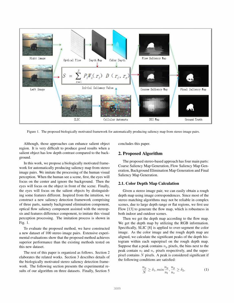
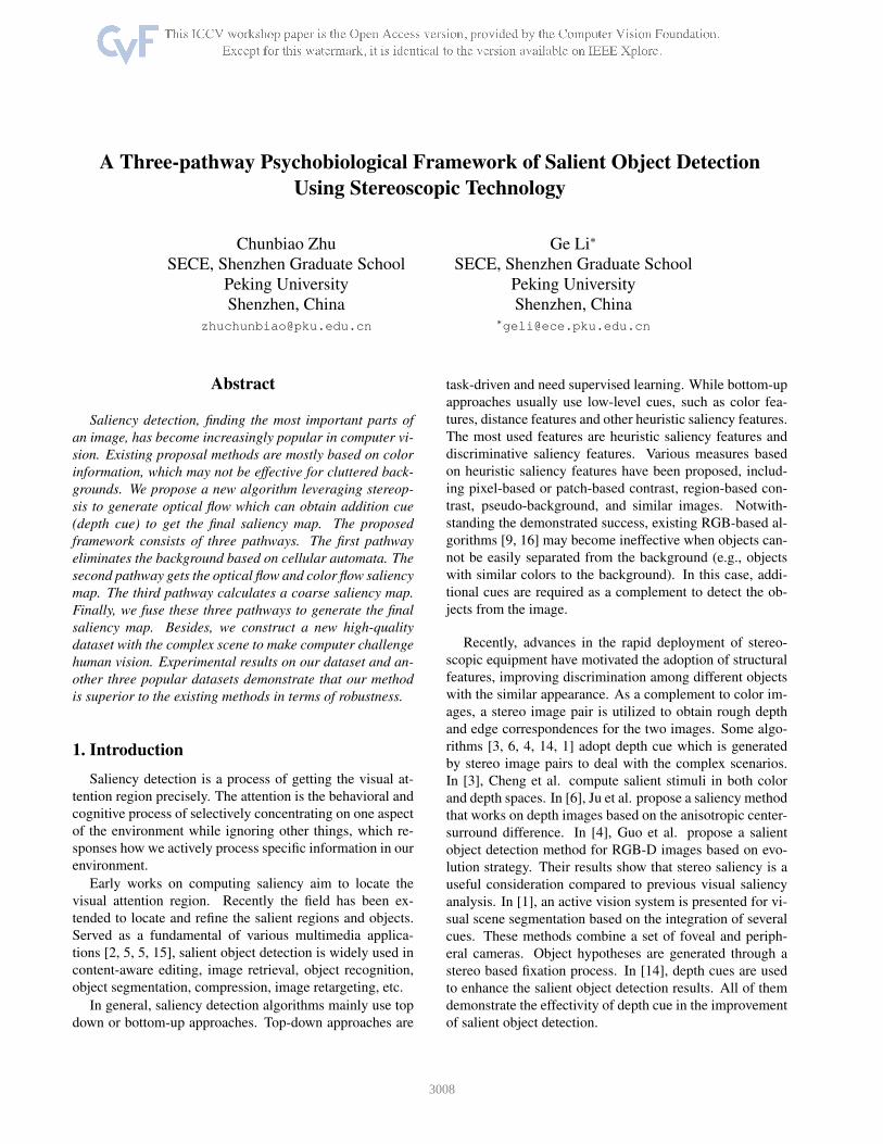
Figure 1. The proposed biologically motivated framework for automatically producing saliency map from stereo image pairs.
Although, those approaches can enhance salient object
region. It is very difficult to produce good results when a
salient object has low depth contrast compared to the back-
ground.
In this work, we propose a biologically motivated frame-
work for automatically producing saliency map from stereo
image pairs. We imitate the processing of the human visual
perception. When the human see a scene, first, the eyes will
focus on the center and ignore the background. Then the
eyes will focus on the object in front of the scene. Finally,
the eyes will focus on the salient objects by distinguish-
ing some features different. Inspired from the intuition, we
construct a new saliency detection framework comprising
of three parts, namely background elimination component,
optical flow saliency component assisted with the stereop-
sis and features difference component, to imitate this visual
perception processing. The imitation process is shown in
Fig. 1.
To evaluate the proposed method, we have constructed
a new dataset of 100 stereo image pairs. Extensive experi-
mental evaluations show that the proposed method achieves
superior performance than the existing methods tested on
this new dataset.
The rest of this paper is organized as follows. Section 2
elaborates the related works. Section 3 describes details of
the biologically motivated stereo saliency detection frame-
work. The following section presents the experimental re-
sults of our algorithm on three datasets. Finally, Section 5
concludes this paper.
2. Proposed Algorithm
The proposed stereo-based approach has four main parts:
Coarse Saliency Map Generation, Flow Saliency Map Gen-
eration, Background Elimination Map Generation and Final
Saliency Map Generation.
2.1. Color Depth Map Calculation
Given a stereo image pair, we can easily obtain a rough
depth map using image correspondences. Since most of the
stereo matching algorithms may not be reliable in complex
scenes, due to large depth range or flat regions, we first use
Flow [13] to generate the flow map, which is robustness in
both indoor and outdoor scenes.
Then we get the depth map according to the flow map.
We get the depth map by utilizing the RGB information.
Specifically, SLIC [8] is applied to over-segment the color
image. As the color image and the rough depth map are
aligned, we calculate the significant peaks of the depth his-
togram within each superpixel on the rough depth map.
Suppose that a peak contains np pixels, the bins next to the
peak contain nl and nr pixels respectively, and the super-
pixel contains N pixels. A peak is considered significant if
the following conditions are satisfied:
np
N≥ δ1,min
np
nl
,np
nr
≥ δ2, (1)
3009
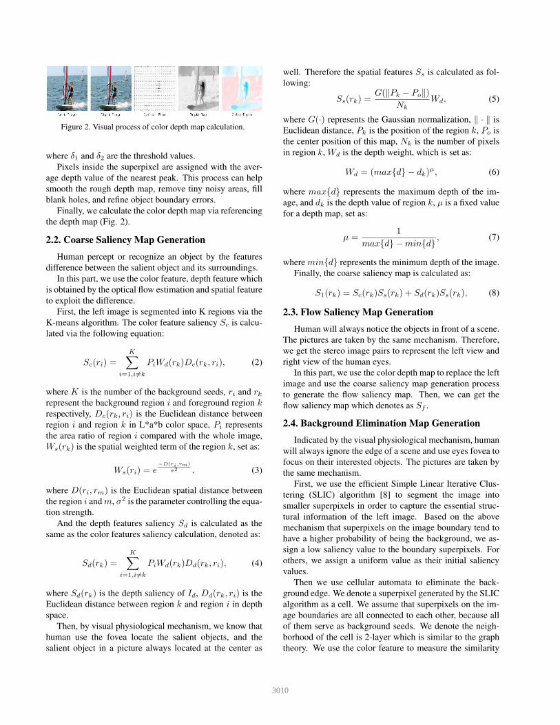
Figure 2. Visual process of color depth map calculation.
where δ1 and δ2 are the threshold values.
Pixels inside the superpixel are assigned with the aver-
age depth value of the nearest peak. This process can help
smooth the rough depth map, remove tiny noisy areas, fill
blank holes, and refine object boundary errors.
Finally, we calculate the color depth map via referencing
the depth map (Fig. 2).
2.2. Coarse Saliency Map Generation
Human percept or recognize an object by the features
difference between the salient object and its surroundings.
In this part, we use the color feature, depth feature which
is obtained by the optical flow estimation and spatial feature
to exploit the difference.
First, the left image is segmented into K regions via the
K-means algorithm. The color feature saliency Sc is calcu-
lated via the following equation:
Sc(ri) =
K∑
i=1,i 6=k
PiWd(rk)Dc(rk, ri), (2)
where K is the number of the background seeds, ri and rkrepresent the background region i and foreground region krespectively, Dc(rk, ri) is the Euclidean distance between
region i and region k in L*a*b color space, Pi represents
the area ratio of region i compared with the whole image,
Ws(rk) is the spatial weighted term of the region k, set as:
Ws(ri) = e−D(ri,rm)
σ2 , (3)
where D(ri, rm) is the Euclidean spatial distance between
the region i and m, σ2 is the parameter controlling the equa-
tion strength.
And the depth features saliency Sd is calculated as the
same as the color features saliency calculation, denoted as:
Sd(rk) =
K∑
i=1,i 6=k
PiWd(rk)Dd(rk, ri), (4)
where Sd(rk) is the depth saliency of Id, Dd(rk, ri) is the
Euclidean distance between region k and region i in depth
space.
Then, by visual physiological mechanism, we know that
human use the fovea locate the salient objects, and the
salient object in a picture always located at the center as
well. Therefore the spatial features Ss is calculated as fol-
lowing:
Ss(rk) =G(‖Pk − Po‖)
Nk
Wd, (5)
where G(·) represents the Gaussian normalization, ‖ · ‖ is
Euclidean distance, Pk is the position of the region k, Po is
the center position of this map, Nk is the number of pixels
in region k, Wd is the depth weight, which is set as:
Wd = (max{d} − dk)µ, (6)
where max{d} represents the maximum depth of the im-
age, and dk is the depth value of region k, µ is a fixed value
for a depth map, set as:
µ =1
max{d} −min{d}, (7)
where min{d} represents the minimum depth of the image.
Finally, the coarse saliency map is calculated as:
S1(rk) = Sc(rk)Ss(rk) + Sd(rk)Ss(rk), (8)
2.3. Flow Saliency Map Generation
Human will always notice the objects in front of a scene.
The pictures are taken by the same mechanism. Therefore,
we get the stereo image pairs to represent the left view and
right view of the human eyes.
In this part, we use the color depth map to replace the left
image and use the coarse saliency map generation process
to generate the flow saliency map. Then, we can get the
flow saliency map which denotes as Sf .
2.4. Background Elimination Map Generation
Indicated by the visual physiological mechanism, human
will always ignore the edge of a scene and use eyes fovea to
focus on their interested objects. The pictures are taken by
the same mechanism.
First, we use the efficient Simple Linear Iterative Clus-
tering (SLIC) algorithm [8] to segment the image into
smaller superpixels in order to capture the essential struc-
tural information of the left image. Based on the above
mechanism that superpixels on the image boundary tend to
have a higher probability of being the background, we as-
sign a low saliency value to the boundary superpixels. For
others, we assign a uniform value as their initial saliency
values.
Then we use cellular automata to eliminate the back-
ground edge. We denote a superpixel generated by the SLIC
algorithm as a cell. We assume that superpixels on the im-
age boundaries are all connected to each other, because all
of them serve as background seeds. We denote the neigh-
borhood of the cell is 2-layer which is similar to the graph
theory. We use the color feature to measure the similarity
3010

among cells. If a neighbor has more similar color with the
cell, it will have a bigger impact on the cell at next moment.
We define the influence factor between the cell i and the cell
j as:
Fij =
{
Ws(ri) , j ∈ Nb(i)
0 , j /∈ Nb(i), (9)
where Nb(i) is the neighbor set of i.
The next moment of each cells’ status is controlled by its
current status and its neighbors’ status, so, we need to bal-
ance the influence of these two aspects. At the same time, if
there are more similar characteristics among current cellular
and its neighbors, the probability which they all belong to
the foreground objects or background area is bigger, there-
fore, the neighbors should have an enormous effect on the
current cells. So, we can constantly reinforce the effect of
the foreground seed and assimilate the neighbor cells which
have the similar color with current cell. In this way, we can
calculate more salient objects. To measure the influence of
a cell by its neighbors, we use confidence matrix C to rep-
resent the influencing process, which is denoted as:
Ci = a×Ci −min(Cj)
max(Cj)−min(Cj)+ b, (10)
where i is the current cell, j its neighbors. The initial value
of confidence matrix Ci equals to the reciprocal of the max-
imum of influence factor Fij . The parameters of a and bcontrol the range of confidence matrix.It can be seen from
the definition of confidence matrix that the more similar be-
tween the current cell i and its is neighbors j, the smaller
value the confidence matrix Ci will have at index (ij). Pa-
rameter b represents the prescribed influencing minimum.
And the parameters of a and b should satisfy the following
formula:
a+ b < 1, a ≥ 0, b ≤ 0, (11)
We consider that the case where the parts of salient ob-
jects will have the enormous difference in the color feature,
so, the parameter a can not be set too large. In this paper,
the parameters of a and b are set to 0.6 and 0.2 respectively.
By setting the range, we can ensure that each cell is auto-
matically updated to a more stable and accurate state.
Finally, we use the synchronous update rule shown in
Eq.(12) to get the background elimination saliency map
(BES). We denote it as Sb which is calculated by the fol-
lowing:
St+1 = CSt + (I − C)FSt, (12)
where C is the confidence matrix, I is the identity matrix,
and F is impact factor matrix. St is the saliency value of
the current state which is calculated by Eq.(2).
2.5. Final Saliency Map Generation
After obtaining the coarse saliency map S1, the flow
saliency map Sf and the background elimination saliency
map Sb. We can get the final saliency map S of the left
image via the fowling equation:
S = SbSfS1. (13)
The main steps of the proposed salient object detection
algorithm are summarized in Algorithm 1.
Algorithm 1 The proposed saliency detection algorithm
Input: stereo image pairs I;
Output: final saliency map S;
1: generate the depth maps Id use the Optical Flow;
2: for each region k = 1,K do:
3: compute color saliency values Sc(rk) via Eq.(2) and
depth saliency values Sd(rk) via Eq.(4);
4: calculate the center-bias and depth weights Ss(rk) via
Eq.(5);
5: get the coarse saliency map S1 via Eq.(8);
6: end for
7: obtain flow saliency map Sf and background elimina-
tion map Sb;
8: figure out the final saliency map S via Eq.(13) ;
9: return final saliency map S;
3. EXPERIMENTS
We evaluate our method on our SSD100 dataset,
NJU2000 dataset [6], RGBD1000 [10] dataset and
RGBD135 [3] dataset, and compare the results with the
state-of-the-arts. More experimental analyses on the effec-
tiveness of our method are given as follows.
3.1. Datasets
Our SSD100 dataset is built on three stereo movies. The
movies contain both the indoors and outdoors scenes. We
pick up one stereo image pair at each hundred frames. It to-
tally has tens of thousands of stereo image pairs. We make
the image acquisition and image annotation independent to
each other, we can avoid dataset design bias, namely a spe-
cific type of bias that is caused by experimenters unnatural
selection of dataset images. The chosen stereo image pairs
are based on one principle: choose the one which the com-
puter detect the salient objects within the complex scenes
where even the human cannot tell the salient objects at once.
After picking up the stereo image pairs, we divide the image
pairs into left images and right images both in 960 × 1080size. When we build the ground truth of salient objects,
we adhere to the following rules: 1) we mark the salient
objects, taking the advice of most people; 2) disconnected
3011

Figure 3. Examples of the proposed SSD100 dataset. From top to bottom: left-view images, right-view images, depth maps, ground truth.
Figure 4. Visual comparison of saliency maps on four datasets.
3012
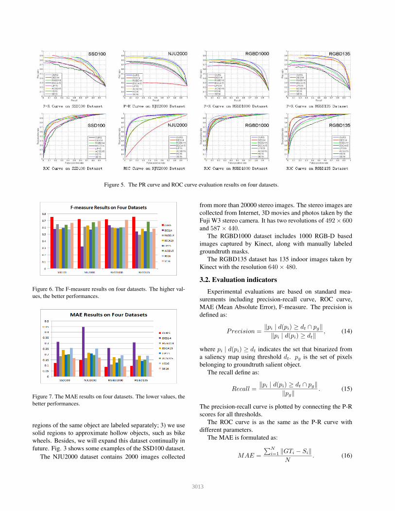
Figure 5. The PR curve and ROC curve evaluation results on four datasets.
Figure 6. The F-measure results on four datasets. The higher val-
ues, the better performances.
Figure 7. The MAE results on four datasets. The lower values, the
better performances.
regions of the same object are labeled separately; 3) we use
solid regions to approximate hollow objects, such as bike
wheels. Besides, we will expand this dataset continually in
future. Fig. 3 shows some examples of the SSD100 dataset.
The NJU2000 dataset contains 2000 images collected
from more than 20000 stereo images. The stereo images are
collected from Internet, 3D movies and photos taken by the
Fuji W3 stereo camera. It has two revolutions of 492× 600and 587× 440.
The RGBD1000 dataset includes 1000 RGB-D based
images captured by Kinect, along with manually labeled
groundtruth masks.
The RGBD135 dataset has 135 indoor images taken by
Kinect with the resolution 640× 480.
3.2. Evaluation indicators
Experimental evaluations are based on standard mea-
surements including precision-recall curve, ROC curve,
MAE (Mean Absolute Error), F-measure. The precision is
defined as:
Precision =‖pi | d(pi) ≥ dt ∩ pg‖
‖pi | d(pi) ≥ dt‖, (14)
where pi | d(pi) ≥ dt indicates the set that binarized from
a saliency map using threshold dt. pg is the set of pixels
belonging to groundtruth salient object.
The recall define as:
Recall =‖pi | d(pi) ≥ dt ∩ pg‖
‖pg‖. (15)
The precision-recall curve is plotted by connecting the P-R
scores for all thresholds.
The ROC curve is as the same as the P-R curve with
different parameters.
The MAE is formulated as:
MAE =
∑Ni=1
‖GTi − Si‖
N. (16)
3013

where N is the number of the testing images, GTi is the area
of the ground truth of image i, Si is the area of detection
result of image i.The F-measure is formulated as:
Fmeasure =2× Precision×Recall
Precision+Recall. (17)
3.3. Comparison
To illustrate the effectiveness of our algorithm, we com-
pare our proposed methods with DES14 [3], RGBD14 [10],
BSCA15 [11], LPS15 [7], ACSD15 [6], HS16 [12] and
SE16 [4]. We use the codes provided by the authors to re-
produce their experiments. For all the compared methods,
we use the default settings suggested by the authors. And
for the Eq. (3), we take σ2 = 0.4 which has the best contri-
bution to the results.
Fig.5 shows PR curve and ROC curve comparison results
on four datasets.
Fig.6 and Fig.7 show F-measure comparison results and
MAE comparison results on four datasets, respectively.
From the comparison results, we can see that our
saliency detection results have a better robustness results on
four datasets. Besides, we also show the visual comparisons
as shown in Fig. 4, which clearly demonstrate the advan-
tages of the proposed method. We can see that our method
can detect salient objects more precisely. In contrast, the
compared methods may fail in some situations.
4. Conclusion
In this paper, we proposed a biologically motivated
saliency detection framework for automatically produc-
ing saliency map from stereo image pairs. We imitate
the processing of the human visual perception to gener-
ate a framework which composes of background elimina-
tion part, color flow detection part and features difference
saliency part. Besides, we build a new high-quality dataset
with complex scenes based on dataset design principles.
The experimental results on four datasets demonstrate our
algorithm improves the quality of saliency detection and is
more robustness. To encourage future works, we make the
SSD100 dataset and related materials open. All of these can
be found on our project website1.
5. Acknowledge
We would like to thank anonymous reviewers for theirhelpful comments on the paper. This work was supportedby the grant of National Natural Science Foundation ofChina (No.U1611461), the grant of Science and Tech-nology Planning Project of Guangdong Province, China(No.2014B090910001) and the grant of Shenzhen PeacockPlan (No.20130408-183003656).
1https://chunbiaozhu.github.io/prof.cbzhu/
References
[1] M. Bjrkman and D. Kragic. Active 3d segmentation through
fixation of previously unseen objects. In British Machine
Vision Conference, BMVC 2010, Aberystwyth, UK, August
31 - September 3, 2010. Proceedings, pages 1–11, 2011.
[2] M. M. Cheng, N. J. Mitra, X. Huang, and S. M. Hu.
Salientshape: group saliency in image collections. Visual
Computer, 30(4):443–453, 2014.
[3] Y. Cheng, H. Fu, X. Wei, J. Xiao, and X. Cao. Depth en-
hanced saliency detection method. 55(1):23–27, 2014.
[4] J. Guo, T. Ren, and J. Bei. Salient object detection for rgb-d
image via saliency evolution. In IEEE International Confer-
ence on Multimedia and Expo, pages 1–6, 2016.
[5] L. Itti. Automatic foveation for video compression using a
neurobiological model of visual attention. IEEE Transac-
tions on Image Processing A Publication of the IEEE Signal
Processing Society, 13(10):1304–1318, 2004.
[6] R. Ju, Y. Liu, T. Ren, L. Ge, and G. Wu. Depth-aware salient
object detection using anisotropic center-surround differ-
ence. Signal Processing Image Communication, 38(C):115–
126, 2015.
[7] H. Li, H. Lu, Z. Lin, X. Shen, and B. Price. Inner and inter
label propagation: salient object detection in the wild. IEEE
Transactions on Image Processing A Publication of the IEEE
Signal Processing Society, 24(10):3176–3186, 2015.
[8] A. Lucchi, K. Smith, R. Achanta, G. Knott, and P. Fua.
Supervoxel-based segmentation of mitochondria in em im-
age stacks with learned shape features. IEEE Transactions
on Medical Imaging, 31(2):474–86, 2012.
[9] N. Ouerhani and H. Hgli. Computing visual attention from
scene depth. In International Conference on Pattern Recog-
nition, page 1375, 2000.
[10] H. Peng, B. Li, W. Xiong, W. Hu, and R. Ji. RGBD Salient
Object Detection: A Benchmark and Algorithms. Springer
International Publishing, 2014.
[11] Y. Qin, H. Lu, Y. Xu, and H. Wang. Saliency detection via
cellular automata. In Computer Vision and Pattern Recogni-
tion, pages 110–119, 2015.
[12] J. Shi, Q. Yan, L. Xu, and J. Jia. Hierarchical image saliency
detection on extended cssd. IEEE Transactions on Pattern
Analysis and Machine Intelligence, 38(4):717–729, 2016.
[13] D. Sun, S. Roth, and M. J. Black. Secrets of optical flow esti-
mation and their principles. In Computer Vision and Pattern
Recognition, pages 2432–2439, 2010.
[14] C. Zhu, G. Li, X. Guo, W. Wang, and R. Wang. A Multi-
layer Backpropagation Saliency Detection Algorithm Based
on Depth Mining, pages 14–23. Springer International Pub-
lishing, Cham, 2017.
[15] C. Zhu, G. Li, N. Li, X. Guo, W. Wang, and R. Wang. An
innovative saliency detection framework with an example of
image montage. In ACM MultiMedia Workshop 2017 Sub-
mission Proposal for South African Academic Participation
Proceedings, 2017.
[16] C. Zhu, G. Li, W. Wang, and R. Wang. Salient object de-
tection with complex scene based on cognitive neuroscience.
In Multimedia Big Data (BigMM), 2017 IEEE Third Inter-
national Conference on, pages 33–37. IEEE, 2017.
3014