A Thickness Design Method for Concrete Pavements

A. C. ESTEP, Engineer of Design, and PAUL I. WAGNER, Assistant Engineer of Design,

California Division of Highways

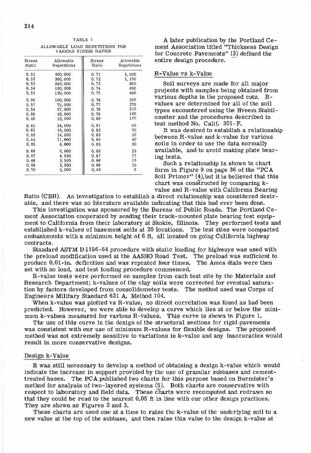
The thickness of portland cement concrete pavement and the underlying cement-treated layer was formerly based on Cali­fornia's Traffic Index, which was developed for use in flexible pavement design. Because the Traffic Index is computed from all predicted truck axle loadings, its use is not necessarily valid for rigid pavement designs. A design method was adapted from previous design work published by the Portland Cement Association, and adjusted empirically to fit past experience with satisfactory concrete pavements. A new method of predicting truck traffic from loadometer data and classified truck counts was developed. The design method is sensitive to variation in support value of the underlying soil, thickness of granular sub­base, thickness of cement-treated base, modulus of rupture of the concrete, and truck traffic predicted for the design life of the pavement.

•THE design of pavements and their supporting layers is recognized as a gray area in­habited by specters of uncertainty and ghosts of old broken pavements. The only guid­ing light is past experience, which may be partially obscured by incomplete records of road life and maintenance.

Uncertainties result because it is often cheaper to overdesign instead of investing a large sum in an exhaustive soil survey. Engineers know that it is uneconomical to pro­cess natural deposits until aggregates have the uniformity of a factory product. They have experienced the frustrations that occur when 'trying to get uniform compaction on a project with varying soil types, bad weather, or inexperienced personnel.

The worst uncertainty is the prediction of future traffic that will use the pavement during its design life. Even if reliable classified truck counts are available on existing high­ways in the area, there are problems of assignment of this traffic to the new facility and expansion of the assigned traffic to the total volumes expected during the design period.

Despite the difficulties cited, it is not believed desirable to leave the determination of the structural elements of the roadbed entirely to rules in a manual or to the judg­ment of individuals. Engineering judgment is a necessary element in all good design, but in the interest of consistency and uniformity a definite design method should be used as a basic tool. Departures from the results of the strict use of a design process will have to be made on some individual projects, but such modifications should be justified in each instance.

California has adhered to these principles for many years in the design of flexible pavements, but the thicknesses of portland cement concrete pavements have been se­lected by a set of rules. In recent years, thicknesses were chosen that corresponded

Paper sponsored by Committee on Rigid Pavement Design. . 212

213

to the depths of standard side forms. With almost all concrete pavement construction in the state now being performed by the slip-form method, there is no reason to be limited to any particular pavement thickness.

Previously, concrete pavement thickness and depth of cement-treated base was de­termined by rule from California's Traffic Index. The Traffic Index is calculated from total 5000-lb equivalent wheel loads, and this total is computed from estimated future truck traffic using axle weights of all trucks. This is an acceptable process in flexible pavement design, but it is not necessarily valid for rigid pavement determinations, which should be based only on those loads that produce a stress ratio in excess of 0. 50. In this context, stress ratio is the stress produced by a given load divided by the modulus of rupture of the concrete determined by third-point loading at 28 days.

In the selection of concrete pavement thickness from the Traffic Index, no adjust­ment was made for variation in the support value of the natural soils encountered un­less they were expansive. When the soils were expansive, the granular subbase layer was increased to provide sufficient weight in the total structural section to prevent fu­ture expansion of the underlying material with resulting loss in stability.

A design method was desired that would be sensitive to the support value of any nat­ural materials that might be found when the soil survey was made for each project, and also would show the increase in support provided by the use of subbases and cement­treated bases. A minimum 0. 50-ft thickness of granular subbase has been used when the R-value of the underlying soil is less than 40. Cement-treated bases have been used under nearly all concrete pavements for about 20 years. The purpose was to pre­vent erosion of the subgrade by pumping, and to provide extra support at the joints.

Another objective was to have a design method that would use the same loadometer data, soil survey reports, and classified truck counts used for flexible designs. Such a method would not be limited in range, and could result in either thicker or thinner designs than were previously considered. This would enhance the validity of the eco­nomic comparison made to determine the choice between rigid and flexible pavement for a given project.

After review of the literature, it was concluded that the simplest approach to devel­oping a concrete design method would be to adapt the design data previously published by the Portland Cement Association to the traffic and soil survey information available for all California highway projects. It was also indicated that one or more factors in the new design method would have to be empirically adjusted to correlate the new de­signs and past experience with satisfactory concrete pavements.

DESIGN METHOD DEVELOPMENT

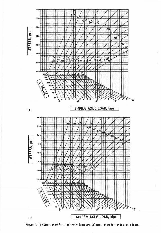
Fordyce and Packard (1) proposed a concrete highway pavement design procedure based on three major elements: analysis of stress due to moving loads, fatigue result­ing from stress ratios exceeding 0, 50, and load safety factors. They had prepared charts for single and tandem axle loads that gave stress relationships to axle loads, k­values (Westergaard's modulus of subgrade reaction), and slab depths. These charts were based on influence charts developed by Pickett and Ray (2) from Westergaard's theoretical analysis of concrete slab behavior. In order to use these stress charts, it was proposed to develop a procedure for determining k-values from the soil survey data obtained for each project. This will be discussed later in detail. The stress charts reproduced here as Figure 4 and Figure 5 have been redrawn with slab thickness lines for 0,05-ft increments instead of '/2-in. increments. This was done to corre­spond to our standard practice of designing depths of flexible pavements and the under­lying layers to the nearest 0. 05 ft. This eliminates the need of converting inches to feet in quantity, profile, and construction staking calculations.

Fordyce and Packard (1) had proposed a new PCA fatigue curve for concrete pave­ments subject to flexural stresses. From this curve they had prepared a table of al­lowable stress repetitions to failure vs stress ratio as previously defined. This table was extended from the curve and used without further modification. It is presented here as Table 1.

214

Stress Ratio

o. 51 0. 52 o. 53 0. 54 0. 55

0. 56 o. 57 0. 58 o. 59 0. 60

o. 61 0. 62 o. 63 o. 64 o. 65

o. 66 o. 67 o. 68 o. 69 0. 70

TABLE 1

ALLOW ABLE LOAD REPETITIONS FOR VARIOUS STRESS RATIOS

Allowable Repetitions

400, 000 300, 000 240, 000 180, 000 130, 000

100, 000 75, 000 57, 000 42, 000 32, 000

24, 000 18, 000 14, 000 11, 000

8, 000

6, 000 4,500 3, 500 2, 500 2, 000

Stress Ratio

o. 71 o. 72 o. 73 0. 74 0. 75

0.76 0. 77 o. 78 o. 79 o. 80

o. 81 0. 82 0.83 0,84 o. 85

o. 86 o. 87 o. 88 o. 89 0.90

Allowable Repetitions

1, 500 1, 100

850 650 490

360 270 210 160 120

90 70 50 40 30

23 17 13 10

8

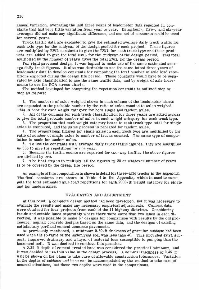
A later publication by the Portland Ce­ment Association titled "Thickness Design for Concrete Pavements" (3) defined the entire design procedure. -

R-Value vs k-Value

Soil surveys are made for all major projects with samples being obtained from various depths in the proposed cuts. R­values are determined for all of the soil types encountered using the Hveem Stabil­ometer and the procedures described in test method No. Calif. 301-F.

It was desired to establish a relationship between R-value and k-value for various soils in order to use the data normally available, and to avoid making plate bear­ing tests.

Such a relationship is shown in chart form in Figure 9 on page 36 of the "PCA Soil Primer" (4),but it is believed that this chart was constructed by comparing k­value and R-value with California Bearing

Ratio (CBR). An investigation to establish a direct relationship was considered desir-able, and there was no literature available indicating that this had ever been done.

This investigation was sponsored by the Bureau of Public Roads. The Portland Ce­ment Association cooperated by sending their truck-mounted plate bearing test equip­ment to California from their laboratory at Skokie, Illinois. They performed tests and established k-values of basement soils at 20 locations. The test sites were compacted embankments with a minimum height of 6 ft, all located on going California highway contracts.

Standard ASTM D 1196-64 procedure with static loading for highways was used with the preload modification used at the AASHO Road Test. The preload was sufficient to produce 0.01-in. deflection and was repeated four times. The Ames dials were then set with no load, and test loading procedure commenced.

R-value tests were performed on samples from each test site by the Materials and Research Department; k-values of the clay soils were corrected for eventual satura­tion by factors developed from consolidometer tests. The method used was Corps of Engineers Military Standard 621 A, Method 104.

When k-value was plotted vs R-value, no direct correlation was found as had been predicted. However, we were able to develop a curve which lies at or below the mini­mum k-values measured for various R-values. This curve is shown in Figure 1.

The use of this curve in the design of the structural sections for rigid pavements was consistent with our use of minimum R-values for flexible designs. The proposed method was not extremely sensitive to variations ink-value and any inaccuracies would result in more conservative designs.

Design k-Value

It was still necessary to develop a method of obtaining a design k-value which would indicate the increase in support provided by the use of granular subbases and cement­treated bases. The PCA published two charts for this purpose based on Burmister's method for analysis of two-layered systems (5). Both charts are conservative with respect to laboratory and field data. These Charts were recomputed and redrawn so that they could be read to the nearest 0.05 ft in line with our other design practices. They are shown as Figures 2 and 3.

These charts are used one at a time to raise the k-value of the underlying soil to a new value at the top of the subbase, and then raise this value to the design k-value at

.. ...

z

'

400

V> "300 0.. .. ; ::> ...J

~ 200

100

10

215

/ ,,,/

~v --~ ~

zo l O 40 50 60 70 BO

R - VALUE

Figure 1. k-value vs R-value.

the top of the cement-treated base. If no subbase is used because of high k-value for the basement soil, just the second chart (Fig. 3) is used to obtain the design k-value.

Estimated Axle Load Repetitions

Loadometer surveys are made every year in California and truck counts, classified by the number of axles, are also made on a statewide basis.

Data from these two sources are used to compute total estimated 5000-lb equivalent wheel loads (EWL) for each project for a 20-year design period extending ahead from the estimated date of project completion. Traffic index is derived from this total EWL figure and used in the design of flexible pavements.

In developing EWL constants from loadometer data, it had been found expedient to use California Table W-4, All Main Rural and Urban (reproduced in the Appendix as Table 2), because the differences in truck traffic patterns between main rural and urban were insignificant for state highways. It also had been determined that despite

100

600

400

:WO

6a$111111 1oil : JOO k ot ,.::.::.=-r- I

I, soil ,zoo_ ~

-i.--

1000 900 BOO

z 700

~ 600 ... .,; 500

"'

• oO .-~-;~O" - -\ . ·- -

~ --- _,,-!!!!!!f-I

' zoo : 400

·VF-::; .io -o'Y

,, 1. ,bi / ~ c .. ... ill ... ~ 100

e .. 0

20

L--.-"I" jOO L---

~ ' , ---- --1 ! 50 .......-~"~-~

10'~ -~ O 0.1 02 O.J 0.4 05 06 07 0 .8 0.9 1,0

THICKNESS OF SUBBASE - FEET

Figure 2. Effect of various thicknesses of granular subbases on k-values.

.. ~ 500 c ... "' ... ' 5 200

~ ... 0 ... 0 100 ... z 0

50

; _ ..... ~oi . QO/ .......-

; / ,,,~...- .,,....-

v ,y>r ~ ./ ~o ;' / 1.~-?" ,.-

/ V' v / /

/

/v 0 0 I 0 ,2 03 0 .4 0.5 0 .6 0,7 08 09 10

THICKNESS OF CEllENT-TREATED BASE , FEET I

Figure 3, Effect of various thicknesses of cement­treated bases on k-values.

216

annual variation, averaging the last three years of loadometer data resulted in con­stants that had very little variation from year to year. Usingfour-, five-, and six-year averages did not make any significant difference, and one set of constants could be used for several years.

Truck traffic data are expanded to give the estimated average daily truck traffic for each axle type for the midyear of the design period for each project. These figures are multiplied by EWL constants to give the EWL for each truck type and these prod­ucts are added to give the total EWL for the midyear of the design period. This total multiplied by the number of years gives the total EWL for the design period.

For rigid pavement design, it was logical to make use of the same estimated aver­age daily truck figures. It also was desirable to use the same latest three years of loadometer data to develop constants for computing the total number of axle load repe­titions expected during the design life period. These constants would have to be sepa­rated by axle classification to use the same traffic data, and by weight of axle incre­ments to use the PCA stress charts.

The method developed for computing the repetition constants is outlined step by step as follows:

1. The numbers of axles weighed shown in each column of the loadometer sheets are expanded to the probable number by the ratio of axles counted to axles weighed. This is done for each weight category for both single and tandem axles.

2. All of the columns for each truck classification for three years are added across to give the total probable number of axles in each weight category for each truck type.

3. The proportion that each weight category bears to each truck type total for single axlP.s is computed, and the same process is repeated for tandem axles;

4. The proportional figures for single axles in each truck type are multiplied by the ratio of number of single axles to number of trucks counted. The same type of compu­tation is made for tandem axles.

5. To use the constants with average daily truck traffic figures, they are multiplied by 365 to give the repetitions for onP. yP.a.r.

6. Because the traffic counts are reported for two-way traffic, the above figures are divided by two.

7. The final step is to multiply all the figures by 20 or whatever number of years is to be covered by the design life period.

An example of this computation is shown in detail for three-axle 1trucks in the Appendix. The final constants are shown in Table 4 in the App-endix, which is used to com­pute the total estimated axle load repetitions for each 2000-lb weight category for single and for tandem axles.

EVALUATION AND ADJUSTMENT

At this point, a complete design method had been developed, but it was necessary to evaluate the results and make any necessary empirical adjustments. Current data were obtained for four projects from each' of the 11 highway districts. Considering inside and outside lanes separately where there were more than two lanes in each di­rection, it was possible to make 57 designs for comparison with results by the old pro­cedure, asphalt concrete designs based on the same data, and the designs of existing satisfactory portland cement concrete pavements.

As previously mentioned, a minimum 0.50-ft thickness of granular subbase had been used when the R-value of the underlying soil was less than 40. This provides extra sup­port, improved drainage, and a layer of material less susceptible to pumping than the basement soil. It was decided to continue this practice.

A O. 35-ft depth of cement-treated base was considered the practical minimum, and it was decided to use this value in the design proce.RR. A nominal thickness of 0,45 ft will be shown on the plans to take care of allowable construction tolerances. Variation in the depths of subbase and base can bP. accommodated by the method to take care of unusual situations, but these two depths were used in the comparisons.

217

Safety factors are usually used in concrete pavement design, and these have been referred to as load impact factors. Fordyce and Packard (1) suggest that in reality they are load safety factors and that term is used here. They suggested values ranging from 1.0 to 1.2 depending on the type of street or highway and the expected truck traf­fic characteristics. These same load safety factors are shown in the PCA's "Thickness Design for Concrete Pavements" (3).

These load safety factors were used in the first trial designs to evaluate the new method. The comparison showed lighter designs than had been used in pavements with a satisfactory road life of 20 to 35 years before resurfacing or replacement. An ad­justment had to be made, and it was decided that changing the load safety factors was the best way to accomplish this since these factors are empirical judgments.

The load safety factors and types of facility finally were designated as follows:

LSF = 1.3 for the outside lanes of Interstate highways and other multilane projects with high predicted truck traffic;

LSF = 1.2 for the inside lanes of Insterstate highways and other multilane projects with high predicted truck traffic, and for all lanes of projects with moderate predicted truck traffic; and

LSF = 1.1 for minor highways, frontage roads or streets with low predicted truck traffic.

In the PCA publications, the 1. 0 value is suggested for residential streets or rural roads carrying similar traffic. This category is outside state highway practice, and our adjustment expanded the two higher traffic categories to three classifications.

Another adjustment was made in the axle load values used to enter the stress charts. Originally the average value of the load increment was used, but this did not result in designs as heavy as past experience indicated were necessary. Using the top value of the increment, as shown in the PCA method, gave the desired results when combined with the increases in the load safety factors.

The final comparison indicated close agreement with many past designs using O. 75-ft depth of concrete pavement. In the heaviest traffic patterns for which O. 67-ft thick­ness had been used, the new method indicated 0. 75-ft despite a 0.10-ft increase in the depth of cement-treated base. For the heaviest truck traffic reported, the new depth of pavement would be 0.80 ft. Finally, the new method provided a procedure for de­signing thinner pavements for lighter traffic patterns than had been considered previ­ously for the use of portland cement concrete pavement.

DESIGN PROCEDURE

The project data required for the design process are the type of facility, number of lanes, minimum R-value of the basement soil, expected modulus of rupture of the con­crete, and estimated average daily trucks for the midyear of the design period. With these data, the design procedure consists of the following steps, listed in order:

1. Determine the k-value of the basement soil. 2. Find the increased k-value due to the use of a granular subbase. 3. Determine the k-value at the top of the cement-treated base. 4. Choose a load safety factor and apply it to the design axle loads. 5. Select a trial thickness of pavement, and determine the stresses for each axle

load for both single and tandem axle loads. 6. Compute the stress ratios by dividing each stress value by the modulus of rup-

ture of the concrete. 7. Record the allowable ax~e load repetitions for each stress ratio. 8. Compute the estimated numbers of axle load repetitions for the design period. 9. Determine the percent each estimated number of repetitions bears to the allow­

able repetitions, and add these values to obtain the total percent fatigue resistance used.

218

Several pavement thicknesses should be tried and that trial thickness selected which shows the nearest to 100 percent fatigue used, but not to exceed 125 percent. The 125 percent upper limit is allowed because a change of 0.05 ft in pavement thickness results in a large change in percent fatigue used, and also because a conservative approach was used throughout the development of the method. Examples of this are the use of minimum k-values, the determination of modulus of rupture from 28-day specimens with third-point loading, and the use of high load safety factors.

To make it easy to follow the design procedure, an example is worked out in detail in the Appendix.

SUMMARY

This new method of portland cement concrete pavement design is sensitive to all of the variables now reflected in California's flexible pavement designs. It uses the same soil survey data, predicted truck traffic, and loadometer survey data. It provides structural sections that result in more valid economic comparisons with flexible de­signs for selection of pavement type. It produces designs that are nearer optimum and this should result in some economies. It provides extra thickness where unusual con­ditions of foundation or traffic are encountered.

It is believed that the adoption of this method of rigid pavement design eliminates the inadequacies of designing by arbitrary rules and raises the professional level of California's structural design activities.

REFERENCES

1. Fordyce, Phil, and Packard, R. G. Concrete Pavement Design. Presented to AASHO Committee on Design, October 22-25, 1963.

2. Pi~kett, GeraJcl, and Ray, Gordon K. Influence Charts for Concrete Pavements. Trans. ASCE, Paper No. 2425, Vol. 116, p. 49-73, 1951.

3, Thickness Design for Concrete Pavements. Concrete Information, HB 35, Port­land Cement Association, 1966.

4. PCA Soil Primer. SCl0-3, Portland Cement Association, 1962. 5. Burmister, D. M. The Theory of Stresses and Displacements in Layered Systems

and Applications to Design of Airport Runways. HRB Proc. Vol. 23, p. 126-148, 1943.

Appendix PROCEDURE FOR COMPUTING LOAD REPETITION CONSTANTS

The following example, which is shown for three-axle trucks only, illustrates the procedure for computing load repetition constants. The expansion of loadometer data is further limited to the year 1965, but the method is the same for each year of load­ometer data used.

1. A portion of a loadometer Table W-4, All MR and U, is reproduced here, desig­nated as Table 2. All three-axle truck columns are used and these are marked (A), (B), and (C). The numbers of axles weighed in the current column are expanded by the ratio of axles counted to axles weighed. In column (A), this would be 2805 divided by 765 equals 3. 66667 for both single and tandem axles. This probable number factor is multiplied by the sum of the numbers of axles under 16 kips and each following number in the column. The figures are entered in column (7) on the work sheet designated Table 3. The same computation is made for tandem axles and the process is re­peated for columns (B) and (C ), using the appropriate probable number factors, and entered in columns (8) and (9). The same type of calculation was made for the years 1963 and 1964 and entered in columns (1) to (6) in Table 3.

219

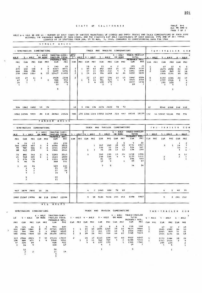
2. The horizontal lines are added across to give the total probable numbers of axles in each weight category. These sums are recorded in column (10).

3. The proportion that each weight category of single axles bears to each single ax­le truck type total is computed, and the same process is repeated for tandem axles. In column (10), the first figure, 30,807.6, is divided by 32,586.0, and the quotient, 0.94542, is recorded as the first figure in column (11). This is repeated Ior every figure in col­umn (10) for single axles. For tandem axles the divisor would be 6687.0.

4. The proportional figures for single axles in each truck type are mUltiplied by the ratio of number of single axles to number of trucks counted. In this example from col­umn (10), 32, 586 would be divided by 15, 320 to give a factor of 2.12702. This factor multiplied by the proportional figures in column (11) gives the products recorded incol­umn (12) fo1· each weight category. The same type of computation is made for tandem axles, dividing 6687 by 15, 320.

5. To use the constants with average daily truck traffic figures, they are multiplied by 365 to give the repetitions for one year.

6. Because the traffic counts are reported for two-way traffic, the figu1·es are di­vided by two. Steps 5 and 6 are combined and all of the figures in column (12) are mul­tiplied by 365 divided by 2 and recorded in column (13).

7. The final step is to multiply all of the figures by 20 or whatever number of years .is to be covered by the design life period. These final constants are shown in column (14).

The final constants for all truck types and weight categories are shown in Table 4, which is used to compute the total estimated axle load repetitions for each 2-kip incre­ment of axle loading.

DESIGN PROCEDURE

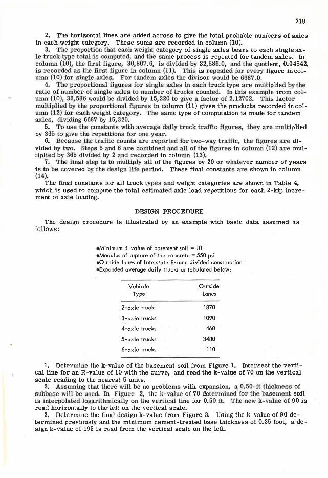
The design procedure is illustrated by an example with basic data assumed as follows:

•Minimum R-value of basement soil= 10 •Modulus of rupture of the concrete= 550 psi •Outside lanes of Interstate 8-lane divided construction •Expanded overage daiiy trucks as tabulated below:

Vehicle Outside Type Lanes

2-axle trucks 1870

3-axle trucks 1090

4-axle trucks 460

5-axle trucks 3480

6-axle trucks 110

1. Determine the k-value of the basement soil from Figure 1. Intersect the verti­cal line for an R-value of 10 with the curve, and read the k-value of 70 on the vertical scale reading to the nearest 5 units.

2. Assuming that there will be no problems with expansion, a 0. 50-ft thiclmess of subbase will be used. In Figure 2, the k-value of 70 determined for the basement soil is interpolated logarithmically on the vertical line for 0.50 ft. The new k-value of 90 is read horizontally to the· left on the vertical scale.

3. Determine the final design k-value from Figure 3. Using the k-value of 90 de­termined previously and the minimum cement-treated base thiclmess of 0,35 foot, a de­sign k-value of 195 is read from the vertical scale on the left.

220

TABLE 2

s J H 6 l E A X l E S

18 Kl P AX.LE S I N G L E U N 1 T TRUCKS TRAC TOR AXLE LOADS IN EOUIVALENCY F ACJO POUNDS ANO li!I RIGID Flf>l 18LE •ANEL - PICKUP 2 - AXLE, 2 - AJlLE, (~)_ A•LE I SINGLE UNIT (B) I IC.JP AXLE EQUI- PAVEMENT PAVEMENT UNDER ONE TONI . - TIRE 6 - ru:E . - Anf. lRUtKS TOlAL ' - ll!U . -Vlll:NCV ITEMS P=2.5 P 2 l. 5

cUARENT"" 'PRiOR 0•9 SM•5 CUil PR! CUR PRI CUR PRI CUR PR I CUR PRI CUR PRI CUR

UNOER 3000 0.0002 0 .. 0002 7"'2 o\7111 293 •11 621 '19 5 I L L61t30 l 06930 I) 3 • 3000- 6999 0.005 0.005 966 487 220 23' o\lo\9 lo\14 2H ... o\1357 H"23 917 669 332 1000- 7999 o.026 0.032 • 2 2 5 550 361 135 119 )025 2834 HI 268 197 8000--11999 0.08Z o.os1 I 2 • 1106 lZO 216 195 5'i190 5127 720 504 J18

1200C-15999 o.Jo\1 O.l6ll I '18 301 8• ., • H89 2057 H9 269 172 I 1600C l BODO o. 783 0.196 I 139 ., 15 19 688 676 109 03 I 07

1M001-20COO 1.260 l.Zo\O •• 25 3 2 206 161 30 24 Z) 20001-21999 J..916 l.8Z6 1 5 1 • l5 2 I

22000-21999 2.818 2.su 2 12 I 2.\000-25999 3.976 3.531 2600C--29999 6.Zl'f 5.38Cll 3000\1-3'11999 11 .. 395 9.'t32

TOTAL SINGLE AXLES WE: IGHEO IOl't 5272 520 ••o 7121 51,.,. 165 5H • 2511 1830 1220

TOTA.L SI hGLE AllLES C.lJUfrHEO Z2952 lU24 9 ... 0 SO lit 14llt2 12224 2805 2579 12 1• 169901 151455 10662 10~15 5b24

i /CAl IF LEG.AL LIMIJ. SIHGl. E ... u 11000 POUNDS JAHD•" • A l e '

lA llCJP lltf s I N G L E U N I T T " U C K S TRACTOR AXLE LOADS IN EQUI YM. ENC.V fAC. T"" P:.JUNOS ANO 19 RIGID FLEX IBLE 'iNEL - PICKUP 2 - AXLE, 2 - iXLE,

iKLE I -S I NGLE UH i T I KIP ULE E~I PAYElltENT Pi YE MENT UNDE!lt ONE TONI . - TIRE . - TJRE 3 - . - A)C U ••ucu rnuL J - ULE 4 - I VAU:NC.Y nu•s Pz2.5 P•2., 'J ··---c-- ··--· 0•9 SN•5 CUil PRI CUR ••• CUR PRI CU• ... CUR PR I CURI' ENT PRIOll CUR ••• tu•

UNOEll bllOO 0.010 0.010 5 2 18 10 16 t:l00-11999 CaOlO 1).010 26• 161 910 108 219

l2000--17<';19'J 0 .. 062 o.o,.,. 224 146 821 106 118 130'10-23CJqq 0.253 o. 1'8 ,. 1l >71 ... lH

24Cmc-29q99 c. 729 0.426 9' 62 3'5 300 93 l 30000-::JlOOIJ l .. 305 O .. J'J] •• 51 2•9 2'6 30

12001-13999 1 .. 100 C .. 910 28 25 103 121 1 3400G-J59q9 z.165 1.230 6 • 22 20 2

16000- J 1999 2.721 l.5 :H i 38000--3999~ 3.313 l .. 8tl5 I 2 11 I 40000-41999 't.129 2.289 I • 42000-'t3999 't.997 2 .. J'tq I 5

4400(1-'t5999 ~ .. 9117 1 .. 001 41i0QC-49999 1 .. 125 41 .. 170 l 5 50000-54999 10 .. 160 s .. 100

fOfAl fAHOtM AlllLES WEIGHED 705 53) l. 610

TOTAL TANDEM AJCLES COUNTED 2805 257• 6 1 ZIUl 2586 2812

UCAL IF LEGAL lflillT. TANDEM AllllE~ )2000 POUNDS A l L A Jj, L E S

U KIP AIU: S J N G L E U N I T T • u c • s TRACTOR -AXLE LOADS IN EQUl'fAL.fNtY FACTOR PWNUS AND 119 •IGJO FLEKIBLE PANEL - PICKUP 2 - AXLE, 2 - AKLEt SINGLE UNIT Kl' &"Lt fQUI- PAYElltUH PAYFMNT I UNDER o• TOIO . - TIAE t. - TIRE 3 - AXLE . - AXLE TRUCKS TOTAL ' - AXLE 4 - .. VAlOKY ITE'IS P•2•' , .. 2 .. 5 PROBABLE lt!IOS ..

0•9 SN•5 cuo '"' CU• PU cu• ,., CU• ••• CUR PRI CUfUlENT PRIOR CUR PRI CUR

UNDER 1000 1 ... 2 •111 203 '11 621 ... 26 • 116'507 l069M 13 3 .. )000- 6tt9 966 U1 220 114 ... , )•14 •o~ 559 417115 35407 917 66• 871 100(>-- 7999 • 2 2 • no 3'1 291 220 1596 ll22 HI 268 204 1000--11999 1 2 • 1106 720 591 4'5 7109 6517 720 504 607

120UO-lS•99 •11 301 115 259 3Z7o\ 1082 ,.. 26• 102 l 16000 18000 IH " 90 •• 9•2 1045 10• 93 1•8

JIOOl-20000 •• 25 10 6 232 19• 30 ,. 30 20?01-21999 l • • • 5• ' l

22000-2.34)99 22 24000-25'999 261)00-29999 10000-34999

STATE OF CALIFORNIA

221

TABLE W-lt All "R ANO U PAGE 7 Of 1

AtllE W-4 IAll MR ANO UI-- NUMBER Of AXLE LOADS Of VARlOU S MAGNITUDES Of LOA.OED AND EHPTY TRUCtl:S ANO TRUCK C0"1BINATIONS OF EACH rYPE WEIGHED, THE PROBABLE NUMBER OF SUCH LOADS, ANO THE EI GHTEEN KIP AXLE EQUIVALENTS OF EACH GENE~Al TYPE ANO OF All TYPES

COUNTED AT 19 STATIONS FROM JUN. 15 10 .. UG. 5, l9b5, COMPARED TO CORRESPONDING DATA FOR 196.lt

SINGLE AXLE S

- SEMITRAILER C DMBI NAT IONS TRUCK AND TRA lLER COP181NATIONS TWO-Tst.All e • c 0 "

6 - AXLE fRAtr OK--S E1"1 - ((j)_ Allf I • - UL E

6 - AXLE lRUC.K-U,Al lER ~

lllLE ' - AXL E. QA KORE fRAI LER TOUL 5 - AX,LE OR "OA.E TOTAL ~ - Al( I r. . - .... . - .... P',.VQ-"Olt. l"l.V;a • "•Uo•o.- ""'"

PRI CUR PRI CUR PRI CUR PRI CUR PRI CUR PR! CUR PR! CUR PRI CUR PRI CUR PR! CUR PRI CUR PR!

3 ff I l HO 45 16 4 10 6 z l 93 ,. I 61 12 • 5

215 132 106 ) 8 616] 60ll l I 65 63 892 658 14 I 7 551t5 'Slq2 l 2679 2080 51 33 168 394 284 I 't609 lt396 l 11 II 28) Z3 2 • 5 1641 l6q6 z l085 869 22 16 ZS9 l't02 lOH • 15 12411 11493 2 I 24 24 79• 609 42 34 lt38Z •634 1506 1191 •9 30

135 23 11 I 2.\08 2338 2 Z2 11 251 194 10 15 16 .. 2 l 554 s 1150 106.ft 20 17 61 z I I 906 90Z I • II 701 5Z5 l I 3515 3llt'5 I 1151 1526 z 6 26 I Z39 ,,. 3 6 Z3S 175 ll 17 1236 299 zzo 2

I 13 5 2 I 10 7 5 5 I

• I

934 1962 1440 10 20 12 3 156 136 3114 2400 78 1Z 12 85't8 6968 148 110

4960 10586 9933 88 118 26960 25526 964 no 13<\6 ll64 l ~552 16248 ZB .,, 18105 18139 132 56 53442 51164 790 134

fAHOEl'I AX:L fS

- SEMITAAI LU COMB I MT IONS TRUCK ANO TRA lLER C.OM6 INATI ONS T W 0 - J R A I l e R c 0 "

6 - AXLE TRAC.TOR-SEMI-U'.LE I .. - 6 - AX~E -rRUCK.- TAAfLEA

... -· .. 'f ••• f 5 - .... \E nA -·• lllAIL<A 'ft • • ' UL E 'i" - AXl ir:' UA l'IDRE TOT AL 4 ... t•L~ 5 - ••• • " -PA.08ADlE NOS . l'f\UDA.QL I:. nu.11.

PRI CUA PRI CUR PRI CUR PRI CUR PR I CUR PR! CUR PR! CUR PR! CUA PR I CUR PR! CUR PM! CUR PR!

• H 11 l 253 110 2 3 5 20 I 2 166 1033 667 I 9 6646 5523 l 341 Z60 28 20 1711 l"HC' ) I .. 1 9• nz 466 6 3131 31b1 100 12 14 5 526 5ZO 10 6 88 '12 ,.. 4 2800 25'tl I I 26 28 11 12 114 288 7 6

7) 891 740 J 4 5295 5510 3 249 183 13 24 1258 13CJ6 6 1 2 Zl S48 405 I l 3123 2909 238 184 4 4 ll 75 1272 l 2 I

5 216 118 I 1531 1259 Bl 59 396 400 I I 5 66 16 368 551 12 9 I 59 61

I 21 16 123 lib l 5 34 34

3 • 21 2 7 5 2 21 .. 3 I 16 7

• 2Z 2 11

••l 3819 2810 10 26 4 2 1060 800 78 69 6 I 40 35

2480 21067 19796 •• 118 23967 2239.ft • 3 8 518.ft 5416 205 '53 5398 5~01 9 3 241 212

ALL A.Cl ES-

SEMITRAILER COM8IN,&TIONS TRUCK ANO TRAILER COMB I NAT I CNS r • o - R A I L E R t o H

6 - AXLE TRACTOR-SEMI- 6 - AXLE TRUCK-TRAILER

lE 5 - AlllE OR "ORE TRAIL Ek TOT Al 3 - AXLE 4 - AXLE 5 - AXLE OR MURE TlJTAL 4 - AXLE - AXLE 6 - AXLE PR08A8LE NOS. PROBARLE NOS.

PR! CUR PRI CUR PRI CUR PRI CUR PRI CUR PRI CUR PRI CUR PR! CU• PR I CUR PR! CUR PR! CUR PR!

24 124 64 I 3 944 600 16 4 15 8 8 q ,,. l4P. I 6 1 12 1 10 661 2681 l86l 8 ,. 22521 20322 65 6 5 169" 1245 79 60 9613 CJ484 3 2685 ZOBZ 84 so 252 , .. 544 l 4 6 962 664CJ 11 11 341 219 18 • 191t0 2044 ? l00 5 869 31 21 ••1 2566 1910 10 28 20276 18752 28 26 903 709 •• 65 "'~ 5543 1506 ll 9\ 66 4•

ll3 2546 2026 10 l7114 17227 26 11 lllO 82R 42 60 5922 6145 l l 0:3 1064 J8 19 104 884 615 4 594t8 5761 9 II Q62 137 l 4788 '5216 1760 15.lb 2

37 124 89 938 922 3 6 270 103 1346 1366 29• no I 16 • 100 61 I 1• 7 5 s

lZ 70 2 II 14 l 5

5

222

TABLE 3 CALCULATIONS OF CONSTANTS FOR LOAD REPETITIONS FOR 20 YEARS FOR ONE VEHICLE -ADT (TRUCKS)

~ LOAOOW ETER SURYEY DATA TABLE W- 4 Al l llR a U PROBABLE NUMBERS -(I} 12} (JI ,.,, (51 (GI "' (8/ (9/ lw (l/J f/21 I/JI ""' TRUCK tl ASS 3· 4XLE

YEAR / ?'3 / ?''f' /, .... _ TOTAL PRO· uf7,,z .1£u x

IPROO. HO. FACTOR .a.hr.II ~. 3/0.J. • .,,,,.7 .-..,, ...... , ~'J'J7~Z l.U4D~ '~"''? ,J...,.,,/ .. £1,.d()"""' PORTIO" 2"

U1'dU 16 ,,. ,,. OO•Q ....., ,,_,.,,,,, .,, .. ~~ ,. ,. .1.• ···- !f/1141.:17.~ A 'J .e- 16 - 18 S:2. ~7-Z 17.> ..,.,.n 7J. ~ .Ni~ ·""/-'2 ,, a•z 0U3.<I• ~ 18-20 i .u 2. .4' ~z ' • <7 //." /,'9 - "'/a~ ~A,JIJ ~~7' ,,.~

g W-22 "'' ~..- ,----L,li " ,. '-l'f/ .. ,. .. 3 22-24 .... 24-26 .... 26- 28 >< .. 28cJO .... .... 30-32 "' z 32- 34 u; 34-35

TOTAL PROBABLE NO l/!110 4-:Z2/0 ,,fJ.O 2<13.0 972,,,, 211.0 Z8tJ£o V"''2.o JIM .5Zf4(o .l.1MJ7d P 212702 ',1841.!1;. ,,,:J_,~

PROB. NO. FACTOR 2 . ..f,f.J/ - - -- _,,,,,_r.,, - -- '.1'""7 -- - - - - ~ l;-LI• - -Undu Z:4 8J.J.A - - zo.:11.tJ 201•.• .#.,.,,,/ iJ. 'Nlf.?> OJZJ°1' ~~.,f~ ,,,.•./.H 24-26 .,.u """ / / -#,<f 2>1.o IA.d,,.,. -. P/~~/ ?. tJ8~1 U, 7n - 26- 28 _,,,,,,,. "'·" :/#,~ 2,f~IJ I A .. ,,,, A,d/~'f/ ·~,, ,. ,_ ?:U.

z 28-30 ..,.,. 9/ .1 /,/~, .I1f.• • A,JIJ,~J ~11.,/& il"..:111 J.t1,il . .IU ~~~.It .. 30-32 /P~.P Z /J . ./ N~:

.57/.# 4d#.F.T/ d.(1•7.1.• L 1/p~ /.3'-iZI~ .. 32-34 __fi,!_. /11/.IJ 2 6.1." 4 h/~/ . L'-~7tJ ~ 34-36 / .2.,, 2 i· 42..IJ .n.• "·""""' O.lld3?A ''"'"~ ' ·' · 7.-,: ~ 36-38 ~ z.,, d.OlftJ'1 ~ ddd/7 O.d J / O 0 . 620 ... 38-40 2, ~-

.,,, (!.dQ/P6 ~o"~'

,,,,,,,., /, "' "'

~ 40·42 Z.{. ,,,, 7:2.

._,,_, AMO /. 7//.

Q 42-44 - ,,,, ,,., '°'.A#(l~t dda/I' " o.11.rµ /.1111. ..

44 - 46 - -~ -46-48 ~· Z.J d,Jl(JP ... ,,,,,,,,,$" Q.IJ:l,7..,. .. .r~· 48 - 50 .2..3 ,.,, A AAO W.. ~HQ/.J t?..OZ "T<• <?NA

TOTAL PR0,8ABLE NO, 1177tJ -- -- 2,85.• - - Z81f5:0 -- -- ,,,,.. 1'.01100• 11, ..... 11.,? ,,,,.rr6 '5p.l,2.

TOTAL AXLES .ff ?'"

TOTAL VEHICLES / 5.3ZO

IABLE 4

CALCULATIOH OF 20-YEAR AXLE LOAD REPETITIOH5

Oisl.-Co.-Rte. t:JO-XX-Q(/ P .M. lflt?/P'-'1 Exp . Auth . Qt?(lt210 Inside Lanes __ _ Outside Lanes _K___

Axle 2-Axle 3-Axle 4-A:de S-Aale 6 -Aale T utal

Lo•d• ADTT = /870 ADTT = /O~O ADIT = -11~0 ADIT = 3'f#IO ADIT = //0 20-year

Kips Const•nt Repetition• Con•t•nl RepeUtion• Con•t•nt Repetition• Con•t•nt Repetition• Con•t•nl Repet l tions RepetitionM

35 0.09 .9/A .flU~

34 0.17 ...f'Y.JI -~· w 32 0 . 17 .< ... • SYJ ...J 30 14.3 /_....,. . ./_4'7.• x <( 28 14.l °J.rl.I ./ .:S-7.t w 26 28.7 JL~7 .7./-"' ...J Cl 24 1.75 ti • • • 3.72 / '?// 0 .44 / llr», I&·'/" z v; 22 5.91 .//Ar'I 3.10 ~-.,... 9.20 ~--· 6.28

.,,_,,,,.,,. 27.4 .. ,,,,,~ --.-~,

20 40 .4 ----· 86 9 --··· 202. .,,. _,,

419. ,,,. _ _,,i,,

60.4 18 128. 334. 611. 2060. 349.

so I\ J 0.55 .&JN. 0.55 /Y.. - ,4

48 ' / 0.55 "" ... 0.55 /19, .J 46 ' / --- I. SO ..r~ ~ ..

w 44 ' / l .10 / ,, J4 1.75 ii& ~ ., __,

42 ' / l ,72 /• 3.80 ... .. '·' x <( 40 / 1.72 / 5.66 2• • 3.29 ,,./ .. ~

,, ,, ~ 38 x 0.62 4 -9.09 -- J 22.6 .. ,. 28.8 J/~ ~~ w 0 36 ' 13.8 L4" 12.1 ' ~· 78.3 ""' '7 61.4 ~7.' ...... -z <( 34 / \. 62.7 ~~- II 35.4 JL 262. .,,,, :...i 62. 9 ' ....

\. 32 / 136. 145. 576. '¥12 . 30 / ' 6i.7 lf.4. 292. 462 . 28 / \. 61 .7 164. 292. 462. 26 ,

' 61.7 164. 292. 462.

223

4. For this example, a load safety factor of 1. 3 is appropriate for outside lanes. On the work sheet (Table 5), the axle load designations in column (1) are multiplied by 1.3 and the resulting figures are entered to the nearest 0.1 kip in column (2).

5. Stresses are determined from Figure 4 (a) for single axle loads and Figure 4 (b) for tandem axle loads. A trial thickness of pavement is first selected and then the charts are entered with each axle load in column (2) of the work sheets. The load line is followed to the horizontal line for the design k-value, thence vertically to the trial thickness line, and then horizontally to the stress scale on the left. The stress values are entered in column (3) of the work sheet to the nearest 5 psi.

To illustrate from the example, a trial depth of O. 75 ft was chosen for the outside lanes. The first axle load in column (2) is 45.5 kips. \This value is interpolated in Figure 4 (a) and followed up to the combined k-value of 195 which also must be interpo­lated. From this point proceed vertically to an intersection with the O. 75-ft curve, thence horizontally left to the scale where a stress of 370 psi is read and recorded on the work sheet. Stresses are determined for each axle load in column (2) for single axles, and in the same manner for tandem axles using Figure 4(b).

TABLE 5 WORK SHEET

Dist.-Co.-Rte. 00 -X X-OO P.M. 0.0 / 00.0

Outside Lanes __g__ Inside Lanes ___ Exp. Auth. 000000

Load Safety Factor (L.S.F. ) __ /._.3 __ Basement Soil R-Value_'"""/_O _ _

Subbase Depth O. 6""0' Cement -treated Base Depth 0. .,_.5'"

k-Values: Basement _ __LO _Subbase ___ ';O ___ c.T.B. / ~_S __ _

Modulus of Rupture (M.R. ) _ _ .S:_ "'.5i_ 'O __ Trial Depth PCC __ O.::_. L.Z,_'S_" _ _

(1) 2) 3) (4) (5) ( 6) (7) Axle Axle Stress Stress Allowable Estimated Fatigue Load Load Ratio Repetitions Repetitions Resistance

x L.S.F. Col. 3 Used M.R:-

Kip a Kips . psi No. No. ;, SINGLE AXLE LOADS

, . ~- ..:> 70 I." 7 - on " : ~

... Lo 2 ,~ ·o I. t' 'll _,,

-~ • ' .. '" 5 .. r

"'> I. ' •t. I , ll'l /.< ~

2 ..,.[ .,,,. , tr. /$ .. i' _J;JJ , ~ /.J l ; 'A-'l ~ I.

;. j_ 2,11; I.~ _,._,, ',, ),1) b.5. ~

!R.• .2E.i < l a - _:_ -&.. I)

1 J ··~

TANDEM AXLE LOADS c;o ~ .r.o r.6ln I ,,,;;; /t', (. I 1n p~, .. -'"'"' ll ~ "'' rl)

l "' '1~ , ,, ,-'l ,; _,r ...... ... 1

~ '...:~, I _ ..... ?I. ... , , ,, . _;; ,,, , /nl '""' ·~ J ., '~

~ '"' .. ,. /p; ;o; 10 ,.,.. ;, .. ,1

•n . , ,,.,, /~ 4 'J'J - --,, """' .... ~'~ , - --,, ..... r

-. ... ~

" " -. .1 {,

? 1 4

Total % Fatigue Used 80

en a.. en-en LI.I ct: I-en

(al

en a..

en en LI.I ct: I-­en

(b)

600 I '

550

eoo

4!10 I " i..r',

,, / /

400

,, . ~ -;;i~ .r ,

" I/ (/ ,, ..

/ ,, " I

350 / ,, j ,oi! , ~ ,,, v

I .I

-·~

300 , .... I II

250 f / I/ ~

•psi,"

SINGLE AXLE LOAD, kips

600 ,,. /

,,, ,. ,, ,, ,. , I/

I '

!100 'n ••

~ .r . ' ~c;:

I " , (/ I/

II , ,. / 450 I I I I ,,..

~ / / v I/ I/

400 II

I l/ ,. , (/

I/ ,, v , ,. ,,. I ,. 3!10

.... "7' 7f:",. . s

1-~ -e-, 4)'- I- 'O, ot -r..fo 'i a o 0.1 ,1.,t..J,o I ,. 300

II I I / , / ,. I , ,.

• .,., .. o .!, 0 0

!IOO

•o;,., \ \ I'\ '\ ' ' "" ' ''" ~r-.; ...:-~"' 200' \r\I\ \'\ l\.~r-.M"'~:;:;:':S::::::::::i::::

"- 1ao r\I\ V' I\ '" '-'."' , .... t-;:::: ~ ' I\ \ \' l\r-. I\.\ "'

,, ~:::: ~::::: t"-"' .... :::::::

~ '"" '\ \\ \\' \ '' ,,,~,,,~ .... ,,,,~~ (1' 10 '\i\ ~l\'\ ' \~,~~~,~r,','~~ ~~ ............. \ ..... :::-,.....,~,...

50 I\ ,, I\. , .... ' '

.~ .. ·~··, ..... ii, ... ~ .. , ' VI ~ ~ .. •

2!10

0 • .o

TANDEM AXLE LOAD, kips

Figure 4. (a) Stress chart for single axle loads and (b) stress chart for tandem axle loads.

225

6. Each stress value is divided by the modulus of rupture (MR) and the ratios re­corded to the neai·est 0.01 in column (4) of the work sheet. No values less than 0.51 are used because allowable repetitions are unlimited for stress ratios of O. 50 or less. It can be seen from this that no stress values less than half the modulus of rupture need be determined in the preceding step.

7. Allowable repetitions are taken from Table 1 for each stress ratio and recorded in column (5 ).

8. Estimated numbers of axle load repetitions for 20 years are calculated on the form represented by Table 4. For this example, the expanded average daily trucks for each vehicle type are entered in the column headings. The average daily truck figure for each vehicle type is multiplied by each constant for that type and the repetition fig­ure entered to the right of the constant. By adding the repetition figures on each hori­zontal line, the probable number of repetitions for each weight classification is ob­tained. The total 20-year repetitions are then entered in column (6) on the work sheet, Table 5.

9. For the final step, the estimated repetitions in column (6) are divided by the al­lowable repetitions in column (5) and multiplied by 100, which gives the percent fatigue resistance used. These figures are recorded to the nearest one percent in column (7) of the work sheet. Column (7) is totaled and the total percent fatigue used is recorded. Several thicknesses are tried and that trial thickness is selected which shows the near­est to 100 percent fatigue used but not to exceed 125 percent. With experience only two trials are necessary.

In this example, only the calculations for the finally selected design thickness of 0, 75 ft for the outside lanes are shown to illustrate the method. A trial thickness of O. 70 ft also was used, but this lesser thickness showed a "fatigue resistance used" far in excess of 125 percent.