1

____________________________________________________________________________________________________

A Thermodynamic Approach to Monetary Economics – A Revision An application to the UK Economy 1969-2006 and the USA Economy 1966-2006

____________________________________________________________________________________________________

John Bryant VOCAT International Ltd, 10 Falconers Field, Harpenden, AL5 3ES, United Kingdom. E-mail: john.bryant@vocat.co.uk Abstract: This paper develops further monetary aspects of a model, first set out as part of a paper by the author published in 2007, concerning the application of thermodynamic principles to economics. The model is backed up by statistical analysis of quarterly data of the UK and USA economies. The model sets out relationships between price, output volume, velocity of circulation and money supply, and develops an equation to measure entropy gain in an economic system, linked to interest rates. This paper was first released in August 2008, but has now been revised to reflect current thinking. Keywords: Monetary, thermodynamics, economics, entropy, interest rates

JEL Classification: E, E4, Y8

Biographical notes: John Bryant is director of VOCAT International Ltd, a company specialising in economic consultancy and research, and expert witness services. His prior career appointments have included group economist and manager corporate planning for multi-national corporations, and economist and investment analyst for a stock broking group. He first became interested in the relationship between economic theory and the laws of thermodynamics in 1974, and has published several papers on the subject since that time, culminating in a key paper published in 2007 [Bryant, J. (2007)]. ____________________________________________________________________________________________________

1. Introduction and Equation of State This paper expands on and improves a monetary model set out in a previous paper by the author [Bryant, J. (2007)]. In that paper an ideal equation for a money flow system was given by: NkTPV= (1)

Where P is the price level, V is output volume, N is the number of currency instruments in circulation, k is a nominal monetary standard (£1, €1, $1, etc) and T is an Index of Trading Value (or velocity of circulation). This equation is a re-statement of the general quantity theory of money PY=MV, where P is price level in an economic system, Y is output in volume terms, M is the quantity of money in circulation (variously defined as M0 – M4, but with M4 generally being recognised as a standard), and V is the velocity of circulation. While the left-hand sides of the equations are comparable, the right-hand side requires additional clarification. To obtain an exact comparison with the quantity theory, equation (1) can be written as [ ]TNkPV= (2)

Where Nk is equivalent to money M in circulation and the index of trading value T in a thermodynamic monetary system is equivalent to the velocity of circulation V in a traditional monetary system. To avoid any confusion concerning the use of algebraic symbols the quantity theory equation PY=MV is dispensed with in this paper. The above equation has the same format as the thermodynamic Ideal Gas Equation PV=NkT, where P is pressure, V is volume of gas, N is the number of molecules of gas, k is the Boltzmann constant and T is the temperature. Samuelson (1970) acknowledged that the relationships between pressure and volume in a thermodynamic system bear a striking similarity in terms of differentials to price and volume in an economic system; and Pikler (1954) has highlighted the connections between the velocity of circulation and temperature.

February 2010

2

At this stage we are not pre-forming a view on how the factors inter-relate, and whether they follow a Monetarist, Keynesian or other school of thought. All that can be confirmed is a tautological identity, with a change in one or more of the factors automatically equating to a balancing change in the others, in a manner so far undefined. All of the factors can vary, and none can be considered to be constant. A point to note with a monetary model is that the velocity of circulation T, calculated as output in value terms divided by money supply, carries a connotation of value too, since the nominal value k is unchanging, and the number N of monetary instruments is just that – a number. If the number of monetary instruments N in circulation remains constant, when output price P and output volume V are each changing in some fashion, then the changes in P and V are reflected in a change in the velocity of circulation T. T therefore carries value as well as volume. This is not to say of course that the number of money instruments N necessarily remains the same. Thus there are four variables to consider, and in differential form equation (1) can be written as:

TdT

NdN

VdV

PdP

+=+ (3)

Figure 1 illustrates the trend of economic development of the UK and USA economies. UK data is taken from quarterly statistics of Economic Trends Annual Supplement (www.statistics.gov.uk). USA data is taken from quarterly statistics of www.federalreserve.gov and www.bea.gov. Volume data is taken from GDP chain volume measure [UK 2003 prices, USA 2000 prices]. The Price deflator is calculated by dividing GDP at market prices by the volume measure. The raw data was smoothed by calculating 4-quarter moving averages.

Figure 1 Annualised percent growth rates of key economic variables

GDP Deflator (P), Output Volume (V), Money Stock (N) [UK M4, USA M3], and Velocity of Circulation (T)

UK Economy

-20

-15

-10

-5

0

5

10

15

20

25

30

1969 Q3 1973 Q3 1977 Q3 1981 Q3 1985 Q3 1989 Q3 1993 Q3 1997 Q3 2001 Q3 2005 Q3

% p

er a

nnum

.

dP/PdV/VdT/T (M4)dN/N (M4)

USA Economy

-10

-5

0

5

10

15

1966q1 1970q1 1974q1 1978q1 1982q1 1986q1 1990q1 1994q1 1998q1 2002q1

% p

er a

nnum

.

dP/P

dV/V

dT/T (M3)

dN/N (M3)

3

A particular problem with a money system, compared to an energy system, is that whereas in the latter the value k is defined as a constant, being energy per molecule per degree of a scale of temperature, which can be derived by experiment, in a money system, inflation can have the effect of reducing the effective value of money. The nominal fixed amount k remains the same, but the effective real value of money can decline. However, when viewed from the point of view of the money instrument k, it sees itself as unchanging (£1, €1 etc), but all around it is changing. Technology effects, such as replacement of cash by plastic and electronic transfer, can also change the velocity of circulation, most marked obviously with respect to the M0 definition of money. History abounds with attempts to derive an unchanging standard, such as gold, man-hours and energy content. A less dramatic but still important issue is that of the definition of output volume V, given that over long periods of time the mix of goods and services changes, entailing sophisticated deflator estimates to try to strip inflation out and take into account switches from high volume low added value to low volume high added value. Last, calculation of the velocity of circulation is by definition a residual exercise, being equated to total output at market prices divided by total money instruments, rather than being set against an independent scale. Technical changes in the usage of money can also occur, altering the velocity of circulation. The combination of these problems makes for a more complex analysis. 2. Development and Elasticity Before developing a thermodynamic representation of a money system, a point should be made concerning the number of variables. In a non-flow thermodynamic system, both the constant k and the number of molecules N are fixed, and there are therefore only three variables left to consider, pressure P, volume V and temperature T. In a thermodynamic flow system, on the other hand, there are four variables left (other than the constant k): molecular flow N, volume flow V, pressure P and temperature T, but these are effectively reduced to three, by replacing volume flow V and molecular flow N with specific volume v = V/N. Thus again only three variables remain, enabling thermodynamic analysis to proceed. However, in a money system, all five factors can vary. Although the money value k is constant (i.e. £1, $1), this is only thus in nominal terms. A period of extensive inflation can reduce its effective value. Thus dividing a real output flow V by the money stock number N still leaves four variables. Moreover, dividing a volume output by a number of units of a depreciating currency might negate the principle of defining output at constant prices. As the relative level of volume output per unit of time also defines to a large extent the size of an economic system, preserving the integrity of volume flow V is important. By way of illustration, in the UK between 1969 and 2006 money stock grew by a factor of 59, output volume by a factor of 2.4 and prices by a factor of 11.7; in the USA between 1966 and 2006 money stock grew by a factor of 21, output volume by a factor of 3.3 and prices by a factor of 5. Compensating adjustments in the velocity of circulation accounted for the remainder. It is inconceivable that technical change adjustments equated to inflation. To develop the thermodynamic analysis it is necessary to reduce the four variables in equation (3) to three, preferably without losing output volume V. A monetary system is essentially a flow system with a circular component, and its size is described by output volume, like a balloon getting larger, and sometimes smaller. It has some similarities to thermodynamic flow systems. A possible part solution to this problem is to transpose the price deflator P to the right hand side of the equation, to derive a Specific Money Stock NP= N/P, leaving output volume V alone on the left hand side. This arrangement, though acceptable, does not accord with standard presentations of thermodynamic analyses, or of general economic practice of having both price and volume flow on the output side of the equation. A subsidiary problem to consider, however, is the extent to which changes in price P reflect loss of currency value k, or gains in real value. This all rather depends upon from where an observer is standing in order to view an economy and its surrounding economies. All is relative, though some factors might be more relative than others. Nevertheless, the net effect of using this method will likely be to understate money entropy change and this point should be born in mind all through this paper. The probability is that any change in money instrument stock N may find its way into changes in all three of the other variables, price, output volume or velocity of circulation, depending upon the relative elasticity between the three and with money, and the degree to which a money system is out of kilter with the stable state, such as the existence of excess money or high inflation. In this paper, therefore, the preferred arrangement to convey the thermodynamic characteristics is to transpose money units N to the left-hand side of the equation, and divide output price level P by the number N of monetary units in circulation to give a Specific Price PN(=P/N). Presentations of the inverse NP (= N/P) are also given in this paper however for completeness.

4

Thus equation (1) could be written as: kTVPN = (4) And differentiating, and dividing by PNV=kT we have:

TdT

VdV

PdP

N

N =+ (5)

Where (dPN/PN) also equals –(dNP/NP). Figure 2 illustrates the relationships between the factors.

Figure 2 Velocity of Circulation, Specific Price and Output Volume

For an economy where no change in output volume occurs (V = Constant), increases/decreases in specific price PN are matched by an equivalent change in the velocity of circulation T. Such changes in specific price PN involve a change in the relationship between actual price level P and the money stock N. At the other extreme, where no change in the specific price PN occurs, changes in real output volume V are matched by appropriate changes in the velocity of circulation T. Should a movement in money supply N occur, this will be balanced by a change in price P. If the velocity of circulation T remains constant, then any change in output volume V will result in an offsetting change in the specific price PN, accompanied by a change in the relationship of price P to money supply N. A change in velocity of circulation T can arise either from a change in specific price PN or a change in output volume V, or both. And no change in the velocity of circulation T will occur if a change in specific price PN is balanced by an equivalent change in output volume V. Figure 3 illustrates the relationships in more detail.

Output Volume V

Specific Money Stock

NP (=N/P)

(=1/PN)

Specific Price PN (=P/N)

(=1/NP)

Velocity of Circulation T

Output Volume V

Velocity of Circulation T

5

Figure 3 Specific Price – Output Volume relationships

Last, a further relationship between the variables can exist, which in this book we have called Polytropic case (PNVn = Constant), involving an Elastic Index n, where changes in all of the factors can take place, but in a complex manner. The polytropic equation (PNVn = Constant) can be adapted to meet all of the possible processes. A constant specific price process (dPN/PN=0) for example is a polytropic process with the elastic index n set at zero, and a constant volume process is one with the elastic index set at ± infinity. The iso-trading model (PNV=Constant) has an index of 1, with no change in velocity of circulation T. By combining equation (5) with the polytropic equation (PNVn = C), the following equations describe the polytropic case:

n

N

N

VV

PP

−

⎟⎟⎠

⎞⎜⎜⎝

⎛=

1

2

1

2 ( )VdVn

PdP

N

N −= (6)

nn

N

N

PP

TT

1

1

2

1

2

−

⎟⎟⎠

⎞⎜⎜⎝

⎛=

N

N

PdP

nn

TdT

⎟⎠⎞

⎜⎝⎛ −

=1 (7)

n

VV

TT

−

⎟⎟⎠

⎞⎜⎜⎝

⎛=

1

1

2

1

2 ( )VdVn

TdT

−= 1 (8)

Thus far, we have not specified how the relationships impact on the way in which an economy moves and what drives the relationships, only that changes in one or more of the factors will be reflected by changes to the others to enable the equation of state set out at equations (1), (3) and (5) to balance out. Figures 4a and 4b illustrate the trend of the relationships for the UK and USA economies, making the adjustments to PN = P/N, as per equations (6), (7) and (8).

Specific Price PN (= P/N=1/NP)

V = Constant

Output volume V

PNV n = Constant

PN = Constant

PNV = Constant

6

Figure 4a Quarterly data Specific Price, Output Volume and Velocity of Circulation

UK Economy (M4)

0

1

2

3

4

5

0 0.5 1 1.5

Output Volume V £trillion 2003 prices

Spec

ific P

rice

Pn (=

P/N

)

1969

1982

1972

1991

2006

Velocity of CirculationT = 2

T = 1

UK Economy (M4)

0.0

0.5

1.0

1.5

0.0 0.5 1.0 1.5

Output Volume V £trillion 2003 prices .

Spec

ific M

oney

Np

(= N

/P) (

£tril

lion

2003

pric

es)

2006

1991

1969

Velocity of Circulation T = 1

T = 2

A trend line drawn through the curve at figure 4a for the UK economy is of the form PNV2.0=1.1, with a regression of R2=0.96. This result, however, masks the significant disturbances brought about by the large inflationary boost in the period 1972 to 1982. More relevant results are obtained by dividing the trend into segments:

• 1969-1972 PNV2.28 = 0.86 (R2=0.89) • 1972-1982 Result not significant (R2=0.06) • 1982-1991 PNV2.62 = 0.91 (R2=0.98) • 1991-2006 PNV1.53 = 1.11 (R2=0.98)

A trend line drawn through the curve at figure 4a for the USA economy is of the form PNV1.097=1.73 with a regression of R2=0.97. This result, however, masks a 5-year change in the relationship 1989 to 1994 when growth in money supply N declined and velocity of circulation rose, before settling back to the original path. More relevant results are obtained by dividing the trend into segments:

• 1966-1989 PNV1.28 = 2.26 (R2=0.99) • 1989-1994 PNV-0.64 = 0.057 (R2=0.91) • 1994-2006 PNV1.98 = 12.74 (R2=0.97)

7

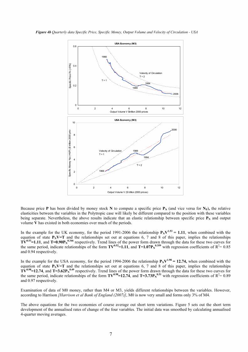
Figure 4b Quarterly data Specific Price, Specific Money, Output Volume and Velocity of Circulation - USA

USA Economy (M3)

0

0.2

0.4

0.6

0 2 4 6 8 10 12Output Volume V $trillion 2000 prices

Spec

ific P

rice

Pn (=

P/N

)

1966

1989

1994

2006

Velocity of CirculationT = 2

T = 1

USA Economy (M3)

0

2

4

6

8

10

0 2 4 6 8 10 12

Output Volume V ($ trillion 2000 prices)

Spec

ific M

oney

Np

(=N

/P) (

$ tri

llion

2000

pric

e 2006

1994

1989

1966

Velocity of CirculationT = 1

T = 2

Because price P has been divided by money stock N to compute a specific price PN (and vice versa for NP), the relative elasticities between the variables in the Polytropic case will likely be different compared to the position with these variables being separate. Nevertheless, the above results indicate that an elastic relationship between specific price PN and output volume V has existed in both economies over much of the periods. In the example for the UK economy, for the period 1991-2006 the relationship PNV1.53 = 1.11, when combined with the equation of state PNV=T and the relationships set out at equations 6, 7 and 8 of this paper, implies the relationships TV0.53=1.11, and T=0.90PN

0.346 respectively. Trend lines of the power form drawn through the data for these two curves for the same period, indicate relationships of the form TV0.52=1.11, and T=1.07PN

0.359 with regression coefficients of R2= 0.85 and 0.94 respectively. In the example for the USA economy, for the period 1994-2006 the relationship PNV1.98 = 12.74, when combined with the equation of state PNV=T and the relationships set out at equations 6, 7 and 8 of this paper, implies the relationships TV0.98=12.74, and T=3.62PN

0.49 respectively. Trend lines of the power form drawn through the data for these two curves for the same period, indicate relationships of the form TV0.98=12.74, and T=3.73PN

0.51 with regression coefficients of R2= 0.89 and 0.97 respectively. Examination of data of M0 money, rather than M4 or M3, yields different relationships between the variables. However, according to Harrison [Harrison et al Bank of England (2007)], M0 is now very small and forms only 3% of M4. The above equations for the two economies of course average out short term variations. Figure 5 sets out the short term development of the annualised rates of change of the four variables. The initial data was smoothed by calculating annualised 4-quarter moving averages.

8

.

Figure 5 Annualised 4-quarter moving average percent change in Output Volume V, Specific Price PN, Specific Money NP and Velocity of Circulation T.

UK Economy

-15

-10

-5

0

5

10

15

1969 Q3 1973 Q3 1977 Q3 1981 Q3 1985 Q3 1989 Q3 1993 Q3 1997 Q3 2001 Q3 2005 Q3

Perc

ent p

er a

nnum

dV/V dT/TdPn/Pn dNp/Np

USA Economy

-12

-8

-4

0

4

8

12

1966q1 1970q1 1974q1 1978q1 1982q1 1986q1 1990q1 1994q1 1998q1 2002q1

Per c

ent p

er a

nnum

dPn/Pn dV/V

dT/T dNp/Np

By utilising the differential form of equation (6) it is possible to calculate out the short-term quarter-on-quarter variation in the elastic index n for the two economies.

( )VdVn

PdP

N

N −= and ( )VdVn

NdN

P

P = (9)

Figure 6 sets out the variations in the elastic index n for the two economies on this basis, using the same smoothed data used to present the trends at figure 5. Some of the data exhibited wild swings outside the scale of the charts, owing to some points where changes in specific price PN were divided by very small changes (positive or negative) in output volume V (see figure 5). An explanation of this effect is given by reference to figure 3. For processes operating at approaching either side of constant output volume (dV/V=0), the elastic index can approach a very high number (plus or minus). Figures 5 and 6 illustrate points in the two economic cycles where the effect occurred.

9

Figure 6 Elastic Index n of the UK and USA Economies (with centred 8-quarter moving average)

UK Economy

-4

-2

0

2

4

6

8

1972 Q1 1976 Q1 1980 Q1 1984 Q1 1988 Q1 1992 Q1 1996 Q1 2000 Q1 2004 Q1

USA Economy

-4

-2

0

2

4

6

1966q1 1970q1 1974q1 1978q1 1982q1 1986q1 1990q1 1994q1 1998q1 2002q1

The three charts at figure 7 illustrate the effect of a change in the elastic index n between specific price PN, output volume V and velocity of circulation T.

Figure 7 Elasticity between Specific Price PN, Output Volume V and Velocity of Circulation T

PN

V

PNVn = C

V

T=CV1-n

T T=CPN (n-1)/n

T

PN

n n

n

10

From figure 6 it can be seen that movements in the elastic index are the ‘norm’ as an economy develops. The following effects at figure 7 are noted from a change in the elastic index n upwards:

• A change in specific price upwards/specific money downwards (through an increase in price against money stock, or a decrease in money stock relative to price), has a reduced effect on change in output volume downwards.

• A change in velocity of circulation upwards, has a reduced effect on change in output volume downwards. • A change in velocity of circulation upwards has a reduced effect on specific price upwards/specific money

downwards (through an increase in price against money stock or a decrease in money stock relative to price). To finish this section, we refer back to the polytropic equation. Splitting this into its component parts, we have:

( ) nnN VN

PVP = = Constant (10)

And taking logs and differentiating we have:

VdVn

NdN

PdP

−= (11)

Figure 8 illustrates actual annualised quarterly changes in the price level change dP/P, set against projections of price change using equation (11) above for values of elastic index n, of 1.53 and 1.3 for the UK and USA economies, taken from the results following the charts at figure 4 of this paper. The projections follow the line of changes in price, but significantly under and over-shoot, because account of the change in the elastic index n by quarter has not been taken. Figure 8 Projections of percent price change for the UK and USA economies using a thermodynamic equation (10), set against actual annualised quarterly changes.

UK Economy

-5

0

5

10

15

20

25

30

1969 Q3 1973 Q3 1977 Q3 1981 Q3 1985 Q3 1989 Q3 1993 Q3 1997 Q3 2001 Q3 2005 Q3

% p

er a

nnum

dP/P actual

(dN/N) - 1.53(dV/V)

USA Economy

-5

0

5

10

15

1966q1 1970q1 1974q1 1978q1 1982q1 1986q1 1990q1 1994q1 1998q1 2002q1

% p

er a

nnum

dP/P actual

(dN/N)-1.3(dV/V)

11

2. Money Entropy The previous analysis appears to indicate that the UK and USA economies have followed polytropic paths, if price level P is replaced by specific price PN – equal to price level P divided by money instruments N (M4 and M3 money basis). Proceeding further, a special case of the polytropic form (PNVn=Constant) is the Isentropic case, where incremental entropy change ds through the process is zero. It has the form (PNVγ=Constant), where the index γ is a constant. Thus the structure of equations (6) – (8) for an isentropic case remain the same as that for the polytropic case, but with the elastic index n replaced by another index γ. In an isentropic process no external value dQ, such as changes in utility engendered by scarcity and abundance, is introduced or abstracted, and all output from an economic process is of real embodied productive content. Thus an incremental increase/decrease in work output level dW (equals PdV price x volume change) per unit of currency N going in one direction, is conveyed as a change in the internal or carrying value du of the carriers of the value (the currency) going in the other direction, engendered by the speeding up or slowing down of the velocity of circulation dT per unit of currency N. Provided that this change in productive content value can be passed on in full elsewhere in the economic chain, with work value being absorbed, then no entropy gain will have been generated. An example of entropy gain in the monetary cycle is that of an inflationary spiral. As fast as one party in an economic process passes on value with no productive content in terms of a price rise, the receiving party endeavours to pass this on. The spiral is broken only by one or more parties agreeing to accept a loss of value equivalent to the economic entropy that cannot be recovered. From the Second Law of Thermodynamics, the net change in entropy per unit through any cycle is stated as:

0≥=Δ ∫ TdQscycle (12)

Entropy through the cycle tends to rise. In this respect monetary economic cycles themselves might be considered quite efficient, as consumers agree to buy products and services from suppliers with a perceived productive content and utility that they are prepared to take on board, with only a small loss of money entropy during the exchange, ensuring that inflation is low. However, once consumers have bought their product/service, then an increase in product entropy occurs, as the product goes through its useful life with the consumer or is consigned to waste without recycling. This part of the cycle is not efficient. A simple, example is that of a non-recyclable garden ornament. It has no productive value in the garden, and its perceived utility value to the consumer is entirely discarded if the consumer grows tired of it – the ‘throw-away’ society. While in our monetary process the isentropic index γ needs to be determined, clearly, from figure 6 of this paper, the elastic indices n for the UK and USA economies have followed significantly variable paths, and isentropic conditions, have not existed over the periods examined. The issue to be addressed is: what value does the index γ hold compared to the general elastic index n? It was shown in the original paper [Bryant, J. (2007)] that an expression stating the incremental change in entropy ds in a polytropic process for a single unit of currency could be set out as in the following equation (we denote s= S/N for the entropy of a single unit of currency):

revT

dTn

kds ⎟⎠⎞

⎜⎝⎛

−+=

11ω (13)

Where the expression in the brackets was called the Entropic Index λ. The entropic index λ was related both to the elastic index n and a factor ω, called the Value Capacity Coefficient, which represented the relative amount of value required to raise the index of trading value (the velocity of circulation) T by a given increment, if output volume V does not change. In such a situation all of the additional or lost value is directed into or out of utility and price, with no additional unit output occurring. No additional work has been done, but entropic value has been added or taken away. Economists might indicate that a change in price/value of this kind would arise from changes in scarcity or abundance. A derivation of this equation is given at appendix I of this paper. The subscript ‘rev’ in the equation denotes a reversible process. Figure 9 illustrates the relationship of the entropic index λ to the elastic index n with respect to changes in the velocity of circulation T:

12

Figure 9 Relationship between entropic index and elastic index

The relationship confirms the potential swings of the elastic index n as the lines approach either side of a constant volume process, which appeared on occasion in the development of the UK and USA economies (see figure 6). It can be seen from equation (13 that the condition of nil incremental entropy change is given by n =γ= [1+(1/ω)]. By combining equations (8) and (13), a second expression for the entropy change for a polytropic process could be stated as:

revVdV

TdTkds ⎟

⎠⎞

⎜⎝⎛ += ω (14)

And for an isentropic condition, the expression in the brackets at equation (14) must be zero. Hence:

revVdV

TdT

⎟⎠⎞

⎜⎝⎛ −=ω (Isentropic) (15)

Before proceeding further, a diversion is required to highlight the nature the value capacity coefficient ω in more depth. Put simply, the value capacity coefficient ω represents the normal lifetime tL of an asset in circulation divided by the transaction time tt. Thus for a stock of cash, the lifetime might be a fraction of the transaction time (the latter is conventionally a year), being used perhaps several times in a year. For money in the wider M3 or M4 definition, ω will be longer, and will be an average of a number of different constituents. For longer dated money instruments, the lifetime might be several years. Thus ω is dependent upon the nature of the money instrument. While ostensibly for a given mix of money instruments ω might be fixed, it should be noted that changes in money mix, for instance a move towards electronic money, can change this value. Thus the value capacity coefficient ω is measured as a multiple (or fraction) of years:

⎟⎠⎞⎜

⎝⎛=

t

Lt

tω (16)

From the charts at figures 4a and 4b, the velocity of circulation of the UK and USA economies has varied about 1-2 times a year, suggesting a normal lifetime of M3 and M4 in the region of 0.5 – 1 year, and a value capacity coefficient ω at about this level (subject of course to shorter term changes in value incorporated in the velocity of circulation). A wider definition of money would entail a longer lifetime. In the UK, the lifetime appears to have lengthened from 1969 – 2006 as the velocity of circulation has reduced. In the USA, the lifetime appears to have remained fairly constant 1996 – 1989, shortened to 1994, and then lengthened further to 2006. Figure 10 illustrates quarterly estimated values of money entropy change Δs calculated from equation (13) for an assumed value of value capacity coefficient ω for the UK and USA economies of 0.75 of a year, and by reference to annualised 4-quarter moving average percent rates of change in the index of trading value (velocity of circulation) dT/T and in output volume dV/V.

Entropic Index λ

Constant Volume λ =ω [n=∞]

Constant Price λ= (ω+1) [n=0]

0

Entropic Index 0 at n =γ= [1+(1/ω)]

Elastic Index n

Iso-trading PV = C n=1

13

It can be seen that money entropy change tends to go negative when volume change declines, and to increase when volume change goes up. It also tends to flow with change in velocity of circulation as that includes both volume and price changes. Figure 10 Money entropy change Δs for an assumed value of value capacity coefficient ω of 0.75 and by reference to changes in output volume V and velocity of circulation T.

UK Economy

-20

-15

-10

-5

0

5

10

15

20

1972 Q2 1976 Q2 1980 Q2 1984 Q2 1988 Q2 1992 Q2 1996 Q2 2000 Q2 2004 Q2

% p

er a

nnum

dV/V

dT/T (M4)

Δs (ω=0.75)

USA Economy

-15

-10

-5

0

5

10

15

1966q1 1970q1 1974q1 1978q1 1982q1 1986q1 1990q1 1994q1 1998q1 2002q1

% p

er a

nnum

Δs (ω=0.75)dV/V

dT/T

From figure 10, if the two economies had been operating at near isentropic conditions, it might be expected that there would be little ebb and flow of Δs about the zero line. Clearly this has not been the case, illustrated also by the significant variation in the elastic index n at figure 7. The fact that incremental entropy change Δs tends to oscillate plus or minus either side of a minimum or zero level, however, suggests that the economic system endeavours to maximise or minimise entropy potential s in some fashion. This observation will be returned to later in this paper. Figure 11 combines the charts at figures 6 for the elastic index with the charts at figure 10 for the money entropy change. It will be noted that entropy change tends to go negative or downwards where the elastic index swings wildly. This effect appears also to occur when an increase in interest rates has occurred. Thus at equation (13) the entropic index is reduced to a low or even a negative value. The net effect on the money entropy change, however, depends upon whether changes in velocity of circulation are moving up or down, with a switchback occurring at about the zero point. Thus the position is complex. The charts of the elastic index at figure 11 show strategic points for both the UK and USA economies where the switchback effect occurred. .

14

Figure 11 Elastic index, money entropy change and interest rates (3 month treasury rate) (all figures calculated from annualised 4-quarter moving averages)

UK Economy

-20

-15

-10

-5

0

5

10

15

1972 Q1 1976 Q1 1980 Q1 1984 Q1 1988 Q1 1992 Q1 1996 Q1 2000 Q1 2004 Q1

Inde

x or

% p

er a

nnum

Elastic Index nΔs (ω=0.75)Negative Interest Rates

USA Economy

-20

-15

-10

-5

0

5

10

15

1966q1 1970q1 1974q1 1978q1 1982q1 1986q1 1990q1 1994q1 1998q1 2002q1

Inde

x or

% p

er a

nnum

Elastic Index nΔs (ω=0.75)Negative Interest Rates

An explanation for this effect is given at figure 12, which sets out the locus of nil entropy change n = γ = (1+ω)/ω. It can be seen that large movements in the elastic index n occur if the curve of nil entropy gain is shifted to the left or to the right, effectively shortening or lengthening the apparent lifetime embedded in the value capacity coefficient. A further explanation, alluded to earlier in this paper, is that volume change dV/V is small or going negative, whereby changes in the relationship PNVn = C are magnified

Figure 12 Elastic Index n as a function of Value Capacity Coefficient ω for nil entropy change

-3

-2

-1

0

1

2

3

4

-3 -1 1 3 5 7

Value Capacity Coeff icient ω (years)

Elas

tic In

dex

n .

.

ω = 0.75

Isentropic curve n = γ = (1+ω)/ω

15

3 Money Entropy and Interest Rates To formulate the relationship of money entropy to interest rates, our starting point is to consider events relating to money balances N during a transaction period. First, money can attract and embody interest at a variable rate i, by virtue of being available to lend, borrow or save to facilitate the workings of an economy. Second, money continually flows out into the economy and back again during the transaction period in the opposite direction to output value G. It is therefore related to the velocity of circulation T. And last money can appear as a change in entropy ds, arising from changes in the motivating force in the economy. Thus in general we can write:

⎟⎠⎞

⎜⎝⎛= moneyds

TdTif

NdN ,, (17)

With respect to interest rates, we imagine a cumulative index of interest value It, which grows over time according to the level of interest rates. For money balances such an index will be composed primarily of short-term interest rates, typically a 3-month treasury rate or similar. Then for a constant interest rate i, the current cumulative index value It is satisfied over time by:

itt eII 0= (18)

However, interest rates do vary over time according to economic conditions, and therefore our cumulative index of interest value It is calculated from a progression of variable interest rates it in each transaction period t (quarterly, annual) according to the formula:

)1)........(1)(1( 210 tt iiiII +++=

∏ +=t

tiI00 )1( (19)

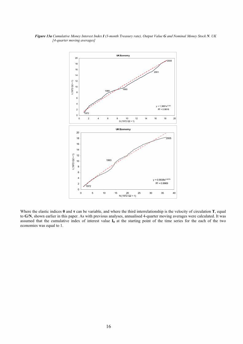
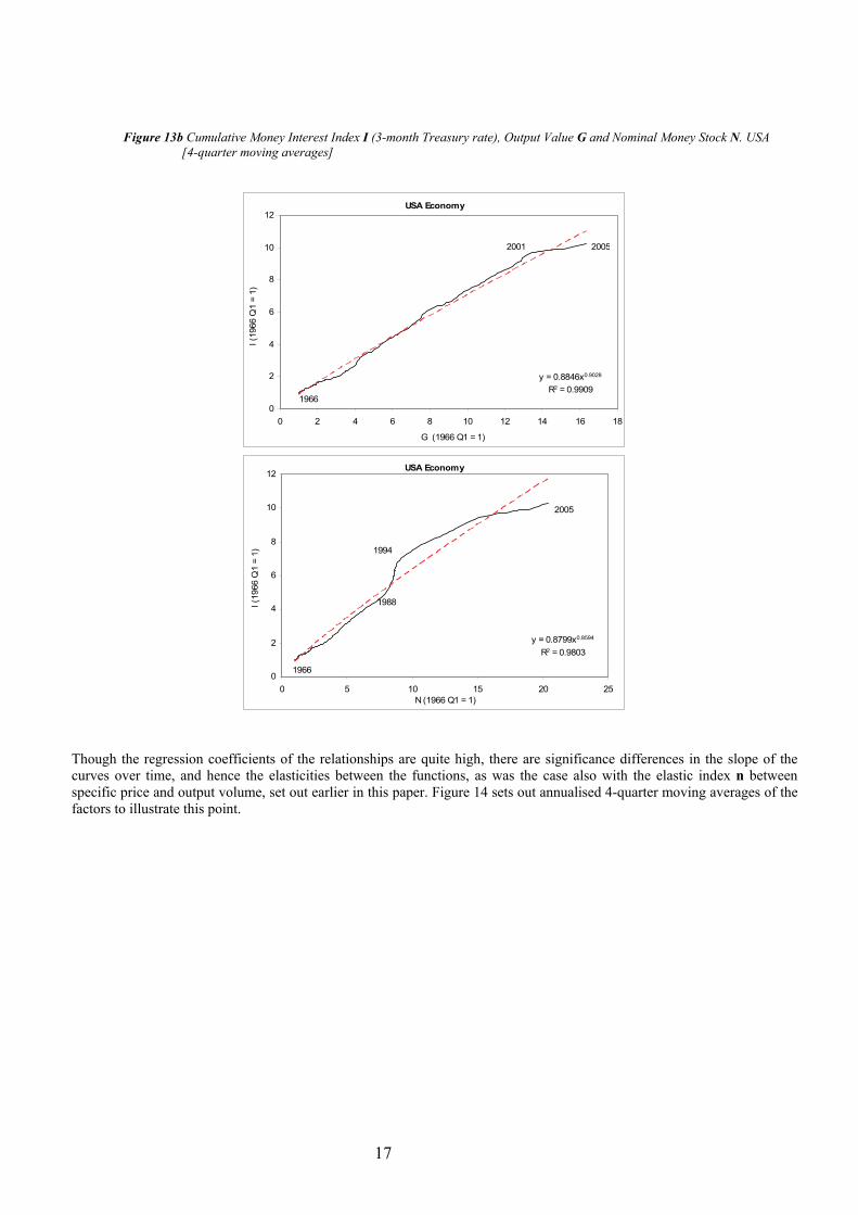
where I0 represents a convenient starting point. Thence, for example, for adjacent points 1 and 2 in time: I2 = I1(1+i2), and (I2 -I1) = i2I1, where i2 is the interest rate applying in the specified year. Thus in general we could express the incremental rate of change of the index I as dI/I, being equal to the variable interest rate i at any point in time. Although money balances N exist primarily to facilitate flow of value within an economy, it is not unreasonable to accept that when they reside in a deposit account they will accumulate interest, as would money lent to borrowers accumulate chargeable interest. Such interest, when payable or chargeable, is included in the total of money balances. Thus there might be a relationship between our cumulative interest index value I and both output value G and money balances N, depending upon the use in economic output value, and time spent on balance (which is a function of the velocity of circulation T). It will be appreciated of course that with high inflation the index I is likely to rise significantly with larger interest rates implied. Likewise the number of money instruments N tends to rise as the currency is depreciated, and output value rises as prices and inflation escalate. Figures 13a and 13b set out relationships between the cumulative interest index I (calculated from quarterly values of 3-month treasury rates), output value G (equal to price level P x output volume V), and nominal money balances N, with trend lines calculated according to the equation:

τθ

⎟⎟⎠

⎞⎜⎜⎝

⎛=⎟⎟

⎠

⎞⎜⎜⎝

⎛=⎟⎟

⎠

⎞⎜⎜⎝

⎛

1

2

1

2

1

2

NN

GG

II

or N

dNGdG

IdI τθ == (20)

16

Figure 13a Cumulative Money Interest Index I (3-month Treasury rate), Output Value G and Nominal Money Stock N. UK [4-quarter moving averages]

UK Economy

y = 1.3881x0.903

R2 = 0.9816

0

2

4

6

8

10

12

14

16

18

20

0 2 4 6 8 10 12 14 16 18 20G (1972 Q2 = 1)

I (19

72 Q

2 =

1)

1972

2005

19931989

2001

UK Economy

y = 0.9038x0.8578

R2 = 0.9969

0

2

4

6

8

10

12

14

16

18

20

0 5 10 15 20 25 30 35 40N (1972 Q2 = 1)

I (19

72 Q

2 =

1)

2005

1993

1972

Where the elastic indices θ and τ can be variable, and where the third interrelationship is the velocity of circulation T, equal to G/N, shown earlier in this paper. As with previous analyses, annualised 4-quarter moving averages were calculated. It was assumed that the cumulative index of interest value I0 at the starting point of the time series for the each of the two economies was equal to 1.

17

Figure 13b Cumulative Money Interest Index I (3-month Treasury rate), Output Value G and Nominal Money Stock N. USA [4-quarter moving averages]

USA Economy

y = 0.8846x0.9028

R2 = 0.9909

0

2

4

6

8

10

12

0 2 4 6 8 10 12 14 16 18

G (1966 Q1 = 1)

I (19

66 Q

1 =

1)

1966

20052001

USA Economy

y = 0.8799x0.8594

R2 = 0.9803

0

2

4

6

8

10

12

0 5 10 15 20 25N (1966 Q1 = 1)

I (19

66 Q

1 =

1)

2005

1966

1988

1994

Though the regression coefficients of the relationships are quite high, there are significance differences in the slope of the curves over time, and hence the elasticities between the functions, as was the case also with the elastic index n between specific price and output volume, set out earlier in this paper. Figure 14 sets out annualised 4-quarter moving averages of the factors to illustrate this point.

18

Figure 14 Annualised changes (4-quarter moving averages) in output value G, nominal money stock N, and the negative of interest rates (3-month Treasury rate).

UK Economy

-20

-10

0

10

20

30

1972 Q2 1976 Q2 1980 Q2 1984 Q2 1988 Q2 1992 Q2 1996 Q2 2000 Q2 2004 Q2

% p

er a

nnum

dG/G

Negative Treasury 3-month rate

dN/N

USA Economy

-20

-16

-12

-8

-4

0

4

8

12

16

20

1966q1 1970q1 1974q1 1978q1 1982q1 1986q1 1990q1 1994q1 1998q1 2002q1

% p

er a

nnum

dG/GdN/NNegative Treasury 3-montn rate

It is generally accepted among economists that the demand for money is positively related to income and output, but negatively related to interest rates. Proceeding further, the standard textbook representation of demand for money is by reference to a curve of liquidity preference, a concept pioneered by Keynes (1936) in his book The General Theory of Employment, Interest and Money. Liquidity preference is effectively a curve of utility of money turned upside down, as in figure 15. At this point it should be stated that we are not arguing in favour of either a Keynesian or Monetarist approach to economics, and whether management of the money supply or adjustments in fiscal spending provide the means to keep an economy in balance. We are, however, arguing that the thermodynamic analysis set out so far indicates that economies appear to operate with a polytropic relationship between specific price, output volume and velocity of circulation, with interrelating elasticities, albeit that these do change. We are also arguing that there is a relationship between the concepts of utility and entropy, and therefore that the utility of money can be represented in terms of entropic value. A number of researchers have highlighted similarities between economic utility theory and thermodynamic concepts, in particular entropy. Candeal, Miguel et al (2001) describe a similarity between the utility representation problem in utility theory and the entropy representation problem related to the second Law of Thermodynamics. Sousa and Domingos (2005, 2006) describe a number of aspects of both utility theory and thermodynamics. Smith & Foley (2002, 2004) highlight similarities between utility and entropy.

19

Figure 15 Liquidity Preference and Utility of Money

Thus the inference of the analysis is that interest rates are negatively related to changes in money entropy value. The higher the level of money entropy change, and the higher price inflation, the more negative interest rates have to be to counteract the forces in the economy. Interest is therefore a form of value flow constraint and negative entropy. To connect interest rates to both output value G and entropy s the following relationship is proposed: “In an economic system, the difference between the rate of change in output value flow G and the rate of change in the Index of Money Interest I is a function of residual changes in money entropy generated or consumed.” This is expressed as:

⎥⎦⎤

⎢⎣⎡ −=

IdI

GdGfdsmoney (21)

where dI/I is the short-term interest rate i at any point in time. If further we assume that the function f of equation (21) is equal to unity, and the elastic factor θ at equation (20) is absorbed into the incremental entropy change ds, then equation (21) becomes:

I

dIGdGdsmoney −= (22)

In this equation the rate of change in the cumulative interest index I is a function of the rate of change in output value G, but is negatively related to change in money entropy. Further, by substituting in the general money equation (3):

TdT

NdN

VdV

PdP

GdG

+=+=

We have:

moneydsTdT

IdI

NdN

+−= (23)

It will be noted that this equation also has the same format as in our initial money hypothesis set out at equation (17). Thus the rate of change in money supply is equated to interest rates less the rate of change in the velocity of circulation plus the residual entropy change. By deducting the rate of change in output volume dV/V from both sides of equation (22) we can also write:

Demand

Interest charged

Demand

Liquidity Preference Utility of Money

Utility

20

rev

money VdVds

IdI

PdP

−=− (24)

Now from equation (22), by substituting in equation (13) for the money entropy change:

rev

money TdT

nkds ⎟

⎠⎞

⎜⎝⎛

−+=

11ω

And assuming nominal money value k=1, we have:

rev

money TdT

nds

IdI

GdG

⎟⎠⎞

⎜⎝⎛

−+==−

11ω or ( ) nTIAG −

+= 11

1ω

(25)

From equation (25) and by substitution of the general money equation (3) and/or the elastic relationship:

( )VdVn

TdT

−= 1

The following identities can be derived:

revV

dVTdT

IdI

GdG

+=− ω or ( )ωTIVAG 2= (26)

( )revV

dVnI

dIGdG 1+−=− ωω or ( ) 1

3+−= nVIAG ωω

(27)

revTdT

IdI

PdP ω=− or ( )ωTIAP 4= (28)

( )revT

dTVdV

IdI

NdN 1−+=− ω or ( ) 1

5−= ωTIVAN (29)

revT

dTn

nI

dIN

dN⎟⎠⎞

⎜⎝⎛

−+=−

1ω or ( ) n

nTIAN −

+= 16ω

(30)

( )revV

dVnnI

dIN

dN+−=− ωω or ( ) nnVIAN +−= ωω

7 (31)

Where the factors A1 to A7 are constants of integration. Equations (25) – (31) represent seven forms of the same identity. Figures 16 – 18 set out charts of the relationships, based on annualised 4-quarter moving average data of the UK and USA economies. For all the charts, it was assumed that the value capacity coefficient ω for both UK and USA economies was 0.75. Because of the ‘noise’ inherent in the data, technical changes in the value capacity coefficient ω (and hence changes in long-run velocity of circulation), the variability of the elastic index n, and changes in the impact of interest rates on an economy (see equation (20) and figures 13a and 13b) it is inevitable that there will significant deviations between values on either side of each equation. For example, the correlation coefficient for the UK economy of dG/G-i versus Δs is of the order R2 = 0.53, quite low. Thus much work is still required to improve and refine the relationships, perhaps by considering lag/lead relationships, and modelling some of the technical changes. The initial result is, nevertheless, quite interesting as each of the results appears to follow quite closely the ebb and flow of the money entropy change.

21

Figure 16 Output value G, interest rates and entropy change [4-quarter moving averages]

UK Economy

-15

-10

-5

0

5

10

15

20

1972 Q2 1976 Q2 1980 Q2 1984 Q2 1988 Q2 1992 Q2 1996 Q2 2000 Q2 2004 Q2% p

er a

nnum

Δs (ω=0.75)dG/G-i(ω-ωn+1)dV/V

USA Economy

-10

-5

0

5

10

15

1966q1 1970q1 1974q1 1978q1 1982q1 1986q1 1990q1 1994q1 1998q1 2002q1

% p

er a

nnum

Δs (ω=0.75)dG/G-i(ω-ωn+1)dV/V

22

Figure 17 Interest rates, price and velocity of circulation [4-quarter moving averages]

UK Economy

0

5

10

15

20

25

1972 Q2 1976 Q2 1980 Q2 1984 Q2 1988 Q2 1992 Q2 1996 Q2 2000 Q2 2004 Q2

% p

er a

nnum

.

Interest rate

dP/P - ωdT/T

USA Economy

-4

0

4

8

12

16

1966q1 1970q1 1974q1 1978q1 1982q1 1986q1 1990q1 1994q1 1998q1 2002q1

% p

er a

nnum

dP/P - ωdT/T

Interest rate

23

Figure 18 Money Balances N, interest rates, entropy and velocity of circulation [4-quarter moving averages]

UK Economy

-10

-5

0

5

10

15

1972 Q2 1976 Q2 1980 Q2 1984 Q2 1988 Q2 1992 Q2 1996 Q2 2000 Q2 2004 Q2

% p

er a

nnum

dN/N-iΔs -dT/T(ω-ωn+n)dV/V

USA Economy

-8

-6

-4

-2

0

2

4

6

8

10

12

1966q1 1970q1 1974q1 1978q1 1982q1 1986q1 1990q1 1994q1 1998q1 2002q1

% p

er a

nnum

dN/N-i

Δs -dT/T

(ω-ωn+n)dV/V

From all the previous analysis and discussion, it will be appreciated that economic entropy change, positive or negative, represents a measure of whether an economy is likely to expand or contract. Thus knowing the conditions that define the direction is important. It will be noted that the entropy change set out at equations (25) and (27) has two parts: a factor in the brackets called the entropic index, and either a change in velocity of circulation dT/T or a volume change dV/V. The factors are different for velocity and volume, though the solution for zero money entropy change is still the same n=γ= (ω+1)/ω.

revmoney T

dTn

ds ⎟⎠⎞

⎜⎝⎛

−+=

11ω

( )rev

money VdVnds 1+−= ωω (32)

The two equations are linked by the elastic relationship:

( )VdVn

TdT

−= 1

Thence, for zero money entropy change n=γ= (ω+1)/ω and we arrive as before at equation (15):

revV

dVTdT

⎟⎠⎞

⎜⎝⎛ −=ω

Figure 10 earlier in this paper illustrates the link between money entropy change and rates of change in output volume and velocity of circulation.

24

It can be seen from equations (32) that the condition for positive money entropy change ds is: Factor and multiplicand at equations (32) are either ‘both positive’, or ‘both negative’. And the condition for negative money entropy change -ds is: Factor and multiplicand) must be opposite in sign i.e. factor positive and multiplicand negative, and vice versa. Figure 19 sets out the loci of the entropic indices at equation (32) for varying values of elastic index n and value capacity coefficient ω. Figure 19 Loci of Entropic Indices

-2

-1

0

1

2

0.0 0.5 1.0 1.5

Entro

pic

Inde

x

1.752.002.503.00

Value Capacity

Coefficientω

n increasing

Elastic Index n

⎟⎠⎞

⎜⎝⎛

−+

n11ωEntropic Index wrt Velocity of Circulation

-2

-1

0

1

2

0.0 0.5 1.0 1.5

Entro

pic

Inde

x

1.752.002.503.00

Value Capacity

Coefficientω

Elastic Index n n increasing

( )1+− nωωEntropic Index wrt Volume

25

3. Summary and Conclusion This paper develops further a monetary model of the economy, based on thermodynamic principles, first set out in a paper published in 2007 [Bryant (2007)]. The model is similar in construction to the well-known quantity theory of money, though it has some important differences. Analysis of quarterly economic data of the UK and USA economies was used to provide empirical evidence to back up the theory. By constructing a specific price PN, equal to the GDP deflator divided by money supply (M4 and M3 definitions), and the inverse the specific money NP, equal to money supply divided by the GDP deflator, it was shown that, in the periods covered, both the UK and USA economies appeared to operate on a polytropic basis, with an elastic index n linking specific price PN and output volume V, with a significant level of regression. Similar links were also established between specific price PN and output volume V to the velocity of circulation T. An analysis was set out illustrating the development of the elastic index n for the UK and USA economies. Significant changes in the elastic index n occurred at points where growth in output volume was low or negative. An equation was developed to link incremental money entropy ds with the rate of change of velocity of circulation dT/T and output volume dV/V, and the elastic index n; and illustrated by data of the UK and USA economies. From this analysis further links were derived between money entropy and interest rates, culminating in a set of formal identities linking the rate of change in output value with interest rates and incremental money entropy, further linked by the general money equation PV=NkT, to changes in money supply and the velocity of circulation. These relationships were illustrated by reference to data of the UK and USA economies. The paper points to the need for further work: first to analyse data of other economies to set alongside that of the UK and USA, second to develop better estimates of the value capacity coefficient ω and its relationship to the velocity of circulation T, and third to assess the effects of factors outside money affecting incremental money entropy change.

References

Bryant, J. (2007) ‘A Thermodynamic theory of economics’, Int. J. Exergy, Vol 4, No. 3, pp. 307-337. Candeal, J.C. De Migule, J.R. Indurain, E. Mehta, G. B. (2001) ‘Utility and entropy’, Economic Theory, Springer-Verlag, 17, pp.233-238. Georgescu-Roegen, N. (1971) ‘The entropy law and the economic process’, Harvard University Press, Cambridge, MA. Harrison, S et al. (2007) ‘Interpreting movements in broad money’, Bank of England Quarterly Bulletin, 2007 Q3. Lisman, J. H. C. (1949) ‘Econometrics statistics and thermodynamics’. Netherlands Postal and Telecommunications Services. The Hague, Holland Ch IV Keynes, J.M. (1936), 'The general theory of employment, interest and money' London: Macmillan (reprinted 2007). Pikler, A. G. (1954) ‘Optimum allocation in econometrics and physics’, Weltwirtschaftliches Archiv. Samuelson, P.A. (1970) ‘Maximum principles in analytical economics’, Nobel Memorial Lecture, Massachusetts Institute of Technology, Cambridge, MA. Smith, E. Foley, D. K. (2002) ‘Is utility theory so different from thermodynamics?’, Santa Fe Institute. Smith, E. Foley, D. K. (2004) ‘Classical thermodynamics and general equilibrium theory’, Santa Fe Institute. Soddy, F. (1934) ‘The role of money’, Routledge, London. Sousa, T. Domingos, T. (2005) 'Is neoclassical microeconomics formally valid? An approach based on an analogy with

equilibrium thermodynamics', Ecological Economics, in press. Sousa, T. Domingos, T. (2006) 'Equilibrium econophysics: A unified formalism for neoclassical economics and equilibrium

thermodynamics' Physica A, 371 (2006) pp. 492-512.

26

Appendix I Derivation of Entropy change for a Polytropic Process For a polytropic relationship of the form:

CVP nN =

The work done ΔW from increasing/decreasing output from level (1) to level (2) is given by:

dVVCdVPW nN∫ ∫==Δ

2

1

2

1

Thence by integration and substituting PNVn=C we get:

⎟⎠⎞

⎜⎝⎛

−−

=⎥⎦

⎤⎢⎣

⎡−

=Δ−

nVPVP

nCVW NN

n

111122

2

1

1

And by further substitution of the ideal equation PNV=kT:

( )121TT

nkW −⎟

⎠⎞

⎜⎝⎛−

=Δ

This increase in work level is handled by an increase in the internal value ΔU of the money instruments proportional to the change in the velocity of circulation T, and depending upon the lifetime ω of the money instrument: Thus: ( )12 TTkU −=Δ ω

From the First Law of Thermodynamics we have:

WUQ Δ+Δ=Δ Where ΔQ is the outside value entering or leaving, not represented by productive content or represented by a change in the velocity of circulation of the money instruments, such as a change in utility or inflation caused by scarcity or abundance. Thus by substituting back we have:

( ) ( )1212 1TT

nkTTkQ −⎟

⎠⎞

⎜⎝⎛−

+−=Δ ω

( )1211 TT

nk −⎟

⎠⎞

⎜⎝⎛

−+= ω

Or in differential form:

dTn

kdQ ⎟⎠⎞

⎜⎝⎛

−+=

11ω

From the Second law of Thermodynamics an expression for the entropy change is given by:

revTdQds =

Thence by further substitution, the incremental change in entropy is given by:

revT

dTn

kds ⎟⎠⎞

⎜⎝⎛

−+=

11ω