A Thermo-elastic Annular Plate Model for the Modeling of BrakeSystems∗

Jose Luis Reyes Perez⋄, Andreas Heckmann⋄ and Ingo Kaiser⋄⋄German Aerospace Center (DLR), Institute of Robotics and Mechatronics

Oberpfaffenhofen, 82234 Wessling, Germany

Abstract

The friction forces generated during braking betweenbrake pads and discs produce high thermal gradientson the rubbing surfaces. These thermal gradients maycause braking problems such as brake fade, prematurewear or hot spotting and the associated hot judder phe-nomenon in the frequency range below 100 Hz.

Further consequences are comfort reductions, adefective braking process, inhomogeneous wear, cut-backs of the brake performance and even damage ofbrake components.

The present paper proposes a modeling conceptthat is targeted on this field of application and in-troduces the new Modelica class ThermoelasticPlate,which is implemented in the DLR FlexibleBodies li-brary.

Keywords: Disc brake, Modal multifield ap-proach, Thermoelasticity

1 Introduction

Friction braking is necessarily related to high thermalloads which lead to high temperatures at the surface ofbrake discs and to large thermal gradients as well. Thefriction forces in turn depend on temperature, on loadand sliding speed [1] so that the braking performanceand the related wear phenomena are known to be ruledby a complex interrelationship.

In addition, the thermal loads can initiate the on-set of unevenly distributed hot spots or bands and ther-mally deformed brake discs [2], [3]. Since the brakepads then slide upon a non-smooth surface while thebrake disc rotates, the brake system vibrates, noise isgenerated and undesirable wear occurs.

Due to the conduction of heat to other componentssuch as the caliper, the bearing or the brake fluid fur-

∗Updated and revised version of the paper published at the 8thInternational Modelica Conference, March 20-22, 2011, Dresden.

ther performance reducing or even dangerous effectssuch as brake fluid boiling and vaporization have beenreported by several authors, see e.g. [4].

Besides experimental studies the finite elementmethod (FEM) [5], [6], [7] [8] or analytical techniques[9] [10] are utilized to analyze the thermal and thermo-elastic behavior of brakes in literature.

Both methods have advantages and provide valu-able results, but both methods are not well suited, ifcomplex scenarios such as the interaction of brakeswith suspensions or vehicle control systems are in-vestigated and a system dynamical point of view isadopted.

To this purpose the present paper proposes a novelmodel of a moderately simplified brake disc. Depend-ing on the user input the thermo-elastic behavior ofbrake discs is described with approximately 100 up to1000 degrees of freedom.

The thermal field of the disc is discretized inthree dimensions and the associated states are speci-fied likewise in Lagrangian or in Eulerian representa-tion. An annular Kirchhoff plate is adapted to evaluatethe deformations according to the uncoupled thermo-elastic theory [11, Ch. 2] presuming that the mechani-cal terms in the heat conduction equations are negligi-ble.

In circumferential direction the disc is assumedto be rotational symmetric, in axial direction differ-ent layers with different heat capacity and conduc-tion properties and multiple surfaces, where coolingby convection occurs, may be defined.

In order to implement this concept the Modelicaclass ThermoelasticPlate has been introduced into thecommercial DLR FlexibleBodies library. This paperpresents the underlying theory on thermal and thermo-elastic fields, explains the user interface of the Ther-moelasticPlate class and gives a simulation example.The final section gives an outlook to further efforts inresearch and modeling of friction brakes and its vali-dation, which is supposed to be initiated by the novel

modeling approach.

2 Thermal Field

2.1 Weak Field Equations

In order to describe the thermal behaviour of thebrake disc the weak equations for the temperature fieldϑ(c, t) as functions of the spatial position in cylindri-cal coordinates c = (r, φ, z)T and time t are deducedfrom the principle of virtual temperature, see e.g. [12,(7.7)] or [13, (1.3.33)]:

∫V

[−(∇δϑ)Tq+ρc ϑδϑ] dV + . . .

. . .+∫B

qTBnBδϑ dB = 0 ,

(1)

where ρ denotes the density, c the specific heat capac-ity, dB the boundary element and nB the outer unitnormal vector. q symbolizes the heat flux accordingto Fourier’s law of heat conduction depending on thetemperature gradient ∇ϑ and the thermal conductivitymatrix � [11, (1.12.16)]:

q =−�∇ϑ (2)

The boundary heat flux qB may be given explicitlyor, if convection occurs, may be specified by the filmcoefficient h f and the bulk temperature ϑ∞ of the fluid[11, Sec. 5.6]:

qTBnB =−qB−h f (ϑB−ϑ∞) . (3)

2.2 Modal Approach

The discretization of the scalar temperature is per-formed using the Ritz approximation that allows toseparate the thermal field description by a finite-dimensional linear combination of two parts, the firstone considers thermal modes and is spatial depen-dent, i.e. ΦΦΦϑ = ΦΦΦϑ(c) and the second one repre-sent the modal amplitudes and is time dependent, i.e.zϑ = zϑ(t):

ϑ(c, t) =ΦΦΦϑ(c)zϑ(t) (4)

The spatial mode functions are formulated usingthe separation approach of Bernoulli for the spatial co-ordinates as well, so that (4) may be rewritten as fol-

Figure 1: Example set of B-splines to discretize thethermal field in radial and axial direction.

lows:

n

∑i=1

Φϑi(c)zϑi(t) =n

∑i=1

Ri(r) Ψi(φ) Zi(z) zϑi(t) =

=lm

∑l=1

km

∑k=0

mm

∑m=1

Rl(r) ⋅ cos(kφ) ⋅Zm(z) ⋅ zϑi(t)+

+lm

∑l=1

km

∑k=1

mm

∑m=1

Rl(r) ⋅ sin(kφ) ⋅Zm(z) ⋅ zϑi(t) ,

with i = 1,2, . . . ,n , n = (lmmm)(2km +1) .

(5)

According to Walter Ritz [14], the trial functionshave to be linearly independent and components of acomplete system, so that the number of i may be in-creased as needed in order to improve the approxima-tion. For Rl(r) and Zm(z) B-splines [15] as shown inFig. 1 have been chosen as trial functions in radial andaxial direction, respectively.

The harmonic waves (or Fourier series expan-sion) Ψi(φ) are appropriate in circumferential direc-tion, since

∙ they allow to represent cyclic properties, i.e.Ψi(φ) = Ψi(φ+2π),

∙ they are simple to integrate from 0 to 2π,

∙ their orthogonality leads to block-diagonal sys-tem matrices, i.e. the entire system of equationsis split up into decoupled sub-systems,

∙ they will later on be exploited to provide a Eule-rian description of the thermo-elastic plate.

2.3 Discretized Field Equations

If (5) is inserted into (1), the volume integrals can beseparated from the terms that dependent on time. As a

result, the linear thermal field equation is obtained:

Cϑϑzϑ +(Kϑϑ +KϑR)zϑ =QϑN qB +QϑR ϑ∞ , (6)

where the volume integrals are defined, inter alia usingthe abbreviationBϑ :=∇ΦΦΦϑ, as follows [16, Tab. 2.5]:

the heat capacity matrix: Cϑϑ :=∫

Vρc ΦΦΦT

ϑΦΦΦϑ dV

the conductivity matrix: Kϑϑ :=∫

VBT

ϑ�Bϑ dV

the Robin load matrix: KϑR :=∫

Bh f ΦΦΦT

ϑΦΦΦϑ dB

the Robin load vector: QϑR :=∫

Bh f ΦΦΦT

ϑdB

the Neumann load vector: QϑN :=∫

BΦΦΦT

ϑdB

These volume integrals may therefore be evalu-ated in advance to the simulation or time integration,respectively.

Note, that neither (6) nor (1) comprehend termsthat express the thermodynamics of deformations, sothe so-called thermo-elastic damping phenomenon isdisregarded [11, Ch. 2]. This approach is commonlyknown as uncoupled thermo-elastic theory, which nev-ertheless covers heat energy dissipation of mechanicalprocesses. Indeed, e.g. friction initiates an associatedheat flux qB and therefore enters (6) as external loadQϑNqB which corresponds to Neumann boundary con-ditions in the partial differential equation related to (6).

2.4 The Eulerian Description

Figure 2: Coordinate transformation with angle χ, thatleads from the Lagrangian to the Eulerian description.

It is now considered that the brake disc performsa rotation around its central axis specified by the angleχ(t). So far the temperature field is described in theso-called Lagrangian point of view [17, Sec. I.3], i.e.the reference frame follows the rotation as it is shownfor the coordinate system named B in Fig. 2.

However for the specific use case treated here itmay make sense to resolve the temperature field of the

disc in frame A in Fig. 2. In other words, the observerdoes not rotate with the disc but looks on the plate fromthe outside, from a point in rest concerning the rotationwith angle χ(t).

This concept is the so-called Eulerian description[17, Sec. I.4] and is widely used in fluid dynamics,where the motion state of the fluid at a fixed point inspace is presented. Due to the rotational symmetryproperties of the brake disc the Eulerian descriptioncan here be formulated in an elegant and convenientway.

For theoretical derivation the coordinate transfor-mation

φ = θ−χ (7)

is defined, where θ specifies the angular position of anobserved point on the brake disc resolved with respectto the Eulerian reference system A in Fig. 2.

Furthermore it is assumed that for every trial func-tion in (5) that employs a sin(kφ)-term an associatedtrial function is present where the sinus- is replaced bythe cosinus-function only, but Rl(r), Zm(z) and k areidentical, so that mode shape couples c1 and c2 exist:

c1(r,φ,z) = Rl(r) ⋅Zm(z) ⋅ sin(kφ) ,

c2(r,φ,z) = Rl(r) ⋅Zm(z) ⋅ cos(kφ) .(8)

If the following identities

sin(kφ) = sin(kθ)cos(kχ)− cos(kθ)sin(kχ) ,

cos(kφ) = cos(kθ)cos(kχ)+ sin(kθ)sin(kχ)(9)

are inserted into (8), an associated mode couplec1(r,θ,z) and c2(r,θ,z) defined with respect to frameA appears:

c1 = RlZm sin(kθ)︸ ︷︷ ︸:=c1(r,θ,z)

cos(kχ)−

−RlZm cos(kθ)︸ ︷︷ ︸:=c2(r,θ,z)

sin(kχ) ,

c2 = c1(r,θ,z)sin(kχ)+ c2(r,θ,z)cos(kχ) .

(10)

As a result of suitable transformations it may also bewritten:

c1(r,θ,z) = c2 sin(kχ)+ c1 cos(kχ) ,

c2(r,θ,z) = c2 cos(kχ)− c1 sin(kχ) .(11)

The mode functions c1(r,θ,z) and c2(r,θ,z) aredefined in the Eulerian reference system A and arelinear combinations of the mode functions c1(r,φ,z)and c2(r,φ,z) described in the Lagrangian frame B ,whereas the combination depends on χ(t).

This information can be exploited in order to de-fine a transformation: a thermal field resolved in theLagrangian frame can be transformed to be resolved inthe Eulerian frame and vice versa. Of course the phys-ical temperature field itself does not change, but itsresolution does so that the numerical values describingthe field will be different in frame A or B , respectively.

In practice the transformation is formulated interms of the modal amplitudes zϑi(t) which are thethermal states in (6):

zϑi1(t) = sin(kχ(t))zϑi2(t)+ cos(kχ(t))zϑi1(t) ,

zϑi2(t) = cos(kχ(t))zϑi2(t)− sin(kχ(t))zϑi1(t) .(12)

Again, the new modal amplitudes in the Eulerianframe zϑi(t) are expressed as a linear combination ofmodal amplitudes in the Lagrangian frame zϑi(t) andit is just a matter of convenience and practicability inwhich coordinates the thermal field equations are ac-tually evaluated.

One particularity has been ignored so far. Fortrial functions with k = 0 no mode couple with c1 andc2 according to (8) exists, since no associated sinus-function is introduced in (5). As a consequence thetransformation (12) is not defined for such modes.However, trial functions with k = 0 represent rota-tional symmetric fields since the dependency on φ iseliminated in (5) due to the term cos(kφ). As a conse-quence mode shapes with k = 0 are invariant with re-spect to rotations with angle χ or in other words: Themodal coordinates zϑi(t) related to k = 0 are identicalin the Eulerian and the Lagrangian description and notransformation is needed.

3 Mechanical Field

The present paper is focused on the thermo-elastic in-terrelation that rules the behavior of brake discs in thelow frequency range. Note that there is a complemen-tary paper presented on this Modelica User Confer-ence which is dedicated to higher frequencies in orderto cope e.g. with brake squeal phenomena [18]. How-ever here, it is supposed that the excitation is muchlower than the lowest natural frequency of the brakedisc. In particular the following assumption are made:

∙ The structural deformations of the brake disc aredominated by its elasticity or thermo-elasticity,respectively. Inertia effects are out of focus andin particular the influence of the brake disc ro-tation on the deformations are negligible. Thisstatement is related to the so-called Duhamel’s

assumption which argues on the different time-scales with which changes in the temperature ordeformation field usually proceed, cp. [11, Sec.2.5].

∙ A literature review on the characteristics ofthermo-elastic brake disc deformation give rea-son to the assumption that plate bending in somecases even plate buckling is the governing defor-mation mechanism, see [9], [2], [6]. For example:all experimental studies describe e.g. hot spots tobe located alternatively on the two disc surfacesin anti-symmetrical configuration, so that the cir-cumference is deformed similar to a sinuous line.Therefore the deformation field of the brake dischere is represented as an annular Kirchhoff plate.

Note that the description of the annular plate is lim-ited to be linear in this initial implementation, so thatplate buckling phenomena are not covered, see [19],[20, Ch. 1]. An extended formulation to consider ther-mal buckling is a field of active research at the DLR.

3.1 Thermo-elastic Coupling

In [16, Sec. 2.2] the material constitution based ona thermodynamical potential is harnessed to formu-late the interrelation of the thermal and the mechanicalfield. This approach is not suited here, since the influ-ence of a 3-dimensional thermal on a 2-dimensionaldisplacement field is to describe.

Instead the so-called body-force analogy is em-ployed, i.e. the thermo-elastic problem is transferedinto an isothermal problem with equivalent distributedbody forces �ϑ [11, §3.3], whose non-zeros compo-nents in radial and tangential direction read:

�ϑr = �ϑφ =−1+ν

1−ν2 Eα ϑ , (13)

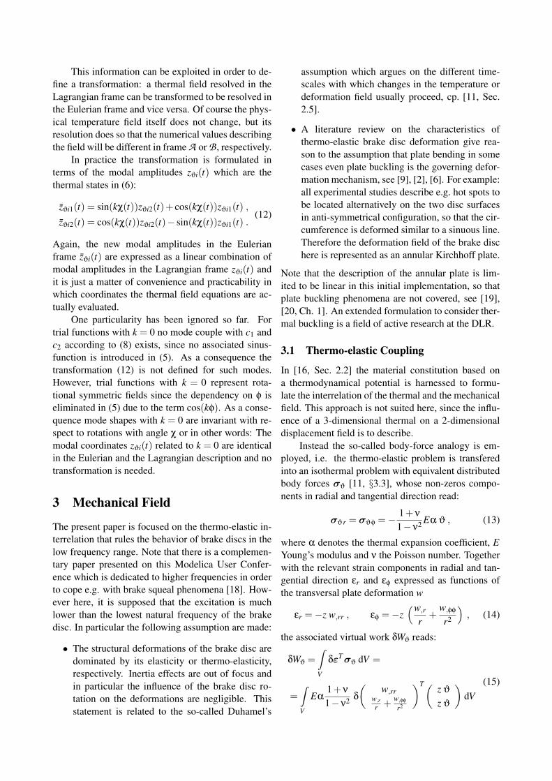
where α denotes the thermal expansion coefficient, EYoung’s modulus and ν the Poisson number. Togetherwith the relevant strain components in radial and tan-gential direction εr and εφ expressed as functions ofthe transversal plate deformation w

εr =−z w,rr , εφ =−z(w,r

r+

w,φφ

r2

), (14)

the associated virtual work δWϑ reads:

δWϑ =∫V

δ"T�ϑ dV =

=∫V

Eα1+ν

1−ν2 δ

(w,rr

w,rr +

w,φφ

r2

)T( z ϑ

z ϑ

)dV

(15)

3.2 Weak Field Equations

The structural displacements u are evaluated on thebasis of the principle of virtual displacements [12,(4.7)], which states that the virtual work of the internalforces equals the virtual work of the interia and exter-nal forces:∫

V

δ"T� dV +∫V

δ"T�ϑ dV+

+∫V

δuT u ρdV = ∑i

δuTfi ,(16)

where " denotes the strain and � the stress field. fi

represent the applied external forces.

3.3 Modal Approach

Again a Ritz approximation is used to discretize thedeformation field u:

u(c, t) =ΦΦΦu(c)zu(t) (17)

The spatial shape functions in (17) are formulatedas function of cylindrical coordinates, i.e. ΦΦΦu =ΦΦΦu(r,φ,z), w,r and w,φ are partial derivatives with re-spect to r or φ:

n

∑i=1

ΦΦΦuizui =

⎡⎢⎣ −z(cos(φ)w,r− sin(φ)r w,φ)

−z(sin(φ)w,r +cos(φ)

r w,φ)w

⎤⎥⎦ ,w =

lm

∑l=0

km

∑k=0

Rl(r) ⋅ cos(kφ) ⋅ zui(t)+ . . .

. . .+lm

∑l=0

km

∑k=1

Rl(r) ⋅ sin(kφ) ⋅ zui(t) ,

with i = 1,2, . . . ,n , n = (lm +1)(2km +1) .

(18)

The trial functions in (18) correspond to the trialfunctions in (5) except of the fact, that a 2-dimensionalfield is discretized here, while the temperatures dependon all three coordinates.

3.4 Discretized Field Equations

If (18) is inserted into (16) the linear field equation forthe displacements is yielded:

Muuzu+Cuuzu+Kuuzu+Kuϑzϑ =∑i

ΦΦΦTuifi . (19)

The mass matrix Muu in (19) denotes the volume in-tegral

Muu :=∫

V�T

u�u ρdV , (20)

the stiffness matrix Kuu is defined using the lin-ear displacement-strain operator ∇u, the abbreviationBu := ∇uΦΦΦu and the elasticity tensorH:

Kuu :=∫

VBT

uHBu dV . (21)

As usual, the introduction of the damping matrixCuu as an assembly of mass and stiffness terms is jus-tified by empirical considerations [12, Sec. 4.2]. Thethermo-elastic coupling matrix follows from (15):

Kuϑ :=∫V

Eα1+ν

1−ν2 ⋅

⋅(

ΦΦΦu,rr +ΦΦΦu,r

r+

ΦΦΦu,φφ

r2

)T

z ΦΦΦϑ dV

(22)

In addition to the deformations, the motion of thedisc’s reference frame located at the center of grav-ity is considered by the Newton-Euler equations [21,(8.6),(8.21)]:

m ⋅a= ∑fi ,

I!+!×I! = ∑ci×fi +∑pi .(23)

a denotes the translational acceleration of the refer-ence frame, ! its rotational velocity. I symbolizes theinteria tensor, m its mass. fi presents the discrete ex-ternal forces, pi discrete external torques.

4 User Interface

4.1 The Icon Layer

Figure 3: Icon layer of the ThermoelasticPlate class.

The icon layer of ThermoelasticPlate class isshown in Fig. 3. The connector arrays frames top andframes bottom both represent points that slide on the

upper or the lower surface of the plate, respectivelyand therefore are potential connectors to apply brakeforces. The associated heat fluxes generated by fric-tion may be applied to the companion heat port arraysportes top and portes bottom. Each of these arrayscontains as much connectors as are specified by thefirst dimension of the input parameter xsi in the fol-lowing table:

geometrical parametersr i [m] inner radius of the plater a [m] outer radius of the plateth[:] [m] thickness of the platexsi[:,2] [−] points on the disc

Each row of xsi specifies the radial and the angular po-sition of two surface points with respect to the frameA in Fig. 2 parametrized in the interval [0,1]. E.g.xsi[1, :] = {0.5,0.125} defines two surface points inthe middle between the inner and outer radius at 45∘

angular position.In addition to the 3-dimensional multibody frame

connectors, two 1-dimensional rotational flanges areshown in Fig. 3. These two flanges are connected toboth sides of the 3-dimensional rotational joint whichis introduced into the ThermoelasticPlate class at theplate axis by default. The two flanges are conditionallyinstantiated controlled via user parameter and can beutilized to e.g. define constant rotation velocity.

4.2 The Physical Parameters

The thermal field equations (6) are formulated with re-spect to a reference temperature t ref, which may beinterpreted as linearisation point at which all physi-cal material parameters are specified. t ref is as welldefined by user input and displayed in the icon layeras shown in Fig. 3. Since the model also considerscooling by air convection, another input is necessaryto provide information on the bulk temperature t bulk,which is interpreted relative to the reference tempera-ture t ref.

The table below shows the thermal parameters theuser has to provide in order to employ a Thermoelas-ticPlate instance:

thermal parametersrho[:] [kg/m3] mass densitylamdba[:,3] [W/mK] thermal conductivityc [K/kgK] specific heat capacityh fouter [W/m2K] convective heat coeff.h finner [W/m2K] convective heat coeff.al pha [1/K] thermal expansion coeff.

The physical properties are assumed to be homo-geneous in radial and tangential direction, while dif-ferent sections may be defined in axial direction. Thisis why the geometrical input parameter th is definedas a vector. E.g. the values th = {0.003,0.007,0.01}specify three thickness sections from 0 to 3 mm, from3mm to 7 mm and from 7 to 10mm.

As a consequence, the input dimensions of th, rho,lambda and the Young’s modulus E to be introducedbelow are related, since e.g. the density rho[1] is sup-posed to specify the mass density in the first section,i.e. is assigned to the thickness region from 0 to 3 mmfor the given example of th. Each column of the pa-rameter lambda, i.e. lambda[:,i] is also related to thesection from th[i-1] to th[i], while the first elementlambda[1,i] specifies the thermal conductivity in ra-dial, the second element lambda[2,i] in axial and thethird element lambda[3,i] in tangential direction.

By this set-up it is intended to approximately ac-count for a brake disc design as it is shown in Fig. 4.The reduced heat capacity of the center region with thecooling channels may be considered by a reduced massdensity. An appropriate definition of lambda speci-fies heat conduction in the center region only to oc-cur in axial but not in radial or tangential direction.The coefficient h finner quantifies the heat transfer fromthe brake disc to the circulating air at the areas withth[i]=0.003 and th[i]=0.007 in the given example ofth. The input parameter h fouter refers to the convectiveheat transfer at both outer surfaces of the brake disc.

Figure 4: Cooling channels in a brake disc.

The mechanical parameters have to be given asfollows:

mechanical parametersE[:] [N/m2] Youngs’s modulusny [−] Poisson numberdamping [−] natural damping coefficient

The Young’s modulus E as a function of the thick-ness coordinate th is used to evaluate the flexural rigid-

ity of the Kirchhoff plate according to the theory ofmulti-layered plates [22, 3.7] in order to reflect the in-fluence of the cooling channels on the bending behav-ior.

If (19) is given in normal or principal coordinates,see e.g. [23, 6.5], the homogeneous equations of mo-tion will be separated in independent equations of thefollowing typ:

zu,i +2δiωi zu,i +ω2i zu,i = 0 (24)

with the eigenvalue ωi and the natural damping coef-ficient δi. The input parameter damping controls theassembly of the damping matrix Cuu in such a waythat δi equals damping for all normal coordinates. Asa default value damping=1 is specified which corre-sponds to critical damping. This set-up follows the as-sumption that thermoelastic deformations and externalexcitations act in a frequency range much lower thanthe first natural frequency of the plate and inertia ef-fects may be neglected. However, it is up to the userto define alternative damping regimes by giving othervalues for damping.

4.3 The Discretization Set-up

The input parameter vector th implicitly also rules thediscretization of the thermal field in axial direction,which is done by B-spline functions, see Fig. 1. Inthis context, the parameter values of th are interpretedas elements of the so-called knot vector [15]. Depend-ing on the dimension of th, constant, linear, quadraticor cubic B-splines are applied.

The discretization of the thermal field in radial di-rection is specified by the input parameter radialD-iscretization, which directly defines the number ofdegrees of freedom in radial direction. Due to theB-spline concept the order of the trial-functions is as-sociated to the number of degress of freedom, so thatthe following relations hold:

radialDiscretization B-spline type1 constant2 linear3 linear4 linear5 quadratic6 quadratic≥7 cubic

In principle the parameter radialDiscretizationalso counts for the mechanical field with one excep-tion: exclusively cubic B-spline functions are used to

describe the bending deformations with respect to theradius. If necessary to satisfy this basic demand ad-ditional number of degrees of freedom are introducedfor the mechanical field in addition to the input speci-fication of radialDiscretization.

The integer parameter vector angularDiscretiza-tion contains the ordinal numbers of the Fourier termsk from (5) which are to be considered in order to de-scribe the thermal and the mechanical field in circum-ferential direction.

Finally, the user has to choose the boundary con-dition for the displacement field at the inner radius outof two options, namely supported or clamped.

5 Simulation Example

Figure 5: Diagram layer of the brake model.

The example shown in Fig. 5 is a representationof a braking system which illustrates an application ofthe thermo-elastic plate model. The model containsa floating caliper with brake pads sliding along bothsides of the brake disc. A constant rotation velocity of6π rad/s and a constant hydraulic force are specified.An axial run-out of the brake disc is simulated sincethe disc is tilted around its y-axis with 0.005 rad am-plitude and 6 Hz, see the revolute joint in Fig. 5. Aconstant friction coefficient of ν = 0.9 assumed. Thebrake disc is 10 mm thick, 70 mm and 120 mm arespecified as inner radius and outer radius, and its phys-ical parameters correspond to cast iron material.

A second order Fourier expansion is applied todiscretize both fields in circumferential direction, fourlinear B-splines are used for the axial discretization,three linear B-splines for the radial discretization ofthe thermal field.

The disc-pad contact is defined at 9 points at eachside of disc, which are located at −28.8∘ ≤ θ≤ 28.8∘

Figure 6: Diagram layer of the contact submodel.

angular position. The contact is formulated with oneprismatic joint in axial direction for each contact point.frame a in Fig. 6 is supposed to provide the connectionto the brake caliper, frame b is to be connected to oneframe at the surface of the thermoelasticPlate, port bis the associated heat port to define the heat flow intothe brake disc.

In addition the variable port b.T represents thetemperature at the contact point and might be used toformulate e.g. temperature-dependent friction behav-ior in future scenarios. Secondary heat flows e.g. tothe caliper body or thermal contact resistances may beincluded into this configuration as well. Even phenom-ena such as brake fluid boiling [4] may be investigatedby appropriate straight-forward model extensions.

The non-linear spring-damper element attached tothe prismatic joint represents the contact stiffness andis capable to consider the loss of contact or the lift-offof the brake pads, respectively. However this effectis not part of the presented simulation scenario. Thesimplicity of the contact modeling here again demon-strates the advantages of the Eulerian description.

Fig. 7 presents an animation of the simulation sce-nario. The green arrows visualize the friction forces,the color of the plate surface indicates the temperaturedistribution, which in general exposes a maximum atthe trailing edge of the brake pads.

Figure 7: Animation of the brake model.

The exciation by the axial run-out leads to oscil-lations of the normal and tangential forces inverselyphased on the top and the bottom surface of the brakedisc. The influence of this excitation on the thermalfield is presented by the curves in Fig. 8. The de-tailed plot below reveals a antisymmetric pattern of thetemperature distribution at both surfaces of the brakedisc, although the actual temperature differences areindeed small. In addition the general temperature riseis stepped by the rotation frequency of the brake disc.

Another result of the axial run-out is shown inFig. 9, where the bending deformations at the outerradius at θ = 0∘ angular position are plotted as a func-tion of time.

Figure 8: Exemplary temperature results at the top andthe bottom surface, r = 0.102 m, θ = 0∘.

Figure 9: Plot of the plate deformation at the outerradius at θ = 0∘ angular position.

It should be mentioned that these preliminary re-sults still must be validated. Nevertheless the resultscan be interpreted in a physical way and are plausible.

The brake disc model considers 60 thermal and30 mechanical degrees of freedom and 106 cpu-s on acommon laptop are spent to simulate the scenario with40 s simulation time.

6 Conclusions and Outlook

The present paper introduces a new Modelica classcalled ThermoelasticPlate. This model is tailored torepresent the thermal and thermo-elastic behavior ofbrake discs in the lower frequency range. The advan-tages of the Eulerian approach are exploited, so thatthe non-rotating normal and friction forces and the as-sociated heat fluxes may easily be applied.

An example study demonstrates the application ofthe new Modelica class. Although validation of thepresented analysis is still a pendent task, the resultshowever have shown a good agreement with the physi-cal description of this phenomenon giving a solid basisto cope with some of the most common braking prob-lems such as hot spotting. It has been demonstratedthat the approach is open for a wide range of applica-tion scenarios such as temperature-dependent frictionand brake-fluid boiling.

Moreover, the purpose of this project is to in-tegrate the thermo-elastic model into more complexscenarios, such as a complete braking system of atrain (Figure 10 ) which includes brake disc (thermo-elastic model), brake pads, rockers, brake pad hold-ers, calipers, housing, brake piston, etc., in order toanalyze the induced vibrations, due to the thermo-mechanical deformations, into the complete dynamics

Figure 10: Braking mechanism of a train.

of the entire system.

7 Acknowledgements

The authors highly appreciate the partial financial sup-port of Knorr-Bremse Systems for Railway Vehicles inMunich.

References

[1] S.K. Rhee. Friction coefficient of automotivefriction materials − its sensitivity to load, speed,and temperature. SAE Technical paper 740415,1974.

[2] S. Panier, P. Dufrenoy, and D. Weichert. An ex-perimental investigation of hot spots in railwaydisc brakes. Wear, 256:764 – 773, 2004.

[3] T.K. Kao, J.W. Richmond, and A. Douarre.Thermo-mechanical instability in braking andbrake disc thermal judder: an experimental andfinite element study. In Proc. of 2nd Interna-tional Seminar on Automotive Braking, RecentDevelopments and Future Trends, IMechE, pages231–263, Leeds, UK, 1998.

[4] K. Lee. Numerical prediction of brake fluid tem-perature rise during braking and heat soaking.SAE Technical Paper 1999-01-0483, 1999.

[5] A. Rinsdorf. Theoretische und experimentelleUntersuchungen zur Komfortoptimierung vonScheibenbremsen. Hoppner und Gottert, Siegen,1996.

[6] T. Steffen. Untersuchung der Hotspotbil-dung bei Pkw-Bremsscheiben. Number 345 inVDI–Fortschrittsberichte Reihe 12. VDI-Verlag,Dusseldorf, 1998.

[7] T. Tirovic and G.A. Sarwar. Design synthesisof non-symmetrically loaded high-performancedisc brakes, Part 2: finite element modelling.Proc. of the I Mech E Part F: Journal of Rail andRapid Transit, 218:89 – 104, 2004.

[8] P. Dufrenoy. Two-/three-dimensional hybridmodel of the thermomechanical behaviour ofdisc brakes. Proc. of the I Mech E Part F: Jour-nal of Rail and Rapid Transit, 218:17 – 30, 2004.

[9] K. Lee and J.R. Barber. Frictionally excited ther-moelastic instability in automotive disk brakes.Journal of Tribology, 115:607 – 614, 1993.

[10] C. Krempaszky and H. Lippmann. Friction-ally excited thermoelastic instabilities of annularplates under thermal pre-stress. Journal of Tri-bilogy, 127:756–765, 2005.

[11] B.A. Boley and J.H. Weiner. Theory of Ther-mal Stresses. Dover Publications, Mineola, NewYork, 1997.

[12] H.J. Bathe. Finite Element Procedures. PrenticeHall, New Jersey, 1996.

[13] R.W. Lewis, K. Morgan, H.R. Thomas, and K.N.Seetharamua. The Finite Element Method inHeat Transfer Analysis. John Wiley and Sons,Chichester, UK, 1996.

[14] W. Ritz. Uber eine neue Methode zur Losunggewisser Variationsprobleme der mathematis-chen Physik. Journal fur Reine und AngewandteMathematik, 135:1–65, 1908.

[15] Carl de Boor. A practical Guide to Splines.Springer–Verlag, Berlin, 1978.

[16] A. Heckmann. The Modal Multifield Approach inMultibody Dynamics. Number 398 in Fortschritt-Berichte VDI Reihe 20. VDI-Verlag, Dusseldorf,2005. PhD thesis.

[17] J. Salencon. Handbook of Continuum Mechan-ics. Springer-Verlag, Berlin, 2001.

[18] A. Heckmann, S. Hartweg, and I. Kaiser. AnAnnular Plate Model in Arbitrary Lagrangian-Eulerian-Description for the DLR FlexibleBod-ies Library. In 8th International Modelica Con-ference, 2010. submitted for publication.

[19] O. Wallrapp and R. Schwertassek. Representa-tion of geometric stiffening in multibody systemsimulation. International Journal for NumericalMethods in Engineering, 32:1833–1850, 1991.

[20] F. Bloom and D. Coffin. Handbook of ThinPlate Buckling and Postbuckling. Chapman &Hall/CRC, Washington, D.C., 2001.

[21] P.E. Nikravesh. Computer-aided Analysis of Me-chanical Systems. Prentice Hall, EngelwoodCliffs, New Jersey, 1988.

[22] R. Szilard. Theory and Analysis of Plates.Prentice-Hall, Inc., Englewood Cliffs, New Jer-sey, 1974.

[23] L. Meirovitch. Computational methods in struc-tural dynamics. Sijthoff & Noordhoff, Alphenaan den Rijn, Netherlands, 1980.