Arrested Development: Theory and Evidence ofSupply-Side Speculation in the Housing Market∗

Charles G. NathansonHarvard University

cnathans@fas.harvard.edu

Eric ZwickHarvard Universityzwick@fas.harvard.edu

November 2013

JOB MARKET PAPER

Abstract

This paper incorporates speculation into the standard supply-and-demand frame-work used to analyze housing booms and busts. Speculation reverses the common intu-ition that elastic housing supply attenuates housing booms. Housing market frictionsmake land a more attractive speculative investment than housing. As a result, unde-veloped land both facilitates construction and intensifies the speculation that causesbooms and busts in house prices. This insight explains the frequent housing boomsand busts that coincide with high construction activity (e.g. Las Vegas, 2000-2010).These episodes are most likely to occur when a housing market nears but has not yetreached a long-run development constraint. Consistent with the recent U.S. housingexperience, the model predicts higher price volatility in neighborhoods where housingis more easily rented. Land is an asset whose price volatility can increase with its float.

∗We thank John Campbell, Edward Glaeser, David Laibson, and Andrei Shleifer for outstanding adviceand Robin Greenwood, Sam Hanson, Alp Simsek, Amir Sufi, Adi Sunderam, and Jeremy Stein for helpfulcomments. We also thank Harry Lourimore, Joe Restrepo, Hubble Smith, Jon Wardlaw, Anna Wharton, andCoStar employees for enlightening conversations and data. Nathanson thanks the NSF Graduate ResearchFellowship Program, the Bradley Foundation, and the Becker Friedman Institute at the University of Chicagofor financial support.

1

1 Introduction

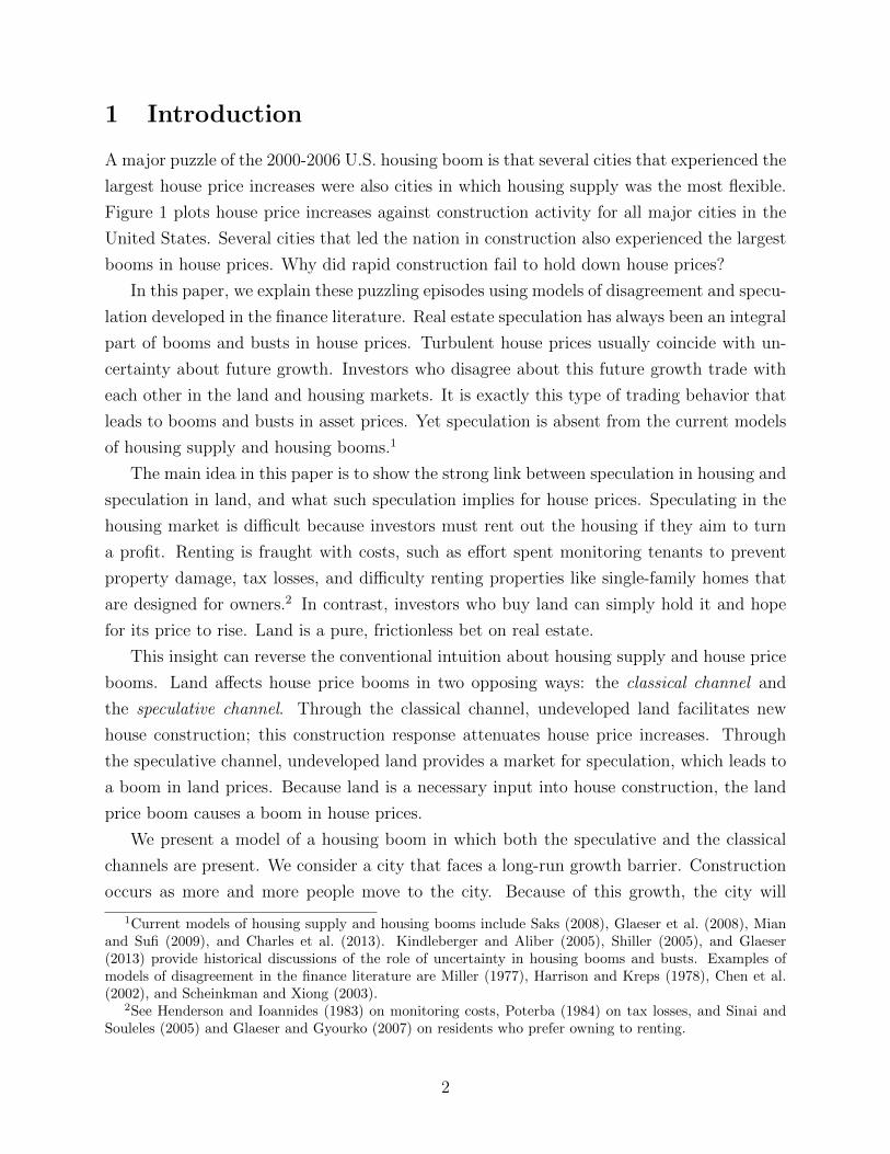
A major puzzle of the 2000-2006 U.S. housing boom is that several cities that experienced the

largest house price increases were also cities in which housing supply was the most flexible.

Figure 1 plots house price increases against construction activity for all major cities in the

United States. Several cities that led the nation in construction also experienced the largest

booms in house prices. Why did rapid construction fail to hold down house prices?

In this paper, we explain these puzzling episodes using models of disagreement and specu-

lation developed in the finance literature. Real estate speculation has always been an integral

part of booms and busts in house prices. Turbulent house prices usually coincide with un-

certainty about future growth. Investors who disagree about this future growth trade with

each other in the land and housing markets. It is exactly this type of trading behavior that

leads to booms and busts in asset prices. Yet speculation is absent from the current models

of housing supply and housing booms.1

The main idea in this paper is to show the strong link between speculation in housing and

speculation in land, and what such speculation implies for house prices. Speculating in the

housing market is difficult because investors must rent out the housing if they aim to turn

a profit. Renting is fraught with costs, such as effort spent monitoring tenants to prevent

property damage, tax losses, and difficulty renting properties like single-family homes that

are designed for owners.2 In contrast, investors who buy land can simply hold it and hope

for its price to rise. Land is a pure, frictionless bet on real estate.

This insight can reverse the conventional intuition about housing supply and house price

booms. Land affects house price booms in two opposing ways: the classical channel and

the speculative channel. Through the classical channel, undeveloped land facilitates new

house construction; this construction response attenuates house price increases. Through

the speculative channel, undeveloped land provides a market for speculation, which leads to

a boom in land prices. Because land is a necessary input into house construction, the land

price boom causes a boom in house prices.

We present a model of a housing boom in which both the speculative and the classical

channels are present. We consider a city that faces a long-run growth barrier. Construction

occurs as more and more people move to the city. Because of this growth, the city will

1Current models of housing supply and housing booms include Saks (2008), Glaeser et al. (2008), Mianand Sufi (2009), and Charles et al. (2013). Kindleberger and Aliber (2005), Shiller (2005), and Glaeser(2013) provide historical discussions of the role of uncertainty in housing booms and busts. Examples ofmodels of disagreement in the finance literature are Miller (1977), Harrison and Kreps (1978), Chen et al.(2002), and Scheinkman and Xiong (2003).

2See Henderson and Ioannides (1983) on monitoring costs, Poterba (1984) on tax losses, and Sinai andSouleles (2005) and Glaeser and Gyourko (2007) on residents who prefer owning to renting.

2

Figure 1: Price Booms and Construction Levels Across Metropolitan Areas

0%

5%

10%

15%A

nn

ua

l H

ou

se

Price

Re

turn

s,

20

00

−2

00

6

0% 1% 2% 3% 4% 5%Annual Housing Stock Growth, 2000−2006

AZ, CA, FL, NV

Notes: The figure includes all metro areas with populations over 500,000 in 2000 for which we have data. Wemeasure each metro area’s housing stock from 2000-2006 using the Census 2000 housing stock estimate andthe 2000-2005 Census housing permit data. We measure each metro area’s 2000 and 2006 house price usingthe FHFA housing price index deflated by the CPI-U. Both housing stock growth and house price returnare reported in log points (1% = 1 log point). The highlighted metro areas are those in Arizona, California,Florida, and Nevada.

eventually run out of space for development. The price of undeveloped land reflects investors’

beliefs about the future flows of people to the city.

The long-run growth barrier comprises many factors—for example, geography, regula-

tion, and transportation costs—that arrest development. For instance, Las Vegas faces a

development boundary put in place by Congress in 1998. The Southern Nevada Public Land

Management Act forbids the federal government from selling land to developers outside the

boundary shown in Figure 2. During the 2000-2006 housing boom, many investors believed

the city would soon run out of land.3 Land prices within this boundary rose from $150,000

per acre to $650,000 per acre from 2001 to 2006.

Consider a stylized depiction of a housing boom in a city with arrested development. A

shock increases the current inflow of people to the city. This shock also creates uncertainty

3A New York Times article published in 2007 cited investors who believed the remaining land would befully developed by 2017 (McKinley and Palmer, 2007).

3

about future inflows of people, and investors disagree about this future growth. As in Miller

(1977), Chen et al. (2002), and Hong and Sraer (2012), short-sales constraints lead only the

most optimistic investors to speculate in the land and housing markets. Because of rental

frictions, investors suffer a loss when speculating directly in the housing market.

Our first result is that the classical channel dominates in cities that are either far from the

constraint or already at it. When a city is far from the constraint, undeveloped land allows

the city to accommodate the current influx of people with new construction. House prices

remain flat because reaching the constraint is so far in the future. In cities at the constraint,

new housing cannot be built. Therefore, the shock raises house prices. However, the absence

of undeveloped land also makes speculation difficult. Because of rental frictions, city residents

own and occupy housing and speculative investors do not. As a result, speculation does not

raise house prices very much. In the universe of these two types of cities, the house price

boom is small when housing supply is flexible and large when supply cannot adjust.

Our second and key result is that speculation leads to a high construction house price

boom when the city nears but has not yet reached the long-run development barrier. When

a city nears this constraint, undeveloped land allows the city to accommodate the current

shock through new construction. At the same time, investors take to the land market to

speculate about the price of housing in the near future when the city will have run out of

land. Because the price of housing reflects the current cost of land, speculation about future

house prices drives up prices today.

The speculative channel dominates in cities nearing the constraint. Speculation in land

markets amplifies the boom in house prices relative to what the classical channel would

predict. When disagreement is strong enough, the house price boom in these areas exceeds

that in fully developed cities. This surprising result demonstrates the power of speculation

to completely reverse the classical intuition about housing supply and housing booms.

Las Vegas during the 2000-2010 boom and bust provides a striking case of a high con-

struction house price boom in an area approaching a development constraint. The ample

raw land available in the short-run allowed Las Vegas to build more houses per capita than

any other large city in the United States. At the same time, rampant speculation in the

land markets caused land prices to quadruple between 2000 and 2006 and then lose those

gains, leading to a boom and bust in the house prices. A single land development fund, Fo-

cus Property Group, outbid all other firms in every large parcel land auction between 2001

and 2005 conducted by the federal government in Las Vegas, obtaining a 5% stake in the

undeveloped land within the barrier. Focus Property Group declared bankruptcy in 2009.

As in our model, an optimistic investor crowded out pessimistic investors, thereby pushing

up land prices.

4

Figure 2: Long-Run Development Constraints in Las Vegas

R E G I O N A L T R A N S P O R TAT I O N P L A N 2 0 0 9 - 2 0 3 0 15

1980

1990

2008

2030

Figure 2-4: Valley Development, 1980-2030

Notes: The figure displays the Las Vegas metropolitan area in 2008. The boundary is the development barrierstipulated by the Southern Nevada Public Land Management Act. The shaded grey region is the land thatwas developed (contained commercial and residential structures) in 2008. This developed area was roughly50% of the total space within the boundary. The grey areas outside the boundary reflect development thatoccurred before the barrier was enacted in 1998. Source: Regional Transportation Commission of SouthernNevada.

An alternative explanation for this and other high construction house price booms is

that housing supply faces binding short-run constraints during these episodes. According to

this hypothesis, homebuilders face shortages of inputs, such as drywall and labor, as they

attempt to rapidly scale up housing production. We address this hypothesis by measuring

both construction cost changes and land price changes at the city level during the 2000-

2006 boom. Our theory predicts that land prices should account for the house price boom,

whereas the short-run constraint hypothesis holds that house price increases can be traced

to changes in construction costs. Construction costs simply did not rise very much during

the boom. Furthermore, cities where house prices boomed the most saw construction cost

increases on par with the rest of the United States. In contrast, land price changes were

much larger, even larger than house prices changes. The cities with the largest house price

increases experienced the largest increases in land prices.

We also find empirical support for our model of land speculation from the balance sheets

5

of large public homebuilders. Our model predicts that optimists increase their land holdings

during the boom, and then suffer capital losses on those holdings during the bust. Consistent

with these predictions, large homebuilders tripled their land holdings between 2000 and 2006,

an increase far in excess of their additional construction needs. Their market equity then fell

74%, with most of the losses accounted for by write-downs to their land portfolios. These

firms were land hedge funds with a side business of construction.

A new prediction of our model is that variation in rental frictions will predict house price

booms within a city. For instance, speculators invest in condo units that can be rented

out easily instead of in single-family housing that cannot. Similarly, speculators prefer

neighborhoods that attract renters to neighborhoods that attract owner-occupants. These

results are consistent with the stylized fact that house prices increased more from 2000-2006

in neighborhoods with a higher share of rental housing.

Our paper’s results depend on short-sales constraints in the land and housing markets.

Short-sales constraints are especially relevant in this setting. Asset interchangeability in

the stock market (e.g. all shares of IBM common stock are equivalent) fails to hold in the

real estate market, where all land parcels and housing units are unique. Without asset

interchangeability, it is essentially impossible to cover a short.

We contribute to the literature on speculation by providing an example where the price

volatility of an asset increases with its float. In our setting, the asset is land, and additional

land facilitates speculation which can amplify the boom and bust in land and house prices.

The usual asset pricing logic, e.g. Hong et al. (2006), holds that greater asset float should

lower price volatility by allowing pessimists to enter the market. The housing market is

special because extra land creates a new market. When land is scarce, all land is used

for housing, and the housing market resembles a standard goods market where prices are

determined by supply and demand. However, when land is less scarce, undeveloped land

remains, creating a new market in which investors can speculate on real estate. In this

sense, the real estate market is an example of the phenomenon described by Simsek (2013),

in which new markets increase the price volatility in existing markets by giving investors a

new avenue to speculate.

The paper proceeds as follows. We document the importance of land speculation in the

2000-2010 American housing boom and bust in Section 2. In Section 3, we model the housing

market environment. Section 4 contains our analysis of the housing boom and bust in this

environment. We calibrate the model to the 2000-2006 American boom in Section 5. We

discuss the implications of our framework for the rental market in Section 6 and various ways

to extend the model in Section 7. Section 8 concludes.

6

2 Stylized Facts of the 2000-2010 Boom and Bust

In this section, we document stylized facts of the 2000-2010 boom and bust that motivate

the theory we present in this paper. These facts fall into three categories. First, we show

that there was wide variation across cities in the size of the housing boom, and that many of

the high boom areas also experienced high construction activity. House prices dropped more

during the bust in booming cities with high construction that in booming cities with low

construction. Second, we show that land prices and not construction cost increases account

for the house price booms during this period. This evidence supports our theory of land

market speculation, and undermines theories in which shortages of non-land inputs caused

house prices to rise. Finally, we document speculative behavior in the land markets among

one class of investors for which we have data: large public homebuilders.

2.1 House Price Booms, Busts, and Construction Across Cities

We observe house prices and quantities at the metropolitan area level. Throughout this

section, we focus on the 115 metropolitan areas for which the 2000 population exceeds

500,000. Following Mian et al. (2013), we use 2006 as the break point between the boom

and the bust.

The first fact we draw attention to is the large variation across metropolitan areas in the

size of the boom and bust. Figure 3 simply plots the bust against the boom. As is apparent

from this figure, both the boom and the bust varied from about 0% to 80% (log points)

across cities.

This large variation provides a natural setting to test various theories of housing booms

against each other. Differences in the boom reflect differences in housing supply and housing

demand across cities. As we explained in the Introduction, the dominant theme in the

literature is that the cities with larger booms had less elastic housing supply.4

The problem with this idea is that it predicts that cities with larger booms should have

less construction activity. Figure 1 in the Introduction documents the failure of this pre-

diction in the data. In that figure, we plot the same cities as in Figure 3, but we now plot

the boom against construction levels. The correlation between these two series is actually

positive at 0.07, and a regression of the boom on construction yields a positive and signifiant

coefficient (0.35, standard error 0.07). Of course, this positive relationship may just reflect

that variation in housing demand shocks across cities is more important than variation in

4Following this argument, several papers have used Saiz (2010)’s geographic measure of housing supplyelasticity to instrument for the size of the housing boom. Examples are Mian and Sufi (2009), Mian and Sufi(2011), Mian and Sufi (2012), Mian et al. (2013), Ganong and Shoag (2013), Charles et al. (2013), Chettyand Szeidl (2012), and Diamond (2012).

7

Figure 3: The Variation in Booms and Busts Across Metropolitan Areas

Akron

Albuq

Allen

Anahe

Atlan

Austi

Baker

Balti

BatonBeaum

BelliBirmi

Boise

Bosto

Bould

Bridg

Buffa

Cambr CamdeCanto Charl

Charl

Chica

Cinci

Cleve

Color

Colum

Colum

CorpuDalla

Dayto

Delto

DenveDes M

Detro

Flint

Fort

Fort

Fort

Fort

Fresn

Gary,

Grand

GreenHarri

Houst

India

Jacks

Kansa

Lake

Lansi

Las V

LexinLittl

Los A

Louis

Memph

Miami

Milwa

Minne

Modes

Napa,

Nashv

NassaNewar

New O

New Y

Oakla

OgdenOklah

Omaha

Orlan

Oxnar

Peori

Phila

Phoen

Pitts

Portl

Provi

Ralei

Reno,

Richm

River

Roche

Sacra

St. L

Salin

Salt

San A

San D

San F

San J

San LSanta

SantaSanta

Seatt

Silve

Spoka

Stock

Tacom

Tampa

Toled

Tucso

Tulsa

Honol

Valle

Warre

Washi

West

Wichi

Wilmi

Winst

Worce

0%

20%

40%

60%

80%

100%C

um

ula

tive

Ho

use

Price

De

cre

ase

, 2

00

6−

20

10

0% 20% 40% 60% 80% 100%Cumulative House Price Return, 2000−2006

Notes: House price changes are measured in logs. The figure includes all metro areas with populations over500,000 in 2000 for which we have data. We measure each MSA’s annual house prices using the secondquarter FHFA housing price index deflated by the CPI-U.

housing supply. We are skeptical that differential demand shocks are more important that

housing supply variation during the 2000-2006 period. The demand shock of subprime credit

expansion was essentially national in nature (although it surely varied to some degree across

metro areas), whereas there is significant variation in local housing supply conditions that

has been extensively documented by the urban economics literature.5

The puzzle, then, consists of the high construction housing booms in the top-right of

Figure 1. Explaining these types of booms is particularly important because the resulting

busts are unusually severe. As shown in Figure 3, the size of the bust conditional on the

boom varies widely. Consider Las Vegas and Honolulu, which are both visible in Figure 3.

They both had the same boom at 60%, but prices then fell 80% in Las Vegas but only 15%

in Honolulu. Las Vegas built more houses than any other city during the boom (5.0% annual

growth), whereas Honolulu was one of the least active construction markets (0.9% annual

5See Gyourko (2009) for an overview.

8

Table 1: Construction Predicts the Bust Conditional on the Boom

Bust Bust Bust Bust(1) (2) (3) (4)

Boom 0.67 0.66 1.2 1.1(0.05) (0.05) (0.19) (0.17)

Construction 3.9 9.1(1.5) (2.0)

Constant 0.04 -0.02 -0.29 -0.36(0.02) (0.03) (0.12) (0.10)

R2 60% 62% 48% 66%Observations 114 112 45 44Restrict to Boom > 0.4 x x

Notes: The bust is the total log decrease in real house prices from 2006-2010. The boom us the total logincrease in real house prices from 2000 to 2006. Construction equals the log annual growth in the housingstock between 2000 and 2006. We compute the housing stock using the Census 2000 figures and the 2000-2005housing permits from the Census. Annual house prices are taken from the second quarter FHFA housingprice index deflated by the CPI-U.

growth). More generally, construction predicts the bust conditional on the boom, as shown

in Table 1. The predictive value of construction for the bust is highest among cities with

large booms.

2.2 The Central Importance of Land Prices

In this paper, we argue that speculation in land markets is the missing link in explaining

the full variation of booms and construction across cities. In this section, we demonstrate

that land price movements, as opposed to construction cost changes, explain nearly all of

the house price boom in an accounting sense.

The relative importance of land price changes and construction cost changes distinguishes

between our theory and alternate theory of housing supply, which we call “time-to-build.”

In this alternate formulation, homebuilders face shortages of inputs, such as drywall and

labor, as they attempt to rapidly scale up housing production. This theory predicts that

areas with the largest housing booms should be the areas where the local prices of these

inputs rise the most.

Our land-based explanation, in contrast, is agnostic on such input prices. We predict

instead that a significant portion of house price booms come through land price booms that

are capitalizing the beliefs of optimistic investors.

9

To assess these competing hypotheses, we gather separate data on construction cost and

land price increases at the metropolitan area level. Following the urban economics literature,6

we measure construction costs using the R.S. Means construction cost survey.7 This survey

asks homebuilders in each metropolitan area to report the marginal cost of building a square

foot of housing, inclusive of all labor and materials costs. The responses to this survey reflect

real differences in construction costs across cities. In 2000, the lowest cost is $54 per square

foot and the highest is $95; the mean is $67 per square foot and the standard deviation is

$9.

The data we use on land prices are the land price indices developed by Nichols et al.

(2010). These authors assemble land parcel transaction data and construct metropolitan-

level indices as the coefficients on time-dummies in hedonic regressions that control for parcel

characteristics.

To get at the relative importance of construction cost and land price increases, we cal-

culate the real increase in each series between 2000 and 2006 and plot that against the

corresponding increase in house prices for each city in Figure 4. This exercise is motivated

by the following calculations. Competition among homebuilders means that house prices

must equal land prices plus marginal construction costs: pht = plt + Ct. Log-differencing this

equation between 2000 and 2006 yields

∆ log ph = α∆ log pl + (1− α)∆ logC, (1)

where ∆ is the difference between 2000 and 2006, and α is land’s share of house prices in

2000. Whichever factor increase is more important should vary more closely with house

prices increases across cities, and should rise more than 1-for-1 with respect to house price

increases (because α and 1− α are less than 1).

Figure 4 provides clear evidence that land prices, not construction costs, are the important

factor for understanding the rise in house prices from 2000 to 2006. Construction costs

simply did not go up that much during this period, and construction cost increases display

very little variation across cities relative to the variation in house price increases. Land

price increases display the opposite pattern. We have purposefully drawn the x- and y-

axes to be proportional, so that is is clear that land prices increase more than house prices.

Furthermore, land price increases are highly correlated with house price increases. The land

market, not short-run limitations on construction, is central for understanding the recent

housing boom.

6See Gyourko and Saiz (2006) for an early example.7We use the reported figures on the marginal cost of an “average quality” home.

10

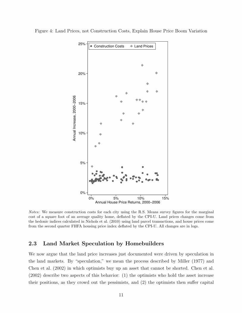
Figure 4: Land Prices, not Construction Costs, Explain House Price Boom Variation

0%

5%

10%

15%

20%

25%

Annual In

cre

ase, 2000−

2006

0% 5% 10% 15%Annual House Price Returns, 2000−2006

Construction Costs Land Prices

Notes: We measure construction costs for each city using the R.S. Means survey figures for the marginalcost of a square foot of an average quality home, deflated by the CPI-U. Land prices changes come fromthe hedonic indices calculated in Nichols et al. (2010) using land parcel transactions, and house prices comefrom the second quarter FHFA housing price index deflated by the CPI-U. All changes are in logs.

2.3 Land Market Speculation by Homebuilders

We now argue that the land price increases just documented were driven by speculation in

the land markets. By “speculation,” we mean the process described by Miller (1977) and

Chen et al. (2002) in which optimists buy up an asset that cannot be shorted. Chen et al.

(2002) describe two aspects of this behavior: (1) the optimists who hold the asset increase

their positions, as they crowd out the pessimists, and (2) the optimists then suffer capital

11

losses when their beliefs are revealed to be more optimistic than reality.

We document both of these features among a class of landholders for which we have rich

data: public homebuilders. These firms report their land holdings and losses on these land

holdings on their annual financial statements (10-Ks). We focus on the eight largest firms

over this period.8

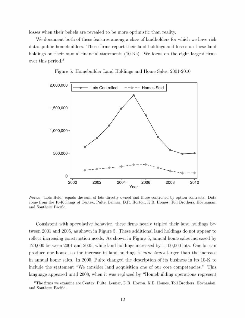
Figure 5: Homebuilder Land Holdings and Home Sales, 2001-2010

0

500,000

1,000,000

1,500,000

2,000,000

2000 2002 2004 2006 2008 2010Year

Lots Controlled Homes Sold

Notes: “Lots Held” equals the sum of lots directly owned and those controlled by option contracts. Datacome from the 10-K filings of Centex, Pulte, Lennar, D.R. Horton, K.B. Homes, Toll Brothers, Hovnanian,and Southern Pacific.

Consistent with speculative behavior, these firms nearly tripled their land holdings be-

tween 2001 and 2005, as shown in Figure 5. These additional land holdings do not appear to

reflect increasing construction needs. As shown in Figure 5, annual home sales increased by

120,000 between 2001 and 2005, while land holdings increased by 1,100,000 lots. One lot can

produce one house, so the increase in land holdings is nine times larger than the increase

in annual home sales. In 2005, Pulte changed the description of its business in its 10-K to

include the statement “We consider land acquisition one of our core competencies.” This

language appeared until 2008, when it was replaced by “Homebuilding operations represent

8The firms we examine are Centex, Pulte, Lennar, D.R. Horton, K.B. Homes, Toll Brothers, Hovnanian,and Southern Pacific.

12

our core business.”

Having amassed these large land portfolios, the firms we study then proceeded to suffer

large capital losses. Figure 6 documents the quite dramatic rise and fall in the total market

equity of these homebuilders between 2001 and 2010. The homebuilder stocks rose 430% and

then fell 74% over this period. These large changes are specific to these firms and not the

stock market generally. The S&P 500 index fell -2.5% from 2001-2005 and then fell -9.6%

from 2005 to 2010.

The majority of the losses from 2005 to 2010 borne by these homebuilders arise from

losses on the land portfolios they built up from 2001 to 2005. Starting in 2006, these firms

report write-downs to their land portfolios in their annual financial reports. We aggregate

these losses across firms, and report the total annual write-downs and the total annual market

equity losses in Table 2. The value of the land losses between 2006 and 2010, $29 billion, is

73% of the size of the market equity losses over this time period.

Figure 6: Homebuilder Market Equity, 2001-2010

0

20

40

60

Billio

ns o

f D

olla

rs

2000 2002 2004 2006 2008 2010

Year

Notes: Data come from the 10-K filings of Centex, Pulte, Lennar, D.R. Horton, K.B. Homes, Toll Brothers,Hovnanian, and Southern Pacific.

13

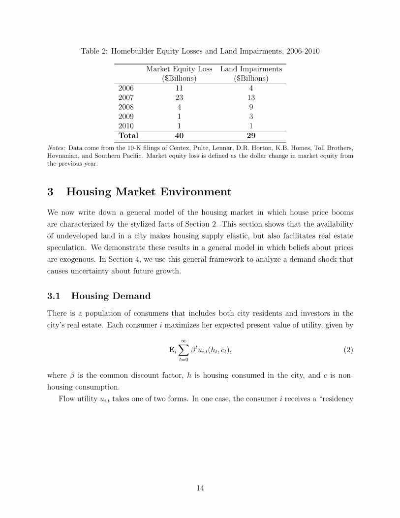
Table 2: Homebuilder Equity Losses and Land Impairments, 2006-2010

Market Equity Loss Land Impairments($Billions) ($Billions)

2006 11 42007 23 132008 4 92009 1 32010 1 1Total 40 29

Notes: Data come from the 10-K filings of Centex, Pulte, Lennar, D.R. Horton, K.B. Homes, Toll Brothers,Hovnanian, and Southern Pacific. Market equity loss is defined as the dollar change in market equity fromthe previous year.

3 Housing Market Environment

We now write down a general model of the housing market in which house price booms

are characterized by the stylized facts of Section 2. This section shows that the availability

of undeveloped land in a city makes housing supply elastic, but also facilitates real estate

speculation. We demonstrate these results in a general model in which beliefs about prices

are exogenous. In Section 4, we use this general framework to analyze a demand shock that

causes uncertainty about future growth.

3.1 Housing Demand

There is a population of consumers that includes both city residents and investors in the

city’s real estate. Each consumer i maximizes her expected present value of utility, given by

Ei

∞∑t=0

βtui,t(ht, ct), (2)

where β is the common discount factor, h is housing consumed in the city, and c is non-

housing consumption.

Flow utility ui,t takes one of two forms. In one case, the consumer i receives a “residency

14

shock” that compels her to live in the city at time t.9 In this case her utility is

ui,t(h, c) =

v(h) + aih+ c if owning h

v(h) + c if renting h,(3)

where v is an increasing, concave function for which v′(0) =∞, and ai is drawn from some

atomless distribution Fa whose support includes 0. If consumer i does not receive this shock,

then she is an “outsider” who derives no benefit from living in the city, and her utility is

given by

ui,t = c. (4)

The function v(·) represents intensive housing demand. In this context, owner-occupied

and rental housing are perfect substitutes. The parameter ai is a reduced form that captures

reasons some residents prefer owning to renting, or vice-versa. As we discussed in the Intro-

duction, explanations for this preference offered by the literature have relied on maintenance

costs, tax advantages, risk management, moving costs, and liquidity. We show in Section

7 that a moral hazard formulation, similar to Henderson and Ioannides (1983), in which

maintenance is not fully contractible can exactly generate the linear functional form used

here. Residents derive more flow utility from owner-occupancy when ai > 0, and more flow

utility from renting when ai < 0.

There are three assets consumers may hold: housing H, land L, and bonds b. Housing

and land cannot be shorted, and can only be held in non-negative quantities.10 A consumer’s

housing asset holding H need not equal her housing consumption level h. If H > h, then

the consumer is a landlord: she owns more housing than she consumes. If H < h, then

the consumer is a renter because she owns less housing than she consumes. If H = h, then

the consumer is an owner-occupant.11 In all three cases, the net rental income is rt(H − h),

where rt is the market rent for housing at time t.

Bonds are traded on a global market, and the gross interest rate Rt on bonds equals 1/β

9The extensive margin of living in the city is exogenous. This extensive margin can be added in and theresults stay the same. The difference is that the demand curve for housing that comes out of the modelhas a broader interpretation that includes both the intensive and extensive margin. What matters for ourresults is that this demand curve is smooth. The smoothness comes here from the continuity of housing,but it could also come from an extensive margin in which city amenities for each resident are drawn from acontinuous distribution.

10Shorting is impossible because of a lack of asset interchangeability in the real estate market that we donot model explicitly here. As explained in the Introduction, short sales are possible only when there existcomparable assets with which to cover one’s short. Land parcels and houses are all unique. In Section 7,we discuss the robustness of our results to the introduction of additional real estate securities, such as thehousing futures proposed by Shiller (1998), that allow investors to short the housing market indirectly.

11The resident may be an owner-occupant in addition to a landlord in the case H > h. The resident rentsout H − h units of housing, and owner-occupied the remaining h units.

15

for all t, where β is the common discount factor. Residents and outsiders can borrow or lend

in unlimited quantities (in the background is some income stream that guarantees that these

loans will always be repaid).12

Thus, consumers have five choices to make at time t. They choose their asset holdings

Ht and Lt of housing and land. They also choose their consumption levels of housing ht, as

well as non-housing consumption ct. Finally, they choose bond holdings bt. The resulting

Bellman equation corresponding to equation (2) is

V (Ht−1, Lt−1, bt−1) = (5)

maxht,ct,Ht,Lt,bt

ui,t(ht, ct)︸ ︷︷ ︸flow utility

+ βEiV (Ht, Lt, bt)︸ ︷︷ ︸continuation value

,

where the maximization is subject to the short-sale constraint

0 ≤ Ht, Lt (6)

and the budget constraint

pht (Ht −Ht−1)︸ ︷︷ ︸housing purchases

+ plt(Lt − Lt−1)︸ ︷︷ ︸land purchases

+ct ≤ rt(Ht − ht)︸ ︷︷ ︸rental income

+ bt −Rtbt−1︸ ︷︷ ︸bond income

, (7)

where pht and plt denote the prices of housing and land, respectively.

One feature of this set-up is that both residents and outsiders can invest in the land and

housing markets. This feature captures the behavior of many homeowners who purchased

second homes for investment purposes during the boom. Haughwout et al. (2011) examine

detailed credit data and conclude that 50% of the mortgages originated between 2004-2006 in

Arizona, California, Florida, and Nevada were to investors purchasing second homes; Bayer

et al. (2013) construct a similar measure and find that investment purchases comprised 30%

of home buying in Los Angeles. Of course, many of the investors in land markets were not

individual homeowners but large firms, as we documented in Section 2. Shareholders of such

firms are the outsiders in our model.

The number of consumers who receive the residency shock at time t is given by Nt.13

12The lack of credit constraints will mean that in markets where investors participate, the most optimisticinvestor will always hold all of the asset. In Section 7, we introduce a borrowing constraint to deriveadditional results about the effect of credit on the housing boom and bust.

13We only allow an intensive margin of housing choice. As house prices rise, residents buy smaller houses.In principle we could model an extensive margin where higher prices induce residents to move out of thecity. In each case we would get an aggregate demand curve that would be isomorphic and would not changeour results.

16

This aggregate housing demand evolves according to a stochastic process

logNt = logNt−1 + ζt. (8)

Residents (may) hold heterogeneous beliefs about future demand innovations ζt. Specifically,

the expectation Ei(ζt′ | ζt, ζt−1, ...) may vary across residents i for t′ > t. We will assume a

specific functional form for these innovations when we introduce the demand shock in Section

4, and will explain why heterogeneous beliefs are reasonable in the setting of that shock.

It is not necessary to specify the process through which individual consumers receive the

residency shocks. For example, it is not necessary to model any serial correlation in being

a resident. Consumers have quasi-linear utility in all states of the world, so their marginal

utility is always the same. Therefore, a consumer solving equation (5) does not care about

whether she is a resident or an outsider in future periods. The future prices of the assets she

holds are sufficient statistics for her welfare.14

3.2 Housing Supply

A unit of housing can be produced with one unit of land, plus a construction cost of C

(measured in terms of a composite commodity c with a price normalized to 1). A Leontief

production function captures this cost structure and is given by

H = min(L, c/C). (9)

Housing construction is irreversible, and the housing stock does not depreciate. Construction

is performed by a perfectly competitive industry of homebuilders.15

The only constraint on housing supply is a long-run constraint on the total amount of land

in the city, which we denote L. This development constraint reflects a variety of barriers to

unlimited growth that cities or neighborhoods face. Saiz (2010) documents how geography

(e.g. mountains and water) limits the growth of metropolitan areas. Often development

restrictions are man-made, taking the form of zoning and “growth management” policies

that manage the long-term size of a city or neighborhood.16 A final source of this constraint,

14Quasi-linear utility eliminates risk aversion and any hedging motives for owning versus renting housing.Household risk management is clearly important. Piazzesi et al. (2007) provide an asset pricing modelin which housing and other consumption are non-separable and individuals are risk-averse, and Sinai andSouleles (2005) show that owning housing acts as a hedge against future rent risk. Abstracting from theseconsiderations allows us to focus on the precise role that flow utility plays in aggregating resident and investorbeliefs.

15The largest 100 builders had less than 45% market share in each year from 2001-2006, according toMartin and Whitlow (2012), which draws data from Builder Magazine.

16These regulations also restrict the amount of housing that can fit on a parcel of land. Therefore, it most

17

which we do not explicitly model, is transportation costs that establish a commuting radius

around a city center. Even with no geographic or regulatory constraints, the scope of a city

will be limited if all residents have to commute to the same central location each day, and

commuting takes time that scales linearly with distance.

One feature of this approach is that the short-run supply elasticity will be endogenous to

the model, depending on the city’s level of development relative to the long-run constraint.

The literature on housing supply (Topel and Rosen, 1988; Saiz, 2010; Glaeser et al., 2013)

largely assumes an exogenous static supply elasticity, which may vary across cities. Our

set-up generalizes this formulation by jointly modeling the short-run supply elasticity and

land prices.

Another feature of our production function is constant construction cost C. The constant

construction cost setting allows us to clearly explain how a housing boom can occur in an

area with no short-term barriers to construction. Furthermore, as discussed in Section 2 and

shown in Figure 4, constant construction costs largely corresponds to the cross-city housing

boom experience in the latest U.S. housing episode.

As we explain below, short-run housing supply will be perfectly elastic when land remains

for construction, and perfectly inelastic when all land has already been used for housing. In

reality, even very dense areas experience some housing construction, and cities do not face

such a discontinuous transition from having perfectly elastic to perfectly inelastic housing

supply. A simple extension to our model, which we discuss in Section 7, addresses both

points. We allow land to have a productive use other than house construction which enters

the resident utility function. As long as an Inada condition is satisfied, then these unrealistic

discontinuities disappear, but our main results are preserved.

3.3 Equilibrium

Equilibrium holds when consumers are optimizing, the construction industry is operating at

cost, and housing and land markets clear:17

Definition 1. Let H∗i (pht , plt, rt), L∗i (p

ht , p

lt, rt), and h∗i (p

ht , p

lt, rt) denote the solutions to the

Bellman equation (5). Then prices pht , pqt , and rt constitute an equilibrium if the following

natural to think of L as a three-dimensional constraint that restricts the total amount of housing that canbe built in an area, including vertically.

17The equilibrium condition we provide for builder optimization is that house prices equal land prices plusconstruction costs. This condition holds as long as housing demand does not fall too much relative to theexisting housing stock, creating an “over-building” scenario. As our attention is on the boom and not thebust, we choose not to focus on this case. Our results hold as long as optimistic investors who price theassets believe that the city will not be in this over-building scenario in the subsequent period.

18

market-clearing conditions hold:

housing market:∑i

H∗ =∑i

h∗i ; (10)

land market: L =∑i

H∗ +∑i

L∗; (11)

and if the competitive construction industry makes zero profits:

pht = plt + C. (12)

We denote the housing stock at time t by H t:

H t ≡∑i

H∗t . (13)

There are three broad points about the equilibrium we would like to make in this general

setting. The first is that house prices can be written as the sum of current and future rents.

We can specifically write

pht = rt + βEpht+1, (14)

where E represents the beliefs of residents and outsiders who are landlords. This equation

results from landlord arbitrage: they must be indifferent between selling their houses and

renting them out.

The second point is that the equilibrium falls into two cases: when demand is high, all

land is used for housing, and when demand is low, some land remains undeveloped. This

dichotomy will be quite important for analyzing the model, so it is worth spending some

space building up the intuition with equations. The basic idea is that when housing demand

is high, it is inefficient to let any land sit idle, so investors build houses on the land and

sell them to residents. To see this, consider the first-order condition for resident housing

consumption:

0 = max(v′(h∗)− rt, v′(h∗)− (pht − βEipht+1 − ai)) (15)

If the first argument is larger, the resident rents, and if the second argument is larger, the

residents owns. We let D ≡ (v′)−1 denote each resident’s demand curve for housing. We can

19

substitute (14) into (15) to derive the market-clearing condition

H t =

rental demand︷ ︸︸ ︷∑ai<β(Epht+1−Eipht+1)

NtD(rt) +

owner-occupancy demand︷ ︸︸ ︷∑ai>β(Epht+1−Eipht+1)

NtD(rt − ai + β(Epht+1 − Eip

ht+1)),

(16)

where H t is the stock of housing. When this total demanded housing stock H t is less than

the total land supply L, some raw land remains. The total stock demanded depends on

aggregate demand Nt and market rents rt. Market rents, however, are pinned down by

construction costs when land remains. If land remains, then a landowner must be indifferent

between building a house and selling today or doing the same tomorrow. Therefore, pht −C =

β(Epht+1 − C); together with equation (14), this arbitrage condition means that

rt = (1− β)C (17)

when raw land remains. The quantity (1− β)C equals the “flow costs” of construction, i.e.

the costs of building today as opposed to next period.

The level of demand N∗t at which all land is used for housing is the level at which housing

demand given by (16) equals the total land L when rents equal rt = (1 − β)C. When Nt

is below this threshold, the amount of housing demanded when it is suppled at cost is not

enough to fill up the city. When Nt is above this threshold, the amount of housing demanded

when it is supplied at cost exceeds the space available in the city. Lemma 1 summarizes this

result.

Lemma 1 (Land Exhaustion). There exists a level of aggregate demand N∗t such that when

demand Nt exceeds this threshold, all land is used for housing: H t = L. When demand Nt

falls short of this threshold, some land remains undeveloped: H t < L.

The third point and final point is that pass-through of demand shocks to prices is higher

when demand is higher, but the pass-through of investor beliefs to prices is higher when

demand is lower. Speculation has the largest impact on prices precisely when the elasticity

of housing supply is high.

Let us turn first to the direct effect of a demand shock on prices and housing quantities.

Recall that an innovation to log housing demand logNt is given by ζt, as specified by equation

(8). In theory this innovation can affect future price expectations because it may convey

information about future shocks. Here we will consider just the direct effects of the shock ζt

holding future price expectations constant.

The effect of the shock ζt on house prices and quantities is actually quite simple in our

20

model. We can most easily describe the effect of the shock by examining the city in the two

separate cases of full development (Nt > N∗t ) and continuing development (Nt < N∗t ).

By assumption, the shock we are considering does not affect future price expectations,

and therefore affects prices only through current rents rt (see equation (14)). When Nt < N∗t ,

these rents are fixed at the flow construction cost rt = (1− β)C (equation (17)). Therefore,

the shock ζt has no affect on rents when the city is undeveloped. Furthermore, the shock

passes through to quantities 1-for-1 in this undeveloped case. The housing demand equation

(16) may be written H t = NtDt(rt), where Dt aggregates individual housing demands D.

Because rt is fixed, innovations in Nt pass through perfectly to the housing stock H t.

The effect of the shock is completely the opposite when the city is fully developed (Nt >

N∗t ). Now, the housing stock is fixed at H t = L, the amount of space available. The shock

therefore has no effect on housing supply. In contrast, rents are no longer fixed, and are

determined by the market-clearing equation (16) with the housing stock fixed at L. We

may write this condition as L = NtDt(rt). Differentiating this equation with respect to a

log change in Nt yields ∂ log rt/∂ζt = 1/εt, where εt is the elasticity of demand Dt given by

εt = −rtD′t(rt)/D(rt).

Proposition 1 summarizes these results.

Proposition 1 (Supply-and-Demand Effect of Land). Consider a shock ζt to demand logNt

that does not affect beliefs about future shocks. The shock raises house prices if and only if

all land is being used for housing. The shock leads to new construction if and only if some

of the land is still undeveloped. The shock affects house prices only through rents, and its

affects on house quantity H t and rents rt are given by

∂ logH t

∂ζt=

1 if Nt < N∗t

0 if Nt ≥ N∗t

(18)

∂ log rt∂ζt

=

0 if Nt < N∗t

1/εt if Nt ≥ N∗t ,(19)

where Nt is the level of housing demand, and N∗t is the threshold at which the city fully

develops given by Lemma 1.

Proposition 1 states the classic supply-and-demand theory of a housing boom. When land

is still available, housing supply is completely elastic (pass-through is unity), and the shock

has no affect on house prices. When land is no longer available, housing supply is completely

inelastic (pass-through is 0), and the shock raises rents according to a demand elasticity.

Land availability means that housing supply is more elastic and demand shocks have smaller

21

effects on prices.

Land availability has exactly the opposite effect on the pass-through of investor beliefs to

house prices. As we now show, land availability facilitates speculation, allowing speculators

to raise prices more. Again, the analysis proceeds most logically if we separately consider

the case where land is available and the case where all land is used for housing.

When all land is used for housing, landlords face frictions from trying to rent out “too

much” of the housing stock. There is a natural market for renting, namely the residents for

whom ownership utility ai is negative. If landlords buy up more housing than they can rent

to these residents, they exert downward pressure on rents, cutting into their returns.

To show how this friction emerges from the model, we differentiate (16) with respect to

the discounted investor belief βEpht+1, keeping in mind that H t is fixed. What we obtain is

∂rt

∂βEpht+1

= −

∑ai>β(Epht+1−Eipht+1)

D′i∑aiD′i

, (20)

where Di(rt) ≡ D(rt) if ai < β(Epht+1−Eipht+1) and Di(rt) ≡ D(rt− ai + β(Epht+1−Eip

ht+1))

otherwise. Equation (20) can be given an intuitive interpretation. It is, on the margin, the

fraction of the housing market that is owner-occupants. When speculative investors buy up

housing, they push up prices, leading to expected capital losses for owner-occupants. On the

margin, the rental and owner-occupied populations are distinct (substitution effects between

groups are second-order). Therefore, for the housing market to clear, rents must fall to offset

the lower demand from owner-occupants coming from expected capital losses.

We may substitute (20) into (14) to derive the total effect of speculators on house prices

when the housing stock is fixed:

∂pht∂βEpht+1

=

rental market depth︷ ︸︸ ︷∑ai<β(Epht+1−Eipht+1)

D′i∑ai

D′i︸ ︷︷ ︸total market depth

≡ χ. (21)

The price effect of speculators is between 0 and 1. If all of the market is rental housing, then

their beliefs pass through 1-for-1 to prices. If all of the housing is owner-occupied, they have

no effect on house prices.

In contrast, investor beliefs pass through 1-for-1 to house prices when land is still avail-

able. To see this, we need only combine equations (14) and (17). Rents are fixed when land

22

is still available. Therefore, investor beliefs pass-through completely to house prices.

Intuitively, investor beliefs determine land prices without any frictions, because they

do not need to rent out land to capture its value. But house prices are determined by land

prices: to build a house, a homebuilder must buy land from one of these optimistic investors.

This argument only holds when investors are holding land in equilibrium. If demand is high

(Nt > N∗t ), it is always more efficient for investors to build on their land than to hold it, and

investor no longer price the land as they do when demand is low.

Proposition 2 summarizes these results.

Proposition 2 (Speculation Effect of Land). When rental frictions are present (χ < 1),

speculative investors affect house prices more when undeveloped land remains than when the

city is fully developed. The pass-through of investor beliefs to house prices is given by

∂pht∂βEpht+1

=

1 if Nt < N∗t

χ if Nt ≥ N∗t ,(22)

where χ ∈ (0, 1) is the ratio of rental market depth to total market depth given by equation

(21), Nt is the level of housing demand, and N∗t is the threshold at which the city fully

develops given by Lemma 1.

Proposition 2 shows that the effect of speculation on prices is perfectly negatively correlated

with the direct effect of a demand shock on prices given by Proposition 1. Speculation has

the largest effect on prices when the city is undeveloped. The direct effect of a demand shock

on prices is smallest when the city is undeveloped, and in that case the supply response is

the largest.

One shortcoming of our approach so far is that we have taken investor beliefs Epht+1 to

be exogenous, in particular not to depend on the level of development Nt. This level of

generality has allowed us to derive broad results about the relationship between housing

supply and speculation in real estate markets. In order to close the system, we turn now to

a model of a housing boom and bust in which specify beliefs more carefully.

4 Housing Boom

4.1 Demand Shock and Beliefs

Our goal is to consider the types of housing booms described by Glaeser (2013). In his

account, the hallmarks of a housing boom and bust are an initial period of surging hous-

ing demand that coincides with uncertainty about future housing demand, followed by a

23

subsequent period in which that uncertainty is resolved. To match this framework, we em-

bed a simple two-period model of uncertainty the dynamic model of the housing market we

developed in Section 3.

The period of the initial shock is t = 0. Before this period, all residents and outsiders

agree about the future housing market. At time 0, log housing demand rises unexpected by

x:

logN0 = x+ E logN0, (23)

where E denotes the common, time t = −1 expectation of residents. The arrival of this shock

creates new uncertainty about future housing demand. In particular, consumers disagree

about the shock’s persistence, that is, whether the current shock x indicates that future

housing demand will also rise. Resident i’s perceived persistence is µi, so that

Ei logNt = µix+ E logNt, (24)

where E again denotes the common, time t = −1 expectation of residents. At time t = 1,

residents learn the true value of this persistence µ. The shock x and the resultant uncertainty

are unanticipated by residents at time t = −1.

As in several recent finance papers,18 the actors in our model “agree to disagree,” in this

case about µ. They form their beliefs solely on the basis of subjective priors, and draw no

inferences from the actions of other residents. As argued by Morris (1996), this heterogeneous

prior assumption is most appropriate when investors face an unprecedented situation in which

they have not yet had a chance to collect information and engage in rational updating. The

events surrounding housing booms are precisely these types of situations. Glaeser (2013)

takes great pains to show that in each of the historical boom episodes he analyzes, reasonable

investors could agree to disagree about future real estate prices. In the case of the 2000-2010

housing boom and bust, we follow Mian and Sufi (2009) in thinking of the shock x as the

arrival of new securitization technologies that expanded credit to low-income borrowers. The

µ in our model reflects the degree to which this expansion of credit in 2000-2006 persisted

after 2006.

Because disagreement about µ is resolved after a single period of uncertainty, residents

have no incentive to forecast the beliefs of other residents. The “resale option” effect of

Harrison and Kreps (1978) and Scheinkman and Xiong (2003) in which residents buy an

asset to sell it to a future optimist is absent here.19

18See Geanakoplos (2009), Simsek (2013), and Brunnermeier et al. (2013).19Our set-up also differs from Scheinkman and Xiong (2003) in the sense that residents do not infer any

information from other residents, whereas invests in Scheinkman and Xiong (2003) only update partially fromthe actions of others. Our residents are like the investors in that paper if they had infinite overconfidence.

24

4.2 Future Price Expectations

The shock parametrization we have just written down lets us solve for the future price

expectations Eiph1 that we treated as exogenous in Section 3. Because we are interested in

the effect of the shock x on house prices, it is sufficient to calculate the derivative ∂Eiph1/∂x,

as opposed to computing the level of this expectation.

A helpful decomposition is to write ph1 as the sum of rents:

ph1 =∞∑j=0

βjrj+1. (25)

Consumer i believes that the shock will raise log housing demand logNt by µix in all future

periods. By Proposition 1, this future shock will have no effect on rents in the future periods

in which the city is undeveloped, and will raise log rents by 1/εt in future periods where the

city is developed. The development cutoff in all future periods N∗t is the same because all

residents have the same beliefs in those periods; we denote it N∗.20 Therefore, the future

shock raises rents only in periods in which Nt > N∗. The total effect of the shock on future

price expectations is the fraction of the city’s future that is constrained times the average

elasticity in those periods. Lemma 2 states this result precisely.

Lemma 2 (Long-Run Constraint Measure). The effect of the shock x on resident i’s future

price expectation is∂ log Eip1

∂x=ρµiεc0. (26)

Here ρ ∈ [0, 1] is the fraction of future rents that accrue when the city is constrained:

ρ ≡∑

j≥J βjrj∑

j≥1 βjrj

, (27)

where J = min(j | Nj > N∗) is the number of periods until the city runs out of land.21 The

term εc0 is the average elasticity of housing demand in the city’s constrained future:

εc0 ≡

(∑j≥J β

jrj/εj∑j≥J β

jrj

)−1. (28)

20In equation (16), the term Epht+1−Eipht+1 = 0 for all i when residents hold the same beliefs. Therefore,

the solution N∗ to the equation L = NtD((1− β)C) does not depend on t.21This formulation assumes that once the city runs out of land, it never can tear down houses and re-enter

the state in which land remains. This result holds if house construction is irreversible or if demand Nt isalways increasing for t ≥ 1.

25

Lemma 2 shows how the long-run constraints play a role in future price expectations.

The parameter ρ describes how supply-restricted the city is in the long-run, on a scale from

0 to 1. At ρ = 0, the city has enough land to develop for decades (in fact for eternity), and

so whether the shock x persists is irrelevant for future prices. In this case, the speculation

goes away, even though there is ample land which investors can use for trading. The reason

is that future prices are completely certain when the city will never run out of land; house

prices equal construction costs C for the foreseeable future.

Larger values of ρ that are less than 1 correspond to cases in which the city is approaching

its long-run development constraint. An example would be Las Vegas as depicted in Figure

2 in the Introduction. Half of the available land had been developed in 2008, and at its

recent growth rate, Las Vegas would use up the remaining land in the next 10-20 years. A

back-of-the-envelope calculation suggests that a reasonable value for ρ in this setting is 0.5.

The larger ρ, the greater the scope for disagreement about future house prices.

Finally, ρ = 1 when a city is already fully developed.

4.3 Impact of Shock on Prices

We now put together the general results of Section 3 with the characterization of future price

expectations of Lemma 2 to derive the effect of the shock on house prices at time 0.

The shock has two effects on prices. First, it affects current rents through the supply-

and-demand channel explained in Proposition 1. The shock raises log demand by x at time

0; this demand shock raises rents today if the city is fully developed and does not raise rents

if the city still has raw land.

The shock also affects prices by changing expectations Eiph1 of future prices, which are

embedded in today’s price ph0 . Proposition 2 shows that when the city is undeveloped,

investor beliefs solely determine the future price expectations capitalized into prices at time

0. Following the notation used in Section 3, we denote the investor belief about µ by µ.

When the city is fully developed, investors face frictions in the housing market, and their

beliefs no longer fully determine prices. Proposition 2 shows that their beliefs account only

for a fraction χ of the beliefs capitalized into prices at time 0. The remaining 1−χ comprise

the beliefs of the owner-occupants who are also holding housing. We have not formally proved

this result yet, but it follows easily from the general market-clearing condition for housing

given in equation 16 in Section 3. We take the derivative of this equation with respect to

each owner-occupant’s belief Eipht+1 and then aggregate these effects appropriately over all

26

owner-occupants. What we find is that

∂rt

∂βEpht+1

= 1− χ, (29)

where χ is given by equation (21) and Epht+1 is the average owner-occupant belief given by

Epht+1 ≡

∑ai>β(Epht+1−Eipht+1)

Eipht+1D

′i∑

ai>β(Epht+1−Eipht+1)D′i

. (30)

We let µ denote the average owner-occupant belief about µ that comes from substituting

the expression for Eip1 from Lemma 2 into equation (30).

Putting together the speculation effect and the supply-and-demand effect we have just

discussed yields the total effect of the shock x on house prices ph0 . Following the Lemmas and

Propositions up to this point, we express this effect as a change in log prices log ph0 . Doing

so creates one new log-linearization parameter, λ, which expresses the share of house prices

attributable to current rents instead of to future price expectations.22

Proposition 3 (Price Impact of Shock). Consider a shock that raises current housing de-

mand logN0 by x and future demand by µx, where µ has an uncertain value about which

consumers disagree. The total effect of this shock on house prices ph0 at time 0 is given by

∂ log ph0∂x

=

future price expectations︷ ︸︸ ︷(1− λ)

ρµ

εc0if Nt < N∗t

λ1

ε0︸︷︷︸current rents

+ (1− λ)χµ+ (1− χ)µ

εc0︸ ︷︷ ︸future price expectations

if Nt ≥ N∗t ,

(31)

where Nt is the level of housing demand, and N∗t is the threshold at which the city fully

develops given by Lemma 1. Only the optimistic investor belief µ matters when undeveloped

land remains in the city. When the city is fully developed, the average belief of owner-

occupants µ matters in addition to the investor beliefs, as long as rental frictions are present

(χ < 1). The shock raises current rents only when the city is fully developed.

We put off analyzing this result until we have derived a similar expression for construction.

This result will allow us to compare the size of the housing boom in different types of cities.

22More precisely, λ = r0/ph0 conditional on the shock x = 0, and satisfies ∂ log ph0/∂x = λ log r0/∂x+ (1−

λ)∂ logEph1/∂x.

27

4.4 Impact of Shock on Quantities

We began this paper by describing why high construction housing booms are a puzzle. To

explain this puzzle, we analyze the effect of the shock x on construction, supplementing the

formula we just gave for the shock’s effect on prices. The construction caused by the shock

is given by the shock’s effect on the level of the housing stock at time 0, H0.

As in our analysis of prices, the shock x has two effects on house quantities, corresponding

to the current effect of the shock x at time 0 and the changes in beliefs about future demand.

The direct effect at time 0 is like the demand shock ζt considered in Proposition 1. It passes

through 1-for-1 to quantities when land remains, but has no effect on construction when the

city is fully developed.

Speculation in land markets also has an effect on construction. We have not considered

this effect up until now, but it comes out of the equations we have written down. More

intense speculation in land markets (i.e. higher values of µ, or Epht+1 in the general model)

curtails construction. The reason is that this speculation raises house prices, making housing

more expensive for owner-occupants and decreasing the amount of housing they demand. To

derive this effect, we differentiate the market-clearing equation (16) with respect to investor

and owner-occupant beliefs, and then substitute equations (26), (30), and the definitions of

the demand elasticity ε0 and the log-linearization parameter λ.23 The result is Proposition

4.

Proposition 4 (Quantity Impact of Shock). Consider a shock that raises current housing

demand logN0 by x and future demand by µx, where µ has an uncertain value about which

consumers disagree. The total effect of the shock x on the housing stock H0 at time 0 is

given by

∂ logH0

∂x=

1−

construction attenuation︷ ︸︸ ︷ε0εc0

1− λλ

(µ− µ)ρ(1− χ) if Nt < N∗t

0 if Nt ≥ N∗t ,

(32)

where Nt is the level of housing demand, and N∗t is the threshold at which the city fully

develops given by Lemma 1. The shock increases construction when undeveloped land remains

23Differentiating the market-clearing equation (16), noting that r0 stays constant at (1 − β)C, yields∂H0/∂x =

∑N0D

′i(∂βEp

h1/∂x−∂βEip

h1/∂x), where the sum is taken just over owner-occupants. Factoring

out∑N0D

′i, diving both sides of the equation by H0, and using the definition of χ given by equation (22)

transforms this equation to ∂ logH0/∂x = (1 − χ)(D′0/D0)(∂βEph1/∂x − ∂βEph1/∂x), where D0 is the sumof all resident demands Di and E is the average owner-occupant belief given by equation (30). Finally, wemultiply by 1 = r0(βEph1/r0)/(βEph1 ), where E denotes the common expectation before the shock that holdswhen x = 0, to reduce the last equation to ∂ logH0/∂x = (1 − χ)(ε0/ε

c0)(µ − µ)ρ(1 − λ)/λ, in which we

use the definition ε0 ≡ rD′0/D0, the formula (26) for the effect of the shock on belief, and the definitionλ = r0/(r0 + βEph1 ).

28

as long as the current housing demand elasticity ε0 is small relative to the demand elasticity

εc0 in the future when the city is developed. The shock has no effect on construction in fully

developed cities.

We call the negative term “construction attenuation” because it shows that the con-

struction response to the shock x is curtailed. In principle, this term could lead a city with

undeveloped land not to meet the shock with very much construction. However, we are

skeptical that this term is of much empirical relevance. The reason is that this term is small

when ε0/εc0 is small, that is, when housing demand is more inelastic when house prices are

cheap. The term ε0 represents housing demand elasticity when housing is cheap (rents equal

construction costs (1−β)C), and εc0 represents housing demand elasticity in the future when

the city is constrained and rents become expensive. We imagine a world in which most

residents receive consumer surplus from cheap housing. In this case, very few residents are

on the margin when housing is cheap, but residents start getting rationed out of an area

when rents begin to rise. In this case, ε0/εc0 will be small.

We now use Propositions 3 and 4 jointly to analyze housing booms in different types of

cities.

4.5 A Tale of Three Cities

In this section, we show that the joint behavior of prices and quantities can be usefully

described as falling into one of three possibilities, which depend on the level of development

of the city. The first city is one that has an unlimited amount of land for future development.

The second city is one which is still developing, but will run out of available space soon. The

final city is one that has already fully developed. As we will show, high construction housing

booms occur precisely in the intermediate case.

4.5.1 City 1: Unlimited Land

In the first type of city, the available space L is very large relative to Nt. Land remains for

development, and will continue to remain for the foreseeable future. The parameter ρ, which

measures how supply-restricted the city is in the long-run, equals 0.

Propositions 3 and 4 show that the effect of the shock on prices is 0, while the shock

passes through perfectly to quantities: ∂ log ph0/∂x = 0 and ∂ logH0/∂x = 1. The unlimited

amount of land means that house prices just equal construction costs C at all times. They

don’t depend on current or future housing demand. By the same token, the city can always

accommodate additional housing demand buy building new houses.

29

These results correspond perfectly to the classic supply-and-demand intuition. In a lo-

cation with no current or future restrictions on housing supply, house prices stay constant

and construction can absorb all shocks.

In practice, a city or neighborhood that can be characterized as having unlimited land

must have some of the following features. First is a perceived lack of future regulation.

Investors must believe that future regulators will not prohibit housing supply. The second

feature is flat geography. If the city can expand forever, then there cannot be natural

barriers such as water or mountains on the horizon. Finally, a city with unlimited land in

this framework likely involves homogeneous sprawl. Sprawl means that commuting time does

not limit the growth of the metropolitan area, because workers are able to work near their

homes instead of in a central business district. Furthermore, within sprawl, neighborhoods

are good substitutes for each other, meaning that individual neighborhoods are not land-

constrained.

In the recent national housing boom and bust, we think of the sprawling metropolitan

areas of Texas as prime examples of locations with unlimited land. These areas are charac-

terized by flat geography, a history of low levels of regulation, and sprawl. They experienced

very small booms and busts and high levels of construction.

4.5.2 City 2: Approaching the Constraint

The second type of city is one in which undeveloped land is still present, but will be exhausted

in the future. The level of available space L relative to demand Nt is smaller than in the

previous type of city, but it is still large enough that raw land remains. The value of the

long-run development measure ρ in the city we are now considering is positive.

Propositions 3 and 4 show that a high construction housing boom occurs in this sort of

city. The price boom equals ∂ log ph0/∂x = (1 − λ)ρµ/εc0. This boom reflects the beliefs of

optimistic investors about future housing demand. Construction also booms. Proposition 4

shows that when demand is relatively inelastic, the present shock passes through completely

to construction: ∂ logH0/∂x = 1. When demand is more elastic, some of this construction

response is attenuated.

The boom in this area occurs purely through the speculation channel. Optimistic in-

vestors speculate in the land markets about future housing demand, pushing up house prices

today. Note that only the beliefs of the most optimistic investors matter for house prices,

because these are the investors who are holding the land (and for whom µi = µ). Speculation

means that house prices in this city are governed by the beliefs of a few fringe optimists who

can take large positions in the land markets.

One implication of this result in particular is that homeowner beliefs are irrelevant for

30

prices. Only the beliefs of real estate investors matter, and only the most optimistic beliefs

at that. Surveys of homeowner beliefs, such as Case et al. (2012), are actually uninformative

about house prices in this type of city. More useful would be surveys of the investors who hold

the land. A promising area of future research is to measure these beliefs using the National

Association of Homebuilder surveys of homebuilder sentiment, as these homebuilding firms

were prominent land investors during the recent boom.

The available land allows the city to accommodate the current demand shock x in new

construction. As long as homeowner demand is inelastic at the low initial price levels in the

city, homeowners do not balk at the rising prices wrought by the optimist investors, and

construction is high.

It is useful to walk through the anatomy of the boom in a specific example, given that

describing high construction housing booms is the motivation of the paper. We focus on Las

Vegas during the recent episode.

Around 2000, new technologies are developed that expand credit to low-income borrowers,

raising housing demand throughout the country and in Las Vegas. Due to the regulations

described in the Introduction and shown graphically in Figure 2, Las Vegas will run out of

land in the next 20-30 years. Investors, anticipating this future development, scramble to get

a hold of this remaining land, knowing that it will appreciate as the city continues to develop.

These land investments are akin to buying property in an up-and-coming neighborhood

before it gets popular. In Las Vegas, the belief was that once it ran out of land, it would

transition to being a glamorous, expensive city akin to those in coastal California from which

many of its migrants came. The mayor of North Las Vegas summed up this perception in

2007, when he said

I believe in 100 years they’ll be studying this [boundary] as a great piece of public

policy. I think it will go right up beside Robert Moses building New York.24

Investors disagree about Las Vegas’s future transition to an expensive city. They specu-

late in the land market, where speculation occurs quite easily because there are no frictions.

The most optimistic investors buy up all of the land, driving up land prices. House prices

rise because they are tied to land prices. Construction is high because the current subprime

shock, which got everyone speculating in the first place, has increased housing demand,

which builders can meet by building on the available land. Homeowners were getting a lot of

consumer surplus from the cheap housing, so they continue to buy as prices rise. People were

moving from California to Las Vegas because Las Vegas was much cheaper than California.

The higher prices just made Las Vegas housing seem like a good deal, instead of an excellent

24Quotation comes from McKinley and Palmer (2007).

31

one. Consistent with this intuition, Las Vegas led all metropolitan areas in construction

rates between 2000 and 2006.

Eventually, the surging housing demand starts to revert. Mian et al. (2013) provide

evidence that various measures of consumer credit health fell between 2006 and 2009. We

think of this period as the time in which the true value of the persistence of the initial shock

is revealed. Optimistic investors learn that the truth is less rosy than the one behind their

valuations of land, and land and house prices fall, causing the bust.

The general take-away from this specific example is that approaching a development

constraint is the necessary setting for a high construction housing boom. The upcoming

constraint creates uncertainty, leading to speculation in land markets. These same land

markets accommodate new construction. As we now discuss, both speculation and new

construction go away in the final city we consider, the fully developed one.

4.5.3 City 3: Fully Developed

The final category of city is the fully developed one in which no raw land remains. The level

of available space L is low relative to demand Nt.

Proposition 4 shows that there is no construction in this city. All available space already

has houses on it, so no additional construction is possible. Proposition 3 shows that there is

a house price boom, consisting of two effects: the direct effect on rents λ/ε0, and the effect

on future price expectations (1− λ)(χµ+ (1− χ)µ)/εc0. As in the city with unlimited land,

the housing boom here corresponds well to the predictions of the classic supply-and-demand

story.

What is notable about the boom in this city is that the beliefs that are capitalized into

prices are less optimistic than the beliefs in the developing city we just considered. In this

fully developed area, investors have only the housing markets; there are no land markets

for speculation. Optimistic investors can only partially effect prices. This partial effect is

represented by χ, the depth of the rental market relative to the entire housing market. The

larger the market for rental housing, the smaller the frictions and the more direct the effect

of speculators on prices.

The total market belief is χµ+ (1− χ)µ. It combines the average owner-occupant belief

and the optimistic investor belief. This combination is less affected by the beliefs of an

optimistic fringe. The non-transferable ownership utility means that home ownership is

dispersed in equilibrium among many individual residents. Their aggregate belief is given

by µ, and it guarantees that the market belief cannot get too optimistic.

The boom in this area is more about fundamental supply-and-demand than about spec-

ulation by optimistic investors. When rental frictions are complete (χ = 0), no speculation

32

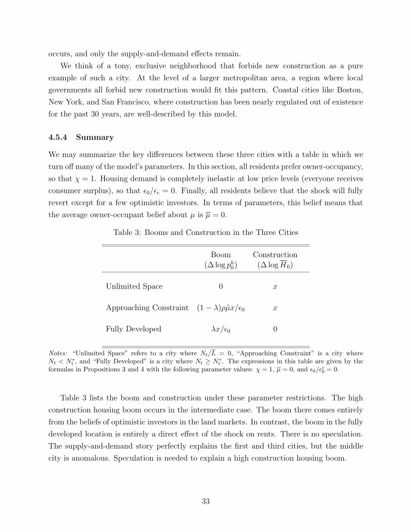
occurs, and only the supply-and-demand effects remain.

We think of a tony, exclusive neighborhood that forbids new construction as a pure

example of such a city. At the level of a larger metropolitan area, a region where local

governments all forbid new construction would fit this pattern. Coastal cities like Boston,

New York, and San Francisco, where construction has been nearly regulated out of existence

for the past 30 years, are well-described by this model.

4.5.4 Summary

We may summarize the key differences between these three cities with a table in which we

turn off many of the model’s parameters. In this section, all residents prefer owner-occupancy,

so that χ = 1. Housing demand is completely inelastic at low price levels (everyone receives

consumer surplus), so that ε0/εc = 0. Finally, all residents believe that the shock will fully

revert except for a few optimistic investors. In terms of parameters, this belief means that

the average owner-occupant belief about µ is µ = 0.

Table 3: Booms and Construction in the Three Cities

Boom Construction(∆ log ph0) (∆ logH0)

Unlimited Space 0 x

Approaching Constraint (1− λ)ρµx/ε0 x

Fully Developed λx/ε0 0

Notes: “Unlimited Space” refers to a city where Nt/L = 0, “Approaching Constraint” is a city whereNt < N∗t , and “Fully Developed” is a city where Nt ≥ N∗t . The expressions in this table are given by theformulas in Propositions 3 and 4 with the following parameter values: χ = 1, µ = 0, and ε0/ε

c0 = 0.

Table 3 lists the boom and construction under these parameter restrictions. The high

construction housing boom occurs in the intermediate case. The boom there comes entirely

from the beliefs of optimistic investors in the land markets. In contrast, the boom in the fully

developed location is entirely a direct effect of the shock on rents. There is no speculation.

The supply-and-demand story perfectly explains the first and third cities, but the middle

city is anomalous. Speculation is needed to explain a high construction housing boom.

33

4.6 Where is the Boom the Largest?

Because of frictions in the rental market encapsulated by χ, speculation can affect prices more

in undeveloped areas than in fully developed ones. If investors are sufficiently optimistic, this

speculative effect can overwhelm the direct effect of the shock on rents in the fully developed

areas. The price boom can actually be larger in undeveloped areas that have relatively more

land. To see this result, we need only turn to Proposition 3. The value of ρ can get as high

as 1 in unconstrained areas as they approach the development barrier. Therefore, there are

undeveloped areas with a boom exceeding the one in the fully developed cities if the top

term in equation (31) exceeds the bottom two terms when ρ = 1. Proposition 5 states the

condition under which this result holds.25

Proposition 5 (Boom Increases with Land Float). Consider a shock that raises current

housing demand logN0 by x and future demand by µx, where µ has an uncertain value

about which consumers disagree. If there are frictions in the rental market (χ < 1), then

the housing boom is largest in undeveloped areas when there is sufficient dispersion of beliefs

about µ. If

(1− χ)(µ− µ) > λ/(1− λ), (33)

then there exists N∗∗t < N∗t such that the boom is larger for N∗∗t < Nt < N∗t than for

Nt ≥ N∗t . Here Nt is the level of housing demand, and N∗t is the threshold at which the city

fully develops given by Lemma 1.

The intuition of Proposition 5 can be gleaned most readily from Table 3. In the special

case shown there, the boom in the intermediate city is larger than in the fully developed city

as long as the investors are optimistic enough. These investors are crowded out of the fully

developed city because of rental frictions.

Usually, we think that asset float decreases volatility from speculation. The usual logic,

offered for instance by Hong et al. (2006), is that larger float allows pessimists to participate,

blunting the effect of optimists and attenuating price volatility. Proposition 5 shows that

this intuition can be reversed in the real estate market. Larger land float brings speculators

into the real estate market. At low levels of float, they are crowded out of the market by

residents who receive ownership utility from housing. They face a tax of 1− χ from buying

housing. At high levels of float, there are not enough homeowners to hold all the land, so a

land market emerges in equilibrium, allowing speculators to have a greater impact on house

prices.

25In this proposition, we assume that the current demand elasticity ε0 in the fully developed area equalsthe average future constrained elasticity εc0 in all cities.

34

This story is similar to the model offered by Simsek (2013), in which new markets increase

the price volatility of existing securities by giving investors a new means to speculate. Larger

land float leads to a new market, raw land, in equilibrium. Speculation is easier in this

market.

5 Calibration

In this section, we make clear the mechanics of our model by working through a specific

numeric example. We will draw many of the parameter values from outside sources and

calculate the two sufficient statistics characterizing beliefs, µ and µ, from match moments of

the data. Our resulting estimates should not be taken to represent deep structural parame-

ters. Rather, they provide some intuition about the quantitative magnitudes the model can

explain.

We calibrate our model against the cross-section of house price booms and construction

from 2000 to 2006, which is shown in Figure 1 in the Introduction. Propositions 3 and

4 provide formulas for the boom and construction in a city as a function of parameter

values and belief statistics. As we explain in Section 4, cities can be usefully described in

three mutually exclusive categories based on those formulas. The first is a developing city

(Nt < N∗t ) in which the long-run constraint measure ρ = 0, the second is a developing city

in which ρ is positive, and the third is a fully developed city (Nt ≥ N∗t ).

To categorize the actual cities in the data in this way, we divide them into size-weighted

terciles according to the supply elasticity calculated by Saiz (2010). This elasticity combines

both geographic constraints and local regulation, both of which are relevant to the constraint

measure in our model. Table 4 shows that, as is predicted by our model, high price booms

occur in low and middle elasticity areas, while high construction activity occurs in the middle

and high elasticity areas.

We normalize the data provided in the first two rows of Table 4 before using it to solve for

the belief statistics. First, we normalize house price growth by subtracting away construction

cost increases, which we have abstracted from in our model. Rather than use the construction

costs increases we have calculated for each city in Figure 4, we just subtract off the 14%

price growth in the high elasticity areas, which is similar to the construction costs increases

in Figure 4. That figure shows that these construction cost increases are relatively uniform

across cities, so this normalization is fairly accurate and has the advantage of bringing the

model closer to the data, as the model predicts zero price growth in the high elasticity areas.

The second normalization we make is by subtracting off the construction in low elasticity

areas from reported construction rates. Our model predicts zero construction in the fully

35

Table 4: Inputs into Calibration:Housing Statistics by Saiz Supply Elasticity Tercile

Low Middle High

Cumulative52% 43% 14%Price Growth

2000-2006

Total Construction7% 11% 11%

2000-2006

Supply Elasticity 0.8 1.3 2.7

Income$37,000 $32,000 $29,000

2000

Observations 21 40 49

Notes: Supply elasticity comes from Saiz (2010). Terciles are weighted by each metropolitan area’s housingstock in 2000, which is taken from the Census. Price growth is the log change in the FHFA house priceindex deflated by the CPI-U. Total construction is the log change in the imputed housing stock, formedusing Census 2000 housing stock figures and annual permit counts. Income comes from the BEA.

developed area. We readily admit that this result is counterfactual, and as we noted in

Section 3, it resulted from simplifying assumptions that we relax in Section 7. Rather

than use a more complicated model to capture this construction, we assume that the 7%

construction represents a baseline amount that occurs in all cities (such as from replacing

depreciating housing).

With these normalizations, the four equations the model matches are

0.04 = x (34)

0.04 =

(1− ε0

εc0

1− λλ

(µ− µ)ρ(1− χ)

)x (35)

0.28 =(1− λ)ρµx

εc0(36)

0.38 = λx

ε0+ (1− λ)

χµ+ (1− χ)µ

εc0x. (37)

In this exercise, we are assuming that the shock x is the same across the low, middle,

and high supply elasticity cities on average. There may be empirical reasons why this

assumption is false. What are model offers is an ability to explain the variation of price

36

booms and construction levels as just a function of supply conditions. Therefore, to get

a sense of the quantitative nature of our model, it makes sense to assume that the shocks

are the same across areas. Furthermore, Table 4 provides some bare bones evidence that

variation in the shocks across areas is not too bad of an empirical concern. As shown by Mian

and Sufi (2009), the housing demand shock during this period likely came from an expansion

of credit to subprime borrowers. The fraction of subprime borrowers in an area is correlated

with income. Table 4 shows that the middle elasticity areas are no poorer elasticity areas,

undermining the claim that the middle elasticity areas simply were hit by a bigger shock

than the high elasticity areas.

We work with the following parameter values. We use β = 0.65, which is taken from the

annual homeowner discount factor of 0.93 estimated in Carrillo (2012) with a time scale of 6

years. This value of β yields λ = 0.35, which means that 35% of house prices come from rents

over the next 6 years, and the remainder comes from future rents.26 We set the elasticities

in fully developed areas equal to 0.1, which means that a permanent demand shock that

leads an developing city to built 1% more housing would raise prices in a constrained place

permanently by 10%. We let χ = 0.35, which corresponds to 1 minus the national home-

ownership rate, which we show in Section 6 can proxy for χ when all housing is identical and

each resident has the same elasticity demand. We also let ρ = 0.5 in the middle elasticity

categories. Finally, we assume that ε0/εc0 = 0 in the middle elasticity category. We could

actually derive this equation as a result by solving the equations, because the construction

levels in the middle and high elasticity areas are the same.

We turn now to calculating x, µ, and µ from the data using these parameter values.

Using the above equations, we find that µ = 2.2 and µ = 0.2. These numbers imply

that the most optimistic investors thought not just that the shock would be persistent, but

they extrapolated to believe that the future shock would be greater than the present shock.

Average homeowners were much less optimistic and thought that most of the shock would

go away, but 20% would persist in the long-run.

These estimates allow us to run a counterfactual where we investigate the importance of

speculation in each area. We consider a counterfactual in which all residents and investors

hold the same belief. The common belief we use for this exercise is the average owner-

occupant belief µ = 0.2. Because beliefs only enter through this statistic and the optimistic

investor belief µ, we can produce the counterfactual just by replacing the estimated value of

µ = 2.2 with µ = 0.2.

Table 5 displays the results of this counterfactual. Net of construction costs, nearly all

26Our calculate of λ = 1 − β presumes no long-run growth. Adding in growth will decrease λ but alsocause it to vary across areas depending on their level of development.

37

Table 5: Implied Importance of Speculation Across Areas

Low Middle High

Cumulative52% 43% 14%Price Growth

2000-2006

Homogeneous33% 17% 14%Beliefs

Counterfactual

Fraction of Boom0.37 0.60 0.00

Attributed to Speculation

Notes: We calculate the counterfactual by replacing the estimated investor belief with the estimated averageowner-occupant belief. Supply elasticity comes from Saiz (2010). Terciles are weighted by each metropolitanarea’s housing stock in 2000, which is taken from the Census. Price growth is the log change in the FHFAhouse price index deflated by the CPI-U.

of the boom in the middle category comes from speculation. This result is clear because

the boom drops nearly to the boom in the high elasticity area without speculation. Thus,

according to our model, the middle and high elasticity areas would be approximately obser-

vationally equivalent in terms of prices and construction when investors have homogeneous

beliefs.

In contrast, much of the boom remains in the low elasticity areas when we remove spec-

ulation. The remaining boom reflects the direct effect of rents of the shock x, as opposed to

optimistic beliefs about future demand. Furthermore, speculators had only a blunt effect on

the empirical boom of 52% due to the rental frictions that are the focus of our model. Only

37% of the boom in these areas came from speculation, while the majority of the boom in

the middle elasticity areas did.

6 Variable Rental Frictions

One result from our model is that frictions in the rental market impede speculation in areas

without land markets. Places where these rental frictions are higher should experience less

speculation and smaller booms and busts. A natural empirical question to ask is whether

booms and busts do indeed vary with some measure of these rental frictions.

To be clear on the precise mechanism in our model, we draw attention to Proposition 3.

38

According to this result, the house price boom in a fully developed area is given by

λ1

ε0+ (1− λ)

χµ+ (1− χ)µ

εc0, (38)

where χ is the measure of rental market frictions given by equation (22). The term µ

denotes the beliefs of the landlords, who are the most optimistic investors because of short-

sale constraints in the housing market. In particular, µ is higher than µ, the average belief

of owner-occupants in the area. Therefore, higher values of χ lead to a larger boom, all else

equal.

The goal in any empirical work should therefore be isolate exogenous variation in χ and

examine whether this variation negatively predicts the size of a housing boom and the extent

of participation by speculators. The precise definition of χ is given in equation (22). It is

the ratio of rental market depth to the total depth of the housing market, where “depth” is

the derivative of the aggregate demand curve. When the resident housing demands D′i all

have the same elasticity with respect to rents, then χ may be written as

χ =

rental housing︷ ︸︸ ︷∑ai<β(Epht+1−Eipht+1)

Di

∑ai

Di︸ ︷︷ ︸all housing

, (39)

that is, as the share of housing that is rental as opposed to owner-occupied. This expression

has the advantage that it is expressed in terms of measurable quantities.

There are two ways to approach measuring this statistic χ: one involves variation across

neighborhoods, and the other involves variation across types of housing.

First we consider variation across neighborhoods. Suppose that all housing units are

identical. Neighborhoods differ in terms of the local amenities they offer, and they therefore

attract different types of residents. For instance, a neighborhood near a university will

attract a mix of students and faculty, whereas a neighborhood with high property taxes

funding public schools will attract families with children. The relative depth of the rental

market (χ) in each area is then just the share of housing that is rented as opposed to owner-

occupied.

The advantage of this measure of χ is that is easily computed from available housing

occupancy data. The downside is that the local share of rental housing is correlated with

a host of other variables which are undoubtedly important in explaining housing dynamics.

39

Figure 7: House Price Returns:Rental Neighborhoods and Owner-Occupied Neighborhoods

0%

10%

20%

30%

40%

50%

Cu

mu

lative

Re

al R

etu

rn

2000 2005 2010Year

Low Owner−Occupancy High Owner−Occupancy

Notes: “Low owner-occupancy” is the smallest decile of ZIP-level owner-occupancy, and “high owner-occupancy” is the top decile. We average annual log returns for each group and report the cumulativesums. Owner-occupancy data comes from the 2000 Census, and house price indices come from Zillow.com.We deflate these indices with the CPI-U.

Figure 7 plots the average cumulative housing returns in areas where the owner-occupancy

share of housing is low and in areas where it is high. We select the lowest and highest

deciles of ZIP-code level owner-occupancy in the 2000 Census, and use Zillow.com’s publicly

available ZIP-code level house price indices. The figure shows that house prices did indeed

boom more in the areas where a greater share of housing was rented. We want to stress

that Figure 7 is simply the raw data, and that several other papers suggest mechanisms that

could likely explain this difference. Mian and Sufi (2009) show that house prices rose more

in areas where borrowers had worse credit ratings; Guerrieri et al. (2013) and Landvoigt

et al. (2013) document larger house price booms in areas with a lower price level in 2000.

Both the initial price level and the share of subprime borrowers are likely correlated with

the rental share of housing. The data are also consistent with our explanation.

The second approach to measuring χ is to exploit variation across different types of hous-

ing structures. For example, Glaeser and Gyourko (2007) show that single-family detached

40

housing is much more likely to be owner-occupied than rented. Multifamily housing, such as

units in apartment buildings, are more likely to be rented. Our theory predicts that struc-

ture types that are rented more frequently would attract more speculators and experience

larger booms and busts in prices. This structure-based test is promising, because there is

likely variation in χ among structures even holding initial price and subprime share con-

stant. There are both condos and single-family housing for credit-worthy residents buying

expensive housing.

7 Robustness

7.1 Additional Securities

In this section, we allow residents to trade housing futures. These assets are traded at time

0, the period in which the demand shock occurs. The seller of the asset agrees to pay the

buyer of the asset the market value of a house at time 1, the period in which uncertainty

is resolved. We study these housing futures for two reasons. First, they allow investors to

short the real estate market. Specifically, an investor can short the value of a house at time

1 by selling a housing future at time 0. Our model’s main results depend on the absence

of short-selling in the real estate market. By studying housing futures, we can learn which

of the model’s results are robust to this investment behavior. The second reason we study

housing futures is because such assets were actually introduced during the housing boom.

As described in Shiller (2008), housing futures for ten different cities began to be traded on

the Chicago Mercantile Exchange in 2006.

We denote the price of the future at time 0 to be pf0 . The liquidation value of this future

at time 1 is the price of housing at that time. Therefore, pf1 = ph1 . Consumer i’s holding

of the future at time 0 is denoted Fi,0. Unlike housing and land, the future can be held in

negative quantities: Fi,0 can be positive or negative. The net supply of futures is 0, because

each futures contract is originated with one resident as a buyer and one as a seller. Therefore,

in equilibrium ∑i

Fi,0 = 0. (40)

Residents must post collateral to buy or sell a future. Instead of paying the seller the

price pf0 , a futures buyer posts collateral with a centralized futures market. The seller of

the future also posts collateral. These collateral constraints will determine the price of the

future because each resident has a fixed amount of credit. Without any collateral constraints,

residents could buy and sell an unlimited amount of futures. In practice, such collateral

41

constraints take the form of margins that specific a fixed fraction of the notional futures that

must be deposited. We need not specify the exact nature of these collateral requirements

in this section. All that we need is that the collateral constraint is symmetric across buyers

and sellers. As a result, the collateral constraint will not favor either side of the market.

The introduction of housing futures has two effects. The first effect is that homeowners

and landowners can now perfectly hedge their real estate risk. Suppose a homeowner owns

H units of housing. If he sells H units of the future, then the value of his portfolio at 1 is

ph1 − pf1 = 0. The price of this portfolio at 0 must equal the market rent r0 by the law of

one price. Indeed, a landlord who purchases this portfolio receives the rent r0 and a certain

payoff of 0 at time 1. This portfolio allows owner-occupants to purchase housing just at time

0 for r0, while still receiving ownership utility. The owner-occupant still owns the house at

time t∗, but he is no longer exposed to the house price risk. His financial position is thus

equivalent to that of a renter. Landowners can similarly hedge risk by selling L units of the

future when holding L units of land. In this case, the landowner faces a certain payout at 1

of pl1 − pf1 = ph1 − C − ph1 = −C.

The second effect of the introduction of housing futures is to change the price of hous-

ing and land. By allowing residents and investors to hedge, the futures markets move all

speculation from the housing and land markets into the futures markets. House prices are

ph0 = r0 + βpf0 . (41)

The market rent r0 is determined by housing supply and demand, and is independent of

future beliefs. The reason is that futures allow residents to consume housing purely as a flow

good. Because the future can be shorted, its price reflects the beliefs of all consumers, not

just the most optimistic ones. The next proposition makes this point clear.

Proposition 6. Let µmed equal the median belief of µ among all consumers. Then the futures

price reflects this median belief:

pf0 = E(ph1 | µ = µmed). (42)

It follows that the house price ph0 reflects this median belief as well.

Proposition 6 shows that house prices reflect the median belief of all residents when fu-

tures are available. Without futures, house prices reflected the beliefs of the most optimistic

investors. Futures should thus reduced the boom and bust by allowing house prices to include

the beliefs of pessimists as well as optimists. Furthermore, the futures market eliminates

the variation across cities in the aggregation of beliefs. Without futures, optimists influence

42

prices more in unconstrained cities because land markets there facilitate their speculation.

With futures, speculation moves from the land and housing markets into the futures mar-

ket. Futures markets should eliminate the amplification effect of the house price boom in

unconstrained cities which we have documented and explained in this paper.

The analysis in this section adds to the puzzle of why participation in the housing fu-

tures markets introduced in the Chicago Mercantile Exchange in 2006 has been extremely

low (Shiller, 2008). These markets should allow homeowners to eliminate house price risk.

Furthermore, to the extent that housing market booms and busts have negative spillovers,

policymakers might favor these futures markets because they would lead house prices to

reflect pessimist beliefs in addition to optimist beliefs by relaxing short-sale constraints.

Ideally, the Chicago Mercantile Exchange markets would have existed earlier, say in 2000,

because most of the land market speculation had already occurred by 2006.

7.2 Microfounding Ownership Utility

In this section, we microfound the ownership utility from Section 3. The key properties

used there were that the ownership utility varied across residents, and was positive for some

residents and negative for others. Our particular functional form was linear. Here, we present

a moral hazard framework in which ownership utility will match these characteristics. Our

framework follows the spirit of Henderson and Ioannides (1983)’s treatment of tenure choice,

in which maintenance frictions lead some residents to own instead of rent.

Residents derive utility from the particular way their house is “customized”: e.g. the color

of the walls, the way the lawn is maintained, et cetera. The customization choices are often

vague in nature, so we think of precise customization as being non-contractible. However,

the right to customize one’s house is contractible. A landlord can sell the customization

rights to a tenant, but she cannot contract with the tenant on the particular customization.

If the landlord retains the customization rights, then the house is not customized at all.

Customization only occurs when it is performed by the resident. This case corresponds to a

landlord preforming just routine maintenance on the property, which is enjoyed equally by

all residents.

Each customization incurs a cost, which comes about from depreciation to the property.

For example, planting an ugly tree in the backyard may depreciate the value of the house.

This cost is thus borne by the owner of the property. Because each particular customization

is not contractible, the resultant costs are also not contractible. A landlord can prohibit

a tenant from making any changes to the property (customization rights are contractible),

but the landlord cannot recoup the losses to the property from the ugly tree (customization

43

costs are not contractible) and the landlord cannot sell the specific right to put up that ugly

tree (specific customizations are not contractible).

We model this set-up by with a set K of possible customizations. A resident who

holds customization rights may choose a customization k ∈ K. This customization de-

livers resident-specific utility θi(k)h, where h is the quantity of housing consumed. The cost

of this customization is η(k)h. Consider the case of a landlord renting to a tenant. Suppose

the landlord sells the customization rights to the tenant. Then the tenant will choose the

customization k∗rent to maximize θi(k): she chooses her preferred customization, ignoring any

resultant costs. The landlord bears these costs, specifically η(k∗rent). We assume that the

resultant costs always exceed the utility benefits:

Assumption 1 (Customization Moral Hazard). For all residents i, if k∗rent = arg maxk θi(k),

then θi(k∗rent) < η(k∗rent).

Assumption 1 states that customization involves a moral hazard problem. When residents do

not internalize the costs of the customization, they always choose an inefficient customization,

i.e. one whose costs exceed its benefits. Due to this moral hazard problem, a landlord never

sells the customization rights to a tenant. The price of these rights would have to exceed the

cost to the landlord η(k∗rent)h but not exceed the cost to the tenant θi(k∗rent)h, and there is

no such price. Hence, in equilibrium, landlords always retain customization rights, and leave

their units un-customized. This result accords with the evidence presented in Glaeser and

Gyourko (2007) that rental units have different characteristics than owner-occupied units.

Now consider a resident who both owns and occupies her housing. Unlike a renting

tenant, this resident bears the costs of any customization she chooses. She therefore chooses

a customization to maximize θi(k) − η(k). The additional utility she receives from the

customization equals aih, where

ai ≡ maxkθi(k)− η(k). (43)

If ai > 0, then resident i derives a net benefit from customization. She can choose a

customization whose utility benefits exceed the costs. If ai < 0, then resident i suffers

from the burden of customization. The cost of each customization exceeds the benefits.

This resident prefers to leave the customization to the landlord. This case corresponds to a

resident who wants the landlord to maintain the house, because she receives no utility from

being creative with maintenance. The landlord maintains the house in a standard way.

44

7.3 Smoothing out the Transition to Being Constrained

In Section 3, the city discontinuously transitions from being unconstrained (having some

land available) to being constrained (having houses on all the land). In this section, we

show that this discontinuity is not critical to the model’s main result: that the market’s

aggregation of beliefs is more optimistic when the city is less developed. In this continuous

case, the intuition is the same: the less developed the city, the more land markets facilitate

speculation, increasing the market aggregate belief.

We smooth out the transition by allowing land to have a productive use other than

residential housing. We have in mind commercial real estate, parks, and farming. We

denote consumption of this composite alternate good by l. Consumer flow utility from real

estate is now vi(h, l) instead of vi(h). Each unit of land can produce either a unit of housing

h or a unit of this composite alternate good l. We impose a regularity condition on ui such

that as the city develops, land is shifted from l to h. Intuitively, when demand for the city

is low, all of the land produced l (raw land); as demand rises, more of the land is used to

produce h. Asymptotically, as demand goes to infinity, the city’s land is split between l and

h.

Assumption 2. Let H and L denote the aggregate production of h and l, so that H+L = L.

Then

∂H

∂N> 0; (44)

limN→0

H = 0; (45)

limN→∞

H/L ∈ (0, 1), (46)

where N is aggregate housing demand.

Let r be the market rent for housing. This rent determines the price of the local good, by

an arbitrage condition tying together the price of the local good to rental price of housing and

the cost of producing rental housing from land. The price of the local good must equal the

rent of housing minus the flow cost of producing housing from land that has been assembled

to produce the alternate good. We can therefore write demand for housing and the local

good as a function of the housing rent r. We denote individual demands by Dli(r) and Dh

i (r).

45

These are inverses of the first derivatives of vi. The new market clearing condition is

L =∑ai

NtDli(rt)+∑

ai<β(Epht+1−Eipht+1)

NtDhi (rt) +

∑ai>β(Epht+1−Eipht+1)

NtDhi (rt − ai + β(Epht+1 − Eip

ht+1)). (47)

As in Section 3, we take the derivative of this equation with respect to the investor belief

Epht+1 to obtain its effect on r, and then substitute this expression into equation (14) to

obtain the full effect on prices. The result is

∂pht∂βEpht+1

=

∑ai

(Dli)′ +∑

ai<β(Epht+1−Eipht+1)(Dh

i )′∑ai

(Dli)′ +∑

ai(Dh

i )′. (48)

This expression is the fraction of total real estate market depth that comes from the local

good and the rental market. In the model of Section 3, the depth of the local good market was

infinite when raw land remained and 0 when all land was used up. Assumption 2 guarantees

that this decline in the market depth of the local good occurs gradually.

7.4 Credit Constraints

In Section 3, residents could borrow an unlimited amount. Here we investigate changes the

model when residents face a credit constraint k. Due to this constraint, the bond holdings

of each residents are limited to bt ≥ −k each period.

Without credit constraints, the most optimistic residents became the investors and com-

prised the entire population of landlords and landowners. Credit constraints stop the most

optimistic investors from buying this entire quantity of assets if they do not have enough

capital. The investor who prices the assets is now the marginal investor, who is the least

optimistic investor holding these assets. More optimistic investors also hold the asset, but

they are credit constrained and therefore cannot hold the quantities that they wish.

It follows that the formulas in Sections 3 and 4 continue to hold, if we re-interpret E as

the belief of the marginal investor as opposed to the belief of the most optimistic investor.

This re-interpretation calls into question the relationship that delivered all of the results

about speculation in those sections: µ > µ. This condition states that the belief of the

marginal investor is more optimistic than that of the average homeowner. The inequality

holds trivially when µ is the most optimistic resident belief. We show in this section that

the inequality holds in general as long as the credit constraint is sufficiently slack (if k is

sufficiently large).

46

As available credit increases, the marginal investor belief µ increases. Credit allows

optimists to take larger investment positions in land and housing markets. With no credit

constraints, the marginal investor belief becomes the most optimistic belief in the population:

limk→∞

µ = maxiµi. (49)

Equation (49) is the classic result from Miller (1977). When short-sales are not possible,

credit increases asset prices by increasing the belief of the marginal investor.

In contrast, credit does not raise the average homeowner belief µ, past a certain point.

The reason is that homeowner demand is an interior solution to the first-order condition given

by (15). With enough credit, all homeowners can reach this interior solution. Therefore,

additional credit has no impact on this average belief of homeowners. This result may seem

counterintuitive: shouldn’t credit encourage optimistic homeowners to buy larger homes,

thus increasing the belief of the average homeowner? This effect is second order; the first-

order effect is that optimists use additional credit as investors. Optimists start flipping

condos instead of buying a larger house, due to diminishing marginal utility. As mentioned

earlier, Haughwout et al. (2011) and Bayer et al. (2013) calculate that this investment

behavior constituted a large fraction (30%-50%) of new mortgages in cities with large booms

and busts. We summarize these results in the following lemma:

Proposition 7 (Credit and Beliefs). If credit availability k is larger than some k∗, then

the marginal investor belief is higher than the average homeowner belief: µ > µ. As credit

increases, the marginal investor belief increases but the average homeowner belief stays con-

stant: ∂µ/∂k > 0 and ∂µ/∂k = 0.

Proposition 7 holds because it is efficient for the ownership of some of the housing stock

to be dispersed. Ownership utility, together with diminishing marginal utility of housing,

lead the housing stock to be efficiently dispersed among individual homeowners. In contrast,

no dispersion effect holds for the ownership of land and rental housing. Therefore, when

credit is large, a small number of optimists can hold much of the outstanding land and

rental housing, whereas owner-occupied housing remains dispersed among many homeowners.

Credit availability increases the optimism of the marginal investor but leaves the optimism

of the average homeowner unchanged.

Whether µ or µ was larger during the 2000-2006 boom is ultimately an empirical question.

In Section 5, our calibration suggested that µ = 2.2 and µ = 0.2. The static supply elasticity

story mentioned in the Introduction assumes the opposite: that µ < µ. For instance,

Glaeser et al. (2008) write a model in which homeowners are optimistic about housing prices;

47

landholders are less optimistic, and build as much housing as the static supply elasticity

allows.

Proposition 7 highlights a channel by which credit amplifies a housing boom that the

literature has neglected. In our model, as long as k is large enough, credit has no effect on

housing demand. With enough credit, residents are at an interior optimum for their housing

consumption choices. Credit’s only effect is to provide leverage to real estate investors.

8 Conclusion

In this paper, we have argued that real estate speculation facilitated by land markets is an

important part of housing booms and busts. This speculation channel reverses the intuition

linking housing supply and housing booms. A less developed area has vacant land that

permits new construction, but this land also creates a market for speculation that can amplify

a house price boom.

Our model succeeds in explaining why cities during the 2000-2010 housing boom and

bust experienced high construction levels and high price increases and decreases. We provide

direct evidence that optimistic investors took large stakes in land markets in these cities,

leading to a boom and bust in the land market that was ever larger than the simultaneous

boom and bust in the housing market. Our calibrated model suggests that 60% of the booms

in such areas resulted from optimistic investors in the land markets. In contrast, the boom

and bust in more supply constrained areas resulted primarily from the fact that those cities

could not build additional housing.

From a policy angle, our paper shows that expectations of future constraints matter in a

housing boom even more than short-run constraints. An interesting extension to our model

is to allow investors to have uncertainty about the future constraint L. We suspect that

even if there are no short-run constraints, and even if most investors believe there will never

be long-run constraints, a boom and bust can occur if some investors believe that future

regulatory policy will limit city growth. City managers who wish to promote house price

stability may want to be especially clear about future regulatory policy for this reason.

References

Bayer, P., Geissler, C., and Roberts, J. W. (2013). Speculators and Middlemen: The Role

of Intermediaries in the Housing Market. Working Paper.

48

Brunnermeier, M. K., Simsek, A., and Xiong, W. (2013). A Welfare Criterion for Models

with Distorted Beliefs. Working Paper.

Carrillo, P. E. (2012). An Empirical Stationary Equilibrium Search Model of the Housing

Market. International Economic Review, 53(1).

Case, K. E., Shiller, R. J., and Thompson, A. K. (2012). What Have They Been Thinking?

Homebuyer Behavior in Hot and Cold Markets. Brookings Papers on Economic Activity,

pages 265–298.

Charles, K. K., Hurst, E., and Notowidigdo, M. J. (2013). Manufacturing Decline, Housing

Booms, and Non-Employment. Working Paper.

Chen, J., Hong, H., and Stein, J. C. (2002). Breadth of Ownership and Stock Returns.

Journal of Financial Economics, 66:171–205.

Chetty, R. and Szeidl, A. (2012). The Effect of Housing on Portfolio Choice. Working Paper.

Diamond, R. (2012). The Determinants and Welfare Implications of US Workers’ Diverging

Location Choices by Skill-1980-2000. Working Paper.

Ganong, P. and Shoag, D. (2013). Why Has Regional Income Convergence in the U.S.

Declined? Working Paper.

Geanakoplos, J. (2009). The Leverage Cycle. NBER Macroeconomic Annual, pages 1–65.

Glaeser, E. L. (2013). A Nation of Gamblers: Real Estate Speculation and American History.

American Economic Review, 103(3):1–42.

Glaeser, E. L. and Gyourko, J. (2007). Arbitrage in housing markets. NBER Working

Papers.

Glaeser, E. L., Gyourko, J., Morales, E., and Nathanson, C. G. (2013). Housing Dynamics.

Working Paper.

Glaeser, E. L., Gyourko, J., and Saiz, A. (2008). Housing supply and housing bubbles.

Journal of Urban Economics, 64(2):198–217.

Guerrieri, V., Hartley, D., and Hurst, E. (2013). Endogenous Gentrification and Housing

Price Dynamics. Working Paper.

Gyourko, J. (2009). Housing Supply. Annual Review of Economics, 1:295–318.

49

Gyourko, J. and Saiz, A. (2006). Construction Costs and the Supply of Housing Structure.

Journal of Regional Science, 46(4):661–680.

Harrison, J. M. and Kreps, D. M. (1978). Speculative investor behavior in a stock market

with heterogeneous expectations. The Quarterly Journal of Economics, 92(2):323.

Haughwout, A., Lee, D., Tracy, J., and van der Klaauw, W. (2011). Real Estate Investors,

the Leverage Cycle, and the Housing Market Crisis. Federal Reserve Bank of New York

Staff Reports, 514.

Henderson, J. V. and Ioannides, Y. M. (1983). A Model of Housing Tenure Choice. American

Economic Review, 73(1):98–113.

Hong, H., Scheinkman, J., and Xiong, W. (2006). Asset float and speculative bubbles. The

journal of finance, 61(3):1073–1117.

Hong, H. and Sraer, D. (2012). Speculative Betas. Working Paper.

Kindleberger, C. P. and Aliber, R. (2005). Manias, Panics, and Crashes: A History of

Financial Crises. Wiley, 5th Edition.

Landvoigt, T., Piazzesi, M., and Schneider, M. (2013). The Housing Market(s) of San Diego.

Working Paper.

Martin, C. and Whitlow, S. (2012). The State of the Residential Construction Industry.

Bipartisan Policy Center.

McKinley, J. and Palmer, G. (2007). Nevada Learns to Cash In on Sales of Federal Land.

New York Times.

Mian, A., Rao, K., and Sufi, A. (2013). Household Balance Sheets, Consumption, and the

Economic Slump. Working Paper.

Mian, A. and Sufi, A. (2009). The consequences of mortgage credit expansion: Evidence

from the US mortgage default crisis. The Quarterly Journal of Economics, 124(4):1449.

Mian, A. and Sufi, A. (2011). House Prices, Home Equity-Based Borrowing, and the US

Household Leverage Crisis. American Economic Review, 101:2132–56.

Mian, A. and Sufi, A. (2012). What explains high unemployment? The aggregate demand

channel. NBER Working Papers.

50

Miller, E. M. (1977). Risk, uncertainty, and divergence of opinion. The Journal of Finance,

32(4):1151–1168.

Morris, S. (1996). Speculative investor behavior and learning. The Quarterly Journal of

Economics, 111(4):1111.

Nichols, J. B., Oliner, S. D., and Mulhall, M. R. (2010). Commercial and residential land

prices across the United States. Finance and Economics Discussion Series.

Piazzesi, M., Schneider, M., and Tuzel, S. (2007). Housing, Consumption, and Asset Pricing.

Journal of Financial Economics, 83:531–569.

Poterba, J. M. (1984). Tax subsidies to owner-occupied housing: an asset-market approach.

The Quarterly Journal of Economics, 99(4):729.

Saiz, A. (2010). The Geographic Determinants of Housing Supply. Quarterly Journal of

Economics, 125(3):1253–1296.

Saks, R. E. (2008). Job Creation and Housing Construction: Constraints on Metropolitan

Area Employment Growth. Journal of Urban Economics, 64:178–195.

Scheinkman, J. A. and Xiong, W. (2003). Overconfidence and speculative bubbles. Journal

of Political Economy, 111(6):1183–1220.

Shiller, R. J. (1998). Macro Markets: Creating Institutions for Managing Society’s Largest

Economic Risks. Clarendon Lectures in Economics.

Shiller, R. J. (2005). Irrational Exuberance. Princeton University Press.

Shiller, R. J. (2008). Derivatives Markets for Home Prices. NBER Working Paper.

Simsek, A. (2013). Speculation and Risk-Sharing with New Financial Assets. Quarterly

Journal of Economics, 128(3):1365–1396.

Sinai, T. and Souleles, N. S. (2005). Owner-Occupied Housing as a Hedge Against Rent

Risk. The Quarterly Journal of Economics, 120(2):763–789.

Topel, R. and Rosen, S. (1988). Housing Investment in the United States. Journal of Political

Economy, 96(4):718–740.

51