A Test of the Markovian Model of DNA Evolution
13
A Test of the Markovian Model of DNA Evolution Author(s): Colleen Kelly Source: Biometrics, Vol. 50, No. 3 (Sep., 1994), pp. 653-664 Published by: International Biometric Society Stable URL: http://www.jstor.org/stable/2532780 . Accessed: 28/06/2014 16:51 Your use of the JSTOR archive indicates your acceptance of the Terms & Conditions of Use, available at . http://www.jstor.org/page/info/about/policies/terms.jsp . JSTOR is a not-for-profit service that helps scholars, researchers, and students discover, use, and build upon a wide range of content in a trusted digital archive. We use information technology and tools to increase productivity and facilitate new forms of scholarship. For more information about JSTOR, please contact [email protected]. . International Biometric Society is collaborating with JSTOR to digitize, preserve and extend access to Biometrics. http://www.jstor.org This content downloaded from 82.146.58.77 on Sat, 28 Jun 2014 16:51:08 PM All use subject to JSTOR Terms and Conditions
-
Upload
colleen-kelly -
Category
Documents
-
view
215 -
download
2
Transcript of A Test of the Markovian Model of DNA Evolution

A Test of the Markovian Model of DNA EvolutionAuthor(s): Colleen KellySource: Biometrics, Vol. 50, No. 3 (Sep., 1994), pp. 653-664Published by: International Biometric SocietyStable URL: http://www.jstor.org/stable/2532780 .
Accessed: 28/06/2014 16:51
Your use of the JSTOR archive indicates your acceptance of the Terms & Conditions of Use, available at .http://www.jstor.org/page/info/about/policies/terms.jsp
.JSTOR is a not-for-profit service that helps scholars, researchers, and students discover, use, and build upon a wide range ofcontent in a trusted digital archive. We use information technology and tools to increase productivity and facilitate new formsof scholarship. For more information about JSTOR, please contact [email protected].
.
International Biometric Society is collaborating with JSTOR to digitize, preserve and extend access toBiometrics.
http://www.jstor.org
This content downloaded from 82.146.58.77 on Sat, 28 Jun 2014 16:51:08 PMAll use subject to JSTOR Terms and Conditions

BIOMETRICS 50, 653-664 September 1994
A Test of the Markovian Model of DNA Evolution
Colleen Kelly Department of Computer Science and Statistics,
University of Rhode Island, Kingston, Rhode Island 02881, U.S.A.
SUMMARY
The Markov model of molecular evolution has recently received a significant amount of interest because its statistical nature allows for the testing of a number of evolutionary hypotheses. Here we propose a test which assesses whether data from two species sharing a common ancestor will fit a general Markovian model. We illustrate the test with two examples of data which appear at first glance not to fit a Markov model.
1. Introduction One measure of the evolutionary distance between two species is the number of changes or substitutions that have occurred in their DNA sequences since they diverged from their common ancestor. Since the number of substitutions is not directly observable, statistical methods of estimating this number are useful. These methods are usually based on a Markovian model of DNA sequence evolution. Jukes and Cantor (1969) proposed the first Markov model of DNA sequence evolution; since then a number of researchers have suggested variations on this model, among them Barry and Hartigan (1987), Blaisdell (1985), Felsenstein (1981), Kimura (1981), and Lanave et al. (1984). These models differ in their assumptions of the nature of sequence evolution, although they all share the Markov assumption. In practice, the choice of one of these models for a particular data set should rest on how well the assumptions of that model are met.
There is evidence that some model assumptions may not be met in certain data sets. Tavar6 and Janzen (unpublished manuscript) and Daniels (unpublished Ph.D. dissertation, Department of Statistics, Yale University, 1989) have illustrated data sets that do not fit particular parametric forms. Gillespie (1984) has questioned the commonly made assumption of evolutionary stability. Fitch (1986) has shown the assumption of equal substitution rates in all positions to be invalid for some data sets. The effects of incorrectly using a particular model have not been studied in depth, although some work has been done in this area [for example, Fitch (1986), Kelly and Rice (in press), Takahata (1991), Golding (1983), Gojobori, Ishii, and Nei (1982)]. These papers show that the incorrect use of some models may bias estimated parameters; thus the validity of model assumptions should be assessed before the model is used. In this paper, we propose a test to assess whether one of a number of general Markov models will fit the data.
The outline of the paper is as follows: A description of some of the commonly used models is given in Section 2, the test is proposed in Section 3, two illustrative examples are given in Section 4, and conclusions are drawn in Section 5.
2. The General Markov Model The most general Markov model for the evolution of two species from a common ancestor assumes that the ith position in the DNA sequence evolves through time, t, according to a probability transition matrix, P(')(t + to; to), where to is the time at which the two species diverged. The Markov assumption allows us to write all the possible nucleotide substitution probabilities in a 4 x 4 matrix. The entries of this matrix are then P}()(t + to; to), the probability that position i changes to state k in time t given that the position was in state j at time to. The Markov assumption is that the states occupied by position i prior to time to do not affect this probability.
Most Markov models assume that the evolutionary process is continuous in time and stationary, although Blaisdell (1985) has used discrete Markov methods, and Takahata (1991) and Gillespie
Key words: Molecular evolution; Statistical tests.
653
This content downloaded from 82.146.58.77 on Sat, 28 Jun 2014 16:51:08 PMAll use subject to JSTOR Terms and Conditions
654 Biometrics, September 1994
(1984) have developed nonstationary models. As discussed in Gillespie (1984), there may be reasons to believe that evolution is nonstationary or episodic in nature; however, it may be difficult to distinguish between stationary and nonstationary processes when we are inferring from data gathered at only one time point (see Tavar6, 1986). The stationary and continuity assumptions allow us to write the transition matrix as
P(i)(t + to; to) = P(i)(t) = exp{Qv')t},
where Q(i) is a matrix of substitution rates at the ith position:
QA QA?C QA9G QA4T 1 Q()_ QG4 QCC QCG Q CT =M CQA cc CG QCT
\QV) QGC QGG QGT QTA4 TC QTG QTT
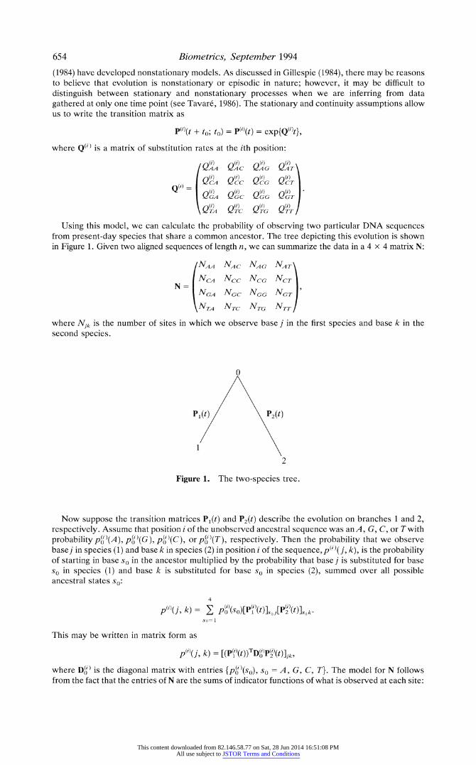
Using this model, we can calculate the probability of observing two particular DNA sequences from present-day species that share a common ancestor. The tree depicting this evolution is shown in Figure 1. Given two aligned sequences of length n, we can summarize the data in a 4 x 4 matrix N:
NAA NA C NAG NAT
ANC NCC NCG NCT N
NGA NGC NGG NGT
NTA NTC NTG NTT
where N/k is the number of sites in which we observe base j in the first species and base k in the second species.
0
P1( )(t)
1
2
Figure 1. The two-species tree.
Now suppose the transition matrices P1(t) and P2(t) describe the evolution on branches 1 and 2, respectively. Assume that position i of the unobserved ancestral sequence was anA, G, C, or Twith probability pg )(A), p(')(G), p(')(C), or p(')(T), respectively. Then the probability that we observe basej in species (1) and base k in species (2) in position i of the sequence,p(')(j, k), is the probability of starting in base so in the ancestor multiplied by the probability that base j is substituted for base so in species (1) and base k is substituted for base so in species (2), summed over all possible ancestral states so:
4 M (j,( k) =Ep)(So)[P(l )(t)l ,,j[P(2i)(t)]stk-
so= I
This may be written in matrix form as
p (i)(,j k) = [(P(i)(t))T-Do P((t)]jk,
where Do) is the diagonal matrix with entries {p(')(so), so = A, G, C, T}. The model for N follows from the fact that the entries of N are the sums of indicator functions of what is observed at each site:
This content downloaded from 82.146.58.77 on Sat, 28 Jun 2014 16:51:08 PMAll use subject to JSTOR Terms and Conditions

A Test for DNA Evolutionaty Models 655
1= Njk = il - k
(1J(k) indicates whether we have a base j in the first species and a base k in the second species at position i in the sequence.) Then the expected value of the observed matrix N is the sum of the expected values over all sites:
E[N]= (p(li)(t))T D(OP(i)(t) . (G) i== 1
We call this model (G), the general model, because it encompasses the models below. This model has a total of 12n + 3n + 12n = 27n parameters to be estimated from the data. The data matrix N, however, has only 15 degrees of freedom. It is thus not possible to estimate the parameters from the data. It is common to decrease the number of parameters estimated by making some simplifying assumptions.
2.1 Common Simplifying Assumptions
I. Positions in the sequence are identically distributed. Most models assume that the rates of evolution for all positions in the sequence are equal:
P(')(t) = Pl(t) for all i = 1, ..., i;
P(2i)(t) = P2(t) for all i = 1, , n;
and D(') = Do for all i = 1,..., n.
Under this assumption, the number of parameters to estimate is reduced to 27.
II. Positions ate independent. This assumption allows us to estimate the parameters via a likelihood method. The test developed in Section 3 utilizes this assumption and Assumption I to conclude that the data matrix N is multinomially distributed.
III. Evolution is reversible. If we assume that the evolutionary process is reversible, then
D(')P(-)(t) = (P(i)(t))TD(i)
where D(i) is the diagonal matrix containing the left eigenvector of P(')(t). This equation puts some constraints on the form of the transition matrix P(')(t); in particular, it reduces the number of parameters in p(i) from 12 to 9.
IV. Process is at equilibrium. If we assume that the evolutionary process is at equilibrium, then at each position i, the ancestral base frequencies will equal the stationary probabilities or, equivalently, the left eigenvector of the transition matrix P(')(t). In other words,
Do) = D(') for all i = 1,..., n.
In this case, the entries of D(i) are determined from the transition matrix P(i)(t) and for each position in the sequence there are three fewer parameters to fit.
2.2 Models The Markov models commonly used can be described by which combination of assumptions they make. Some examples are the following:
A. Assuming (I) and (II), the model for N becomes
BEN] = nP (t)DoP2(t)I (A)
This model has been used by Barry and 1Hartigan (1987) and Tavare and Janzen (unpublished manuscript). These assumptions reduce the number of parameters to 27. Tavare and Janzen also suggested two simpler models that constrain the transition matrices and have only 11 or 15 parameters to estimate.
This content downloaded from 82.146.58.77 on Sat, 28 Jun 2014 16:51:08 PMAll use subject to JSTOR Terms and Conditions
656 Biometrics, September 1994
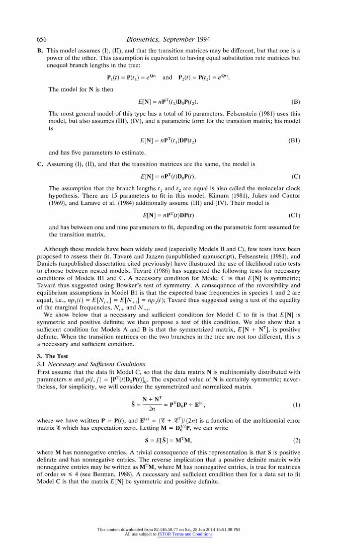
B. This model assumes (I), (II), and that the transition matrices may be different, but that one is a power of the other. This assumption is equivalent to having equal substitution rate matrices but unequal branch lengths in the tree:
Pl(t) = P(tj) = eQt and P2(t) = P(t2) = eQt2.
The model for N is then
E[N] = npT(tl)DOP(t2) (B)
The most general model of this type has a total of 16 parameters. Felsenstein (1981) uses this model, but also assumes (III), (IV), and a parametric form for the transition matrix; his model is
E[N] = npT(tl)DP(t2) (B1)
and has five parameters to estimate.
C. Assuming (I), (II), and that the transition matrices are the same, the model is
E[N] = nPT(t)D,P(t). (C)
The assumption that the branch lengths t1 and t2 are equal is also called the molecular clock hypothesis. There are 15 parameters to fit in this model. Kimura (1981), Jukes and Cantor (1969), and Lanave et al. (1984) additionally assume (III) and (IV). Their model is
E[N] = nPT(t)DP(t) (C1)
and has between one and nine parameters to fit, depending on the parametric form assumed for the transition matrix.
Although these models have been widely used (especially Models B and C), few tests have been proposed to assess their fit. Tavar6 and Janzen (unpublished manuscript), Felsenstein (1981), and Daniels (unpublished dissertation cited previously) have illustrated the use of likelihood ratio tests to choose between nested models. Tavar6 (1986) has suggested the following tests for necessary conditions of Models Bi and C. A necessary condition for Model C is that E [N] is symmetric; Tavar6 thus suggested using Bowker's test of symmetry. A consequence of the reversibility and equilibrium assumptions in Model Bi is that the expected base frequencies in species 1 and 2 are equal, i.e., npl(i) = E[Ni,] = E[N+j] = np2(i); Tavar6 thus suggested using a test of the equality of the marginal frequencies, Ni, and N,j.
We show below that a necessary and sufficient condition for Model C to fit is that E [N] is symmetric and positive definite; we then propose a test of this condition. We also show that a sufficient condition for Models A and B is that the symmetrized matrix, E [N + NT], is positive definite. When the transition matrices on the two branches in the tree are not too different, this is a necessary and sufficient condition.
3. The Test 3.1 Necessary and Sufficient Conditions First assume that the data fit Model C, so that the data matrix N is multinomially distributed with parameters n and p(i, j) = [PT(t)DOP(t)]jj. The expected value of N is certainly symmetric; never- theless, for simplicity, we will consider the symmetrized and normalized matrix
N+ NT g = = pTDOp + E(s), (1) 2n
where we have written P = P(t), and E(s) = (W + WT)/ (2n) is a function of the multinomial error matrix Z which has expectation zero. Letting M = Do/2P, we can write
S = E[S] = MTM, (2)
where M has nonnegative entries. A trivial consequence of this representation is that S is positive definite and has nonnegative entries. The reverse implication that a positive definite matrix with nonnegative entries may be written as MTM, where M has nonnegative entries, is true for matrices of order m S 4 (see Berman, 1988). A necessary and sufficient condition then for a data set to fit Model C is that the matrix E [N] be symmetric and positive definite.
This content downloaded from 82.146.58.77 on Sat, 28 Jun 2014 16:51:08 PMAll use subject to JSTOR Terms and Conditions
A Test for DNA Evolutionary Models 657
Model Cl (and Bi) additionally assumes the evolutionary process is reversible and at equilibrium. These conditions also need to be tested to judge the fit of these models. A consequence of these assumptions in Model Bi is that E [N] = nPT(t1)DP(t2) can be rewritten as
( 2 ( t2)
or as equation (2). The test given below, along with tests of the equilibrium and reversibility assumptions, will then assess the fit of this model.
In Models A and B, E[N] is neither necessarily symmetric nor positive definite; it is, however, positive stable so that all eigenvalues have positive real parts. This follows from the fact that Do, PI, and P2 have all positive real eigenvalues, implying that det(E [N]) > 0, and the fact that tr(E [N]) > 0 (see Horn and Johnson, 1991, p. 94). A sufficient condition for the positive stability of N is the positive definiteness of N + NT (or A) (see Horn and Johnson, 1991, p. 3). We show that this is a necessary and sufficient condition for the fit of Models A and B, when the transition matrices, PI(t) and P2(t), or P(tJ) and P(t2), are not too different.
In Model B, S is positive definite when the branch lengths t, and t2 are similar. Letting h = |t2 - tll, then the branch lengths are similar when only a moderate amount of evolution has occurred in time h or when P(h) is diagonally dominant:
Pii(h) >_ max( Pij(h), EPji(h)) i = l,* , 4- (3)
This is shown in the Appendix. In Model A, S is positive definite as long as the transition matrices PI(t) and P2(t) are similar.
Letting H = P2(t) - Pl(t), the transition matrices are similar when
||DOKJ.1|HH|2 < min A (PT(t)D0P1(t)). (4) A
Here 11H112 is the L2 norm, and lI is the ac-norm. In this case, the test proposed below is appropriate. Again, we leave the proof to the Appendix.
Recall that Model G models the evolution of each position in the sequence with a different transition matrix
E[N] = (P()(t))TD(')P ((t). i= 1
When condition (4) is satisfied for each pair of transition matrices P(')(t) and P(')(t), the symmetrized version of this matrix is positive definite and has nonnegative entries because it is the sum of positive definite matrices with nonnegative entries. The test proposed below, however, may not be appro- priate because the data matrix N is not multinomially distributed, but is a mixture of multinomial random variables. If each position has a different transition matrix
P()(t) X? P(i)(t) for i ? j
describing its evolution through time, the covariance matrix of N is the same as in the other models and the test presented below is appropriate. This is the case in the heterogeneous rate model suggested by Kelly and Rice (in press) when the rates are realizations of a continuous random variable. However, if there are sets of positions evolving according to the same transition matrices, there may be overdispersion or underdispersion which may bias the test statistic (5) suggested in the next section [see McCullagh and Nelder (1989, p. 174) on cluster overdispersion]. For example, in Fitch's (1986) two-state model, some positions do not evolve [i.e., according to the transition matrix PS(t) = I] and the remaining positions evolve according to the matrix P,(t); in this case there will be overdispersion and the variance of the smallest eigenvalue estimated from equation (6) will be an underestimate. The test presented here will then reject too often.
3.2 The Test We now have a test of the fit of many Markov models-a test that the smallest eigenvalue is positive. To develop this test, we need the distribution of this eigenvalue. When the entries of the matrix are Gaussian, this distribution is a well-studied problem (see Srivastava and Khatri, 1979). When the entries are multinomially distributed, however, the problem is not well known. Our test of the
This content downloaded from 82.146.58.77 on Sat, 28 Jun 2014 16:51:08 PMAll use subject to JSTOR Terms and Conditions

658 Biometrics, September 1994
positivity of the smallest eigenvalue of 8, A(S), is based on the asymptotic distribution of this function. A Taylor's series argument for a totally differentiable function of an asymptotically multivariate normal random variable shows that the asymptotic distribution of
n(A(A) - A(S))
is normal with mean zero and variance
o-2(A) = y(2)TSY(2)-A2(S),
where y is the eigenvector of S associated with its smallest eigenvalue, A(S), and y(2) iS the vector with entries y2. The proof is left to the Appendix.
We may now test the hypothesis with the test statistic
T (n A S) '(5) &(A)
where we have approximated o-(A) with
-(A) = (i(2)TAi(2) _ A2()) 1/2, (6)
where x is the eigenvector of A associated with A(S). This statistic is approximately normally distributed since we can write
T n A( o-(A) T=x o-(A) &(A)
The first term in the product converges in distribution to a N(O, 1) random variable and the second term converges in probability to 1. The statistic thus converges to a N(O, 1) random variable. Our test of the positivity of the smallest eigenvalue is then just a z-test using statistic (5).
4. Examples Many published aligned sequences for two species have only a moderate amount of substitutions, so that the summary data matrix N is diagonally dominant. In this case, all eigenvalues are positive and a Markov model will fit the data. For more divergent sequence pairs, the data matrix will not be diagonally dominant and the fit of a Markov model is then in question. Finding highly divergent sequence pairs with the correct alignment, however, is difficult. The alignment problem is somewhat simplified when the sequences are protein coding regions since the sequences occur in triplets. Both examples presented here are of this type.
4.1 Example 1 The first example comes from Brown et al. (1982) mitochondrial DNA sequence data from a gibbon (Hylobates lar) and a chimpanzee (Pan troglodytes). These sequences code for three tRNA's and parts of two proteins. The total length is 896 base pairs; our analysis is of the 232 third position protein-coding sites. Mitochondrial DNA is known to evolve at higher rates than nuclear DNA and third position sites evolve faster than first and second position sites. The third position data are divergent enough so that the data matrix N is not diagonally dominant, yet the first and second position data are less divergent and thus simplify the alignment problem. The data matrix is as follows:
Chimp Gibbon A C G T
A 57 11 6 2
C 7 ~1 1 1
N= 9 3 72 211. \ 4 02512/
If we symmetrize and divide by n, we get our matrix S:
This content downloaded from 82.146.58.77 on Sat, 28 Jun 2014 16:51:08 PMAll use subject to JSTOR Terms and Conditions
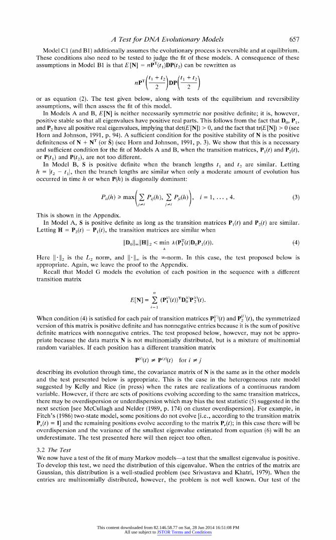
A Test for DNA Evolutionary Models 659
.2457 .0388 .0323 .0129\ j .0388 .0043 .0086 .0022
.0323 .0086 .3103 .0991
.0129 .0022 .0991 .0517
The eigenvalues of A are
A I = .3562, A2 = .2396, A3 = .0181, A4 =-.00185.
For this data set the smallest eigenvalue is negative, but because it is so small it may not be sufficient evidence that the data do not fit a Markov model. The test statistic (5) proposed above is
\/fA4 T = VnA4
- -.363. (k^(2)TA^(2) _
- 2)1/2
The P-value of this statistic for a one-sided test is .3594 and thus we would not reject the null hypothesis that the data fit the model.
A second estimate of the variability of the smallest eigenvalue was calculated from a parametric bootstrap sample, as described in Efron (1982). One hundred samples of the observed data matrix N were simulated in the following way. Since the entries of N are multinomial with probabilities Sij, each sample matrix was generated from this distribution with parameters n and Si,. The sample matrices were then symmetrized and divided by n; in this way we obtained the 100 simulated sample matrices (SU), i = 1, . . , 100). Eigenvalues were calculated for each of these matrices. The statistics on the smallest eigenvalues of the simulated matrices are:
A =-.00397, 6i(A) = .00525.
This bootstrap sample standard deviation agrees very well with the standard deviation of A of .0051 calculated from equation (6).
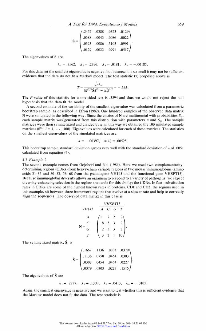
4.2 Example 2 The second example comes from Gojobori and Nei (1984). Here we used two complementarity- determining regions (CDRs) from heavy-chain variable regions in two mouse immunoglobins (amino acids 31-35 and 50-53, 56-68 from the pseudogene VH145 and the functional gene VHSPT15). Because immunoglobin diversity allows an organism to respond to a variety of pathogens, we expect diversity-enhancing selection in the regions that code for this ability: the CDRs. In fact, substitution rates in CDRs are some of the highest known rates in proteins. CD1 and CD2, the regions used in this example, sit between three framework regions that evolve at a slower rate and help to correctly align the sequences. The observed data matrix in this case is
VHSPT1 5
VH145 A C G T
A 11 7 2 2 C 8 5 3 2
N = G 2 3 3 2.
T 3 2 1 10
The symmetrized matrix, S, is
.1667 .1136 .0303 .0379\
.1136 .0758 .0454 .0303
.0303 .0454 .0454 .0227
.0379 .0303 .0227 .1515
The eigenvalues of S are
A1l .2777, A2 = .1309, A3 = .0413, A4 =-.0105.
Again, the smallest eigenvalue is negative and we want to test whether this is sufficient evidence that the Markov model does not fit the data. The test statistic is
This content downloaded from 82.146.58.77 on Sat, 28 Jun 2014 16:51:08 PMAll use subject to JSTOR Terms and Conditions

660 Biometrics, September 1994
nA4 T =
nA, - --.305. (i(2)TS^(2) _ A 2)1/2
The P-value of this statistic for a one-sided test is .3632 and thus we would not reject the null hypothesis that the data fit the model. A bootstrap sample standard deviation was calculated for this example as described in the first example. The statistics on the smallest eigenvalues of 100 simulated matrices are
A = -.0206, 6-(A) = .0324.
The bootstrap estimate again agrees well with the standard deviation calculated from equation (6): for this example &(A) = .0345.
5. Conclusions Here we demonstrate a test to assess whether a general Markov model will fit DNA sequence data from two species. If the species are closely related and the number of nucleotide substitutions is small, a Markov model will fit the data. When the species are more divergent (the average number of substitutions per site is more than .5), the fit of a Markov model may be questioned. The first test is very simple: check that the observed data matrix is diagonally dominant. If it is, a Markov model will fit the data. Otherwise, the eigenvalues must be computed and if one is negative, the test proposed here will indicate whether there is evidence to reject a Markov model. A test that rejects the null hypothesis indicates the following: (1) a Markov model of the type presented here does not fit the data; (2) if Model A or B fits the data, then the difference in transition matrices is too large; (3) if Model G fits the data, then either the transition matrices are too different or there are sets of positions evolving according to the same transition matrices.
A negative eigenvalue that is not large enough to reject a Markov model will still cause problems when estimating evolutionary parameters. Barry and Hartigan's (1987) measure of evolution has been shown to equal k, the average number of substitutions per site, in the Kimura (1981) and Jukes and Cantor (1969) models. This measure is
-4 log(det(fLy1N/n)) = -4 log(det(fDy1) det(N/n)),
where the entries of Do are IjNij/n. If S = (N + NT)/(2n) has a negative eigenvalue, N/n also has a negative eigenvalue (see Horn and Johnson, 1991, p. 3) and then the measure above is undefined. Gillespie (1986) found this problem in analyses of the third position sites in mammalian ae-hemoglo- bin, insulin, cytochrome b, and cytochrome oxidase 1, 2, and 3. Kimura (1981) noted that if all the data sets with negative eigenvalues, or undefined k, are excluded, then k estimated from the remaining data may be seriously underestimated. It is unclear to us how to resolve this problem.
We argue against the blind use of a particular model of molecular evolution. The fit of a model should be assessed before relying on estimated parameters; at least, the consequent biases in using an incorrect model should be understood. Further research is needed in the areas of developing tests of model assumptions and in assessing the biases associated with the incorrect use of models. The testing of assumptions in evolutionary models is important not only to obtain more accurate parameter estimates, but also to increase our understanding of the nature of the evolutionary process.
ACKNOWLEDGEMENTS
I would like to thank John Rice for suggesting the problem of testing Markovian models, showing me Berman's paper, and making many helpful comments. I would also like to thank Choudary Hanu- mara and the referees for their comments.
RESUME
Le modele Markovien d'evolution des sequences d'ADN a bencficie recemment d'un regain d'in- teret car, de par sa nature statistique, il permet de tester nombre d'hypotheses sur l'evolution des especes. Nous proposons ici un test pour determiner si les donnees provenant de deux especes ayant un ancetre commun sont en accord avec un modele Markovien. Nous illustrons ce test avec deux exemples de donnees qui ne semblent pas a priori en accord avec un modele de Markov.
This content downloaded from 82.146.58.77 on Sat, 28 Jun 2014 16:51:08 PMAll use subject to JSTOR Terms and Conditions

A Test for DNA Evolutionary Models 661
REFERENCES
Barry, D. and Hartigan, J. A. (1987). Asynchronous distance between homologous DNA sequences. Biometrics 43, 261-276.
Berman, A. (1988). Complete positivity. LinearAlgebra and Its Applications 107, 57-63. Blaisdell, B. E. (1985). A method of estimating from two aligned present-day DNA sequences their
ancestral composition and subsequent rates of substitution, possibly different in the two lineages, corrected for multiple and parallel substitutions at the same site. Journal of Molecular Evolution 22, 69-81.
Brown, W. M., Prager, E. M., Wang, A., and Wilson, A. C. (1982). Mitochondrial DNA sequences of primates: Tempo and mode of evolution. Jolrnal of Molecular Evolution 18, 225-239.
Efron, B. (1982). The Jackknife, the Bootstrap and Other Resampling Plans. CBMS-NSF Regional Conference Series in Applied Mathematics, Monograph 38. Philadelphia: Society for Industrial and Applied Mathematics.
Felsenstein, J. (1981). Evolutionary trees from DNA sequences: A maximum likelihood approach. Journal of Molecular Evolution 17, 368-376.
Fitch, W. M. (1986). The estimate of total nucleotide substitutions from pairwise differences is biased. Philosophical Transactions of the Royal Society of London, Series B 312, 317-324.
Gillespie, J. H. (1984). The molecular clock may be an episodic clock. Proceedings of the National Academy of Science, U.S.A. 81, 8009-8013.
Gillespie, J. H. (1986). Variability of evolutionary rates of DNA. Genetics 113, 1077-1091. Gojobori, T., Ishii, K., and Nei, M. (1982). Estimation of average number of nucleotide substitu-
tions when the rate of substitution varies with nucleotide. Journal of Molecular Evolution 18, 414-423.
Gojobori, T. and Nei, M. (1984). Concerted evolution of the immunoglobin VH gene family. Molecular Biology and Evolution 1(2), 195-212.
Golding, G. B. (1983). Estimates of DNA and protein sequence divergence: An examination of some assumptions. Molecular Biology and Evolution 1(1), 125-142.
Horn, R. A. and Johnson, C. R. (1991). Topics in MatrixAnalysis. Cambridge: Cambridge Univer- sity Press.
Jukes, T. H. and Cantor, C. R. (1969). Evolution of protein molecules. In Mammalian Protein Metabolism, N. H. Munro (ed.), 21-123. New York: Academic Press.
Kelly, C. and Rice, J. (in press). Modeling nucleotide evolution: A heterogeneous rate analysis. To appear in Mathematical Biosciences.
Kimura, M. (1981). Estimation of evolutionary distances between homologous nucleotide se- quences. Proceedings of the National Academy of Science 78(1), 454-458.
Lanave, C., Preparata, G., Saccone, C., and Serio, G. (1984). A new method for calculating evolutionary substitution rates. Journal of Molecular Evolution 20, 86-93.
Magnus, J. R. (1988). Matrix Differential Calculus with Applications in Statistics and Economics. New York: Wiley.
McCullagh, P. and Nelder, J. A. (1989). Generalized Linear Models. London: Chapman and Hall. Rao, C. R. (1965). Linear Statistical Inference and Its Applications. New York: Wiley. Srivastava, M. S. and Khatri, C. G. (1979). An Introduction to Multivariate Statistics. New York:
Elsevier North-Holland. Stewart, G. W. (1973). Introduction to Matrix Computation. New York, London: Academic Press. Takahata, N. (1991). Overdispersed molecular clock at the major histocompatibility complex loci.
Proceedings of the Royal Society of London, Series B 243, 13-18. Tavare, S. (1986). Some probabilistic and statistical problems in the analysis of DNA sequences.
Lectures on Mathematics in the Life Sciences 17, 57-86.
Received August 1992; revised December 1992 and March 1993; accepted March 1993.
APPENDIX
A.1 Proof of Necessary and Sufficient Conditions for Model B
Model B is equivalent to model (2) when P(h) is diagonally dominant.
Proof: The model for the evolution of two species in this case is
E[N] = npT(t )DOP(t2) = npT(t )DOP(h)P(tl).
The expected value of the symmetrized matrix S is then
S = PT(t )[DOP(h) + PT(h)DO]P(tl),
and assuming that P(h) is diagonally dominant implies that
This content downloaded from 82.146.58.77 on Sat, 28 Jun 2014 16:51:08 PMAll use subject to JSTOR Terms and Conditions
662 Biometrics, September 1994
DH = DOP(h) + pT(h)DO
is also diagonally dominant, which implies that it is positive definite. Since DH also has positive entries, it may be written as yTy by the reverse implication, and thus S = MTM, where M = YP(tj).
A.2 Proof of Necessary and Sufficient Conditions for Model A
Model A is equivalent to model (2) when the L2 norm of H = P2(t) - P1(t) is less than
min A((P1(t))T DOP1(t)) A
Proof: The expected value of the symmetrized matrix S for Model A is
E[S] = I{PT(t)DOP2(t) + PT(t)DOPj(t)}.
For convenience we will use the shorthand notation, P = P1(t). Then using the expression P2(t) = P1(t) + H, we obtain
E[S] = {PTDoP + PTDOH + PTDOP + HTDOP}
PTDOP + 1 {PTDOH + HTDOP}.
We write this as
B + B T E[S] = A + 2
where both A and (B + BT)/2
are Hermitian. A lower bound for the smallest eigenvalue of E [S]
is the sum of the smallest eigenvalues of A and (B + BT)/2 [see, for example, Stewart (1973, p. 315)]:
B + B T A1(E[S]) > A1(A) + A( 2B)
Now
A1( B) 'J IlB + B 112 <
IIBI12
< |lPT 121lDOl21HIl2
S max [DO]jLjHHI2
= JIDOfl.HIH2-
This implies that
A (E[S]) > 0
when A1(PTDoP) J JDollo,JHJl12.
A.3 Proof of the Distribution of the Smallest Eigenvalue
Consider the data matrix N., and the symmetrized matrix S,1 to be functions of the length n of the DNA sequence. Since N,, is multinomially distributed, with parameters n and Sij, we obtain that 6/N/n = V/(N,,/n - S) is asymptotically multivariate normal with mean zero and variance
COy (-, k1) =1 \ni 'k \z n] ki
ad =
I ~~otherwise.
Since CtS = (t + ctT)/ (2n), V'WCf) = V'(S,1 - 5) is also asymptotically multivariate normal with mean zero, but with variance V:
This content downloaded from 82.146.58.77 on Sat, 28 Jun 2014 16:51:08 PMAll use subject to JSTOR Terms and Conditions
A Test for DNA Evolutionary Models 663
Vi kl C cov(CnKS) C(s)) = cov 'kl +
1 ij kl- \ ij Ik- i ji Wkl i ji tIk i = 4 (cov( , i/?' + covt/ZS ?/?? + cov , ?) + cov\(Z, ?/?i)
Sii(l - Sii) if i =1 = k = 1,
= 2n - n if (i, j) = (k, 1) or (i, j) = (1, k) 2n n
otherwise. n
The function A(S,,) that computes the smallest eigenvalue of S,, is totally differentiable with respect to the entries of S,. A Taylor's series argument (see Rao, 1965) then gives that the asymptotic distribution of
n(A(S) - A(S))
is normal with mean zero and variance
4 aAA(S) OA(S) nr 2(A(S)) =n Z 'ijkl (7
ij, k,1= 1 a iy
a kl
It is left only to compute the derivative of the smallest cigenvalue of a matrix S with respect to its entries (cf. Magnus, 1988). Let y be the eigenvector associated with the smallest eigenvalue A; then since S is symmetric we have Sy = Ay and YTS = YTA. Now yTy = 1 implies that
ay_T ay ayT y + yT - = 2 y = O. os.. as.. as..
We then have
aA a T(Ay) ayT = (YTAY) yT +A Y as. as.. as. as.
T (Ay) =T a(Sy) as.. asY .
aS T ay =y y + Y
aS-1, + AyT
as__
=yT _ y =yiyj
The variance in equation (7) now becomes
4
no 2(A (S)) = E nVijklyyjYjYkY i,j, k, l=1
4 4 4
E y4S (i1 - Sii) + E y72yj2Sij(l - 2Sij) - Yk, 1= Y
1;15 i==1 ~ x (i, j,Xk,lI)
4 4
= E y72y7511 - E YiY1YkY/5i1Sk/* i,j==1 i,j,k,l=1
This content downloaded from 82.146.58.77 on Sat, 28 Jun 2014 16:51:08 PMAll use subject to JSTOR Terms and Conditions

664 Biometrics, September 1994
Letting y(2) denote the vector with entries y(2) = y2, we have = y(2)TSy(2) _ (YTSY)2
= y(2)TSy(2) _ A2.
This content downloaded from 82.146.58.77 on Sat, 28 Jun 2014 16:51:08 PMAll use subject to JSTOR Terms and Conditions