A Temporal Trace Language for Modelling Real World Phenomenon
35
A Temporal Trace Language for Formal Modelling and Analysis of Agent Systems Alexei Sharpanskykh and Jan Treur Abstract This chapter presents the hybrid Temporal Trace Language (TTL) for for- mal specification and analysis of dynamic properties of multi-agent systems. This language supports specification of both qualitative and quantitative aspects, and sub- sumes languages based on differential equations and temporal logics. TTL has a high expressivity and normal forms that enable automated analysis. Software en- vironments for performing verification of TTL specifications have been developed. TTL proved its value in a number of domains. 1 Introduction Traditionally, the multi-agent paradigm has been used to improve efficiency of soft- ware computation. Languages used to specify such multi-agent systems often had limited expressive power (e.g., executable, close to (logic) programming languages), which nevertheless was sufficient to describe complex distributed algorithms. Re- cently many agent-based methods, techniques and methodologies have been devel- oped to model and analyse phenomena in the real world (e.g., social, biological, and psychological structures and processes). By formally grounded multi-agent system modelling one can gain better understanding of complex real world processes, test existing theories from natural and human sciences, identify different types of prob- lems in real systems. Modelling dynamics of systems from the real world is not a trivial task. Cur- rently, continuous modelling techniques based on differential and difference equa- Alexei Sharpanskykh Vrije Universiteit Amsterdam, Department of Artificial Intelligence De Boelelaan 1081a, 1081 HV Amsterdam, The Netherlands e-mail: [email protected] Jan Treur Vrije Universiteit Amsterdam, Department of Artificial Intelligence De Boelelaan 1081a, 1081 HV Amsterdam, The Netherlands e-mail: [email protected] 1
-
Upload
bilal-javed -
Category
Documents
-
view
229 -
download
0
description
The document describes use of TTL to create and simulate real world models using computational power.
Transcript of A Temporal Trace Language for Modelling Real World Phenomenon
A Temporal Trace Language forFormal Modelling and Analysis ofAgent Systems
Alexei Sharpanskykh and Jan Treur
Abstract This chapter presents the hybrid Temporal Trace Language (TTL) for for-mal specification and analysis of dynamic properties of multi-agent systems. Thislanguage supports specification of both qualitative and quantitative aspects, and sub-sumes languages based on differential equations and temporal logics. TTL has ahigh expressivity and normal forms that enable automated analysis. Software en-vironments for performing verification of TTL specifications have been developed.TTL proved its value in a number of domains.
1 Introduction
Traditionally, the multi-agent paradigm has been used to improve efficiency of soft-ware computation. Languages used to specify such multi-agent systems often hadlimited expressive power (e.g., executable, close to (logic) programming languages),which nevertheless was sufficient to describe complex distributed algorithms. Re-cently many agent-based methods, techniques and methodologies have been devel-oped to model and analyse phenomena in the real world (e.g., social, biological, andpsychological structures and processes). By formally grounded multi-agent systemmodelling one can gain better understanding of complex real world processes, testexisting theories from natural and human sciences, identify different types of prob-lems in real systems.
Modelling dynamics of systems from the real world is not a trivial task. Cur-rently, continuous modelling techniques based on differential and difference equa-
Alexei SharpanskykhVrije Universiteit Amsterdam, Department of Artificial Intelligence De Boelelaan 1081a, 1081 HVAmsterdam, The Netherlands e-mail: [email protected]
Jan TreurVrije Universiteit Amsterdam, Department of Artificial Intelligence De Boelelaan 1081a, 1081 HVAmsterdam, The Netherlands e-mail: [email protected]
1

2 Alexei Sharpanskykh and Jan Treur
tions are often used in natural science to address this challenge, with limited success.In particular, for creating realistic continuous models for natural processes a greatnumber of equations with a multitude of parameters are required. Such models aredifficult to analyze, both mathematically and computationally. Further, continuousmodelling approaches, such as the Dynamical Systems Theory [32], provide littlehelp for specifying global requirements on a system being modelled and for defininghigh level system properties that often have a qualitative character (e.g., reasoning,coordination). Also, sometimes system components (e.g., switches, thresholds) havebehaviour that is best modelled by discrete transitions. Thus, the continuous mod-elling techniques have limitations, which can compromise the feasibility of systemmodelling in different domains.
Logic-based methods have proved useful for formal qualitative modelling of pro-cesses at a high level of abstraction. For example, variants of modal temporal logic[3, 17] gained popularity in agent technology, and for modelling social phenomena.However, logic-based methods typically lack quantitative expressivity essential formodelling precise timing relations as needed in, e.g., biological and chemical pro-cesses.
Furthermore, many real world systems (e.g., a television set, a human organisa-tion, a human brain) are hybrid in nature, i.e., are characterized by both qualitativeand quantitative aspects. To represent and reason about structures and dynamics ofsuch systems, the possibility of expressing both qualitative and quantitative aspectsis required. Moreover, to tackle the issue of complexity and scalability the possibil-ity of modelling of a system at different aggregation levels is in demand. In this casemodelling languages should be able to express logical relationships between partsof a system.
To address the discussed modelling demands, the Temporal Trace Language(TTL) is proposed, which subsumes languages based on differential equations andtemporal logics, and supports the specification of the system behaviour at differentlevels of abstraction.
Generally, the expressivity of modelling languages is limited by the possibility toperform effective and efficient analysis of models. Analysis techniques for complexsystems include simulation based on system models, and verification of dynamicproperties on model specifications and traces generated by simulation or obtainedempirically.
For simulation it is essential to have limitations to the language. To this end,an executable language that allows specifying only direct temporal relations can bedefined as a sublanguage of TTL; cf. [8]. This language allows representing thedynamics of a system by a (possible large) number of simple temporal (or causal)relations, involving both qualitative and quantitative aspects. Furthermore, usinga dedicated tool, TTL formulae that describe the complex dynamics of a systemspecified in a certain format may be automatically translated into the executableform. Based on the operational semantics and the proof theory of the executablelanguage, a dedicated tool has been developed that allows performing simulationsof executable specifications.
A Temporal Trace Language for Formal Modelling and Analysis of Agent Systems 3
To verify properties against specifications of models two types of analysis tech-niques are widely used: logical proof procedures and model checking [10]. Bymeans of model checking entailment relations are justified by checking propertieson the set of all theoretically possible traces generated by execution of a systemmodel. To make such verification feasible, expressivity of both the language usedfor the model specification and the language used for expressing properties has tobe sacrificed to a large extent. Therefore, model specification languages provided bymost model checkers allow expressing only simple temporal relations in the form oftransition rules with limited expressiveness (e.g., no quantifiers). For specifying acomplex temporal relation a large quantity (including auxiliary) of interrelated tran-sition rules is needed. In this chapter normal forms and a transformation procedureare introduced, which enable automatic translation of an expressive TTL specifica-tion into the executable format required for automated verification (e.g., by modelchecking). Furthermore, abstraction of executable specifications, as a way of gener-ating properties of higher aggregation levels, is considered in this chapter. In partic-ular, an approach that allows automatic generation of a behavioural specification ofan agent from a cognitive process model is described.
In some situations it is required to check properties only on a limited set of tracesobtained empirically or by simulation (in contrast to model checking which requiresexhaustive inspection of all possible traces). Such type of analysis, which is compu-tationally much cheaper than model checking, is described in this chapter.
The chapter is organised as follows. Section 2 describes the syntax of the TTLlanguage. The semantics of the TTL language is described in Section 3. Multi-levelmodelling of multi-agent systems in TTL and a running example used through-out the chapter are described in Section 4. In Section 5 relations of TTL to otherwell-known formalisms are discussed. In Section 6 normal forms and transforma-tion procedures for automatic translation of a TTL specification into the executableformat are introduced. Furthermore, abstraction of executable specifications is con-sidered in Section 6. Verification of specifications of multi-agent systems in TTL isconsidered in Section 7. Finally, Section 8 concludes the chapter.
2 Syntax of TTL
The language TTL is a variant of an order-sorted predicate logic [24]. Whereas stan-dard multi-sorted predicate logic is meant to represent static properties, TTL is anextension of such language with explicit facilities to represent dynamic propertiesof systems. To specify state properties for system components, ontologies are usedwhich are specified by a number of sorts, sorted constants, variables, functions andpredicates (i.e., a signature). State properties are specified based on such ontologyusing a standard multi-sorted first-order predicate language. For every system com-ponent A (e.g., agent, group of agents, environment) a number of ontologies can bedistinguished used to specify state properties of different types. That is, the ontolo-gies IntOnt(A), InOnt(A), OutOnt(A), and ExtOnt(A) are used to express respec-

4 Alexei Sharpanskykh and Jan Treur
tively internal, input, output and external state properties of the component A. Forexample, a state property expressed as a predicate pain may belong to IntOnt(A),whereas the atom has temperature(environment,7) may belong to ExtOnt(A). Of-ten in agent-based modelling input ontologies contain elements for describing per-ceptions of an agent from the external world (e.g, observed(a) means that a com-ponent has an observation of state property a), whereas output ontologies describeactions and communications of agents (e.g., per f orming action(b) represents ac-tion b performed by a component in its environment).
To express dynamic properties, TTL includes special sorts: T IME (a set of lin-early ordered time points), STATE (a set of all state names of a system), T RACE(a set of all trace names; a trace or a trajectory can be thought of as a timeline witha state for each time point), STATPROP (a set of all state property names), andVALUE (an ordered set of numbers). Furthermore, for every sort S from the statelanguage the following TTL sorts exist: the sort SVARS, which contains all variablenames of sort S, the sort SGTERMS, which contains names of all ground terms, con-structed using sort S; sorts SGT ERMS and SVARS are subsorts of sort STERMS.
In TTL, formulae of the state language are used as objects. To provide names ofobject language formulae ϕ in TTL, the operator (*) is used (written as ϕ ∗), whichmaps variable sets, term sets and formula sets of the state language to the elementsof sorts SGTERMS, STERMS, SVARS and STATPROP in the following way:
1. Each constant symbol c from the state sort S is mapped to the constant name c ′of sort SGTERMS.
2. Each variable x : S from the state language is mapped to the constant name x ′ ∈SVARS.
3. Each function symbol f : S1 × S2 × ...× Sn → Sn+1 from the state language ismapped to the function name f ′ : STERMS
1 ×STERMS2 × ...×STERMS
n → ST ERMSn+1 .
4. Each predicate symbol P : S1 × S2 × ...× Sn is mapped to the function nameP ′ : STERMS
1 ×STERMS2 × ...×STERMS
n → STATPROP.5. The mappings for state formulae are defined as follows:
a. (¬ϕ )∗ = not(ϕ ∗)b. (ϕ &ψ)∗ = ϕ ∗ ∧ψ∗,(ϕ |ψ)∗ = ψ∗ ∨ψ∗c. (ϕ ⇒ ψ)∗ = ϕ ∗ → ψ∗,(ϕ ⇔ ψ)∗ = ϕ ∗ ↔ ψ∗d. (∀x ϕ (x))∗ = ∀x ′ ϕ ∗(x ′), where x is variable over sort S and x ′ is any constant
of SVARS; the same for ∃.
It is assumed that the state language and the TTL define disjoint sets of expres-sions. Therefore, further in TTL formulae we shall use the same notations for theelements of the object language and for their names in the TTL without introducingany ambiguity. Moreover we shall use t with subscripts and superscripts for vari-ables of the sort TIME; and γ with subscripts and superscripts for variables of thesort T RACE.
A state is described by a function symbol state : T RACE ×T IME → STATE. Atrace is a temporally ordered sequence of states. A time frame is assumed to be fixed,linearly ordered, for example, the natural or real numbers. Such an interpretation ofa trace contrasts to Mazurkiewicz traces [26] that are frequently used for analysing
A Temporal Trace Language for Formal Modelling and Analysis of Agent Systems 5
behaviour of Petri nets. Mazurkiewicz traces represent restricted partial orders overalgebraic structures with a trace equivalence relation. Furthermore, as opposed tosome interpretations of traces in the area of software engineering, a formal logicallanguage is used here to specify properties of traces.
The set of function symbols of TTL includes ∨, ∧, →, ↔: STATPROP×STATPROP → STATPROP ; not : STATPROP → STATPROP, and ∀,∃ : SVARS ×STATPROP → STATPROP, of which the counterparts in the state language areboolean propositional connectives and quantifiers. Further we shall use ∨,∧,→,↔in infix notation and ∀,∃ in prefix notation for better readability. For example, usingsuch function symbols the state property about external world expressing that thereis no rain and no clouds can be specified as: not(rain)∧not(clouds).
To formalise relations between sorts VALUE and T IME, functional symbols −,+, /, • : T IME ×VALUE → T IME are introduced. Furthermore, for arithmeti-cal operations on the sort VALUE the corresponding arithmetical functions are in-cluded.
States are related to state properties via the satisfaction relation denoted bythe prefix predicate holds (or by the infix predicate |=): holds(state(γ, t), p) (orstate(γ,t) |= p), which denotes that state property p holds in trace γ at time point t.
Both state(γ,t) and p are terms of the TTL language. In general, TTL terms areconstructed by induction in a standard way from variables, constants and functionsymbols typed with all before-mentioned TTL sorts. Transition relations betweenstates are described by dynamic properties, which are expressed by TTL-formulae.The set of atomic TTL-formulae is defined as:
1. If v1 is a term of sort STATE, and u1 is a term of the sort STATPROP, thenholds(v1,u1) is an atomic TTL formula.
2. If τ1, τ2 are terms of any TTL sort, then τ1 = τ2 is a TTL-atom.3. If t1, t2 are terms of sort T IME, then t1 < t2 is a TTL-atom.4. If v1, v2 are terms of sort VALUE, then v1 < v2 is a TTL-atom.
The set of well-formed TTL-formulae is defined inductively in a standard wayusing Boolean connectives and quantifiers over variables of TTL sorts. An exampleof the TTL formula, which describes observational belief creation of an agent, isgiven below:
In any trace, if at any point in time t1 the agent A observes that it is raining,then there exists a point in time t2 after t1 such that at t2 in the trace the agentA believes that it is raining.
∀γ ∀t1 [holds(state(γ,t1),observation result(itsraining))⇒∃t2 > t1 holds(state(γ,t2),belie f (itsraining))]
The possibility to specify arithmetical operations in TTL allows modelling ofcontinuous systems, which behaviour is usually described by differential equa-tions. Such systems can be expressed in TTL either using discrete or dense timeframes. For the discrete case, methods of numerical analysis that approximate acontinuous model by a discrete one are often used, e.g., Euler’s and Runge-Kutta
6 Alexei Sharpanskykh and Jan Treur
methods [29]. For example, by applying Euler’s method for solving a differentialequation dy/dt = f (y) with the initial condition y(t0) = y0, a difference equationyi+1 = yi + h ∗ f (yi) (with i the step number and h > 0 the step size) is obtained.This equation can be modelled in TTL in the following way:
∀γ ∀t ∀v : VALUE holds(state(γ, t), has value(y,v)) ⇒holds(state(γ,t + 1), has value(y,v+ h• f (v)))
The traces γ satisfying the above dynamic property are the solutions of the dif-ference equation.
Furthermore, a dense time frame can be used to express differential equationswith derivatives specified using the epsilon-delta definition of a limit, which is ex-pressible in TTL. To this end, the following relation is introduced, expressing thatx = dy/dt:
is diff of(γ,x,y) :∀t,w ∀ε > 0 ∃δ > 0 ∀t ′,v,v′0 < dist(t ′,t) < δ & holds(state(γ, t),has value(x,w))&holds(state(γ,t),has value(y,v))&holds(state(γ,t ′),has value(y,v′))⇒ dist((v′ − v)/(t ′ − t),w) < εwhere dist(u,v) is defined as the absolute value of the difference.
Furthermore, a study has been performed in which a number of properties ofcontinuous systems and theorems of calculus were formalized in TTL and used inreasoning [9].
3 Semantics of TTL
An interpretation of a TTL formula is based on the standard interpretation of anorder sorted predicate logic formula and is defined by a mapping I that associateseach:
1. sort symbol S to a certain set (subdomain) DS, such that if S ⊆ S′ then DS ⊆ D′S
2. constant c of sort S to some element of DS
3. function symbol f of type < X1, ...,Xi > → Xi+1 to a mapping: I(X1)× ...×I(Xi) → I(Xi+1)
4. predicate symbol P of type < X1, ...,Xi > to a relation on I(X1)× ...× I(Xi)
A model M for the TTL is a pair M =< I,V >, where I is an interpretationfunction, and V is a variable assignment, mapping each variable x of any sort S toan element of DS. We write V [x/v] for the assignment that maps variables y otherthan x to V (y) and maps x to v. Analogously, we write M[x/v] =< I,V [x/v] >.
A Temporal Trace Language for Formal Modelling and Analysis of Agent Systems 7
If M =< I,V > is a model of the TTL, then the interpretation of a TTL term τ ,denoted by τ M , is inductively defined by:
1. (x)M = V (x), where x is a variable over one of the TTL sorts.2. (c)M = I(c), where c is a constant of one of the TTL sorts.3. f (τ1, ...,τk)M = I( f )(τ M
1 , ...,τ Mk ), where f is a TTL function of type S1 × ...×
Sn → S and τ1, ...,τn are terms of TTL sorts S1, ...,Sn.
The truth definition of TTL for the model M =< I,V > is inductively defined by:
1. |=M Pi(τ1, ...,τk) iff I(Pi)(τ M1 , ...,τ M
k ) = true2. |=M ¬ϕ iff |=M ϕ3. |=M ϕ ∧ψ iff |=M ϕ and iff |=M ψ4. |=M ∀x(ϕ (x)) iff |=M[x/v] ϕ (x) for all v ∈ DS, where x is a variable of sort S.
The semantics of connectives and quantifiers is defined in the standard way. Anumber of important properties of TTL are formulated in form of axioms:
1. Equality of traces:∀γ1,γ2 [∀t[state(γ1,t) = state(γ2, t)] ⇒ γ1 = γ2]
2. Equality of states:∀s1,s2[∀a : STATPROP[truth value(s1,a) = truth value(s2,a)] ⇒ s1 = s2]
3. Truth value in a state:holds(s, p) ⇔ truth value(s, p) = true
4. State consistency axiom:∀γ,t, p (holds(state(γ,t), p) ⇒¬holds(state(γ, t),not(p)))
5. State property semantics:
a. holds(s,(p1∧ p2))⇔ holds(s, p1) & holds(s, p2)b. holds(s,(p1∨ p2))⇔ holds(s, p1) | holds(s, p2)c. holds(s,not(p1)) ⇔¬holds(s, p1)
6. For any constant variable name x from the sort SVARS:holds(s,(∃(x,F))) ⇔∃x′ : SGTERMS holds(s,G), and holds(s,(∀(x,F))) ⇔∀x′ :SGTERMS holds(s,G) with G, F terms of sort STATPROP, where G is obtainedfrom F by substituting all occurrences of x by x ′.
7. Partial order axioms for the sort TIME:
a. ∀t t ≤ t (Reflexivity)b. ∀t1,t2 [t1 ≤ t2 ∧ t2 ≤ t1] ⇒ t1 = t2 (Anti-Symmetry)c. ∀t1,t2,t3 [t1 ≤ t2 ∧ t2 ≤ t3] ⇒ t1 ≤ t3 (Transitivity)
8. Axioms for the sort VALUE: the same as for the sort TIME and standard arith-metic axioms.
9. Axioms, which relate the sorts TIME and VALUE:
a. (t + v1)+ v2 = t +(v1 + v2)b. (t • v1)• v2 = t • (v1 • v2)
8 Alexei Sharpanskykh and Jan Treur
10. (Optional) Finite variability property (for any trace γ).This property ensures that a trace is divided into intervals such that the overallsystem state is stable within each interval, i.e., each state property changes itstruth value at most a finite number of times:∀t0,t1 t0 < t1 ⇒∃δ > 0[∀t[t0 ≤ t & t ≤ t1] ⇒ ∃t2[t2 ≤ t & t < t2 +δ & ∀t3[t2 ≤t3 & t3 ≤ t2 +δ]] ⇒ state(γ, t3) = state(γ, t)]
4 Multi-level Modelling of Multi-Agent Systems in TTL
With increase of the number of elements within a multi-agent system, the complex-ity of the dynamics of the system grows considerably. To analyze the behaviour of acomplex multi-agent system (e.g., for critical domains such as air traffic control andhealth care), appropriate approaches for handling the dynamics of the multi-agentsystem are important. Two of such approaches for TTL specifications of multi-agentsystems are considered in this section: aggregation by agent clustering is consideredin Section 4.1 and organisation structures are discussed in Section 4.2.
4.1 Aggregation by agent clustering
One of the approaches to manage complex dynamics is by distinguishing differentaggregation levels, based on clustering of a multi-agent system into parts or compo-nents with further specification of their dynamics and relations between them; e.g.,[21]. At the lowest aggregation level a component is an agent or an environmentalobject (e.g., a database), with which agents interact. Further, at higher aggregationlevels a component has the form of either a group of agents or a multi-agent systemas a whole. In the simplest case two levels can be distinguished: the lower level atwhich agents interact and the higher level, where the whole multi-agent system isconsidered as one component. In the general case the number of aggregation lev-els is not restricted. Components interact with each other and the environment viainput and output interfaces described in terms of interaction (i.e., input and output)ontologies. A component receives information at its input interface in the form ofobservation results and communication from other components. A component gen-erates at its output communication, observation requests and actions performed inthe environment. Some elements from the agent’s interaction ontology are providedin Table 1.
For the explicit indication of an aspect of a state for a component, to which astate property is related, sorts ASPECT COMPONENT (a set of the componentaspects of a system; i.e., input, output, internal); COMPONENT (a set of all com-ponent names of a system); COMPONENT STATE ASPECT (a set of all namesof aspects of all component states) and a function symbol
A Temporal Trace Language for Formal Modelling and Analysis of Agent Systems 9
Table 1 Interaction ontology
Ontology element Description
observation request f rom f or(C :COMPONENT, I : INFO ELEMENT )
I is to be observed in the world for C (ac-tive observation)
observation result to f or(C :COMPONENT, I : INFO ELEMENT )
Observation result I is provided to C (foractive observation)
observed(I : INFO ELEMENT ) I is observed at the component’s input(passive observation)
communicated f rom to(C1 : COMPONENT,C2 : COMPONENT, s act : SPEECH ACT,I : INFO ELEMENT )
Specifies speech act s act (e.g., inform,request, ask) from C1 to C2 with the con-tent I
to be per f ormed(A : ACT ION) Action A is to be performed
comp aspect : ASPECT COMPONENT ×COMPONENT →COMPONENT STATE ASPECT
are used. In multi-agent system specifications, in which the indication of the com-ponent’s aspects is needed, the definition of the function symbol state introducedearlier is extended as state : TRACE×TIME×COMPONENT STATE ASPECT →STATE. For example,
holds(state(trace1,t1, input(A)),observation result(sunny weather))
Here input(A) belongs to sort COMPONENT STATE ASPECT .At every aggregation level the behaviour of a component is described by a set ofdynamic properties. The dynamic properties of components of a higher aggregationlevel may have the form of a few temporal expressions of high complexity. At alower aggregation level a system is described in terms of more basic steps. Thisusually takes the form of a specification consisting of a large number of temporalexpressions in a simpler format. Furthermore, the dynamic properties of a compo-nent of a higher aggregation level can be logically related by an interlevel relationto dynamic properties of components of an adjacent lower aggregation level. Thisinterlevel relation takes the form that a number of properties of the lower level logi-cally entail the properties of the higher level component.
In the following a running example used throughout the chapter is introduced toillustrate aggregation by agent clustering in a multi-agent system for co-operativeinformation gathering. For simplicity, this system is considered at two aggregationlevels (see Figure 1). At the higher level the multi-agent system as a whole is con-sidered. At the lower level four components and their interactions are specified: twoinformation gathering agents A and B, agent C, and environment component E rep-resenting the external world. Each of the agents is able to acquire partial informationfrom an external source (component E) by initiated observations. Each agent can bereactive or proactive with respect to the information acquisition process. An agentis proactive if it is able to start information acquisition independently of requests ofany other agents, and an agent is reactive if it requires a request from some otheragent to perform information acquisition.

10 Alexei Sharpanskykh and Jan Treur
B E
C
A
Fig. 1 The co-operative information gathering multi-agent system. A and B represent informationgathering agents; C is an agent that obtains the conclusion information; E is an environmentalcomponent.
Observations of any agent taken separately are insufficient to draw conclusionsof a desired type; however, the combined information of both agents is sufficient.Therefore, the agents need to co-operate to be able to draw conclusions. Each agentcan be proactive with respect to the conclusion generation, i.e., after receiving bothobservation results an agent is capable to generate and communicate a conclusionto agent C. Moreover, an agent can be request pro-active to ask information fromanother agent, and an agent can be pro-active or reactive in provision of (alreadyacquired) information to the other agent.
For the lower-level components of the multi-agent system, a number of dynamicproperties were identified and formalized as it is shown below. In the formaliza-tion the variables A1 and A2 are defined over the sort AGENT T ERMS, the constantE belongs to the sort ENVIRONMENTAL COMPONENT GT ERMS, the variable ICis defined over the sort INFORMATION CHUNKT ERMS, the constants IC1, IC2and IC3 belong to the sort INFORMATION CHUNK GT ERMS and the constant Cbelongs to the sort AGENT TERMS.
DP1(A1, A2) (Effectiveness of information request transfer between agents)If agent A1 communicates a request for an information chunk to agent A2 at anytime point t1, then this request will be received by agent A2 at time point t1+ c.∀IC∀t1 [holds(state(γ,t1,out put(A1)),communicated f rom to(A1,A2,request, IC)))
⇒ holds(state(γ,t1+c, input(A2)),communicated f rom to(A1,A2,request, IC))]
DP2(A1, A2) (Effectiveness of information transfer between agents)If agent A1 communicates information chunk to agent A2 at any time point t1, thenthis information will be received by agent A2 at the time point t1+ c.∀IC∀t1 [holds(state(γ,t1,out put(A1)),communicated f rom to(A1,A2, in f orm, IC)))
⇒ holds(state(γ,t1+c, input(A2)),communicated f rom to(A1,A2, in f orm, IC)))]
DP3(A1, E) (Effectiveness of information transfer between an agent and envi-ronment)

A Temporal Trace Language for Formal Modelling and Analysis of Agent Systems 11
If agent A1 communicates an observation request to the environment at any timepoint t1, then this request will be received by the environment at the time pointt1+ c.∀IC∀t1 [holds(state(γ,t1,out put(A1)),observation request f rom f or(A1, IC))
⇒ holds(state(γ,t1+ c, input(E)),observation request f rom f or(A1, IC))]
DP4(A1, E) (Information provision effectiveness)If the environment receives an observation request from agent A1 at any time pointt1, then the environment will generate a result for this request at the time pointt1+ c.∀IC∀t1[holds(state(γ,t1, input(E)),observation request f rom f or(A1, IC))
⇒ holds(state(γ,t1+ c,out put(E)),observation result to f or(A1, IC))]
DP5(E, A1) (Effectiveness of information transfer between environment and anagent)If the environment generates a result for an agent’s information request at any timepoint t1, then this result will be received by the agent at the time point t1+ c.∀IC∀t1[holds(state(γ,t1,out put(E)),observation result to f or(A1, IC))
⇒ holds(state(γ,t1+ c, input(A1)),observation result to f or(A1, IC))]
DP6(A1, A2) (Information acquisition reactiveness)If agent A2 receives a request for an information chunk from agent A1 at any timepoint t1, then agent A2 will generate a request for this information to the environ-ment at the time point t1+ c.∀IC∀t1[holds(state(γ,t1, input(A2)),communicated f rom to(A1,A2,request, IC))
⇒ holds(state(γ,t1+ c,out put(A2)),observation result to f or(A2, IC))]
DP7(A1, A2) (Information provision reactiveness)If exists a time point t1 when agent A2 received a request for a chunk of informationfrom agent A1, then for all time points t2 when the requested information is providedto agent A2, this information will be further provided by agent A2 to agent A1 at thetime point t2+ c.∀IC[∃t1[t1 < t & holds(state(γ, t1, input(A2)),
communicated f rom to(A1,A2,request, IC))]]⇒ ∀t2[t < t2&holds(state(γ, t2, input(A2)),observation result to f or(A2, IC))⇒holds(state(γ,t2+c,out put(A2)),communicated f rom to(A2,A1, in f orm, IC))]]
DP8(A1, A2) (Conclusion proactiveness)For any time points t1 and t2, if agent A1 receives a result for its observation requestfrom the environment (information chunk IC1) at t1 and it receives information re-quired for the conclusion generation from agent A2 (information chunk IC2) at t2,then agent A1 will generate a conclusion based on the received information (infor-mation chunk IC3) to agent C at a time point t4 later than t1 and t2.∀t1,t2 t1 < t & t2 < t&
holds(state(γ,t1, input(A1)),observation result to f or(A1, IC1))&

12 Alexei Sharpanskykh and Jan Treur
holds(state(γ,t2, input(A1)),communicated f rom to(A2,A1, in f orm, IC2))⇒∃ t4 > t&[holds(state(γ,t4,out put(A1)),communicated f rom to(A1,C, in f orm, IC3))]
DP9(A1, E) (Information acquisition proactiveness)At some time point an observation request for information chunk IC1 is generatedby agent A1 to the environment.holds(state(γ,c,out put(A1)),observation request f rom f or(A1, IC1))
DP10(A1, A2) (Information request proactiveness)At some time point a request for information chunk IC2 is communicated by agentA1 to agent A2.holds(state(γ,c,out put(A1)),communicated f rom to(A1,A2,request, IC2))
4.2 Organisation structures
Organisations have proven to be a useful paradigm for analyzing and designingmulti-agent systems [14, 13]. Representation of a multi-agent system as an organ-isation consisting of roles and groups can tackle major drawbacks concerned withtraditional multi-agent models; e.g., high complexity and poor predictability of dy-namics in a system [14]. We adopt a generic representation of organisations, ab-stracted from instances of real agents. As has been shown in [19], organisationalstructure can be used to limit the scope of interactions between agents, reduce orexplicitly increase redundancy of a system, or formalize high-level system goals,of which a single agent may be not aware. Moreover, organisational research hasrecognized the advantages of agent-based models; e.g., for analysis of structure anddynamics of real organisations.
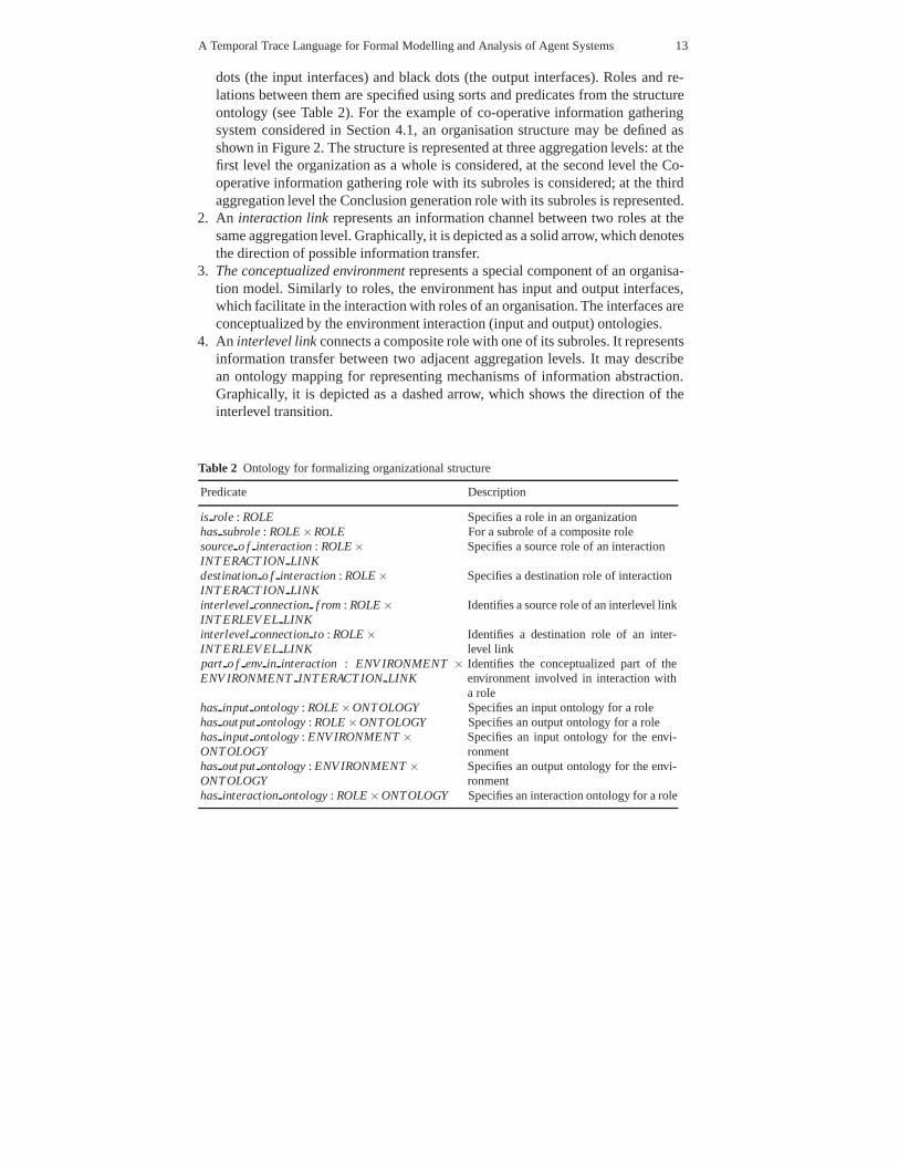
An organisation structure is described by relationships between roles at the sameand at adjoining aggregation levels and between parts of the conceptualized envi-ronment and roles. The specification of an organisation structure uses the followingelements:
1. A role represents a subset of functionalities, performed by an organisation, ab-stracted from specific agents who fulfil them.Each role can be composed by several other roles, until the necessary detailedlevel of aggregation is achieved, where a role that is composed of (interacting)subroles, is called a composite role. Each role has an input and an output inter-face, which facilitate in the interaction (communication) with other roles. Theinterfaces are described in terms of interaction (input and output) ontologies.At the highest aggregation level, the whole organisation can be represented asone role. Such representation is useful both for specifying general organisationalproperties and further utilizing an organisation as a component for more com-plex organisations. Graphically, a role is represented as an ellipse with white
A Temporal Trace Language for Formal Modelling and Analysis of Agent Systems 13
dots (the input interfaces) and black dots (the output interfaces). Roles and re-lations between them are specified using sorts and predicates from the structureontology (see Table 2). For the example of co-operative information gatheringsystem considered in Section 4.1, an organisation structure may be defined asshown in Figure 2. The structure is represented at three aggregation levels: at thefirst level the organization as a whole is considered, at the second level the Co-operative information gathering role with its subroles is considered; at the thirdaggregation level the Conclusion generation role with its subroles is represented.
2. An interaction link represents an information channel between two roles at thesame aggregation level. Graphically, it is depicted as a solid arrow, which denotesthe direction of possible information transfer.
3. The conceptualized environment represents a special component of an organisa-tion model. Similarly to roles, the environment has input and output interfaces,which facilitate in the interaction with roles of an organisation. The interfaces areconceptualized by the environment interaction (input and output) ontologies.
4. An interlevel link connects a composite role with one of its subroles. It representsinformation transfer between two adjacent aggregation levels. It may describean ontology mapping for representing mechanisms of information abstraction.Graphically, it is depicted as a dashed arrow, which shows the direction of theinterlevel transition.
Table 2 Ontology for formalizing organizational structure
Predicate Description
is role : ROLE Specifies a role in an organizationhas subrole : ROLE ×ROLE For a subrole of a composite rolesource o f interaction : ROLE ×INT ERACT ION LINK
Specifies a source role of an interaction
destination o f interaction : ROLE ×INT ERACT ION LINK
Specifies a destination role of interaction
interlevel connection f rom : ROLE ×INT ERLEV EL LINK
Identifies a source role of an interlevel link
interlevel connection to : ROLE ×INT ERLEV EL LINK
Identifies a destination role of an inter-level link
part o f env in interaction : ENV IRONMENT ×ENV IRONMENT INT ERACT ION LINK
Identifies the conceptualized part of theenvironment involved in interaction witha role
has input ontology : ROLE ×ONTOLOGY Specifies an input ontology for a rolehas out put ontology : ROLE ×ONTOLOGY Specifies an output ontology for a rolehas input ontology : ENV IRONMENT ×ONT OLOGY
Specifies an input ontology for the envi-ronment
has out put ontology : ENV IRONMENT ×ONT OLOGY
Specifies an output ontology for the envi-ronment
has interaction ontology : ROLE ×ONTOLOGY Specifies an interaction ontology for a role

14 Alexei Sharpanskykh and Jan Treur
Conclusion generation
InformationRequestor 1
InformationRequestor 2
Environment
Conclusiongeneration
Cooperative informationgathering
Conclusionreceiver
Fig. 2 An organisation structure for the co-operative information gathering multi-agent systemrepresented at the aggregation level 2 (left) and at the aggregation level 3 (right).
At each aggregation level, it can be specified how the organizations behaviour isassumed to be. The dynamics of each structural element are defined by the specifi-cation of a set of dynamic properties. We define five types of dynamic properties:
1. A role property (RP) describes the relationship between input and output statesof a role, over time. For example, a role property of Information requester 2 is:
Information acquisition reactiveness∀IC∀t1[holds(state(γ,t1, input(In f ormationRequester2)),communicated f rom to(In f ormationRequester1, In f ormationRequester2,request, IC))⇒ holds(state(γ,t1+ c,out put(In f ormationRequester2)),observation result to f or(In f ormationRequester2, IC))]
2. A transfer property (TP) describes the relationship of the output state of thesource role of an interaction link to the input state of the destination role. Forexample, a transfer property for the roles Information requester 1 and Informa-tion requester 2 is:
Effectiveness of information transfer between roles∀IC∀t1 [holds(state(γ,t1,out put(In f ormationRequester1)),communicated f rom to(In f ormationRequester1, In f ormationRequester2,in f orm, IC)))⇒ holds(state(γ,t1+ c, input(In f ormationRequester2)),communicated f rom to(In f ormationRequester1, In f ormationRequester2,in f orm, IC)))]
3. An interlevel link property (ILP) describes the relationship between the input oroutput state of a composite role and the input or output state of its subrole. Notethat an interlevel link is considered to be instantaneous: it does not representa temporal process, but gives a different view (using a different ontology) onthe same information state. An interlevel transition is specified by an ontologymapping, which can include information abstraction.
4. An environment property (EP) describes a temporal relationship between statesor properties of objects of interest in the environment.

A Temporal Trace Language for Formal Modelling and Analysis of Agent Systems 15
5. An environment interaction property (EIP) describes a relation either betweenthe output state of the environment and the input state of a role (or an agent) orbetween the output state of a role (or an agent) and the input state of the environ-ment. For example,
Effectiveness of information transfer between a role and environment∀IC∀t1 [holds(state(γ,t1,out put(In f ormationRequester1)),observation request f rom f or(In f ormationRequester1, IC))⇒ holds(state(γ,t1+ c, input(E)),observation request f rom f or(In f ormationRequester1, IC))]
The specifications of organisation structural relations and dynamics are imposedonto the agents, who will eventually enact the organisational roles. For more detailson organisation-oriented modelling of multi-agent systems we refer to [20].
5 Relation to Other Languages
In this section TTL is compared to a number of existing languages for modellingdynamics of a system.
Executable languages can be defined as sublanguages of TTL. An exampleof such a language, which was designed for simulation of dynamics in terms ofboth qualitative and quantitative concepts, is the LEADSTO language, cf. [8]. TheLEADSTO language models direct temporal or causal dependencies between twostate properties in states at different points in time as follows. Let α and β be stateproperties of the form ’conjunction of atoms or negations of atoms’, and e, f , g, hnon-negative real numbers (constants of sort VALUE). In LEADSTO the notationα −→e, f ,g,h β , means:
If state property α holds for a certain time interval with duration g, then aftersome delay (between e and f ) state property β will hold for a certain timeinterval of length h.
A specification in LEADSTO format has as advantages that it is executable andthat it can often easily be depicted graphically, in a causal graph or system dynam-ics style. In terms of TTL, the fact that the above statement holds for a trace γ isexpressed as follows:
∀t1[∀t[t1−g≤ t & t < t1 ⇒ holds(state(γ, t),α )] ⇒∃d : VALUE[e ≤ d & d ≤ f & ∀t ′[t1+ d ≤ t ′ & t ′ < t1+ d + h ⇒holds(state(γ,t ′),β)]Furthermore, TTL has some similarities with the situation calculus [34] and the
event calculus [22]. However, a number of important syntactic and semantic dis-tinctions exist between TTL and both calculi. In particular, the central notion of thesituation calculus - a situation - has different semantics than the notion of a state inTTL. That is, by a situation is understood a history or a finite sequence of actions,

16 Alexei Sharpanskykh and Jan Treur
whereas a state in TTL is associated with the assignment of truth values to all stateproperties (a ’snapshot’ of the world). Moreover, in contrast to situation calculus,where transitions between situations are described by execution of actions, in TTLaction executions are used as properties of states.
Moreover, although a time line has been introduced to the situation calculus [31],still only a single path (a temporal line) in the tree of situations can be explicitlyencoded in the formulae. In contrast, TTL provides more expressivity by allowingexplicit references to different temporally ordered sequences of states (traces) indynamic properties. For example, this can be useful for expressing the property oftrust monotonicity:
For any two traces γ1 and γ2, if at each time point t agent A’s experience withpublic transportation in γ2 at t is at least as good as A’s experience with publictransportation in γ1 at t, then in trace γ2 at each point in time t, A’s trust is atleast as high as A’s trust at t in trace γ1.
∀γ1,γ2[∀t,∀v1 : VALUE[holds(state(γ1, t),has value(experience,v1))&[∀v2 : VALUE holds(state(γ2, t),has value(experience,v2)→ v1 ≤ v2)]] ⇒[∀t,∀w1 : VALUE[holds(state(γ1, t),has value(trust,w1))&[∀w2 : VALUE holds(state(γ2, t),has value(trust,w2)→ w1 ≤ w2)]]]]
In contrast to the event calculus, TTL does not employ the mechanism of eventsthat initiate and terminate fluents. Event occurrences in TTL are considered to bestate occurrences the external world. Furthermore, similarly to the situation calculus,also in the event calculus only one time line is considered.
Formulae of the loosely guarded fragment of the first-order predicate logic [2],which is decidable and has good computational properties (deterministic exponen-tial time complexity), are also expressible in TTL:
∃y((α1 ∧ ...∧αm) ∧ ψ(x,y)) or ∀y((α1 ∧ ...∧αm) → ψ(x,y)),where x and y are tuples of variables, α 1...αm are atoms that relativize a quantifier
(the guard of the quantifier), and ψ(x,y) is an inductively defined formula in theguarded fragment, such that each free variable of the formula is in the set of freevariables of the guard.
Similarly the fluted fragment [33] and ∃ ∗ ∀∗ [1] can be considered as sublan-guages of TTL.
TTL can also be related to temporal languages that are often used for verification(e.g., LTL and CTL [4, 17]). For example, dynamic properties expressed as formu-lae in LTL can be translated to TTL by replacing the temporal operators of LTL byquantifiers over time. E.g., consider the LTL formula
G(observation result(itsraining)→ F(belie f (itsraining)))where the temporal operator G means ’for all later time points’, and F ’for some
later time point’. The first operator can be translated into a universal quantifier,whereas the second one can be translated into an existential quantifier.
A Temporal Trace Language for Formal Modelling and Analysis of Agent Systems 17
Using TTL, this formula then can be expressed, for example, as follows:
∀t1[holds(state(γ,t1),observation result(itsraining))⇒∃t2 > t1 holds(state(γ,t2),belie f (itsraining))]
Note that the translation is not bi-directional, i.e., it is not always possible totranslate TTL expressions into LTL expressions due to the limited expressive powerof LTL. For example, the property of trust monotonicity specified in TTL above can-not be expressed in LTL because of the explicit references to different traces. Similarobservations apply for other well-known modal temporal logics such as CTL.
In contrast to the logic of McDermott [27], TTL does not assume structuring oftraces in a tree. This enables reasoning about independent sequences of states (histo-ries) in TTL (e.g., by comparing them), which is also not addressed by McDermott.
6 Normal Forms and Transformation Procedures
In this Section, normal forms for TTL formulae and the related transformation pro-cedures are described. Normal forms create the basis for the automated analysis ofTTL specifications, which is addressed later in this chapter. In Section 6.1 the pastimplies future normal form and a procedure for transformation of any TTL formulainto this form are introduced. In Section 6.2 the executable normal form and a proce-dure for transformation of TTL formulae in the past implies future normal form intothe executable normal form are described. A procedure for abstraction of executablespecifications is described in Section 6.3.
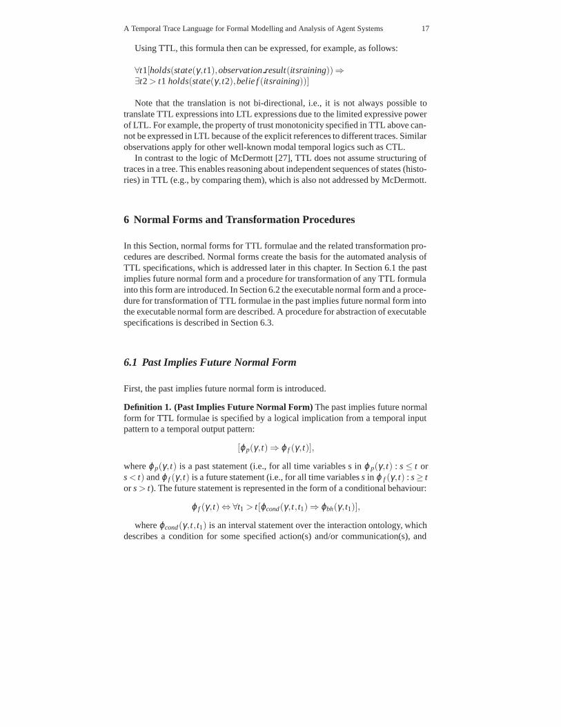
6.1 Past Implies Future Normal Form
First, the past implies future normal form is introduced.
Definition 1. (Past Implies Future Normal Form) The past implies future normalform for TTL formulae is specified by a logical implication from a temporal inputpattern to a temporal output pattern:
[ϕp(γ, t) ⇒ ϕ f (γ, t)],
where ϕ p(γ,t) is a past statement (i.e., for all time variables s in ϕ p(γ, t) : s ≤ t ors < t) and ϕ f (γ,t) is a future statement (i.e., for all time variables s in ϕ f (γ, t) : s ≥ tor s > t). The future statement is represented in the form of a conditional behaviour:
ϕ f (γ,t) ⇔∀t1 > t[ϕcond(γ, t, t1) ⇒ ϕbh(γ, t1)],
where ϕcond(γ,t,t1) is an interval statement over the interaction ontology, whichdescribes a condition for some specified action(s) and/or communication(s), and

18 Alexei Sharpanskykh and Jan Treur
Fig. 3 Graphical illustration of the structure of the past implies future normal form
ϕbh(γ,t1) is a (conjunction of) future statement(s) for t1 over the output ontology ofthe form holds(state(γ,t1 + c),out put(a)), for some integer constant c and actionor communication a.
A graphical illustration of the structure of the past implies future normal form isgiven in Figure 3. When a past formula ϕ p(γ, t) is true for γ at time t, a potentialto perform one or more action(s) and/or communication(s) exists. This potential isrealized at time t1 when the condition formula ϕ cond(γ, t, t1) becomes true, whichleads to the action(s) and/or communication(s) being performed at the time point(s)t1 + c indicated in ϕbh(γ,t1).
For example, the dynamic property DP7(A1,A2) (Information provision reac-tiveness) from the specification of co-operative information gathering multi-agentsystem from Section 4.1 can be specified in the past implies future normal formϕp(γ,t) ⇒ ϕ f (γ,t), with ϕp(γ, t) is a formula
∃t2 ≤ t & holds(state(γ,t2, input(A2)),communicated f rom to(A1,A2,request, IC))and ϕ f (γ,t) is a formula
∀t1 > t [holds(state(γ,t1, input(A2)),observation result to f or(A2, IC)) ⇒holds(state(γ,t1+ c,out put(A2)),communicated fromto(A2,A1, in f orm, IC))]
with ϕcond(γ,t,t1) is a formulaholds(state(γ,t1, input(A2)),observation result to f or(A2, IC))
and ϕbh(γ,t1) is holds(state(γ,t1+c,out put(A2)),communicated f rom to(A2,A1,in f orm, IC))],
where t is the present time point with respect to which the formulae are evaluatedand c is some natural number.
In general, any TTL formula can be automatically translated into the past im-plies future normal form. The transformation procedure is based on a number ofsteps. First, the variables in the formula are related to the given t (current timepoint) by differentiation. The resulting formula is rewritten in prenex conjunctivenormal form. Each clause in this formula is reorganised in past implies future for-mat. Finally, the quantifiers are distributed over and within these implications. Nowconsider the detailed description of these steps (for a more profound description ofthe procedure see [37]).
Differentiating Time Variables A formula is rewritten into an equivalent onesuch that time variables that occur in this formula always either are limited (rela-

A Temporal Trace Language for Formal Modelling and Analysis of Agent Systems 19
tivized) to past or to future time points with respect to t. As an example, supposeψ(t1,t2) is a formula in which time variables t1, t2 occur. Then, different cases of or-dering relation for each of the time variables with respect to t are considered: t 1 < t,t1 ≥ t and t2 < t, t2 ≥ t, i.e., in combination four cases: t1 < t and t2 < t, t1 < tand t2 ≥ t, t1 ≥ t and t2 < t, t1 ≥ t and t2 ≥ t. To eliminate ambiguity, for ti < t thevariable ti is replaced by (past time variable) ui, for ti ≥ t by (future time variable)vi.
The following transformation step introduces for any occurring time variable t i
a differentiation into a pair of new time variables: ui used over the past and vi usedover the future with respect to t.
For any occurrence of a universal quantifier over t i:∀ti A �−→ [∀ui < t A[ui/ti]∧∀vi ≥ t A[vi/ti]]For any occurrence of an existential quantifier over t i:∃ti A �−→ [∃ui < t A[ui/ti]∨∃vi ≥ t A[vi/ti]]Assuming differentiation of time variables into past and future time variables,
state-related atoms (in which only one time variable occurs) can be classified ina straightforward manner as a past atom or future atom. For example, atoms ofthe form holds(state(γ,ui), p) are past atoms and holds(state(γ,v j), p) are futureatoms. For non-unary relations, in the special case of the time ordering relation ¡ theordering axioms are given, e.g., transitivity. Atoms that are mixed (containing botha past and a future variable) are eliminated by the following transformation rules:
ui = v j → f alse v j < ui → f alse ui < v j → trueObtaining prenex conjunctive normal form This step is performed using a
well-known transformation procedure [15].From a Clause to a Past to Future Implication By partitioning the set of oc-
curring atoms into past atoms and future atoms, it is not difficult to rewrite a clauseinto a past to future implication format: transform a clause C into an implication ofthe form A → B where A is the conjunction of the negations of all past literals inC and B is the disjunction of all future literals in C. Thus, a quantifier free formulain Conjunctive Normal Form can be transformed into a conjunction of implicationsfrom past to future by the transformation rule
∨ PLi ∨ ∨FL j �−→ ∧ ∼ PLi →∨ FL j
where the past and future literals are indicated by PLi and FL j, respectively, andif a is an atom, ∼ a = ¬a, and ∼ ¬a = a.
Distribution of Quantifiers Over Implications The quantifiers can be rewrittento quantifiers with a single implication as their scope, and even one step further, toquantifiers with a single antecedent or a single consequent of an implication as theirscope. Notice that quantifiers addressed here are both time quantifiers and non-timequantifiers.
Let ϕ be a formula in the form of a conjunction of past to future implications∧i∈I [Ai → Bi] and let x be a (either past or future) variable occurring in ϕ . Thefollowing transformation rules handle existential quantifiers for variables in one ormore of the Bi, respectively in one or more of the Ai. Here P denotes taking thepower set.

20 Alexei Sharpanskykh and Jan Treur
1. if x occurs in the Bi but does not occur in the Ai :∃x ∧i∈I [Ai → Bi] �−→ ∧ j∈P(I) ∃x[∧i∈ jAi →∧i∈ jBi]∃x[∧i∈ jAi →∧i∈ jBi] �−→ [∧i∈ jAi →∃x∧i∈ j Bi]
2. if x occurs in the Ai but does not occur in the Bi :∃x∧i∈I [Ai → Bi] �−→ ∧ j∈P(I)∃x[∨i∈ jAi →∨i∈ jBi]∃x[∨i∈ jAi →∨i∈ jBi] �−→ [∀x[∨i∈ jAi] →∨i∈ jBi]
The following transformation rules handle universal quantifiers for variables inone or more of the Bi, respectively in one or more of the Ai:
1. if x occurs in the Ai or in the Bi :∀x ∧i∈I [Ai → Bi] �−→ ∧i∈I∀x[Ai → Bi]
2. if x occurs in the Bi but does not occur in the Ai :∀x[Ai → Bi] �−→ Ai →∀xBi
3. if x occurs in the Ai but does not occur in the Bi :∀x[Ai → Bi] �−→ [∃xAi] → Bi
6.2 Executable Normal Form
Although the past implies future normal form imposes a standard structure on therepresentation of TTL formulae, it does not guarantee the executability of formu-lae, required for automated analysis methods (i.e., some formulae may still containcomplex temporal relations that cannot be directly represented in analysis tools).Therefore, to enable automated analysis, normalized TTL formulae should be trans-lated into an executable normal form.
Definition 2. Executable Normal Form A TTL formula is in executable normalform if it has one of the following forms, for certain state properties , X and Y withX = Y , and integer constant c.
1. ∀t holds(state(γ,t),X) ⇒ holds(state(γ, t + c),Y ) (states relation property)2. ∀t holds(state(γ,t),X) ⇒ holds(state(γ, t + 1),X) (persistency property)3. ∀t holds(state(γ,t),X) ⇒ holds(state(γ, t),Y ) (state relation property)
For the translation postulated internal states of a component(s) specified in theformula, are used. These auxiliary states include memory states that are basedon (input) observations (sensory representations) or communications (memory :LTIMET ERMS ×STATPROP→ STATROP). For example, memory(t,observed(a))expresses that the component has memory that it observed a state property a attime point t. Furthermore, before performing an action or communication it ispostulated that a component creates an internal preparation state. For example,preparation f or(b) represents a preparation of a component to perform an actionor a communication.
In the following a transformation procedure from the normal form [ϕ p(γ, t) ⇒ϕ f (γ,t)] for the property ϕ p(γ, t) to the executable normal form is described and

A Temporal Trace Language for Formal Modelling and Analysis of Agent Systems 21
Fig. 4 A graphical representation of relations between interaction states described by a non-executable dynamic property and internal states described by executable rules.
illustrated for the property DP7(A1,A2) (Information provision reactiveness) con-sidered above. For a more profound description of the transformation procedure werefer to [35].
First, an intuitive explanation for the procedure is provided. The procedure trans-forms a non-executable dynamic property in a number of executable properties.These properties can be seen as an execution chain, which describes the dynam-ics of the non-executable property. In this chain each unit generates intermediatestates, used to link the following unit. In particular, first a number of propertiesare created to generate and maintain memory states (step 1 below). These memorystates are used to store information about the past dynamics of components, whichis available afterwards at any point in time. Then, executable properties are createdto generate preparation for output and output states of components (steps 2 and 3below). In these properties temporal patterns based on memory states are identifiedrequired for generation of particular outputs of components. In the end all createdproperties are combined in one executable specification.
More specifically, the transformation procedure consists of the following steps:
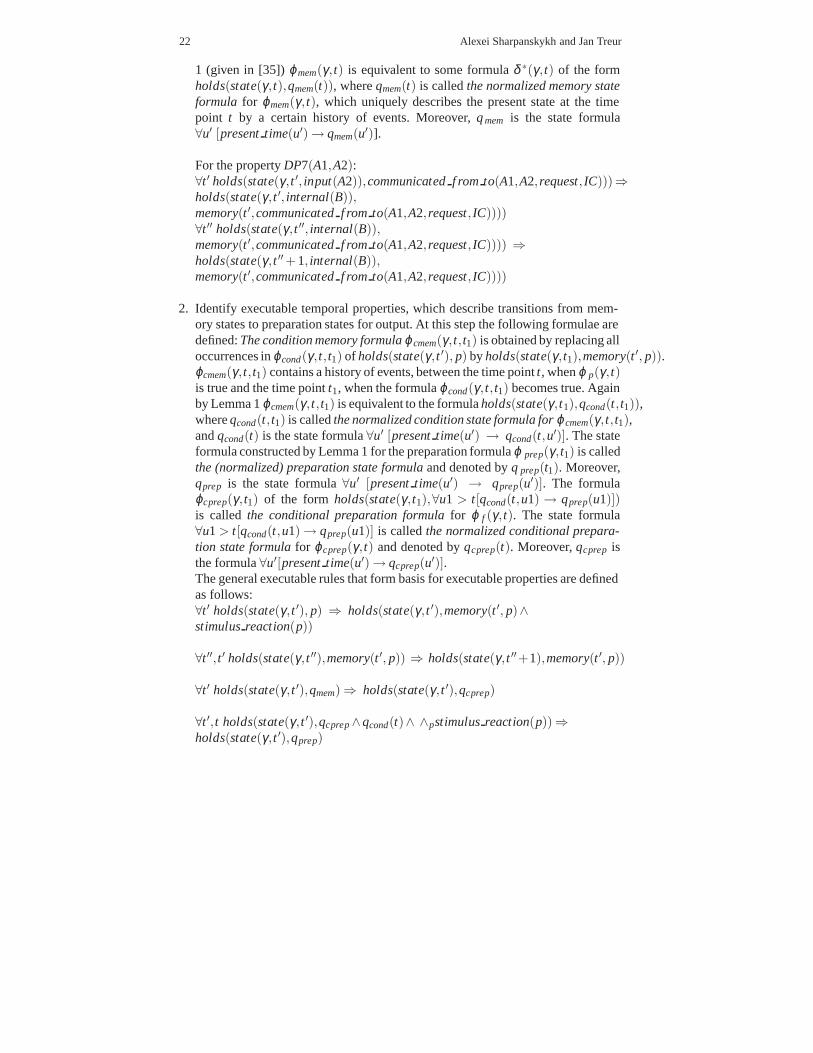
1. Identify executable temporal properties, which describe transitions from the com-ponent states specified in ϕ p(γ, t) to memory states (for a graphical representationof relations between the states considered in this procedure see Figure 4).The general rules that form the basis for the executable properties are the follow-ing:∀t ′ holds(state(γ,t ′), p) ⇒ holds(state(γ, t ′),memory(t ′, p))∀t ′′ holds(state(γ,t ′′),memory(t ′, p)) ⇒ holds(state(γ, t ′′ + 1),memory(t ′, p))
Furthermore, at this step the memory formula ϕ mem(γ, t) is defined that is ob-tained by replacing all occurrences in ϕ p(γ, t) of subformulae of the formholds(state(γ,t ′), p) by holds(state(γ, t),memory(t ′, p)). According to Lemma
22 Alexei Sharpanskykh and Jan Treur
1 (given in [35]) ϕmem(γ,t) is equivalent to some formula δ ∗(γ, t) of the formholds(state(γ,t),qmem(t)), where qmem(t) is called the normalized memory stateformula for ϕmem(γ,t), which uniquely describes the present state at the timepoint t by a certain history of events. Moreover, q mem is the state formula∀u′ [present time(u′) → qmem(u′)].
For the property DP7(A1,A2):∀t ′ holds(state(γ,t ′, input(A2)),communicated f rom to(A1,A2,request, IC)))⇒holds(state(γ,t ′, internal(B)),memory(t ′,communicated f rom to(A1,A2,request, IC))))∀t ′′ holds(state(γ,t ′′, internal(B)),memory(t ′,communicated f rom to(A1,A2,request, IC)))) ⇒holds(state(γ,t ′′+ 1, internal(B)),memory(t ′,communicated f rom to(A1,A2,request, IC))))
2. Identify executable temporal properties, which describe transitions from mem-ory states to preparation states for output. At this step the following formulae aredefined: The condition memory formula ϕ cmem(γ, t, t1) is obtained by replacing alloccurrences in ϕcond(γ,t,t1) of holds(state(γ, t ′), p) by holds(state(γ, t1),memory(t ′, p)).ϕcmem(γ,t,t1) contains a history of events, between the time point t, when ϕ p(γ, t)is true and the time point t1, when the formula ϕcond(γ, t, t1) becomes true. Againby Lemma 1 ϕcmem(γ,t,t1) is equivalent to the formula holds(state(γ, t1),qcond(t, t1)),where qcond(t,t1) is called the normalized condition state formula for ϕ cmem(γ, t, t1),and qcond(t) is the state formula ∀u′ [present time(u′) → qcond(t,u′)]. The stateformula constructed by Lemma 1 for the preparation formula ϕ prep(γ, t1) is calledthe (normalized) preparation state formula and denoted by q prep(t1). Moreover,qprep is the state formula ∀u′ [present time(u′) → qprep(u′)]. The formulaϕcprep(γ,t1) of the form holds(state(γ, t1),∀u1 > t[qcond(t,u1) → qprep(u1)])is called the conditional preparation formula for ϕ f (γ, t). The state formula∀u1 > t[qcond(t,u1) → qprep(u1)] is called the normalized conditional prepara-tion state formula for ϕcprep(γ, t) and denoted by qcprep(t). Moreover, qcprep isthe formula ∀u′[present time(u′) → qcprep(u′)].The general executable rules that form basis for executable properties are definedas follows:∀t ′ holds(state(γ,t ′), p) ⇒ holds(state(γ, t ′),memory(t ′, p)∧stimulus reaction(p))
∀t ′′,t ′ holds(state(γ,t ′′),memory(t ′, p)) ⇒ holds(state(γ, t ′′+1),memory(t ′, p))
∀t ′ holds(state(γ,t ′),qmem) ⇒ holds(state(γ, t ′),qcprep)
∀t ′,t holds(state(γ,t ′),qcprep ∧qcond(t)∧ ∧pstimulus reaction(p))⇒holds(state(γ,t ′),qprep)
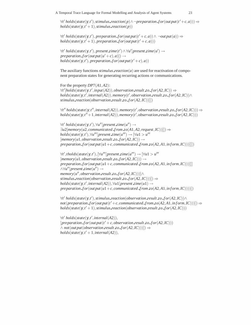
A Temporal Trace Language for Formal Modelling and Analysis of Agent Systems 23
∀t ′ holds(state(γ,t ′),stimulus reaction(p)∧¬preparation f or(out put(t ′+c,a)))⇒holds(state(γ,t ′+ 1),stimulus reaction(p))
∀t ′ holds(state(γ,t ′), preparation f or(out put(t ′+ c,a))∧ ¬out put(a))⇒holds(state(γ,t ′+ 1), preparation f or(out put(t ′+ c,a)))
∀t ′ holds(state(γ,t ′), present time(t ′)∧∀u′[present time(u′) →preparation f or(out put(u′+ c),a)]) →holds(state(γ,t ′), preparation f or(out put(t ′+ c),a))
The auxiliary functions stimulus reaction(a) are used for reactivation of compo-nent preparation states for generating recurring actions or communications.
For the property DP7(A1,A2):∀t ′[holds(state(γ,t ′, input(A2)),observation result to f or(A2, IC)) ⇒holds(state(γ,t ′, internal(A2)),memory(t ′,observation result to f or(A2, IC))∧stimulus reaction(observation result to f or(A2, IC))]])
∀t ′′ holds(state(γ,t ′′, internal(A2)),memory(t ′,observation result to f or(A2, IC)))⇒holds(state(γ,t ′′+1, internal(A2)),memory(t ′,observation result to f or(A2, IC)))
∀t ′ holds(state(γ,t ′),∀u′′[present time(u′′) →∃u2[memory(u2,communicated f rom to(A1,A2,request, IC))]])⇒holds(state(γ,t ′),∀u′′′[present time(u′′′) → [∀u1 > u′′′[memory(u1,observation result to f or(A2, IC)) →preparation f or(out put(u1+c,communicated f rom to(A2,A1, in f orm, IC)))]]])
∀t ′,tholds(state(γ,t ′), [∀u′′′[present time(u′′′) → [∀u1 > u′′′[memory(u1,observation result to f or(A2, IC))) →preparation f or(out put(u1+c,communicated f rom to(A2,A1, in f orm, IC)))]]]∧∀u′′[present time(u′′) →memory(u′′,observation result to f or(A2, IC)))]∧stimulus reaction(observation result to f or(A2, IC)))]) ⇒holds(state(γ,t ′, internal(A2)),∀u1[present time(u1) →preparation f or(out put(u1+c,communicated f rom to(A2,A1, in f orm, IC))))])
∀t ′ holds(state(γ,t ′),stimulus reaction(observation result to f or(A2, IC))∧not(preparation f or(out put(t ′+c,communicated f rom to(A2,A1, in f orm, IC)))])⇒holds(state(γ,t ′+ 1),stimulus reaction(observation result to f or(A2, IC)))
∀t ′ holds(state(γ,t ′, internal(A2)),[preparation f or(out put(t ′+ c,observation result to f or(A2, IC)))∧ not(out put(observation result to f or(A2, IC)))]) ⇒holds(state(γ,t ′+ 1, internal(A2)),

24 Alexei Sharpanskykh and Jan Treur
preparation f or(out put(t ′+ c,observation result to f or(A2, IC))))
3. Specify executable properties, which describe the transition from preparationstates to the corresponding output states.
The preparation state preparation f or(out put(t1+c,a)) is followed by the out-put state, created at the time point t1+c. The general executable rule is the follow-ing:∀t ′ holds(state(γ,t ′), preparation f or(out put(t ′+c,a))) ⇒ holds(state(γ, t ′+c),out put(a))
For the property DP7(A1,A2):∀t ′ holds(state(γ,t ′, internal(A2)),preparation f or(out put(t ′+c,communicated f rom to(A2,A1, in f orm, IC))))⇒holds(state(γ,t ′+ c,out put(A2)),out put(communicated f rom to(A2,A1, in f orm, IC)))
To automate the proposed procedure the software tool was developed in Java TM .The transformation algorithm searches in the input file for the standard predicatenames and the predefined structures, then performs string transformations that cor-respond precisely to the described steps of the translation procedure, and adds exe-cutable rules to the output specification file.
6.3 Abstraction of executable specifications
Sometimes (executable) specifications of multi-agent systems may be very detailed,with opaque global dynamics. To establish higher level dynamic properties of suchsystems, abstraction of specifications can be performed. In particular, internal dy-namics of agents described by executable cognitive specifications may be abstractedto behavioural (or interaction) specifications of agents as shown in [36]. To expressproperties of behavioural and cognitive specifications past and past-present state-ments are used.
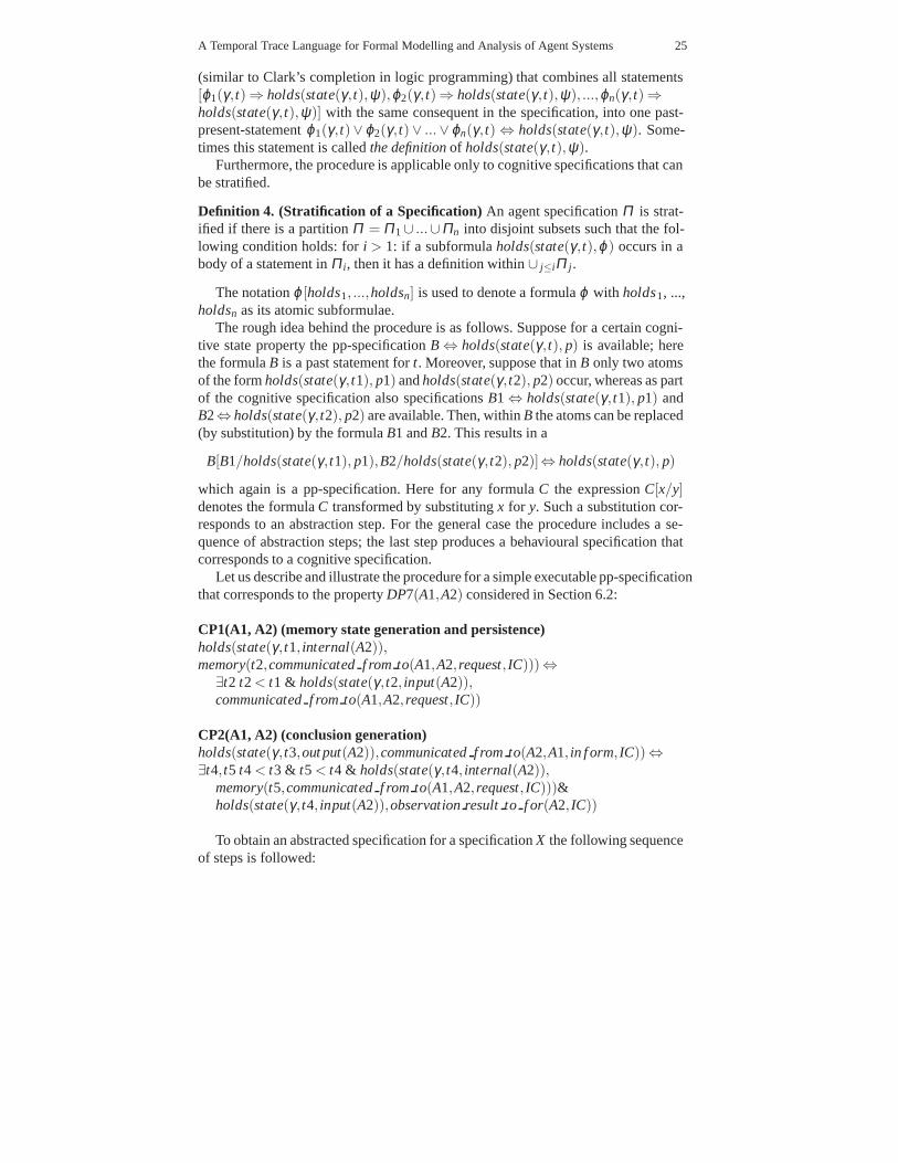
Definition 3. (Past-Present Statement) A past-present statement (abbreviated as app-statement) is a statement ϕ of the form B ⇔ H, where the formula B, called thebody and denoted by body(ϕ ), is a past statement for t, and H, called the head anddenoted by head(ϕ ), is a statement of the form holds(state(γ, t), p) for some stateproperty p.
It is assumed that each output state of an agent A specified by an atomholds(state(γ,t),ψ) is generated based on some input and internal agents dynamicsthat can be specified by a set of formulae over ϕ (γ, t)⇒ holds(state(γ, t),ψ) with ϕa past statement over InOnt(A)∪IntOnt(A). Furthermore, a completion can be made
A Temporal Trace Language for Formal Modelling and Analysis of Agent Systems 25
(similar to Clark’s completion in logic programming) that combines all statements[ϕ1(γ,t) ⇒ holds(state(γ,t),ψ),ϕ2(γ, t) ⇒ holds(state(γ, t),ψ), ...,ϕn(γ, t) ⇒holds(state(γ,t),ψ)] with the same consequent in the specification, into one past-present-statement ϕ1(γ,t)∨ ϕ2(γ, t)∨ ...∨ ϕn(γ, t) ⇔ holds(state(γ, t),ψ). Some-times this statement is called the definition of holds(state(γ, t),ψ).
Furthermore, the procedure is applicable only to cognitive specifications that canbe stratified.
Definition 4. (Stratification of a Specification) An agent specification Π is strat-ified if there is a partition Π = Π1 ∪ ...∪Πn into disjoint subsets such that the fol-lowing condition holds: for i > 1: if a subformula holds(state(γ, t),ϕ ) occurs in abody of a statement in Π i, then it has a definition within ∪ j≤iΠ j.
The notation ϕ [holds1, ...,holdsn] is used to denote a formula ϕ with holds1, ...,holdsn as its atomic subformulae.
The rough idea behind the procedure is as follows. Suppose for a certain cogni-tive state property the pp-specification B ⇔ holds(state(γ, t), p) is available; herethe formula B is a past statement for t. Moreover, suppose that in B only two atomsof the form holds(state(γ,t1), p1) and holds(state(γ, t2), p2) occur, whereas as partof the cognitive specification also specifications B1 ⇔ holds(state(γ, t1), p1) andB2⇔ holds(state(γ,t2), p2) are available. Then, within B the atoms can be replaced(by substitution) by the formula B1 and B2. This results in a
B[B1/holds(state(γ,t1), p1),B2/holds(state(γ, t2), p2)]⇔ holds(state(γ, t), p)
which again is a pp-specification. Here for any formula C the expression C[x/y]denotes the formula C transformed by substituting x for y. Such a substitution cor-responds to an abstraction step. For the general case the procedure includes a se-quence of abstraction steps; the last step produces a behavioural specification thatcorresponds to a cognitive specification.
Let us describe and illustrate the procedure for a simple executable pp-specificationthat corresponds to the property DP7(A1,A2) considered in Section 6.2:
CP1(A1, A2) (memory state generation and persistence)holds(state(γ,t1, internal(A2)),memory(t2,communicated f rom to(A1,A2,request, IC)))⇔
∃t2 t2 < t1 & holds(state(γ, t2, input(A2)),communicated f rom to(A1,A2,request, IC))
CP2(A1, A2) (conclusion generation)holds(state(γ,t3,out put(A2)),communicated f rom to(A2,A1, in f orm, IC))⇔∃t4,t5 t4 < t3 & t5 < t4 & holds(state(γ, t4, internal(A2)),
memory(t5,communicated f rom to(A1,A2,request, IC)))&holds(state(γ,t4, input(A2)),observation result to f or(A2, IC))
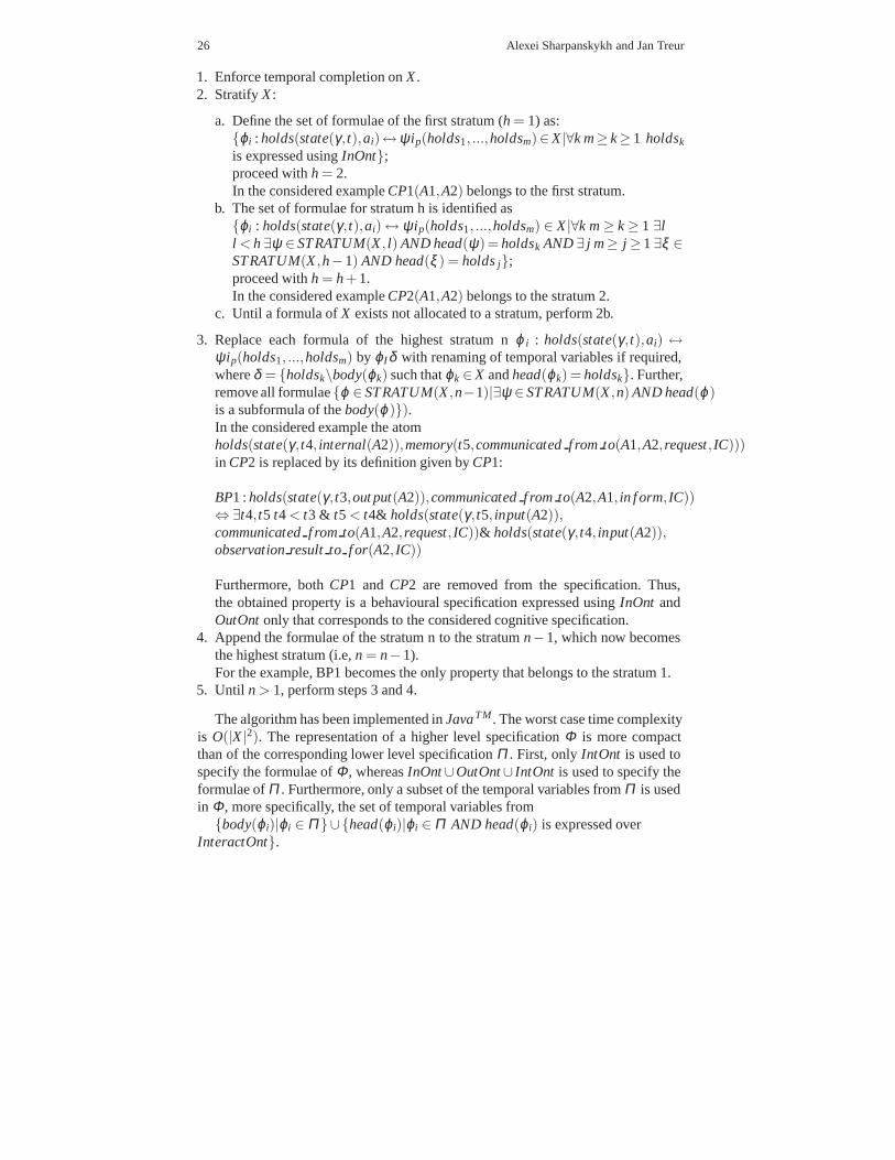
To obtain an abstracted specification for a specification X the following sequenceof steps is followed:
26 Alexei Sharpanskykh and Jan Treur
1. Enforce temporal completion on X .2. Stratify X :
a. Define the set of formulae of the first stratum (h = 1) as:{ϕi : holds(state(γ,t),ai)↔ψip(holds1, ...,holdsm)∈X |∀k m≥ k≥ 1 holdsk
is expressed using InOnt};proceed with h = 2.In the considered example CP1(A1,A2) belongs to the first stratum.
b. The set of formulae for stratum h is identified as{ϕi : holds(state(γ,t),ai) ↔ ψip(holds1, ...,holdsm) ∈ X |∀k m ≥ k ≥ 1 ∃ll < h ∃ψ ∈ STRATUM(X , l) AND head(ψ)= holdsk AND ∃ j m≥ j ≥ 1 ∃ξ ∈STRATUM(X ,h−1) AND head(ξ ) = holds j};proceed with h = h+ 1.In the considered example CP2(A1,A2) belongs to the stratum 2.
c. Until a formula of X exists not allocated to a stratum, perform 2b.
3. Replace each formula of the highest stratum n ϕ i : holds(state(γ, t),ai) ↔ψip(holds1, ...,holdsm) by ϕIδ with renaming of temporal variables if required,where δ = {holdsk\body(ϕk) such that ϕk ∈X and head(ϕk) = holdsk}. Further,remove all formulae {ϕ ∈ STRATUM(X ,n−1)|∃ψ ∈ STRATUM(X ,n) AND head(ϕ )is a subformula of the body(ϕ )}).In the considered example the atomholds(state(γ,t4, internal(A2)),memory(t5,communicated f rom to(A1,A2,request, IC)))in CP2 is replaced by its definition given by CP1:
BP1 : holds(state(γ,t3,out put(A2)),communicated f rom to(A2,A1, in f orm, IC))⇔∃t4,t5 t4 < t3 & t5 < t4& holds(state(γ, t5, input(A2)),communicated f rom to(A1,A2,request, IC))& holds(state(γ, t4, input(A2)),observation result to f or(A2, IC))
Furthermore, both CP1 and CP2 are removed from the specification. Thus,the obtained property is a behavioural specification expressed using InOnt andOutOnt only that corresponds to the considered cognitive specification.
4. Append the formulae of the stratum n to the stratum n−1, which now becomesthe highest stratum (i.e, n = n−1).For the example, BP1 becomes the only property that belongs to the stratum 1.
5. Until n > 1, perform steps 3 and 4.
The algorithm has been implemented in JavaTM . The worst case time complexityis O(|X |2). The representation of a higher level specification Φ is more compactthan of the corresponding lower level specification Π . First, only IntOnt is used tospecify the formulae of Φ, whereas InOnt ∪OutOnt ∪ IntOnt is used to specify theformulae of Π . Furthermore, only a subset of the temporal variables from Π is usedin Φ, more specifically, the set of temporal variables from
{body(ϕi)|ϕi ∈ Π }∪{head(ϕi)|ϕi ∈ Π AND head(ϕi) is expressed overInteractOnt}.

A Temporal Trace Language for Formal Modelling and Analysis of Agent Systems 27
7 Verification of Specifications of Multi-Agent Systems in TTL
In this Section two verification techniques of specifications of multi-agent systemsare considered. In Section 7.1 a verification approach of TTL specifications bymodel checking is discussed. Checking of TTL properties on a limited set of tracesobtained empirically or by simulation is considered in Section 7.2.
7.1 Verification of interlevel relations in TTL specifications bymodel checking
The dynamic properties of a component of a higher aggregation level can be log-ically related by an interlevel relation to dynamic properties of components of anadjacent lower aggregation level. This interlevel relation takes the form that a num-ber of properties of the lower level logically entail the properties of the higher levelcomponent.
Identifying interlevel relations is usually achieved by applying informal or semi-formal early requirements engineering techniques; e.g., i ∗ [11] and SADT [25].To formally prove that the identified interlevel relations are indeed correct, modelchecking techniques [10, 28] may be of use. The idea is that the lower level prop-erties in an interlevel relation are used as a system specification, whereas the higherlevel properties are checked for this system specification. However, model check-ing techniques are only suitable for systems specified as finite-state concurrent sys-tems. To apply model checking techniques it is needed to transform an original be-havioural specification of the lower aggregation level into a model based on a finitestate transition system. To obtain this, as a first step a behavioural description forthe lower aggregation level is replaced by one in executable temporal format usingthe procedure described in Section 6.2. After that, using an automated procedure anexecutable temporal specification is translated into a general finite state transitionsystem format that consists of standard transition rules. Such a representation canbe easily translated into an input format of one of the existing model checkers. Totranslate an executable specification into the finite state transition system format, foreach rule from the executable specification the corresponding transition rule shouldbe created. For translation the atom present time is used, which is evaluated to trueonly in a state for the current time point. For example, consider the translation ofthe memory state creation and persistence rules given in Table 3. The translation ofother rules is provided in [35].
The executable properties obtained in Section 6.2 for the property DP7(A1,A2)from the running example were translated into the transition rules as follows:
present time(t)∧ communicated f rom to(A,B,request, IC)−→memory(t,communicated f rom to(A,B,request, IC))
present time(t)∧observation result to f or(B, IC) −→

28 Alexei Sharpanskykh and Jan Treur
Table 3 Translation of the memory state creation and persistence rules into the correspondingfinite state transition rules
Rule from the executable specification Corresponding transition rules
Memory state creation rule∀t ′ holds(state(γ, t′), p) ⇒holds(state(γ, t′),memory(t′, p)) present time(t)∧ p −→ memory(t, p)Memory persistence rule∀t ′′holds(state(γ, t′′),memory(t′, p)) ⇒holds(state(γ, t′′ +1),memory(t′, p)) memory(t, p) −→ memory(t, p)
memory(t,observation result to f or(B, IC))∧stimulus reaction(observation result to f or(B, IC))
memory(t,communicated f rom to(A,B,request, IC)) −→memory(t,communicated f rom to(A,B,request, IC))
memory(t,observed(observation result to f or(B, IC)) −→memory(t,observed(observation result to f or(B, IC))
present time(t)∧∃u2 ≤ t memory(u2,communicated(request f rom to f or(A,B, IC))) −→conditional preparation f or(out put(communicated f rom to(B,A, in f orm, IC)))
present time(t)∧conditional preparation f or(out put(communicated f rom to(B,A, in f orm, IC)))∧memory(t,observed(observation result to f or(B, IC)))∧stimulus reaction(observed(observation result to f or(B, IC))) −→preparation f or(out put(t + c,communicated f rom to(B,A, in f orm, IC)))
present time(t)∧stimulus reaction(observed(observation result to f or(B, IC)))∧not(preparation f or(out put(t +c,communicated f rom to(B,A, in f orm, IC))))−→stimulus reaction(observed(observation result to f or(B, IC)))
preparation f or(out put(t + c,communicated f rom to(B,A, in f orm, IC)))∧not(out put(communicated f rom to(B,A, in f orm, IC))) −→preparation f or(out put(t + c,communicated f rom to(B,A, in f orm, IC)))
preparation f or(out put(t + c,communicated f rom to(B,A, in f orm, IC)))∧present time(t + c−1)−→out put(communicated f rom to(B,A, in f orm, IC))
The obtained general representation for a finite state transition system was usedfurther as a model for the model checker SMV [28]. SMV was used to perform
A Temporal Trace Language for Formal Modelling and Analysis of Agent Systems 29
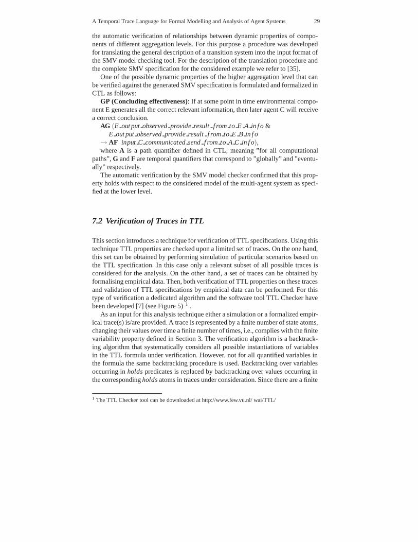
the automatic verification of relationships between dynamic properties of compo-nents of different aggregation levels. For this purpose a procedure was developedfor translating the general description of a transition system into the input format ofthe SMV model checking tool. For the description of the translation procedure andthe complete SMV specification for the considered example we refer to [35].
One of the possible dynamic properties of the higher aggregation level that canbe verified against the generated SMV specification is formulated and formalized inCTL as follows:
GP (Concluding effectiveness): If at some point in time environmental compo-nent E generates all the correct relevant information, then later agent C will receivea correct conclusion.
AG (E out put observed provide result f rom to E A in f o &E out put observed provide result f rom to E B in f o
→ AF input C communicated send f rom to A C in f o),where A is a path quantifier defined in CTL, meaning ”for all computational
paths”, G and F are temporal quantifiers that correspond to ”globally” and ”eventu-ally” respectively.
The automatic verification by the SMV model checker confirmed that this prop-erty holds with respect to the considered model of the multi-agent system as speci-fied at the lower level.
7.2 Verification of Traces in TTL
This section introduces a technique for verification of TTL specifications. Using thistechnique TTL properties are checked upon a limited set of traces. On the one hand,this set can be obtained by performing simulation of particular scenarios based onthe TTL specification. In this case only a relevant subset of all possible traces isconsidered for the analysis. On the other hand, a set of traces can be obtained byformalising empirical data. Then, both verification of TTL properties on these tracesand validation of TTL specifications by empirical data can be performed. For thistype of verification a dedicated algorithm and the software tool TTL Checker havebeen developed [7] (see Figure 5) 1 .
As an input for this analysis technique either a simulation or a formalized empir-ical trace(s) is/are provided. A trace is represented by a finite number of state atoms,changing their values over time a finite number of times, i.e., complies with the finitevariability property defined in Section 3. The verification algorithm is a backtrack-ing algorithm that systematically considers all possible instantiations of variablesin the TTL formula under verification. However, not for all quantified variables inthe formula the same backtracking procedure is used. Backtracking over variablesoccurring in holds predicates is replaced by backtracking over values occurring inthe corresponding holds atoms in traces under consideration. Since there are a finite
1 The TTL Checker tool can be downloaded at http://www.few.vu.nl/ wai/TTL/
30 Alexei Sharpanskykh and Jan Treur
number of such state atoms in the traces, iterating over them often will be moreefficient than iterating over the whole range of the variables occurring in the holdsatoms.
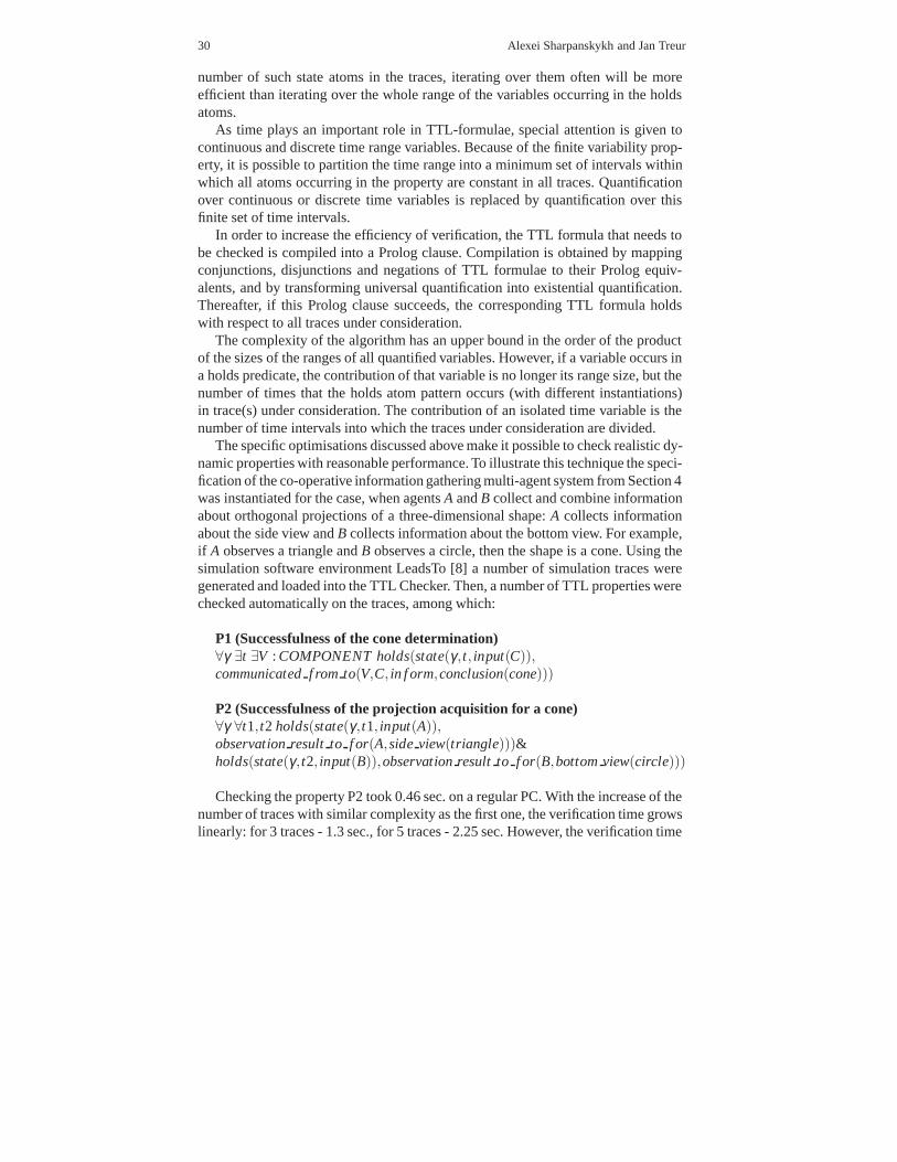
As time plays an important role in TTL-formulae, special attention is given tocontinuous and discrete time range variables. Because of the finite variability prop-erty, it is possible to partition the time range into a minimum set of intervals withinwhich all atoms occurring in the property are constant in all traces. Quantificationover continuous or discrete time variables is replaced by quantification over thisfinite set of time intervals.
In order to increase the efficiency of verification, the TTL formula that needs tobe checked is compiled into a Prolog clause. Compilation is obtained by mappingconjunctions, disjunctions and negations of TTL formulae to their Prolog equiv-alents, and by transforming universal quantification into existential quantification.Thereafter, if this Prolog clause succeeds, the corresponding TTL formula holdswith respect to all traces under consideration.
The complexity of the algorithm has an upper bound in the order of the productof the sizes of the ranges of all quantified variables. However, if a variable occurs ina holds predicate, the contribution of that variable is no longer its range size, but thenumber of times that the holds atom pattern occurs (with different instantiations)in trace(s) under consideration. The contribution of an isolated time variable is thenumber of time intervals into which the traces under consideration are divided.
The specific optimisations discussed above make it possible to check realistic dy-namic properties with reasonable performance. To illustrate this technique the speci-fication of the co-operative information gathering multi-agent system from Section 4was instantiated for the case, when agents A and B collect and combine informationabout orthogonal projections of a three-dimensional shape: A collects informationabout the side view and B collects information about the bottom view. For example,if A observes a triangle and B observes a circle, then the shape is a cone. Using thesimulation software environment LeadsTo [8] a number of simulation traces weregenerated and loaded into the TTL Checker. Then, a number of TTL properties werechecked automatically on the traces, among which:
P1 (Successfulness of the cone determination)∀γ ∃t ∃V : COMPONENT holds(state(γ, t, input(C)),communicated f rom to(V,C, in f orm,conclusion(cone)))
P2 (Successfulness of the projection acquisition for a cone)∀γ ∀t1,t2 holds(state(γ,t1, input(A)),observation result to f or(A,side view(triangle)))&holds(state(γ,t2, input(B)),observation result to f or(B,bottom view(circle)))
Checking the property P2 took 0.46 sec. on a regular PC. With the increase of thenumber of traces with similar complexity as the first one, the verification time growslinearly: for 3 traces - 1.3 sec., for 5 traces - 2.25 sec. However, the verification time
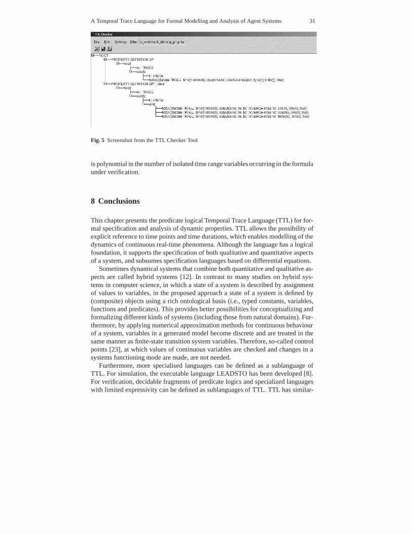
A Temporal Trace Language for Formal Modelling and Analysis of Agent Systems 31
Fig. 5 Screenshot from the TTL Checker Tool
is polynomial in the number of isolated time range variables occurring in the formulaunder verification.
8 Conclusions
This chapter presents the predicate logical Temporal Trace Language (TTL) for for-mal specification and analysis of dynamic properties. TTL allows the possibility ofexplicit reference to time points and time durations, which enables modelling of thedynamics of continuous real-time phenomena. Although the language has a logicalfoundation, it supports the specification of both qualitative and quantitative aspectsof a system, and subsumes specification languages based on differential equations.
Sometimes dynamical systems that combine both quantitative and qualitative as-pects are called hybrid systems [12]. In contrast to many studies on hybrid sys-tems in computer science, in which a state of a system is described by assignmentof values to variables, in the proposed approach a state of a system is defined by(composite) objects using a rich ontological basis (i.e., typed constants, variables,functions and predicates). This provides better possibilities for conceptualizing andformalizing different kinds of systems (including those from natural domains). Fur-thermore, by applying numerical approximation methods for continuous behaviourof a system, variables in a generated model become discrete and are treated in thesame manner as finite-state transition system variables. Therefore, so-called controlpoints [23], at which values of continuous variables are checked and changes in asystems functioning mode are made, are not needed.
Furthermore, more specialised languages can be defined as a sublanguage ofTTL. For simulation, the executable language LEADSTO has been developed [8].For verification, decidable fragments of predicate logics and specialized languageswith limited expressivity can be defined as sublanguages of TTL. TTL has similar-

32 Alexei Sharpanskykh and Jan Treur
ities (as well as important conceptual distinctions) with (from) situation and eventcalculi. A proper subclass of TTL formulae can be directly translated into formulaeof temporal logics (e.g., LTL and CTL).
In this chapter an automatically supported technique for verifying TTL proper-ties on a limited set of simulation or empirical traces was described. Furthermore,it was shown how model checking techniques can be used for verification of TTLspecifications. To enable model checking, a model should be provided in the form ofa finite state transition system. In this chapter it was shown how a TTL specificationthat comprises formulae in the executable normal form can be automatically trans-lated into a finite state transition system. Using such an approach relations betweendynamic properties of adjacent aggregation levels of a multi-agent system can bechecked automatically, as also demonstrated in this chapter. The proposed approachhas similarities with compositional reasoning and verification techniques [18] in theway how it handles complex dynamics of a system. Compositional reasoning ap-proaches developed in the area of software engineering are based on one commonidea that the analysis of global properties of a software system can be reduced to theanalysis of local properties of system components. More specifically, the problemof satisfaction of global properties of a complex software system can be reduced totwo (easier) problems: (i) identifying and justifying relations between global proper-ties of the system and local properties of its components (parts); (ii) verifying localproperties of system components with respect to components specifications.
In [30] formal methods for the analysis of hardware specifications expressed inthe language PSL (an extension of the standard temporal logics LTL and CTL), aredescribed. By means of the suggested property assurance technique supported by atool, different global system properties (e.g., consistency) can be verified on speci-fications and in such a way the correctness of specifications can be established. Theverification is based on bounded model checking techniques. Besides the specifi-cation language, an essential difference between this analysis method and the ap-proach described in this chapter is that the latter provides means for the multi-level(or compositional) representation and verification of properties in specifications.This allows system modelling at a necessary level of abstraction and the reductionof the complexity of verification of system dynamics.
Similar differences can be identified in comparison with the approach proposedin [16]. This approach allows semi-automatic formalization of informal graphicalspecifications of multi-agent systems with the subsequent verification of dynamicproperties using model checking techniques. Formalized specifications comprise de-scriptions of classes that describe components of a multi-agent system and relationsbetween them, constraints over these components, assertions and possibilities. Al-though the first-order temporal logic that is used for formalizing these specificationsis expressive enough to define complex temporal relations, it is does not provide thecomplete expressivity allowed by TTL (e.g., arithmetical operations, references tomultiple traces in the same formula). Furthermore, although such specifications canbe built and analyzed in parts, the idea of compositional verification, central in ourapproach, is not elaborated in this approach.
A Temporal Trace Language for Formal Modelling and Analysis of Agent Systems 33
Compositional verification may be used for analysis of dynamics of large socio-technical systems (e.g., in the area of incident management). Such systems are char-acterized by a large complexity of internal dynamics of and interaction among di-verse types of agents, including human and artificial intelligent agents (e.g., ambi-ent devices). It is expected that in the future the complexity of such systems willincrease considerably with a further development and implementation of ambientintelligence technologies. Formal analysis of such systems presents a big concep-tual and computational challenge for existing verification tools in the area of multi-agent systems. To enable effective and efficient analysis of systems of such type,new methods based on appropriate (dynamic) abstraction mechanisms need to bedeveloped. For this the idea of compositional verification may serve as the startingpoint. Further, findings from the area of nonlinear system analysis, control theoryand complex systems in general could be used.
Finally, TTL and the related analysis techniques proved their value in a numberof research projects in such disciplines as artificial intelligence, cognitive science,biology, and social science. In particular, the analysis of continuous models (i.e.,based on differential equations) is illustrated by the case study on trace conditioningconsidered in [9]. In [6] TTL is used for modelling and analysis of adaptive agentbehaviour specified by complex temporal relations. The use of arithmetical opera-tions in TTL to perform statistical analysis is illustrated by a case study from thecriminology [5]. More examples of applications of TTL are described in [7].
References
1. Ackermann, W.: Solvable Cases of the Decision Problem. North-Holland Publishing Com-pany, Amsterdam (1962)
2. Andreka, H., van Benthem, J., Nemeti, I.: Modal languages and bounded fragments of predi-cate logic. Journal of Philosophical Logic 27, 217–274 (1998)
3. Barringer, H., Fisher, M., Gabbay, D., Owens, R., Reynolds, M.: The Imperative Future: Prin-ciples of Executable Temporal Logic. John Wiley & Sons (1996)
4. van Benthem, J.: The Logic of Time: A Model-theoretic Investigation into the Varieties ofTemporal Ontology and Temporal Discourse. Reidel, Dordrecht (1983)
5. Bosse, T., Gerritsen, C., Treur, J.: Cognitive and social simulation of criminal behaviour: theintermittent explosive disorder case. In: Proceedings of the Sixth International Joint Con-ference on Autonomous Agents and Multi-Agent Systems, AAMAS’07, pp. 367–374. ACMPress (2007)
6. Bosse, T., Jonker, C., Los, S., van der Torre, L., Treur, J.: Formal analysis of trace conditioning.Cognitive Systems Research Journal 8, 36–47 (2007)
7. Bosse, T., Jonker, C., van der Meij, L., Sharpanskykh, A., Treur, J.: Specification and verifica-tion of dynamics in agent models. International Journal of Cooperative Information Systems18(1), 167–193 (2009)
8. Bosse, T., Jonker, C., van der Meij, L., Treur, J.: A language and environment for analysis ofdynamics by simulation. International Journal of Artificial Intelligence Tools 16(3), 435–464(2007)
9. Bosse, T., Sharpanskykh, A., Treur, J.: Modelling complex systems by integration of agent-based and dynamical systems models. In: A. Minai, D. Braha, Y. Bar-Yam (eds.) UnifyingThemes in Complex Systems VI, Proceedings of the Sixth International Conference on Com-plex Systems. Springer (2008)

34 Alexei Sharpanskykh and Jan Treur
10. Clarke, E., Grumberg, O., Peled, D.: Model Checking. MIT Press (2000)11. Cysneiros, L., Yu., E.: Requirements engineering for large-scale multi-agent systems. In:
Proceedings of the 1st International Central and Eastern European Conference on Multi-AgentSystems (CEEMAS’02), pp. 39–56. Springer Verlag (2002)
12. Davoren, J., Nerode, A.: Logics for hybrid systems. Proceedings of the IEEE 88(7), 985–1010(2000)
13. Dignum, V. (ed.): Multi-Agent Systems - Semantics and Dynamics of Organizational Models.IGI Global (2009)
14. Ferber, J., Gutknecht, O., Michel, F.: From Agents to Organizations: An Organizational Viewof Multi-agent Systems, vol. 2935, pp. 214–230. Springer (2004)
15. Fitting, M.: First-order Logic and Automated Theorem Proving. MIT Press, Springer Verlag(1996)
16. Fuxman, A., Liu, L., Pistore, M., Roveri, M., Mylopoulos, J.: Specifying and analyzing earlyrequirements in tropos. Requirements Engineering Journal 9(2), 132–150 (2004)
17. Goldblatt, R.: Logics of Time and Computation, CSLI Lecture Notes, vol. 7, 2nd edn. Springer(1992)
18. Hooman, J.: Compositional verification of a distributed real-time arbitration protocol. Real-Time Systems 6, 173–206 (1994)
19. Horling, B., Lesser, V.: A survey of multi-agent organizational paradigms. The KnowledgeEngineering Review 19(4), 281–316 (2004)
20. Jonker, C., Sharpanskykh, A., Treur, J., Yolum, P.: A framework for formal modeling andanalysis of organizations. Applied Intelligence 27(1), 49–66 (2007)
21. Jonker, C., Treur, J.: Compositional verification of multi-agent systems: a formal analysis ofpro-activeness and reactiveness. International Journal of Cooperative Information Systems 11,51–92 (2002)
22. Kowalski, R., Sergot, M.: A logic-based calculus of events. New Generation Computing 4,67–95 (2002)
23. Manna, Z., Pnueli, A.: Verifying Hybrid Systems, vol. 736, pp. 4–35. Springer (1993)24. Manzano, M.: Extensions of First Order Logic. Cambridge University Press (1996)25. Marca, D.: SADT: Structured Analysis and Design Techniques. McGraw-Hill, Cambridge
MA (1988)26. Mazurkiewicz, A.: Trace Theory, in Advances in Petri nets II: applications and relationships
to other models of concurrency, LNCS, vol. 255. Springer (1987)27. McDermott, D.: A temporal logic for reasoning about processes and plans. Cognitive Science
6, 101–155 (1982)28. McMillan, K.: Symbolic Model Checking. Kluwer Academic Publishers (1993)29. Pearson, C.: Numerical Methods in Engineering and Science. CRC Press (1986)30. Pill, I., Semprini, S., Cavada, R., Roveri, M., Bloem, R., Cimatti, A.: Formal analysis of hard-
ware requirements. In: Proceedings of the 43rd annual conference on Design automation(DAC ’06) (2006)
31. Pinto, J., Reiter, R.: Reasoning about time in the situation calculus. Ann. Math. Artif. Intell14, 251–268 (1995)
32. Port, R., van Gelder, T. (eds.): Mind as Motion: Explorations in the Dynamics of Cognition.MIT Press (1995)
33. Purdy, W.: Fluted formulas and the limits of decidability. Journal of Symbolic Logic 61,608–620 (1996)
34. Reiter, R.: Knowledge in Action: Logical Foundations for Specifying and Implementing Dy-namical Systems. MIT Press, Cambridge MA (2001)
35. Sharpanskykh, A., Treur, J.: Verifying interlevel relations within multi-agent systems. In:Proceedings of the 17th European Conference on Artificial Intelligence, ECAI’06, pp. 290–294. IOS Press (2006)
36. Sharpanskykh, A., Treur, J.: Relating cognitive process models to behavioural models ofagents. In: Proceedings of the 8th IEEE/WIC/ACM International Conference on IntelligentAgent Technology, IAT’08, pp. 330–335. IEEE Computer Society Press (2008)
A Temporal Trace Language for Formal Modelling and Analysis of Agent Systems 35
37. Treur, J.: Past-future separation and normal forms in temporal predicate logic specifi-cations. Journal of Algorithms in Cognition, Informatics and Logic 64 (2009). Doihttp://dx.doi.org/10.1016/j.jalgor.2009.02.008 (in press)